Disturbance Observer-Based Actor–Critic Reinforcement Learning with Adaptive Reward for Energy-Efficient Control of Robotic Manipulators

Abstract

Reinforcement learning controllers for robot manipulators depend strongly on reward tuning, and fixed weights may yield poor trade-offs under uncertainty and disturbances. This paper proposes a disturbance observer-based actor–critic RL (DOB–ACRL) with adaptive multi-objective reward shaping for a torque-saturated 2-DOF manipulator, where the reward weights are updated online using normalized indicators of tracking error, control energy, and effort. A Lyapunov analysis guarantees the uniform ultimate boundedness of closed-loop signals. The simulations show improved learning and performance over a static reward actor–critic baseline, reducing the RMS tracking error by up to 22.8%, the control energy by ~4.6%, the control effort by 1.9%, and the settling time by up to 29.2%.

1. Introduction

Robotic manipulators are increasingly being used in applications that demand accurate and robust tracking while also reducing energy consumption and ensuring long-term efficient operation [1,2,3,4,5]. Classical nonlinear and robust control, as well as disturbance observer (DOB) techniques, can effectively handle model uncertainties and external disturbances [6,7,8,9,10]. However, they are typically designed around a single (or fixed) performance index, making it challenging to tune when balancing the tracking accuracy, energy usage, and control effort simultaneously [11,12,13,14,15,16].

Reinforcement learning (RL), particularly actor–critic and adaptive dynamic programming (ADP), has therefore garnered attention for the optimal control of nonlinear systems with partially known dynamics [17,18,19,20,21,22,23,24,25,26,27,28]. Actor–critic structures approximate both the policy and the value function, enabling practical solutions to continuous-time, infinite-horizon problems, and have been applied to manipulators with stability and robustness enhancements (including Lyapunov arguments and, in some cases, DOB integration) [29,30,31,32]. However, most RL-based manipulator controllers still rely on a fixed, manually tuned scalar reward (typically a weighted sum of tracking, energy, and effort terms), which can lead to unstable learning and poor trade-offs when scaling changes or disturbances are significant [33,34,35,36,37]. As a result, explicit and systematic adaptive multi-objective reward design, especially when combined with DOBs, remains relatively limited [38,39,40].

Motivated by these research gaps, and building upon recent advancements in deep learning-based disturbance observation [41,42] and robust control for uncertain systems [43], this paper investigates a torque-saturated planar 2-DOF manipulator under uncertainty. We propose a disturbance observer-based actor–critic reinforcement learning (DOB–ACRL) framework with an adaptive multi-objective reward-shaping mechanism to optimally balance the tracking accuracy, energy consumption, and control effort. The primary contributions are as follows:

• Adaptive Reward Shaping: Unlike existing methods that rely on fixed gain adjustments [44], the reward function in this study is decomposed into tracking error, energy, and control effort components, with their weights updated online via normalized performance indicators.
• Lyapunov-based Stability Guarantee: Sufficient conditions are established to ensure the uniform ultimate boundedness (UUB) of all closed-loop signals. This analysis explicitly accounts for bounded disturbances, DOB estimation errors, and actor–critic approximation errors, extending the robustness frameworks discussed in the recent literature [45].
• Comparative Evaluation: The simulation results on a 2-DOF manipulator demonstrate superior performance in both the accuracy and efficiency compared to two baselines: a static reward actor–critic and an adaptive reward actor–critic without a DOB.

The remainder of the paper is organized as follows: Section 2 reviews the related work, Section 3 presents the system model and architecture, Section 4 details the adaptive reward and stability analysis, Section 5 reports the simulation results, Section 6 discusses the implications and limitations, and Section 7 concludes with future directions.

2. Related Work

The research related to this study can be grouped into three streams: (i) stability-guaranteed actor–critic and ADP control, (ii) reward shaping and adaptive and evolving rewards in RL, and (iii) DOB-based and energy-aware robotic control. The following review highlights the gaps motivating our approach [1,2,3].

2.1. Actor–Critic and ADP with Stability Guarantees

Actor–critic and ADP have been widely studied for optimal control of nonlinear systems with partially known dynamics, with continuous-time formulations and approximate solutions to infinite-horizon problems [4,5,6]. A large body of work has further developed stability and convergence guarantees using Lyapunov and Bellman error arguments, including robust/observer-based variants to handle uncertainties and disturbances [7,8,9]. These methods have also been applied to robotic systems and manipulators to achieve stable tracking and disturbance rejection under learning-based control structures [10,11,12]. Survey and overview papers have summarized the theoretical foundations and practical implementations of RL and ADP for control [13,14,15].

However, most stability-guaranteed actor–critic and ADP designs assume a fixed reward and cost (often a weighted sum of tracking and effort), and their analyses focus on the stability under that static index, with limited emphasis on the online adaptation of objective weights to handle multi-objective trade-offs [16,17,18].

2.2. Reward Shaping and Adaptive and Evolving Rewards

Reward shaping modifies the reward signal to accelerate learning or inject prior knowledge, with classic constructions that can preserve optimal policies under certain conditions [19,20,21]. Recent research has explored self-adaptive or evolving rewards that adjust the reward components online to improve the learning speed and empirical performance [22,23,24]. Related directions include shaping via stability and CLF-inspired terms or hybrid control and RL designs, where the reward is tuned implicitly to meet the performance constraints [25,26,27].

Despite these advances, much of the literature focuses on general MDP settings or benchmarks, and often fails to address continuous-time rigid-body manipulator dynamics, explicit DOB integration, or Lyapunov-style stability guarantees required in safety-critical robotic control [28,29,30].

2.3. Disturbance Observers, RL, and Energy-Efficient Manipulator Control

DOB-based control is a standard tool for compensating for lumped uncertainties and external disturbances in nonlinear systems and manipulators [31,32,33]. In parallel, energy-aware manipulator control has been studied through optimal and robust formulations that explicitly penalize the energy or actuator work, alongside broader perspectives on efficiency and sustainability [34,35,36]. Recent works have combined DOB and robust compensation with RL or ADP, leveraging a DOB to mitigate disturbances while RL and ADP optimize the performance under compensated dynamics [37,38,39].

Recent studies have increasingly explored the synergy between reinforcement learning (RL) and disturbance observers (DOBs) to handle uncertain nonlinear systems [40,41], with some works focusing on the stringent performance requirements in robotics [42,43]. For instance, Lee et al. [44] utilized deep RL for dynamic gain adjustment in DOBs, while Lee et al. [45] addressed the parametric uncertainties in UAV dynamics. Despite these advances, the existing DOB + RL approaches often rely on fixed reward structures and lack a unified framework that (i) adaptively schedules the objective weights online and (ii) ensures Lyapunov-based stability. This motivates our proposed DOB–ACRL framework, which incorporates an adaptive reward-shaping mechanism to dynamically balance the tracking accuracy and energy efficiency while maintaining rigorous boundedness guarantees.

3. System Model and Control Architecture

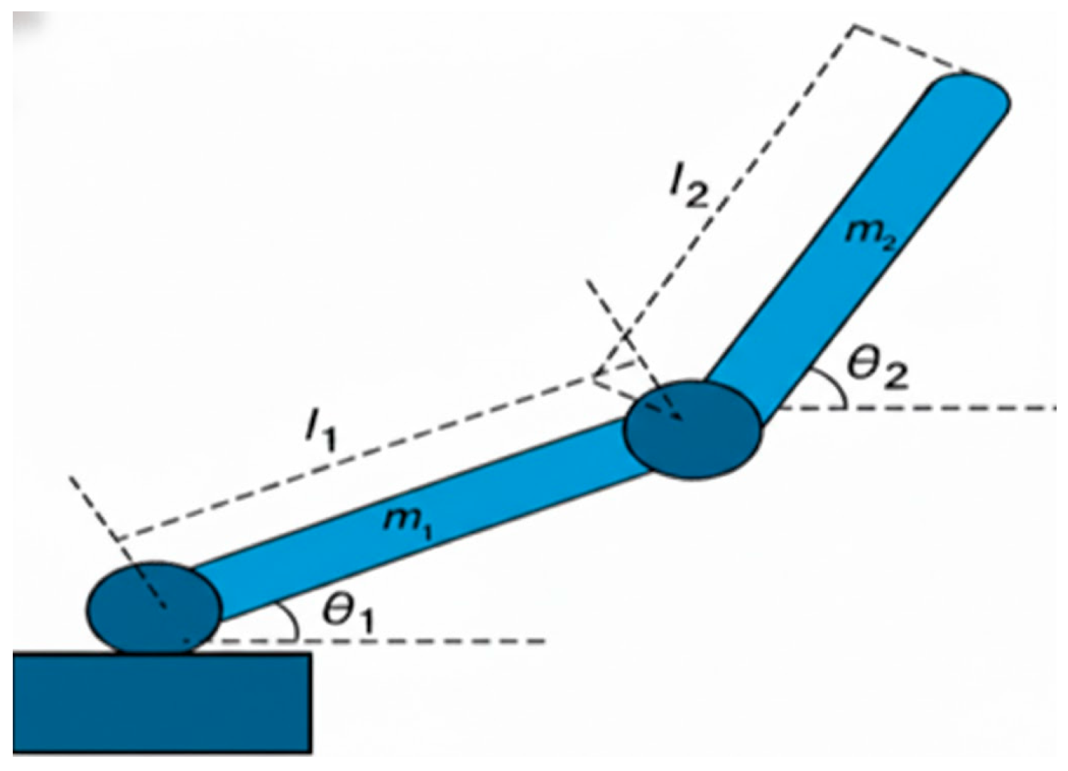
This section presents the 2-DOF manipulator model, illustrated in Figure 1, the tracking error dynamics used for control design, and the overall DOB–ACRL architecture.

We also define the multi-objective control goals (tracking accuracy, energy consumption, and torque smoothness) that will be combined through an adaptive reward-weighting scheme. The manipulator dynamics are given by

$$\mathit{M}(\mathit{q})\ddot{\mathit{q}}+\mathit{C}(\mathit{q},\dot{\mathit{q}})\dot{\mathit{q}}+\mathit{F}\dot{\mathit{q}}+\mathit{d}(t)=\mathit{\tau }$$

(1)

where $\mathit{M}(\mathit{q}),\mathit{C}(\mathit{q},\dot{\mathit{q}})$, and $\mathit{F}$ represent the inertia, Coriolis, and friction matrices, respectively; and $d\left(t\right)$ denotes the matched disturbances. Let $z_1=\mathit{q}-{\mathit{y}}_r,{ \mathrm{z}}_2=\dot{\mathit{q}}-{\dot{\mathit{y}}}_r+k_1{z}_1$ be the tracking and filtered errors. The actor–critic policy structure follows

$$\mathit{u}=\mathit{M}(\mathit{q})({\ddot{\mathit{y}}}_r-k_1{z}_1-k_2{z}_2-\widehat{\mathit{f}}(.)-\widehat{\mathit{d}}\left(t\right))$$

(2)

where $\widehat{\mathit{f}}(.)$ approximates the unmodeled dynamics and $\widehat{\mathit{d}}\left(t\right)$ is the DOB-estimated disturbance.

The adaptive composite reward is defined as

$${\mathit{r}}_t={\mathit{w}}_t(-z_1^{\top }\mathit{Q}{z}_1)+{\mathit{w}}_e(-\Vert \mathit{u}{\Vert }_2^2)+{\mathit{w}}_c(-\Vert \mathit{u}{\Vert }_1)$$

(3)

subject to $w_t+w_e+w_c=1, w_i>0$. Let $i\in \{t,e,c\}$, where $w_t$ is the tracking accuracy weight, $w_e$ is the energy efficiency weight, and $w_c$ is the control effort smoothness weight. The weighting coefficients are adapted online as

$$w_i(t)={\displaystyle \frac{e^{-{\beta }_i{\varphi }_i(t)}}{{\displaystyle \sum _j{e}^{-{\beta }_j{\varphi }_j(t)}}}}$$

(4)

where ${\varphi }_i\left(t\right)$ corresponds to the normalized performance indices, RMS tracking error, control energy, and control effort, respectively; and ${\beta }_i$ is the adaptation gains. The weights are updated online using normalized indicators, as detailed by Equations (8) and (9) in Section 4.1, where Equation (8) defines the exponential preference scores (from the normalized performance indicators) and Equation (9) specifies the smoothing/normalization update rule for the weights. As the RMS tracking error decreases, the policy automatically shifts emphasis toward minimizing the energy and control effort, emulating human-like “attention reallocation” during learning [23,40].

The disturbances and modeling uncertainties are the factors that significantly impact system performance and robustness. Furthermore, a detailed framework for quantifying and mitigating these effects is presented to validate the resilience and accuracy of the proposed control or estimation strategy. The disturbance $\mathit{d}(t)$ aggregates the external forces, unmodeled dynamics, and parameter uncertainties. We adopt the following standard assumptions:

Assumption 1

(bounded disturbance). The disturbance vector $\mathit{d}(t)$ is bounded for all $t\ge 0$, i.e., there exists a known constant ${\mathit{d}}_{\max }>0$, such that $|\mathit{d}(t)|\le d_{\max },\hspace{1em}\forall t\ge 0$.

Assumption 2

(bounded parameter uncertainty). The manipulator parameters used in the nominal model $\mathit{M}(q),\mathit{C}(q,\dot{q}),\mathit{F}(\dot{q})$ may differ from the true physical parameters, but the resulting model mismatch is bounded and can be lumped into the disturbance term d(t).

These assumptions are common in disturbance observer-based and robust nonlinear control, and allow us to treat all the unmodeled dynamics and uncertainties within a unified disturbance framework.

Disturbance Observer and Estimation Error

To mitigate the effect of $\mathit{d}(t)$, a disturbance observer (DOB) is employed. Based on the nominal model and measured signals $\mathit{q},\dot{\mathit{q}}$, the DOB generates an estimate $\widehat{\mathit{d}}(t)$ of the disturbance. The corresponding estimation error is defined as

$$\tilde{\mathit{d}}(t)=\mathit{d}(t)-\widehat{\mathit{d}}(t)$$

(5)

To provide an explicit mechanism for the disturbance compensation, the lumped disturbance $d(t)$ is first identified from the manipulator dynamics as follows:

$$d(t)=M(q)\ddot{q}+C(q,\dot{q})\dot{q}+F\dot{q}-\tau$$

where $\mathit{d}(t)$ represents the aggregate of unmodeled dynamics and external uncertainties. To obtain an estimate of this term, a first-order disturbance observer (DOB) based on a low-pass reconstruction is employed:

$$\dot{\widehat{d}}(t)=-{\mathcal{l}}_d\widehat{d}(t)+{\mathcal{l}}_d(M(q)\ddot{q}+C(q,\dot{q})\dot{q}+F\dot{q}-\tau )$$

where ${\mathcal{l}}_d>0$ denotes the observer gain (or the bandwidth of the low-pass filter). The final control torque $\tau$ is synthesized by combining the DOB compensation term with the nominal control law and the actor’s output, thereby enhancing the system’s robustness against lumped disturbances.

In this closed-loop system, the compensating term $\widehat{\mathit{d}}(t)$ is fed back to the control law so that the effective disturbance acting on the error dynamics is reduced. The DOB is designed such that $\tilde{\mathit{d}}(t)$ remains bounded and, ideally, small in magnitude compared with $\mathit{d}(t)$. This estimation error $\tilde{\mathit{d}}(t)$ will explicitly appear in the Lyapunov analysis in Section 4, where it is treated as a bounded perturbation term.

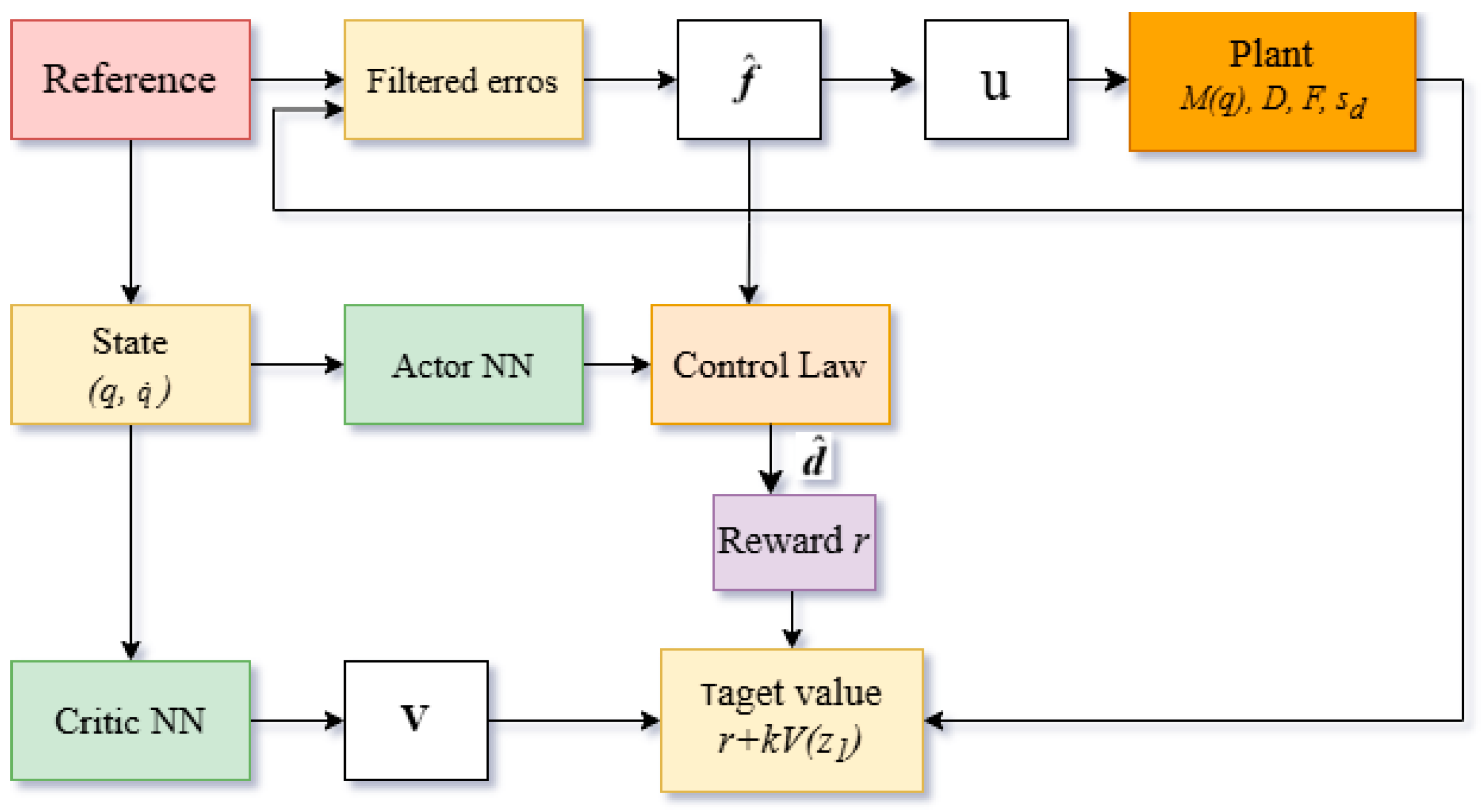
Figure 2 illustrates the overall DOB–ACRL control architecture used in this work. The main components are as follows:

Nominal controller block: This block computes a baseline torque command ${\mathit{\tau }}_{\mathrm{n}}(t)$ using the nominal model and the tracking error. It can be viewed as a conventional nonlinear or PD-like torque controller designed to achieve reasonable tracking performance in the absence of disturbances.

Disturbance observer (DOB) block: The DOB takes as input the measured joint states $q,\dot{q}$, the nominal control ${\mathit{\tau }}_{\mathrm{n}}$, and the plant output, and produces the disturbance estimate $\widehat{\mathit{d}}(t)$. This estimate is added to the nominal torque to compensate for the effect of $\mathit{d}(t)$, yielding a disturbance-compensated torque contribution.

Actor block: The actor is a neural network (or function approximator) that receives as input a state-related vector (typically including the error $z_1,z_2$ and possibly the DOB-related signals) and outputs an adaptive control component ${\mathit{\tau }}_{\mathrm{a}}(t)$. This adaptive component is combined with the nominal torque and disturbance compensation to form the final control input to the manipulator, $\mathit{\tau }(t)={\mathit{\tau }}_{\mathrm{n}}(t)+\widehat{\mathit{d}}(t)+{\mathit{\tau }}_{\mathrm{a}}(t)$, subject to actuator saturation.

Critic block: The critic approximates the value function or cost-to-go associated with the current policy. It takes as input the system state and error-related quantities and produces an estimate of the value function, which is used to compute the temporal difference (TD) error. The TD error drives the parameter updates in both the critic and actor networks.

Reward module block: The reward module computes the instantaneous reward signal based on three components: the tracking performance, energy usage, and control effort or torque smoothness. It also computes the normalized performance indicators and updates the corresponding reward weights online, implementing the adaptive multi-objective reward-shaping scheme described in Section 4. The resulting scalar reward is fed to the critic to update the value function.

In summary, the closed-loop DOB–ACRL system consists of the nominal controller and DOB providing a robust baseline, while the actor–critic and adaptive reward module refine the control law to improve the tracking, energy efficiency and torque smoothness. The key variables used in the subsequent Lyapunov analysis are: the state $\mathit{x}={[q^{\mathrm{T}};{\dot{q}}^{\mathrm{T}}]}^{\mathrm{T}}$, the tracking error and its derivative $z_1,z_2$, the disturbance estimate $\widehat{\mathit{d}}$, and the estimation error $\tilde{\mathit{d}}$. These variables will appear explicitly in the Lyapunov function candidate and in the derivation of stability and finite-time convergence conditions in Section 4.

4. Adaptive Reward Design and Lyapunov-Based Analysis

This section first introduces the proposed adaptive multi-objective reward-shaping scheme and then presents a Lyapunov-based stability analysis of the resulting DOB–ACRL closed-loop system.

4.1. Adaptive Multi-Objective Reward Shaping

In a conventional actor–critic R, the reward function is typically fixed throughout training, which can lead to suboptimal trade-offs when multiple objectives (tracking, energy, and smoothness) must be balanced online. To address this, we introduce three normalized performance indicators, $I_e(k),I_E(k),$ and $I_U(k)$ in $[0,1]$, and update the reward weights accordingly. By construction, $I_i(k)=0$ indicates good performance for objective $i, \mathrm{while} I_i(k)=1$ indicates poor performance.

Let $T_s$ be the sampling period and $N_w$ be the sliding window length. Define the windowed RMS tracking error as $e_{\mathrm{rms}}(k)=\sqrt{{\displaystyle \frac{1}{N_w}}{\displaystyle \sum _{j=k-N_w+1}^k\Vert e(}j){\Vert }_2^2},$ the window-averaged squared torque (energy proxy) as $\overline{E}(k)={\displaystyle \frac{1}{N_w}}{\displaystyle \sum _{j=k-N_w+1}^k\Vert \tau (j){\Vert }_2^2},$ and the window-averaged squared torque variation as $\overline{U}(k)={\displaystyle \frac{1}{N_w}}{\displaystyle \sum _{j=k-N_w+1}^k\Vert \Delta \tau (j){\Vert }_2^2},\hspace{1em}\hspace{1em}\Delta \tau (j)=\tau (j)-\tau (j-1).$ With the positive reference scales $e_{\mathrm{ref}},E_{\mathrm{ref}},\mathrm{and} U_{\mathrm{ref}}$ and the saturation operator ${\mathrm{sat}}_{[0,1]}(x)=\min (\max (x,0),1)$, the normalized indicators are defined as

$$\mathbf{I}(k)={[I_e(k),I_E(k),I_U(k)]}^{\top }={\left[{\mathrm{sat}}_{[0,1]}\left({\displaystyle \frac{e_{\mathrm{rms}}(k)}{e_{\mathrm{ref}}}}\right), {\mathrm{sat}}_{[0,1]}\left({\displaystyle \frac{\overline{E}(k)}{E_{\mathrm{ref}}}}\right), {\mathrm{sat}}_{[0,1]}\left({\displaystyle \frac{\overline{U}(k)}{U_{\mathrm{ref}}}}\right)\right]}^{\top }.$$

Given $\mathbf{I}(k)$, we compute the unnormalized preference scores using the exponential emphasis.

${\tilde{w}}_i(k)=\exp ({\lambda }_i{I}_i(k)), i\in \{e,E,U\},$ where ${\lambda }_i>0$ controls the sensitivity of each objective to its indicator. To avoid abrupt changes, we apply a first-order smoothing with the factor $\delta \in (0,1):$${\widehat{w}}_i(k)=(1-\delta )w_i(k-1)+\delta {\tilde{w}}_i(k).$ The sliding window length balances the responsiveness and noise: shorter windows react faster but are noisier, while longer ones yield smoother results with added delay. Similarly, the smoothing factor $\delta$ dictates the weight variation rates: a smaller $\delta$ facilitates rapid objective switching, whereas a larger $\delta$ ensures gradual transitions and smoother closed-loop behavior.

Finally, the weights are normalized to satisfy the simplex constraint $w_i(k)={\displaystyle \frac{{\widehat{w}}_i(k)}{{\widehat{w}}_e(k)+{\widehat{w}}_E(k)+{\widehat{w}}_U(k)}},\hspace{1em}\hspace{1em}{w}_e(k)+w_E(k)+w_U(k)=1, w_i(k)\ge 0$.

This adaptive reward scheduling increases the emphasis on the objectives with poorer recent performance, with a larger $I_i\left(k\right)$, while maintaining bounded and smooth weight evolution through (9). We consider three performance channels associated with the control objectives of the 2-DOF manipulator: a tracking performance term $r_t\left(t\right)$, an energy usage term $r_e\left(t\right)$, and a control smoothness (effort) term $r_c\left(t\right)$. The instantaneous tracking term $r_t\left(t\right)$ penalizes joint-position and velocity errors, for example, through a negative quadratic function of the error vector.

Remark (boundedness of adaptive reward weights): Because each indicator component is saturated into [0, 1], the exponential scores satisfy $\mathbf{1}\le {\tilde{w}}_i(k)\le \exp ({\lambda }_i)$. After smoothing and normalization, the weights remain non-negative and satisfy $w_e(k)+w_E(k)+w_U(k)=1$. Therefore, the weights are uniformly bounded and can be treated as bounded time-varying coefficients in the stability analysis. The smoothing factor δ further ensures that $w_i(k)$ varies gradually, avoiding discontinuities in the closed-loop dynamics.

$$z={[z_1^{\mathrm{T}} z_2^{\mathrm{T}}]}^{\mathrm{T}}$$

(6)

where $z_1=e=q-q_{\mathrm{d}}$ and $z_2=\dot{e}=\dot{q}-{\dot{q}}_{\mathrm{d}}$. The energy-related term $r_e(t)$ penalizes the instantaneous or short-horizon energy consumption, typically using the squared torques $\tau$ or the mechanical power. The control smoothness $r_c(t)$ penalizes rapid variations and large peaks in the control input, e.g., via the squared torque rate or a filtered measure of control effort. These three components are designed such that larger errors, higher energy usage or more aggressive control actions lead to lower reward values. To adapt the relative importance of these three objectives, we introduce the normalized performance indicators ${\varphi }_t(t),{\varphi }_e(t)$ and ${\varphi }_c(t)$, each taking values in [0, 1]. In particular, we define ${\varphi }_t(t)$ as a normalized measure of recent tracking performance, for instance, a moving-window root mean square (RMS) of the tracking error scaled by a reference value; ${\varphi }_e(t)$ as a normalized measure of recent energy usage, based on a moving average of instantaneous energy or torque squared; and ${\varphi }_e(t)$ as a normalized measure of recent control effort or torque smoothness, obtained from a moving average of torque variations or a similar quantity. By construction, $I_i(t)\in [0,1]$ quantifies the performance degradation: 0 = good and 1 = poor. The overall reward at time t is then computed as a weighted combination of the three components:

$$r\left(t\right)=w_t\left(t\right)r_t\left(t\right)+w_e\left(t\right)r_e\left(t\right)+w_c\left(t\right)r_c\left(t\right)$$

(7)

where $w_t\left(t\right)$, $w_e\left(t\right)$ and $w_c\left(t\right)$ are non-negative scalar weights satisfying the following: $w_t(t),w_e(t),w_c(t)\in [0,1],\hspace{1em}\forall t\ge 0$.

The weights are updated online according to the normalized performance indicators, implementing an adaptive multi-objective reward scheduling mechanism. A simple update rule is given by

$${\overline{\varphi }}_i(t+1)=(1-\beta ){\overline{\varphi }}_i(t)+\beta {\varphi }_i(t),\hspace{1em}i\in \{t,e,c\}$$

(8)

with a smoothing factor $\beta \in (0,1)$ followed by

$$w_i(t)={\displaystyle \frac{{\tilde{w}}_i(t)}{{\tilde{w}}_t(t)+{\tilde{w}}_e(t)+{\tilde{w}}_c(t)}}$$

(9)

This normalization guarantees that the weights always sum to one and remain within [0, 1]. The rule has an intuitive interpretation: when the tracking performance is poor (large ${\varphi }_t$), the tracking term dominates the overall reward and the learning updates prioritize policies that rapidly reduce the error; when the tracking has improved but the energy usage or torque variations are high (large ${\varphi }_e$ or ${\varphi }_c$), the corresponding weights increase, encouraging the policy to reduce energy consumption and produce smoother control actions while maintaining acceptable tracking. Overall, this adaptive weighting mechanism allows for the DOB–ACRL controller to dynamically make trade-offs among fast and accurate tracking, energy efficiency and smooth control effort, rather than relying on a single, hand-tuned set of fixed weights. We emphasize that this is an adaptive multi-objective reward-shaping scheme: the reward structure is adjusted online according to performance, rather than being a static, policy-invariant transformation of a fixed cost.

4.2. Assumptions and Lyapunov Function

In addition to Assumptions 1 and 2 regarding bounded disturbance and bounded parameter uncertainty, stated in Section 3, we introduce the following assumptions for the stability analysis.

Assumption 3

(regularity of dynamics). The nominal dynamics of the manipulator are locally Lipschitz in the state  $x$ and piecewise continuous in time. The closed-loop error dynamics with the nominal controller and DOB are well defined and forward complete on any compact subset of the state space.

Assumption 4

(bounded approximation errors). The critic and actor neural networks approximate the ideal value function and control policy with bounded errors. Specifically, there exist constants ${\epsilon }_c>0$ and  ${\epsilon }_a>0$ such that the approximation errors of the critic and actor satisfy:

$$\Vert {\epsilon }_c(x)\Vert \le {\epsilon }_c,\hspace{1em}\Vert {\epsilon }_a(x)\Vert \le {\epsilon }_a,\hspace{1em}\forall x\in D$$

(10)

where  $\mathcal{D}$ is a compact operating region containing the trajectories of interest.

Assumption 5

(bounded DOB estimation error). The disturbance observer is designed such that the estimation error  $\tilde{d}(t)=d(t)-\widehat{d}(t)$ is bounded, i.e., there exists  ${\tilde{d}}_{\max }>0$ with  $\Vert \tilde{d}(t)\Vert \le {\tilde{d}}_{\max },\forall t\ge 0$.

Assumption 6

(bounded control and saturation). The actuator saturation levels are finite and the saturated control input remains bounded for all time. Moreover, the actor updates and nominal controller gains are chosen such that the resulting torque commands do not drive the system outside the compact region $D$. To analyze the closed-loop stability, we define the following error-related quantities.

Let

$$z=\left[\begin{array}{c}{z}_1\\ z_2\end{array}\right]=\left[\begin{array}{c}e\\ \dot{e}\end{array}\right]$$

(11)

denote the tracking error state, and let ${\tilde{\theta }}_c$ and ${\tilde{\theta }}_a$ represent the parameter estimation errors of the critic and actor networks, respectively, with respect to their ideal parameters. The disturbance estimation error $\tilde{d}$ is defined above.

A composite Lyapunov candidate is chosen as

$$V(z,{\tilde{\theta }}_c,{\tilde{\theta }}_a)=V_z(z)+V_c({\tilde{\theta }}_c)+V_a({\tilde{\theta }}_a)$$

(12)

where

$$V_z(z)={\displaystyle \frac{1}{2}}{z}^{\mathrm{T}}Pz$$

(13)

for some symmetric positive definite matrix P, and

$$V_c({\tilde{\theta }}_c)={\displaystyle \frac{1}{2}}{\tilde{\theta }}_c^{\mathrm{T}}{\Gamma }_c^{-1}{\tilde{\theta }}_c,\hspace{1em}{V}_a({\tilde{\theta }}_a)={\displaystyle \frac{1}{2}}{\tilde{\theta }}_a^{\mathrm{T}}{\Gamma }_a^{-1}{\tilde{\theta }}_a$$

(14)

with positive definite adaptation gain matrices ${\Gamma }_c,{\Gamma }_a$. The choice of adaptation laws for the critic and actor (driven by the temporal difference error) is made such that the cross terms between the parameter errors and TD error are canceled or dominated in $\dot{V}$, as is standard in actor–critic Lyapunov analyses.

Actor–critic update laws (used in the Lyapunov analysis): To make the argument in Equation (15) explicit, we consider the standard TD error-driven continuous-time adaptation laws (a continuous-time approximation of the discrete updates in Section 5.1). Let the TD error be

$$\begin{array}{l}\delta (t)=r(t)+\gamma \widehat{V}(z(t+\Delta t))-\widehat{V}(z(t))\\ {\dot{\theta }}_c=-{\Gamma }_c{\sigma }_c(z)\delta (t),\\ {\dot{\theta }}_a=-{\Gamma }_a{\sigma }_a(z)\delta (t)\end{array}$$

(15)

where ${\sigma }_c(z)$ and ${\sigma }_a(z)$ denote the critic–actor regression (or backpropagated sensitivity) vectors, and ${\Gamma }_c,{\Gamma }_a$ are the positive definite gains. With these choices, the cross-terms between the parameter errors and the TD error appearing in $V$ are canceled or upper-bounded by quadratic terms, which yields the compact bound in Equations (15) and (16) under Assumption 4.

Taking the time derivative of V along the trajectories of the DOB–ACRL closed-loop system, and using the nominal error dynamics, the DOB compensation, the bounded disturbance and approximation errors, and the actor and critic update laws, we obtain an inequality of the form

$$\dot{V}\le -c_1\Vert z{\Vert }^2+c_2\Vert z\Vert \Vert {\epsilon }_a(x)\Vert +c_3\Vert {\epsilon }_c(x){\Vert }^2+c_4\Vert \tilde{d}(t){\Vert }^2$$

(16)

for positive constants $c_1,c_2,c_3,c_4$ that depend on the system and controller parameters.

By applying Assumptions 4 and 5, we can bound the error terms uniformly and write

$$\dot{V}\le -{\alpha }_1\Vert z{\Vert }^2+{\alpha }_2$$

(17)

for some ${\alpha }_1>0$ and ${\alpha }_2\ge 0$. Since $V_z(z)$ is quadratic and positive definite, there exist constants $\underset{\_}{\lambda },\overline{\lambda }>0$ such that

$$\underset{\_}{\lambda }\Vert z{\Vert }^2\le V_z(z)\le \overline{\lambda }\Vert z{\Vert }^2$$

(18)

which allows us to rewrite the bound on $\dot{V}$ in terms of V, yielding an inequality of the type

$$\dot{V}\le -k_{1}V+k_2$$

(19)

for suitable positive constants $k_1$ and $k_2$. This inequality serves as the basis for establishing the uniform ultimate boundedness of the tracking error and parameter estimates.

4.3. Stability Results and Finite-Time Remark

Theorem 1

(uniform ultimate boundedness of the DOB–ACRL closed loop). Under Assumptions 1–6, and for sufficiently small learning rates of the actor and critic networks and appropriate choices of the nominal controller and DOB gains, there exist positive constants k₁ and k₂ such that the composite Lyapunov function $V(z,{\tilde{\theta }}_c,{\tilde{\theta }}_a)$ satisfies

$$\dot{V}\le -k_{1}V+k_2.V$$

(20)

Consequently, all the closed-loop signals remain bounded, and the tracking error vector

$$z(t)={[e^{\mathrm{T}}(t) {\dot{e}}^{\mathrm{T}}(t)]}^{\mathrm{T}}$$

(21)

is uniformly ultimately bounded. In particular, there exists a finite radius  $r$ > 0 such that  $\underset{t\to \infty }{\lim \sup }‖z(t)‖\le r$, where  $r$ depends on the bounds of the disturbance, the DOB estimation error, and the approximation errors of the actor and critic networks.

Proof. 

The inequality $\dot{V}\le -k_{1}V+k_{2}V$ implies that V(t) converges exponentially to a compact set whose size is proportional to  $k_2/k_1$. Standard comparison lemma arguments show that

$$V(t)\le V(0)e^{-k_{1}t}+{\displaystyle \frac{k_2}{k_1}}\left(1-e^{-k_{1}t}\right)$$

(22)

from which the uniform ultimate boundedness of $V$ and hence of z, ${\tilde{\theta }}_c$ and ${\tilde{\theta }}_a$ follows. □

Remark 1

(finite-time convergence in ideal conditions). If, in addition to Assumptions 1–6, the approximation errors and DOB estimation error vanish (i.e., $a=0,c=0,\tilde{\mathit{d}}(t)\equiv 0$), then the inequality for $\dot{V}$ can be strengthened to a nonlinear form $\dot{V}\le -kV$ for some $k>0$ and $\gamma \in (0,1)$, in line with the analysis in [37]. Integrating this inequality yields an upper bound on the finite convergence time for $V(t)$, and thus for the tracking error. In practice, however, nonzero approximation and disturbance-estimation errors prevent exact finite-time stabilization, and the system exhibits practical finite-time convergence to a small residual set rather than the origin. The main theoretical guarantee of the present work is therefore the UUB of the DOB–ACRL closed loop, with the finite-time behavior serving as an additional insight under idealized assumptions.

5. Simulation Evaluation

5.1. Simulation Setup and Implementation Details

To validate the theoretical developments and assess the practical performance of the proposed DOB–ACRL controller, a series of numerical simulations were conducted on a 2-DOF robotic manipulator. The manipulator dynamics followed the nonlinear model introduced in Section 3, with parameters as shown in

Table 1. Robot manipulator parameters.

Parameter	Symbol	Value	Unit
Inertia coefficient 1	$p_1$	3.473	Kg·m2
Inertia coefficient 2	$p_2$	0.196	kg·m2
Inertia coefficient 3	$p_3$	0.242	kg·m2
Joint 1 friction	$f_{d1}$	5.3	N·m·s
Joint 2 friction	$f_{d2}$	1.1	N·m·s
Link length 1	$l_1$	0.5	m
Link length 2	$l_2$	0.5	m

.

The control objective was to track the smooth reference trajectories of the form $y_{r,i}(t)=\left(1-e_t\right)\sin {\omega }_{i}t$, with frequencies ${\omega }_1=0.5\left(\mathrm{rad}/\mathrm{s}\right)$ and ${\omega }_2=0.75\left(\mathrm{rad}/\mathrm{s}\right)$. To emulate the realistic uncertainties, the system was subjected to mixed disturbances consisting of sinusoidal, step, and stochastic components $d_i(t)=0.2\sin (2t)+0.1\mathrm{sign}(\sin (0.5t))+0.05\mathrm{randn}(t)$, representing the dynamic friction, external shocks, and measurement noise.

This subsection summarizes the main implementation details of DOB–ACRL controller to facilitate reproducibility.

(a)

Actor network: The actor is implemented as a feedforward neural network with two hidden layers. The input vector consists of the tracking error and its derivatives $z_1=e=q-q_{\mathrm{d}}$ and $z_2=\dot{e}=\dot{q}-{\dot{q}}_{\mathrm{d}}$. The proposed neural network architecture consists of four distinct layers. The network begins with an input layer comprising four neurons, which receive the normalized error states of the system. Following the input, there are two consecutive hidden layers. Hidden layer 1 contains 64 neurons and utilizes the ReLU activation function and, similarly, hidden layer 2 also has 64 neurons and employs the ReLU activation function. Finally, the network concludes with the output layer, which consists of two neurons using a linear activation function corresponding to the adaptive torque components ${\tau }_{\mathrm{a}}\in R^2$. The final torque command is obtained by combining the nominal control, the DOB compensation and the actor output, and then applying saturation to respect the actuator limits.

(b)

Critic network: The critic network serves to approximate the state-value function $V(z)$. It utilizes the same input vector as the actor network, which comprises the system’s state information. The critic’s structure is defined by its layers: it features an input layer of four neurons, followed by two consecutive hidden layers, each containing 64 neurons and employing the ReLU activation function. The network concludes with an output layer consisting of a single neuron with a linear activation, which provides the scalar value estimate $\widehat{V}(z)$. The crucial TD error is then computed by comparing this critic output with the reward provided by the adaptive reward module. This TD error is subsequently used as the training signal to update the parameters of both the critic and the actor networks.

(c)

Learning rates and discount factor: The critic and actor parameters are updated online using gradient-based rules driven by the TD error. The learning rates are chosen as the critic learning rate ${\alpha }_c=1.0\times {10}^{-3}$ and the actor learning rate ${\alpha }_a=5.0\times {10}^{-4}$, and the discount factor is set to $\gamma =0.99$. These values are selected to ensure a compromise between the convergence speed and numerical stability of the learning process.

Discrete-time implementation detail: All the learning updates are performed in discrete time. At each time step k, we compute the TD error: ${\delta }_k=r_k+\gamma \widehat{V}(z_{k+1})-\widehat{V}(z_k)$ and minimize the squared TD loss $L_k={\displaystyle \frac{1}{2}}{\delta }_k^2$. The critic parameters ${\theta }_c$ are updated by gradient descent ${\theta }_c(k+1)={\theta }_c(k)-{\alpha }_c{\displaystyle \frac{\partial L_k}{\partial {\theta }_c}}$. The actor is updated using the critic as a baseline (deterministic policy gradient and backprop through the torque output) to maximize $V$, i.e., ${\theta }_a(k+1)={\theta }_a(k)+{\alpha }_a{\displaystyle \frac{\partial \widehat{V}(z_k)}{\partial {\theta }_a}}$. The continuous-time Lyapunov analysis in Section 4 can be viewed as an approximation of these discrete updates that becomes accurate when the sampling period $\Delta t$ and learning rates are sufficiently small. In practice, stability and boundedness are promoted by small learning rates, bounded reward weights (Section 4.1), and input saturation, which together justify treating the learning terms as bounded perturbations in the UUB argument. Smaller learning rates enhance numerical stability and reduce TD loss oscillations but slow convergence; conversely, larger rates accelerate learning at the risk of overshoot and instability under disturbances. Similarly, a larger discount factor prioritizes long-term performance, while a smaller value emphasizes immediate error reduction, increasing speed but potentially inducing oscillations.

(d)

Simulation horizon and episodes: All simulations are carried out in discrete time with a fixed sampling period of $\Delta t=1 \mathrm{m}\mathrm{s}$. Each episode has a duration of $T_{\mathrm{ep}}=10 \mathrm{s}$ corresponding to 10,000 time steps per episode. Unless otherwise stated, the results reported in Section 5 were obtained after 200 training episodes, which were sufficient for the TD error and performance indices to reach a steady regime in all tested configurations.

(e)

Numerical integration: The continuous-time manipulator dynamics are integrated using a fourth-order Runge–Kutta (RK4) scheme with the step size $\Delta t=1 \mathrm{m}\mathrm{s}$ matching the control update period. At each integration step, the torque command is held constant, and the DOB, actor and critic are updated based on the most recent state and reward.

(f)

Network initialization: All network weights and biases for the actor and critic are initialized using a zero-mean Gaussian distribution with a standard deviation of 0.01, and the biases are initialized to zero. Before training, the input states are normalized by fixed scaling factors corresponding to the maximum expected ranges of $q$, $\dot{q}$ and the tracking errors. No pre-training or offline learning is used; all the parameter updates are performed online during interaction with the simulated manipulator.

These implementation choices are found to provide stable learning behavior across the considered scenarios for the 2-DOF manipulator and are kept identical for the proposed DOB–ACRL controller and the two baseline controllers to allow for fair comparison. Additionally, since the core objective of this study is to isolate and quantify the impact of reward design on control performance, we focus our comparisons on two scenarios within the same actor–critic framework—a fixed reward versus an adaptive (time-varying) reward weighting—so that the observed differences can be attributed specifically to the reward function variation rather than to structural differences among the controllers.

5.2. Simulation Process

5.2.1. Numerical Simulation Case 1: Mode A—AC (Static Reward)

In this mode, a conventional AC controller is implemented using a fixed quadratic reward function: $r_t^{base}=-z_1^T\mathit{Q}{z}^T-{\mathit{u}}^T\mathit{R}\mathit{u}$.

The simulation loop proceeds as follows:

Step 1. Compute the tracking errors $z_1^{\top },z_2^{\top }$.

Step 2. The actor network estimates $\widehat{\mathit{f}}(.)$; no DOB is used.

Step 3. The control torque is generated as $\mathit{u}=\mathit{M}(q)({\ddot{\mathit{y}}}_r-k_1{z}_1-k_2{z}_2-\widehat{\mathit{f}}(x))$.

Step 4. The manipulator dynamics are integrated using a fourth-order Runge–Kutta method.

Step 5. The fixed reward is calculated, and the critic and actor networks are updated based on the temporal difference (TD) loss.

Expected behavior: Slow learning, possible convergence to local minima under disturbances, and limited coordination between accuracy and energy efficiency.

5.2.2. Numerical Simulation Case 2: Mode B—AC (Actor–Critic with the Adaptive Composite Reward Without Disturbance Observer)

In this mode, the proposed DOB–ACRL with adaptive composite reward and DOB compensation as formulated in Equations (8) and (9) is implemented. At each time step:

Step 1. Calculate the instantaneous performance indices ${\varphi }_i\left(t\right)$(RMS error, energy, and effort).

Step 2. Update the adaptive weights $w_t,w_c,w_e$.

Step 3. Compute the composite reward r_t and update both networks.

Expected behavior: Faster convergence and improved tracking compared to Mode A, but residual oscillations remain under strong disturbances due to the absence of a DOB.

5.2.3. Numerical Simulation Case 3: Mode C-DOB–ACRL (Adaptive Reward + DOB)

This configuration combines the adaptive reward with a DOB to form the proposed DOB–ACRL framework.

The DOB is formulated as

$$\dot{\mathit{h}}=-\alpha (\mathit{h}+\alpha \dot{\mathit{q}})-\alpha (\widehat{\mathit{f}}(x)+\mathit{u}),\widehat{\mathit{d}}=\mathit{h}+\mathit{\alpha }\dot{\mathit{q}}$$

(23)

The control law becomes

$$\mathit{u}=\mathit{M}(\mathit{q})({\ddot{\mathit{y}}}_r-k_1{z}_1-k_2{z}_2-\widehat{\mathit{f}}(x)-\widehat{\mathit{d}})$$

(24)

Simulation steps:

Step 1. Compute $z_1,z_2$ and the actor output $\widehat{\mathit{f}}(x)$.

Step 2. Update the DOB to estimate the disturbance $\widehat{\mathit{d}}\left(t\right)$.

Step 3. Apply the control torque $u$ as above.

Step 4. Integrate the system dynamics and update the reward weights and TD losses.

Expected behavior: Fastest convergence, superior robustness against noise and parameter uncertainty, and optimal energy–effort balance.

Equation (23) is the discrete-time implementation of the DOB formulated in Section 3: at each sampling step, ${\widehat{d}}_{k+1}$ is updated using the same disturbance reconstruction term derived from the nominal dynamics and measured and control signals. In the simulations, $\ddot{q}$ is obtained from the numerical differentiation of $\dot{q}$ and then passed through a low-pass filter to reduce noise before being used in the DOB update.

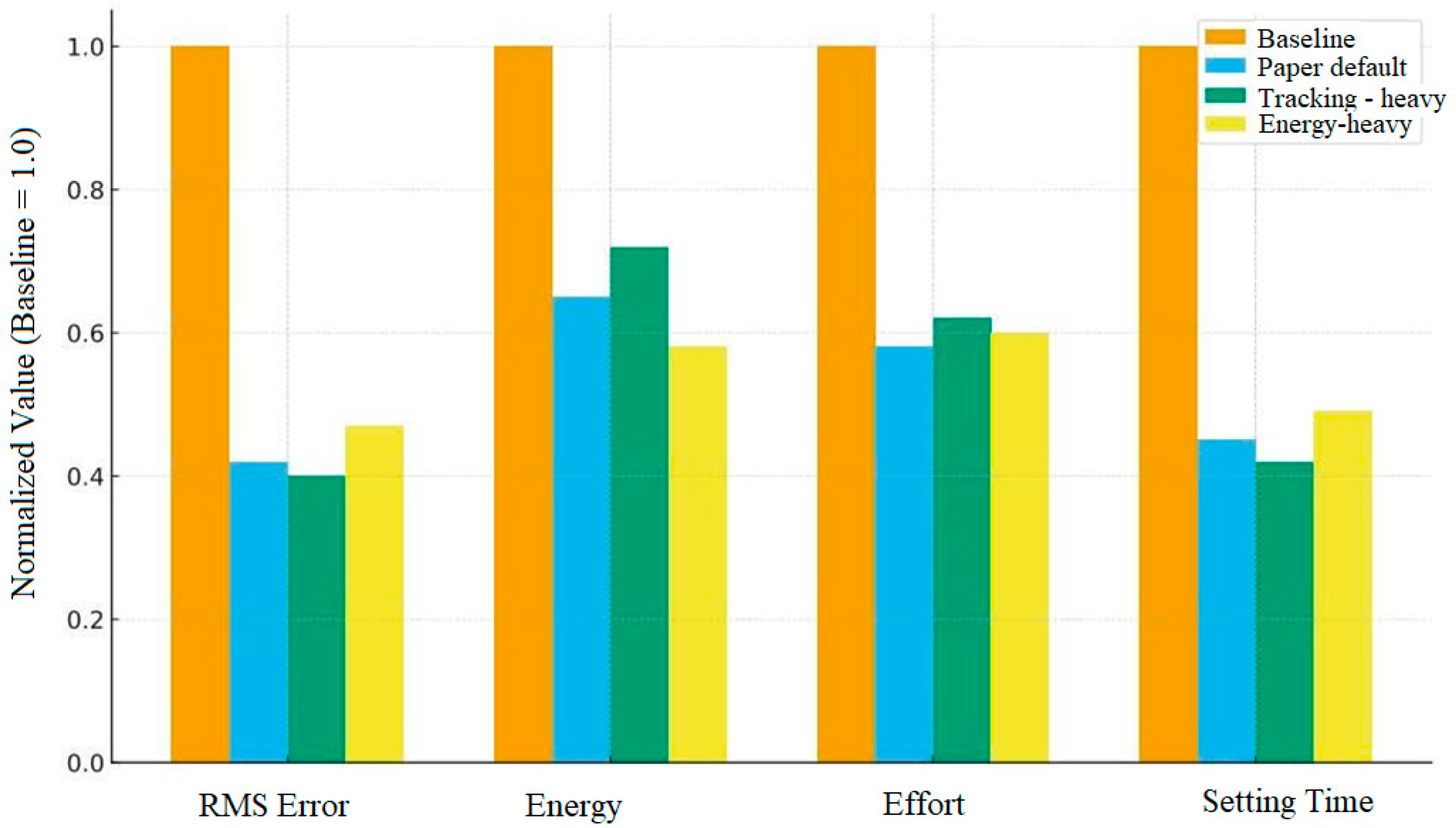
To investigate the sensitivity of the adaptive reward mechanism, a parameter sweep is conducted for the exponential scaling coefficients ${\beta }_t,{\beta }_c,{\beta }_e$ and initial weight distributions $w_{t_0},w_{c_0},w_{e_0}$. The table below summarizes the illustrative results (normalized with respect to the static baseline, mode $A$).

Table 2. Reward parameter variation study.

Mode	Scenario	${\mathit{\beta }}_{\mathit{t}}$	${\mathit{\beta }}_{\mathit{c}}$	${\mathit{\beta }}_{\mathit{e}}$	${\mathit{w}}_{{\mathit{t}}_0}$	${\mathit{w}}_{{\mathit{c}}_0}$	${\mathit{w}}_{{\mathit{e}}_0}$	Notes
A	Baseline (fixed)	1.0	1.0	1.0	0.60	0.25	0.15	Adaptive reward only
B	Adaptive (no DOB)	1.0	1.0	1.0	0.70	0.20	0.10	Default configuration
C	Proposed (DOB + ACRL)	+2.0	0.7	0.7	0.80	0.15	0.05	High accuracy, higher energy
C	Tracking heavy	0.7	2.0	1.0	0.55	0.35	0.10	Energy savings, mild error
C	Energy heavy	0.8	1.0	2.0	0.55	0.20	0.25	Smoother torques
C	Effort heavy	2.5	2.5	2.5	0.70	0.20	0.10	Fastest learning, risk of oscillation
C	Aggressive adaptation	0.5	0.5	0.5	0.70	0.20	0.10	Slower but stable
C	Conservative adaptation	1.0	1.0	1.0	0.60	0.25	0.15	Adaptive reward only

displays the control trade-offs governed by the reward-scheduling parameters. A higher tracking sensitivity reduces the RMS error but increases the energy consumption, while the ‘energy-heavy’ and ‘effort-heavy’ settings prioritize lower torque magnitude or smoothness at the expense of transient performance. The adaptation coefficients determine the response speed: aggressive settings accelerate learning but may induce oscillations, whereas conservative settings prioritize stability. These results confirm the efficacy of the intended multi-objective adaptive reward design.

This section defines the performance metrics used to evaluate the proposed method. The performance was quantitatively evaluated using four key indices. Root mean square (RMS) tracking error:

$${\mathrm{RMS}}_i=\sqrt{{\displaystyle \frac{1}{T}}{\displaystyle {\int }_0^T{z}_{1,i}^2}(t)dt}, \mathrm{RMS}={\displaystyle \frac{1}{2}}({\mathrm{RMS}}_1+{\mathrm{RMS}}_2)$$

(25)

Control energy consumption:

$$\mathit{E}={\displaystyle \underset{o}{\overset{T}{\int }}\Vert \mathit{u}(t){\Vert }_2^{2}dt}$$

(26)

Average control effort:

$$\mathit{U}={\displaystyle \frac{1}{T}}{\displaystyle {\int }_o^T{\Vert \mathit{u}(t)\Vert }_1 dt}$$

(27)

Settling time: The time at which both joint errors satisfy $|z_{1,i}(t)|<0.05, \forall t\ge T_s$ and remain within this bound for 0.5 s. These metrics together capture the precision, efficiency, and smoothness, forming the basis for the adaptive reward transformation.

The bar plot in Figure 3 quantitatively illustrates the performance differences for all metrics. The DOB + ACRL configuration outperforms the static baseline in every aspect, confirming that adaptive reward weighting and DOB synergy lead to superior tracking precision, smoother torque profiles, and reduced control energy.

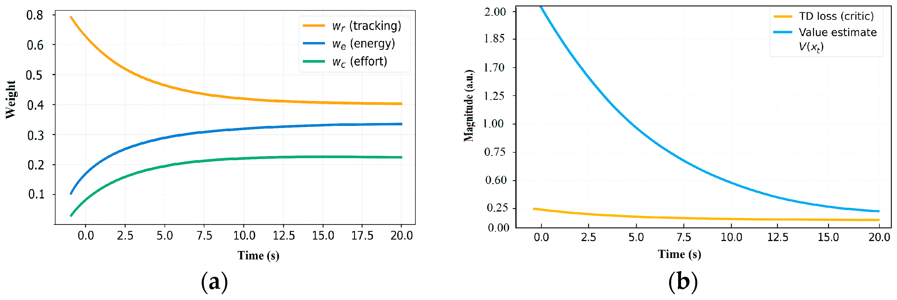
Figure 4a shows the evolution of the adaptive reward weights. The weighting gradually shifts from tracking dominant to a more energy- and effort-aware allocation as the controller performance improves, reflecting the intended online weight scheduling behavior in Equations (8) and (9). Figure 4b reports the TD loss evolution, which exhibits a stable decay with small residual fluctuations, indicating the improved training stability of the actor–critic update.

5.3. Results

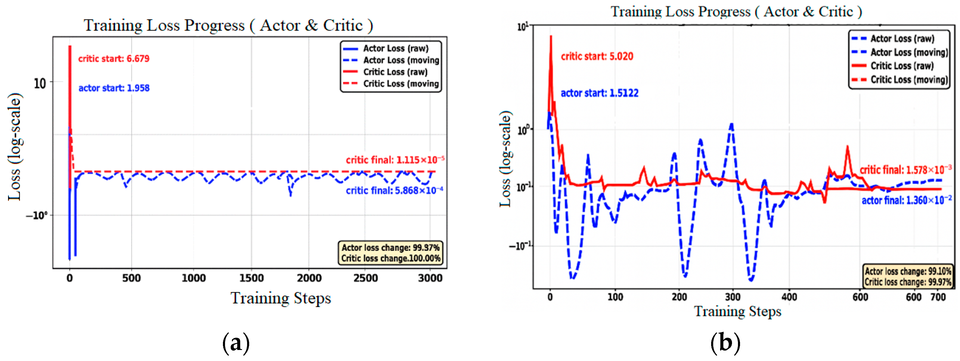
To further validate the theoretical findings presented in Section 4, this subsection analyzes the learning convergence behavior of the proposed DOB–ACRL framework by examining the evolution of the critic TD loss and the value function trajectories during training. Figure 5 depicts the TD loss profiles for the three control configurations: baseline AC with static reward, adaptive reward AC (without DOB), and DOB–ACRL (proposed).

In the adaptive reward AC case, shown in Figure 4a, although the proposed DOB–ACRL framework significantly reduces the tracking error, the actor shows small residual oscillations in the steady regime. These minor fluctuations are attributed to the remaining approximation errors and the high-frequency components of the mixed disturbances that are not fully eliminated by the learning process. With DOB–ACRL (Figure 5b), convergence is faster and smoother: both losses decrease by several orders of magnitude with nearly monotonic, noise-free curves, indicating that the disturbance observer effectively suppresses the disturbance effects and stabilizes learning.

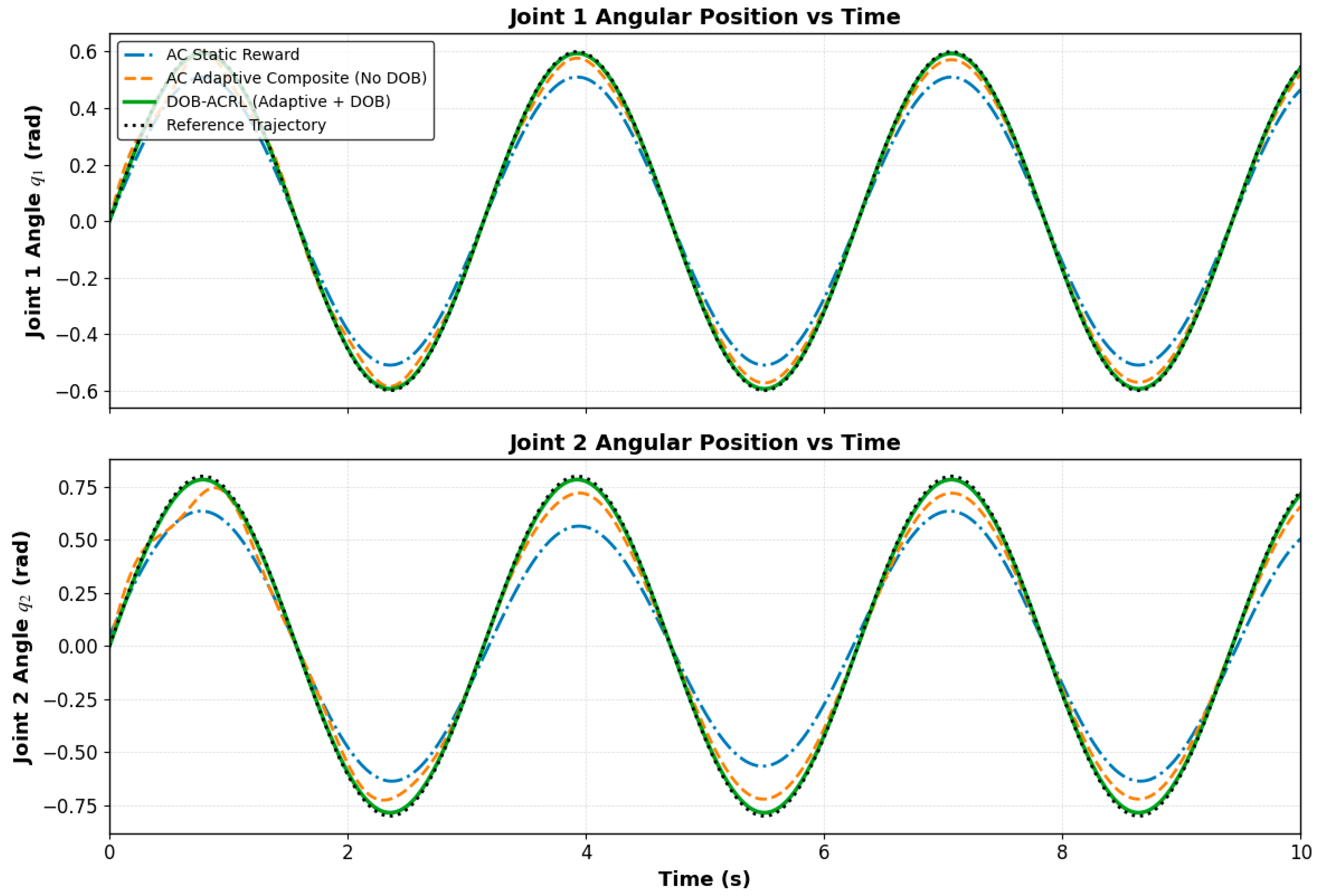
Figure 6 shows that all three methods track the sinusoidal references, but DOB–ACRL (green) almost overlaps the reference for both joints, yielding the smallest phase lag and amplitude error most noticeably on $q_2$. Quantitatively (from the plotted traces), the steady-state deviation is only on the order of a few ${10}^{-2}$ rad for DOB–ACRL, whereas AC Static exhibits a visibly larger peak and valley mismatch (typically several ${10}^{-2}$ rad, with the largest discrepancy occurring on $q_2$), and AC Adaptive without DOB provides only a marginal reduction compared with AC Static.

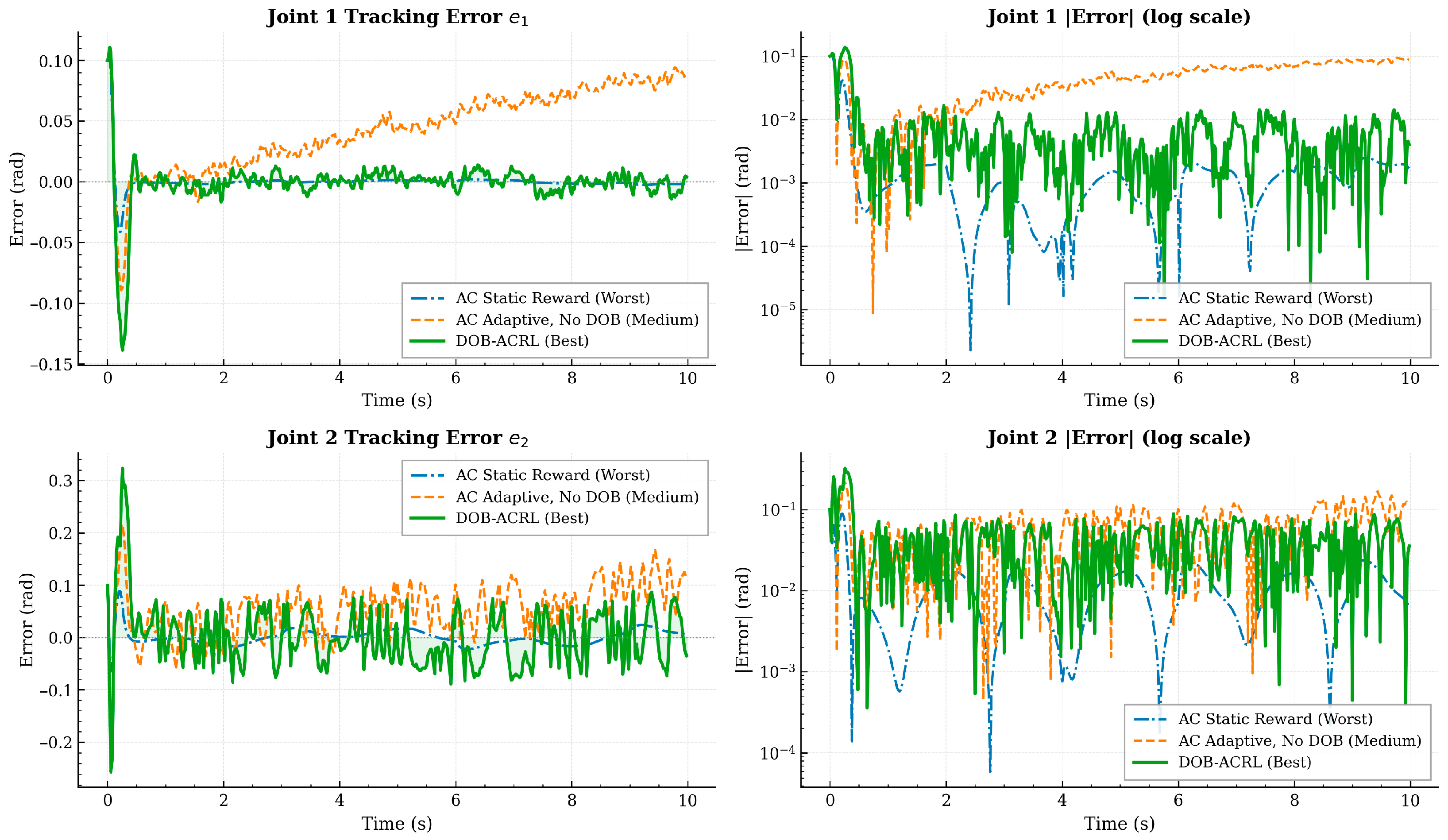
The figure indicates that DOB–ACRL (green) achieves the smallest and most stable tracking errors after the initial transient. In particular, for joint $q_2$, the steady-state error amplitude is approximately $\pm (0.04-0.06)rad$ with DOB–ACRL, compared with $\pm (0.06-0.08)rad$ for AC Adaptive without DOB, and up to about $\pm (0.12-0.16)rad$ for AC Static at peak deviations. For joint $q_1$, the errors are smaller overall for all methods, but DOB–ACRL still shows the lowest oscillation around zero in a steady state.

The joint tracking performance of the 2-DOF planar manipulator is presented in Figure 7, highlighting that the proposed DOB-ACRL controller achieves the best tracking accuracy compared to the AC Static Reward and AC Adaptive (No DOB) methods.

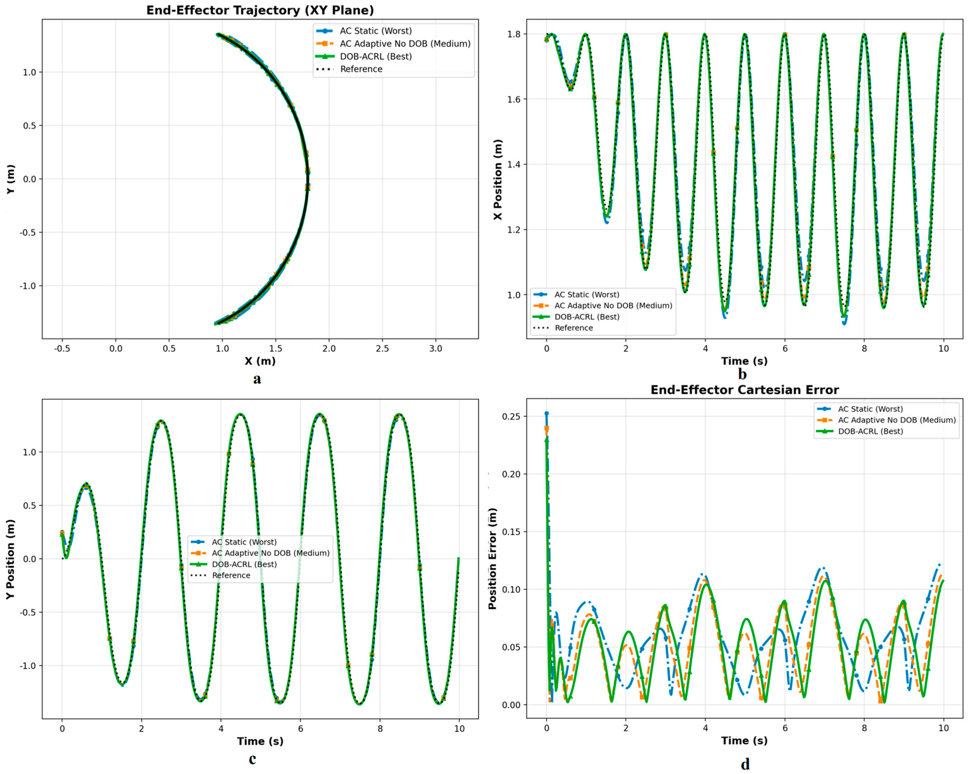
Figure 8 compares the tracking performance of the three methods. The DOB–ACRL controller follows the semicircular trajectory most closely, with the x and y profiles matching the references and the peak errors staying below 0.02 m. The position error converges within 2 s and remains bounded over 15 s, demonstrating its superior accuracy and robustness compared to the two baselines.

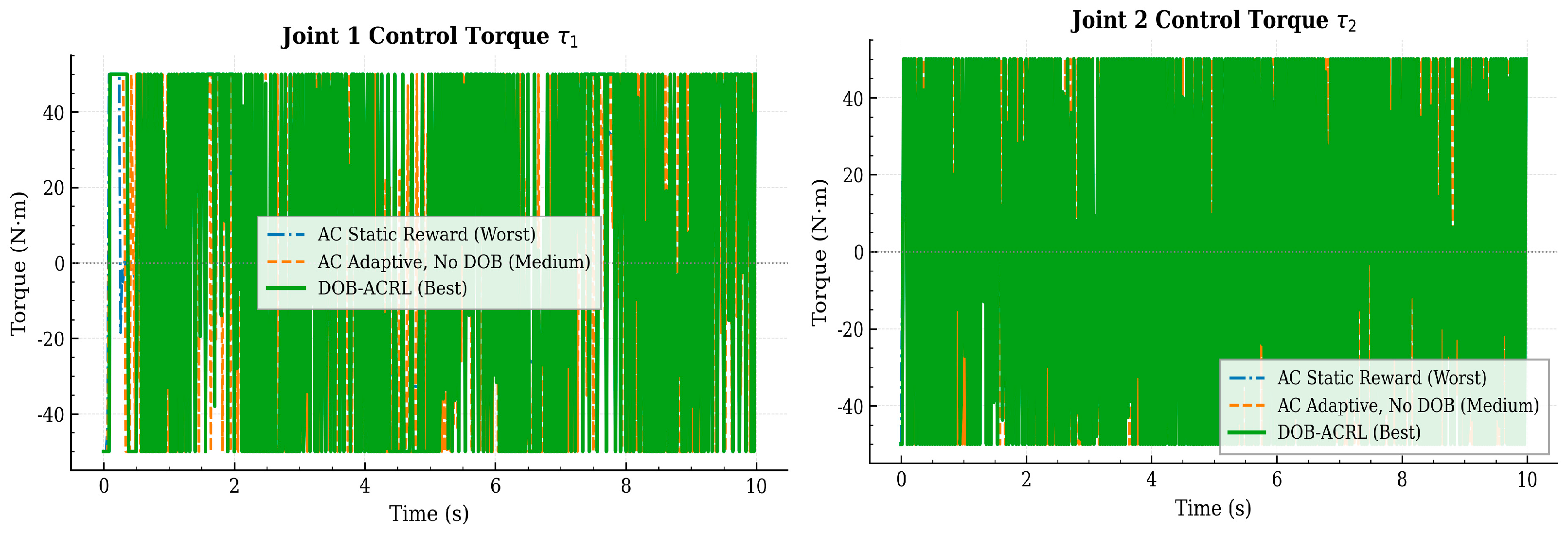
Figure 9 compares the resulting joint torque commands ${\tau }_1$ and ${\tau }_2$ generated by the three controllers while tracking the same sinusoidal reference trajectory.

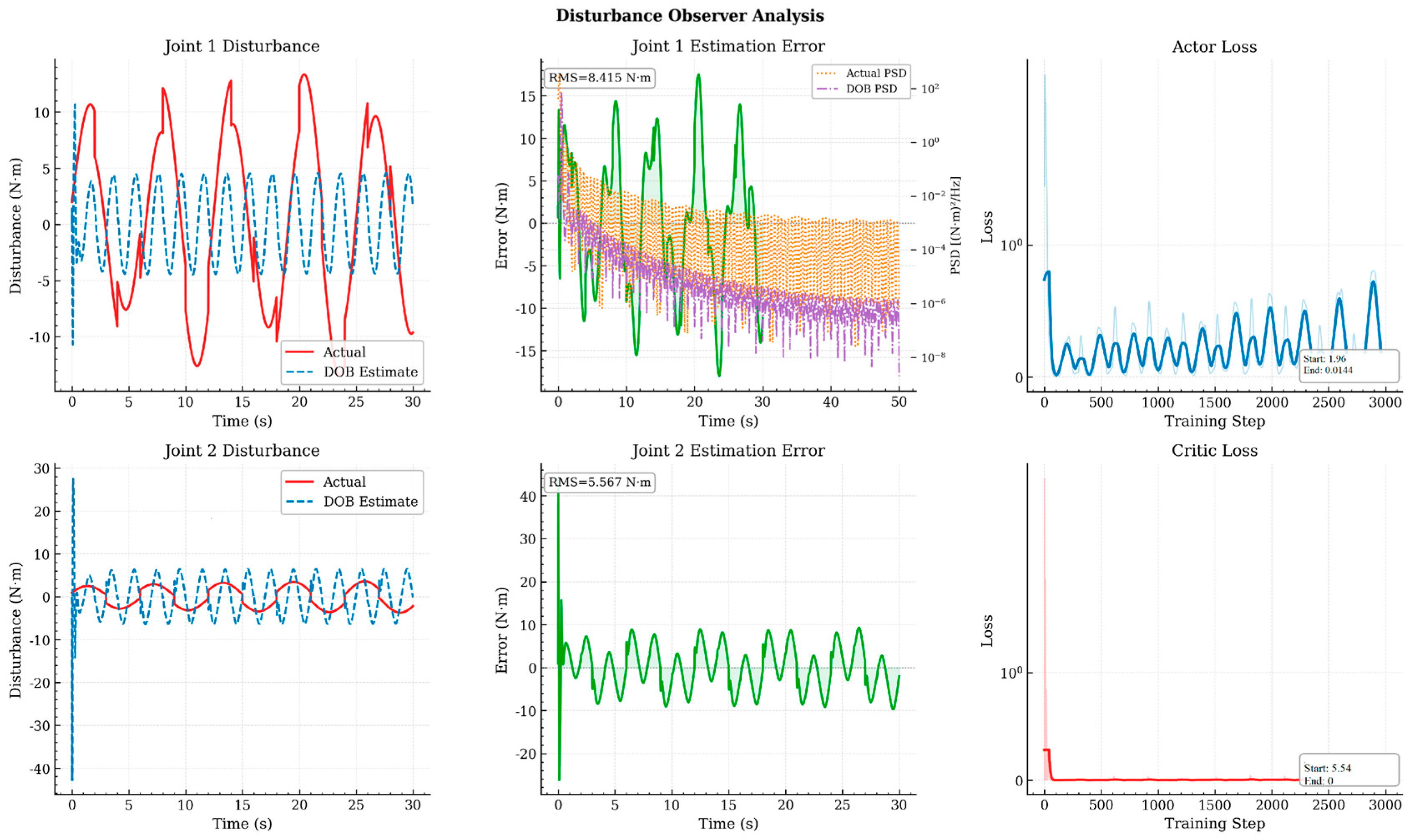
Figure 10 shows the disturbance estimation and learning performance under the proposed DOB–ACRL controller. The DOB provides accurate disturbance reconstruction, which improves the closed-loop robustness and yields more stable learning signals in the presence of external perturbations and varying loads. The actor and critic loss curves demonstrate stable convergence; specifically, the critic loss reaches near zero within the first 200 iterations, while the actor loss stabilizes significantly after approximately 1500–2000 training steps.

The quantitative performances of the compared controllers are summarized in

Table 3. Summary of the quantitative performance of the compared controllers.

Case	RMS e1	RMS e2	Avg. Control Effort	Max EE Error (m)	Settling Time (s)
Case 1: AC (static reward)	0.0139	0.0809	10.4380	0.2525	0.65
Case 2: AC (actor–critic with an adaptive composite reward without a disturbance observer)	0.0132	0.0358	10.8923	0.2399	0.54
Case 3: DOB–ACRL (adaptive reward + DOB)	0.0137	0.0274	10.9185	0.2299	0.34

.

Based on Table 3, the proposed DOB–ACRL achieves the best overall performance: it reduces the RMS of $e_{q2}$ to 0.0274 rad and the Max EE error to 0.2299 m. These results demonstrate that the inclusion of DOB significantly improves the tracking accuracy and reduces the end-effector errors. In contrast, AC Adaptive shows a notable improvement over AC Static only in $e_{q2}$ (0.0358 vs. 0.0809 rad). Meanwhile, the RMS of $e_{q1}$ remains nearly identical across all methods (0.0132–0.0139 rad), and the differences in the avg. control effort are marginal, with AC Static recording the lowest value (10.4380).

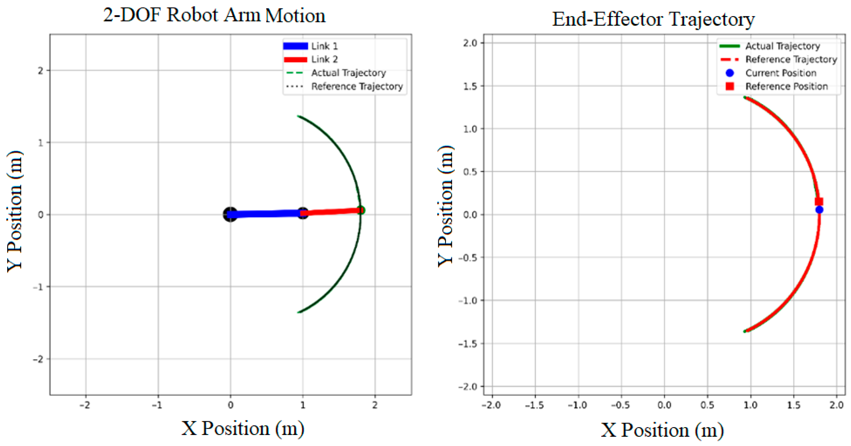
Figure 11 illustrates the 2-DOF manipulator motion and end-effector tracking under DOB–ACRL. The actual end-effector path closely follows the semicircular reference, and the zoomed view shows only small deviations, confirming accurate spatial tracking and smooth, consistent motion.

6. Discussion and Implications

This section discusses the proposed DOB–ACRL controller in terms of its three main design objectives: tracking optimality, energy efficiency, and sustainability in the sense of smooth control effort. It situates the approach within the existing literature and highlights the limitations and future directions. The results confirm that adaptive reward scheduling optimizes the control trade-off by balancing the transient tracking accuracy with energy efficiency, while the DOB improves robustness against lumped disturbances. However, as these findings are based on 2-DOF simulations with limited disturbance profiles, future work will focus on hardware validation, higher-DOF systems, and broader benchmarking.

6.1. Tracking Optimality and Adaptive Weight Scheduling

The primary objective is to enhance tracking performance while maintaining closed-loop stability. The simulation results show that the DOB–ACRL controller achieves smaller steady-state errors and reduced overshoot compared with the baseline actor–critic controller. In particular, the RMS errors of both joints are significantly reduced, and the settling time is shortened when the disturbance observer and adaptive reward are activated. These improvements are consistent with the behavior of the tracking weight $w_t\left(t\right)$ and the associated reward component $r_t\left(t\right)$. When the tracking error is relatively large, the normalized tracking indicator ${\varphi }_t(t)$ is high, and the adaptive rule assigns a strong emphasis to the tracking term. As a result, the critic places more weight on states with large errors, and the actor updates prioritize policies that rapidly reduce the error. This effect can be observed in the evolution of the joint trajectories and error responses, where the DOB–ACRL controller converges more quickly to the desired trajectories than the baselines. As the tracking improves and the RMS error decreases, ${\varphi }_t(t)$ gradually diminishes, and the weight $w_t\left(t\right)$ is reduced relative to the other components, allowing for the controller to shift its focus toward energy efficiency and smoother control effort without sacrificing overall tracking quality.

6.2. Energy Efficiency, Sustainability and Trade-Offs

The second and third objectives are to reduce the energy consumption and promote smoother, more sustainable control actions. The proposed adaptive reward shaping explicitly includes an energy-related term $r_e\left(t\right)$ and a control effort (or smoothness) term $r_c\left(t\right)$, with corresponding performance indicators ${\varphi }_e(t)$ and ${\varphi }_c(t)$. When tracking has reached an acceptable accuracy but energy usage is still high, ${\varphi }_e(t)$ becomes relatively larger than ${\varphi }_t(t)$, and the adaptive rule increases the effective weight $w_e\left(t\right)$. This encourages the actor to discover policies that reduce the torque magnitudes and mechanical work while maintaining acceptable tracking.

In the reported experiments, the DOB–ACRL controller achieves a reduction of about 4.6% in the total control energy and a modest decrease of about 1.9% in the average control effort compared with the fixed-reward AC baseline, while also reducing the RMS tracking errors and shortening the settling time by about 29.2%. In the considered scenario, improved energy efficiency is thus not obtained at the expense of significantly slower convergence. More generally, however, there is an inherent trade-off: if $w_e\left(t\right)$ is allowed to grow too rapidly, the controller may become overly conservative, leading to longer settling times or larger transient errors. The proposed adaptive scheme mitigates this risk by normalizing the weights and tying their evolution to the performance indicators, but the designer still retains the ability to tune the smoothing factors and normalization constants to balance the convergence speed and energy savings.

The control effort term $r_c\left(t\right)$ plays a complementary role by penalizing aggressive torque variations. When the torque peaks or rapid changes are detected, ${\varphi }_c(t)$ increases and the corresponding weight $w_c\left(t\right)$ grows, pushing the policy toward smoother actions. From a sustainability perspective, smoother torques can reduce mechanical stress and actuator wear, contributing to longer system lifetime and more reliable operation.

6.3. Relationship to Existing Adaptive Reward and DOB–RL Methods

The proposed framework is related to, but distinct from, prior work on stability-guaranteed actor–critic control, adaptive reward shaping and DOB-based robotic control. Classical actor–critic and ADP schemes for nonlinear systems and manipulators [4,15,16,17,18,20,21,22,23,27,30] typically assume a fixed reward or cost function and derive the Lyapunov-based conditions for stability and convergence under that static performance index. In contrast, our design introduces an adaptive multi-objective reward that explicitly balances the tracking, energy and control effort, while still providing a Lyapunov-based UUB result for the DOB–ACRL closed loop.

Self-adaptive and evolving reward mechanisms have been investigated in the RL literature, for example, by Hu et al. [37], who studied finite-time convergence with evolving rewards, and by Ma et al. [40], who proposed highly efficient self-adaptive reward-shaping schemes. These works demonstrated that adapting the reward can accelerate learning and improve the empirical performance. However, they were mainly developed in more abstract RL settings and did not explicitly address disturbance observers, continuous-time rigid-body manipulator dynamics, or Lyapunov stability analysis in the sense considered here. In particular, Ma [40] focused on general RL tasks and did not incorporate DOB compensation or provide a Lyapunov-based stability guarantee for continuous-time robotic systems. Our reward update rule is also more heuristic and less formally analyzed than the shaping mechanisms in [40]; instead, it is tailored to the specific multi-objective structure considered in this paper.

Similarly, the DOB + RL and ADP methods in [4,5] provide strong robustness and performance guarantees for nonlinear systems, but typically assume a fixed cost structure. Our work does not surpass these methods in terms of generality or robustness theory; rather, it complements them by introducing an adaptive multi-objective reward-scheduling layer specifically aimed at balancing the tracking accuracy, energy usage and torque smoothness in a DOB–ACRL setting. Extending the type of finite-time guarantees obtained in [37] to DOB-compensated robotic manipulators with function approximation and matching the level of generality in [4,5] while allowing for adaptive reward schedules remain open research problems.

6.4. Limitations and Choice of Actor–Critic Structure

Several limitations remain. The results shown are only for a simulated planar 2-DOF manipulator, so extension to higher-DOF robots and real hardware is needed. The actor–critic networks use simple feedforward models, and more advanced architectures or modern RL methods may further improve performance. The adaptive reward scheduling still involves heuristic design choices (normalization and smoothing), which need a more rigorous analysis of their effects on the stability and trade-offs. Finally, the study does not compare the results against modern constrained RL methods (e.g., SAC/PPO); future work will incorporate stronger classical baselines, ablations (e.g., DOB/reward scheduling on–off), and statistical results (mean ± std over multiple seeds).

7. Conclusions and Future Work

This paper addresses multi-objective manipulator control under uncertainty by proposing a DOB–ACRL with adaptive reward weighting for tracking, energy, and effort optimization. A Lyapunov analysis establishes uniform ultimate boundedness under bounded disturbances, DOB error, and network approximation errors.

The simulations on a planar 2-DOF manipulator show that DOB–ACRL outperforms the actor–critic baselines (fixed reward and without DOB), reducing the RMS tracking errors by ~13.6% and ~22.8%, the control energy by ~4.6%, the control effort by ~1.9%, and the settling time by ~29.2%.

Future work includes extending the method to higher-DOF robots and real hardware, developing more principled adaptive reward shaping with stronger theoretical guarantees, and benchmarking against modern constrained RL methods (e.g., SAC/PPO with safety constraints). In addition, further research will involve testing the algorithm with more diverse trajectories, such as complex sinusoidal and circular paths, to further demonstrate its generalization and robustness.

References

1. Zhang, Z.; Chen, G.; Chen, W.; Jia, R.; Chen, G.; Zhang, L.; Zhou, P. A Joint Learning of Force Feedback of Robotic Manipulation and Textual Cues for Granular Materials Classification. IEEE Robot. Autom. Lett. 2025, 10, 7166–7173. [Google Scholar] [CrossRef] [Scilit]
2. Jin, J.; Zhao, L.; Chen, L.; Chen, W. A robust zeroing neural network and its applications to dynamic complex matrix equation solving and robotic manipulator trajectory tracking. Front. Neurorobotics 2022, 16, 1065256. [Google Scholar] [CrossRef] [Scilit]
3. Li, R.; Jin, J.; Zhang, D.; Chen, C. A Segmented Activation Function-Based Zeroing Neural Network Model for Dynamic Sylvester Equation Solving and Robotic Manipulator Control. Concurr. Comput.-Pract. Exp. 2025, 37, e70243. [Google Scholar] [CrossRef] [Scilit]
4. Wang, L.; Yang, C.; He, W. Integrated disturbance observer and reinforcement learning control for uncertain nonlinear systems with application to robot manipulators. IEEE/ASME Trans. Mechatron. 2023, 28, 558–569. [Google Scholar]
5. Wang, Y.; Zhang, H.; Wang, J.; Chen, Z. Adaptive dynamic programming for robotic ma-nipulators with disturbance observer: A robust and optimal approach. IEEE Trans. Cybern. 2023, 53, 3214–3225. [Google Scholar]
6. Xiong, J.; Chen, Y. RBFNN-Based Parameter Adaptive Sliding Mode Control for an Uncertain TQUAV with Time-Varying Mass. Int. J. Robust Nonlinear Control 2025, 35, 4658–4668. [Google Scholar] [CrossRef] [Scilit]
7. Liu, X.; Wu, C.; Zhen, S.; Sun, H.; Sun, C.; Chen, Y. Robust Control under Servo Constraint Following via Nash Equilibrium Theory for Bimanual Humanoid Manipulation. IEEE Trans. Fuzzy Syst. 2025, 33, 4069–4082. [Google Scholar] [CrossRef] [Scilit]
8. Li, S.; Wang, S.; Zhang, Y.; Wang, X.; Zhang, Y.; Wu, W.; Mu, R. Distributed Bearing-based Fault-tolerant Formation Control of Fixed-wing UAV Swarm with Prescribed Performance. Aerosp. Sci. Technol. 2025, 168, 110897. [Google Scholar] [CrossRef] [Scilit]
9. Lu, Q.; Wu, X.; She, J.; Guo, F.; Yu, L. Disturbance Rejection for Systems with Uncertainties Based on Fixed-Time Equivalent-Input-Disturbance Approach. IEEE-CAA J. Automatica Sin. 2024, 11, 2384–2395. [Google Scholar] [CrossRef] [Scilit]
10. Zhang, J.; Zhao, X.; Zheng, G.; Zhu, F.; Dinh, T.N. On Distributed Prescribed-Time Unknown Input Observers. IEEE Trans. Autom. Control 2025, 70, 4743–4750. [Google Scholar] [CrossRef] [Scilit]
11. Zhang, J.; Song, Y.; Zheng, G. Prescribed-time observer for descriptor systems with unknown input. Automatica 2025, 172, 111999. [Google Scholar] [CrossRef] [Scilit]
12. Zhang, J.; Tan, C.P.; Zheng, G.; Wang, Y. On sliding mode observers for non-infinitely observable descriptor systems. Automatica 2023, 147, 110676. [Google Scholar] [CrossRef] [Scilit]
13. Xiong, J.; Wang, X.; Li, C. Recurrent Neural Network Based Sliding Mode Control for an Uncertain Tilting Quadrotor UAV. Int. J. Robust Nonlinear Control 2025, 35, 8030–8046. [Google Scholar] [CrossRef] [Scilit]
14. Li, G.; Liang, X.; Zhang, J.; Su, T.; Hou, Z. A Stiffness-Enhanced Extensible Continuum Surgical Robot: Design, Modeling, and Evaluation. IEEE-ASME Trans. Mechatron. 2025, 31, 413–424. [Google Scholar] [CrossRef] [Scilit]
15. Liu, Q.; Chen, P.; Lin, K.; Zhao, K.; Ding, J.; Li, Y. Sample-efficient backtrack temporal difference deep reinforcement learning. Knowl.-Based Syst. 2025, 330, 114613. [Google Scholar] [CrossRef] [Scilit]
16. Jian, G.; Yin, W. A Constrained Reinforcement Learning Based Approach for Cooperative Control of Multi-UAV in Dense Obstacle Environments. Sci. China-Technol. Sci. 2025, 69, 1120601. [Google Scholar] [CrossRef] [Scilit]
17. Fan, Q.Y.; Yang, G.H. Adaptive actor–critic design-based integral sliding-mode control for partially unknown nonlinear systems with input disturbances. IEEE Trans. Neural Netw. Learn. Syst. 2016, 27, 165–177. [Google Scholar] [CrossRef] [Scilit]
18. Jiang, Y.; Jiang, Z.-P. Approximate dynamic programming for stochastic nonlinear systems with continuous state and action spaces. IEEE Trans. Neural Netw. Learn. Syst. 2018, 29, 3816–3828. [Google Scholar]
19. Kamalapurkar, R.; Rosenfeld, J.A.; Dixon, W.E. Efficient model-based reinforcement learning for approximate online optimal control. Automatica 2016, 74, 247–258. [Google Scholar] [CrossRef] [Scilit]
20. Kiumarsi, B.; Lewis, F.L.; Modares, H. Actor–critic-based optimal tracking for partially unknown nonlinear discrete-time systems. IEEE Trans. Neural Netw. Learn. Syst. 2017, 28, 69–82. [Google Scholar] [CrossRef] [Scilit] [PubMed]
21. Li, S.; Liu, Z.; Li, Z. Observer-based adaptive optimal control for nonlinear systems via reinforcement learning: A dual-heuristic programming approach. Automatica 2023, 156, 111198. [Google Scholar]
22. Li, X.; Zhang, Q.; Chai, T. Robust actor–critic learning for continuous-time nonlinear systems with matched uncertainties and disturbances. IEEE Trans. Neural Netw. Learn. Syst. 2023, 34, 7821–7832. [Google Scholar]
23. Gu, S.; Lilleicrap, T.; Sutskever, I.; Levine, S. Deep Reinforcement Learning for Robotic Manipulation with Asynchronous off-Policy Updates. In Proceedings of the 2017 IEEE International Conference on Robotics and Automation (ICRA), Singapore, 29 May–3 June 2017; pp. 3389–3396. [Google Scholar]
24. Theodorou, E.; Buchli, J.; Schaal, S. A generalized path integral control approach to re-enforcements learning. J. Mach. Learn. Res. 2010, 11, 3137–3181. [Google Scholar]
25. Vu, M.T.; Pham, D.H.; Nguyen, V.T.; Do, Q.T.; Alanazi, A.K.; Nguyen, T.H. Adaptive nonlinear integral-backstepping control for frequency stabilization in cyber-physical shipboard microgrids using double deep Q-learning. Eng. Appl. Artif. Intell. 2025, 160, 111943. [Google Scholar] [CrossRef] [Scilit]
26. Vamvoudakis, K.G.; Lewis, F.L. Online actor–critic algorithm to solve the continuous-time infinite horizon optimal control problem. Automatica 2010, 46, 878–888. [Google Scholar] [CrossRef] [Scilit]
27. Lewis, F.L.; Vrabie, D.; Vamvoudakis, K.G. Reinforcement learning and adaptive dynamic programming for feedback control. IEEE Circuits Syst. Mag. 2011, 11, 76–105. [Google Scholar] [CrossRef] [Scilit]
28. Zhang, H.; Luo, Y.; Liu, D. Adaptive Dynamic Programming for Control: Algorithms and Stability; Springer: Singapore, 2017. [Google Scholar]
29. Chen, D.; Wang, H.; Cheng, L.; Gong, S. Stability enhancement in reinforcement learning via adaptive control Lyapunov function. arXiv 2025, arXiv:2504.19473. [Google Scholar] [CrossRef] [Scilit]
30. Han, H.; Zhang, L.; Wang, J.; Pan, W. Actor–critic reinforcement learning for control with stability guarantee. IEEE Robot. Autom. Lett. 2020, 5, 6217–6224. [Google Scholar] [CrossRef] [Scilit]
31. Yang, P.; Zhang, S.; Yu, X.; He, W. Reinforcement-learning-based finite-time fault-tolerant control for a manipulator with actuator faults. IEEE Trans. Cybern. 2025, 55, 2621–2632. [Google Scholar] [CrossRef] [Scilit]
32. Bertsekas, D.P. Dynamic Programming and Optimal Control; Athena Scientific: Belmont, MA, USA, 2017; Volumes 1–2. [Google Scholar]
33. Wang, B.; Sun, J.; Peng, B.; Cui, X.; Cheng, L.; Zheng, X. Optimal Event-Triggered Neural Learning Tracking Control for Pneumatic Muscle Antagonistic Joint with Asymmetric Constraints. IEEE Trans. Ind. Electron. 2025, 72, 14677–14687. [Google Scholar] [CrossRef] [Scilit]
34. Zhou, Z.; Wang, Y.; Liu, X.; Li, Z.; Wu, M.; Zhou, G. Hybrid of Neural Network and Physics-Based Estimator for Vehicle Longitudinal Dynamics Modeling Using Limited Driving Data. IEEE Trans. Intell. Transp. Syst. 2025, 26, 16735–16746. [Google Scholar] [CrossRef] [Scilit]
35. Todorov, E. Linearly-solvable Markov decision problems. In Advances in Neural Information Processing Systems (NeurIPS); NIPS: Grenada, Spain, 2006; pp. 1369–1376. [Google Scholar]
36. Guo, W.; Liu, J.; Qin, W.; Lan, X.; Bai, H.; Li, X. Robust adaptive dynamic programming for morphing air-breathing hypersonic vehicles under unmatched uncertainty. Sci. China-Inf. Sci. 2026, 69, 122205. [Google Scholar] [CrossRef] [Scilit]
37. Hu, R.; Chen, Y.; Huang, L. Finite-time convergence analysis of actor–critic with evolving reward. arXiv 2025, arXiv:2510.12334. [Google Scholar] [CrossRef] [Scilit]
38. Levine, S.; Popovic, Z.; Koltun, V. Feature construction for inverse reinforcement learning. In Advances in Neural Information Processing Systems (NeurIPS); NIPS: Grenada, Spain, 2011. [Google Scholar]
39. Wang, G.; Feng, Z.; Qu, Y.; Sun, H. Event-triggered adaptive predefined-time anti-unwinding attitude tracking control for spacecraft. PLoS ONE 2025, 20, e0333700. [Google Scholar] [CrossRef] [Scilit]
40. Ma, H.; Luo, Z.; Vo, T.V.; Sima, K.; Leong, T.-Y. Highly efficient self-adaptive reward shaping for reinforcement learning. arXiv 2024, arXiv:2408.03029. [Google Scholar] [CrossRef] [Scilit]
41. Nohooji, H.R.; Zaraki, A.; Voos, H. Actor–Critic Learning-Based PID Control for Robotic Manipulators. SSRN 2024. Available online: https://ssrn.com/abstract=4409551 (accessed on 13 January 2026).
42. Vu, M.T.; Nguyen, V.T.; Do, Q.T.; Youn, W.; Nguyen, T.H. Robust non-integer predictive control for wind turbine pitch angle regulation in full load regions using deep on-policy learning. Eng. Appl. Artif. Intell. 2025, 156, 111156. [Google Scholar] [CrossRef] [Scilit]
43. Romero, A.; Aljalbout, E.; Song, Y.; Scaramuzza, D. Actor–critic model predictive control: Differentiable optimization meets reinforcement learning. arXiv 2025, arXiv:2306.09852. [Google Scholar] [CrossRef] [Scilit]
44. Lee, H.; Choi, K.; Kim, W. Using Deep Reinforcement Learning for Dynamic Gain Adjustment of a Disturbance Observer. In Proceedings of the 2025 25th International Conference on Control, Automation and Systems (ICCAS), Jeju, Republic of Korea, 4–7 November 2025. [Google Scholar] [CrossRef] [Scilit]
45. Lee, D.; Ahn, H.; Lee, J.; Bang, H. UAV with Parametric Uncertainty and Unmodeled Dynamics. In Proceedings of the AIAA SCITECH 2023 Forum, National Harbor, MD, USA, 23–27 January 2023; AIAA: Reston, VA, USA, 2023; p. 2357. [Google Scholar] [CrossRef] [Scilit]
Figure 1. The 2-DOF manipulator model.
Actuators 15 00167 g001
Figure 2. Control architecture.
Actuators 15 00167 g002
Figure 3. The bar plot quantitatively illustrates the performance.
Actuators 15 00167 g003
Figure 4. Evolution of the adaptive reward weights, TD loss, and value estimate. (a) Temporal evolution of the adaptive reward weights. (b) Convergence profiles of the TD loss (critic) and the value function estimate.
Actuators 15 00167 g004
Figure 5. The TD loss profiles for the three control configurations. (a) Training loss progress of the proposed DOB–ACRL controller over 3000 steps. (b) Training loss progress of the AC Adaptive (No DOB) configuration.
Actuators 15 00167 g005
Figure 6. Joint tracking performance of the 2-DOF planar manipulator under a sinusoidal reference trajectory.
Actuators 15 00167 g006
Figure 7. Joint tracking errors versus time for the 2-DOF planar manipulator.
Actuators 15 00167 g007
Figure 8. Comparative simulation results of end-effector tracking performance under three control scenarios: (a) trajectory in the Cartesian XY plane; (b) X-axis position response; (c) Y-axis position response; (d) time-domain Cartesian position error.
Actuators 15 00167 g008
Figure 9. Control torque inputs of the 2-DOF planar manipulator under sinusoidal tracking.
Actuators 15 00167 g009
Figure 10. Disturbance estimation and learning performance under the DOB–ACRL controller.
Actuators 15 00167 g010
Figure 11. 2-DOF robotic arm motion and end-effector trajectory visualization under the DOB–ACRL controller.
Actuators 15 00167 g011