Article

Long-Stroke Reluctance Magnetic Levitation Systems: Characteristic Analysis and Gain Scheduling Positioning Control


1
School of Mechanical Engineering, Shenyang University of Technology, Shenyang 110870, China
2
School of Systems Engineering, Kochi University of Technology, Kochi 782-8502, Japan
3
Department of Mechanical Engineering, Nippon Institute of Technology, Saitama 345-8501, Japan
*
Author to whom correspondence should be addressed.
Actuators 2026, 15(3), 151; https://doi.org/10.3390/act15030151
Submission received: 6 January 2026 / Revised: 11 February 2026 / Accepted: 17 February 2026 / Published: 4 March 2026

Abstract

With inherent negative stiffness and nonlinearity, reluctance magnetic levitation systems struggle to sustain satisfactory control performance across a long stroke. To address this issue, theoretical analysis, control strategy design, and experiments are performed. First, the magnetic and dynamic behavior are analyzed, and the corresponding mathematical model is derived. Then, the control system analysis is conducted, and the feedback properties are described from a physically intuitive perspective. Moreover, with a standard PD/PID compensator, a clear trade-off emerges between robustness at small air gaps and tracking performance at large air gaps. Subsequently, a control strategy combining feedforward compensation with gain scheduling PD is designed. It is directly mapped from the reluctance actuator parameters without relying on engineering experience and can be flexibly configured to meet performance requirements. Finally, time-domain and frequency-domain experiments are conducted. The positioning control results show that the proposed strategy effectively shortens the settling time of long-stroke step responses and improves the uniformity of the dynamic performance. The frequency response evidence shows a more uniform response over the full stroke and simultaneous improvements in robustness and tracking, effectively resolving the long-stroke conflict.

1. Introduction

Without mechanical contact, magnetic levitation (maglev) systems completely eliminate friction and wear. This inherent advantage enables high-speed, lubrication-free operation, which has led to widespread applications in industrial domains such as maglev transportation and magnetic bearings [1,2,3]. In addition, maglev servo systems have also received significant research attention due to their potential for achieving high positioning accuracy and rapid transient response. The absence of static friction allows these systems to exhibit ultra-smooth motion, where positioning accuracy is fundamentally limited only by sensor capabilities rather than mechanical constraints. Additionally, maglev systems naturally possess quasi-zero damping and highly controllable dynamic behavior, which provide a foundation for high-performance motion control [4].
Based on the underlying mechanism of magnetic force generation, maglev actuators in servo systems are generally classified into two categories: Lorentz actuators and reluctance actuators. Lorentz actuators generate force through the interaction between current-carrying conductors and magnetic fields [5]. As a result, Lorentz actuators exhibit low sensitivity to air-gap variation and excellent control linearity, which facilitates controller design and minimizes output fluctuation. They are currently utilized in the design of various ultra-precision positioning systems. Zhu et al. proposed a two-stage nanopositioning maglev platform that demonstrated excellent positioning accuracy and dynamic performance [6,7]. Focusing on a large rotational stroke, Dyck et al. designed a maglev rotary table for precision manufacturing, achieving multi-axis motion control and sub-micron accuracy [8]. In addition, the excellent control linearity also permits high-bandwidth levitation and servo actuation. Kumar et al. proposed a maglev servo actuator for electric discharge machining (EDM), which exhibited higher stability than traditional EDM machining [9]. Luan et al. developed a 5-degrees of freedom (DOF) maglev servo system for EDM, which enabled the machining of complex geometries using simple electrodes [10].
As for reluctance actuators, they derive magnetic force from the magnetic energy gradient between ferromagnetic components. Compared with Lorentz actuators, reluctance actuators naturally exhibit the potential for higher force density and acceleration output due to their flux-concentrating structure. Thus, reluctance actuators are commonly adopted in maglev systems to ensure high load capacity and levitation stiffness, such as magnetic bearings [11,12]. Ren and Oka proposed a maglev servo system for material strength non-contact testing and explored control strategies to ensure high stiffness and strong actuation force [13]. In addition, reluctance actuators are also employed to execute positioning control by modulating the air-gap length. They enable more compact mechanical configurations while reducing power dissipation, which is crucial for precision engineering [14,15,16]. Anthis introduced a high-precision photolithography hub actuator based on a permanent-magnetic-biased reluctance configuration, capable of six-axis motion, strong actuation force, and low power dissipation [17]. Zhao et al. proposed a compact maglev servo system for off-axis laser cutting, in which a centralized control strategy is implemented to achieve 5-DOF motion control [18]. Pumphrey et al. designed a 2-DOF maglev actuator for high-precision positioning, where translation is mainly provided by a reluctance actuator and rotation is achieved via torque produced by the differential forces of two solenoid actuators [19]. MacKenzie developed a reluctance actuator for driving a photolithography reticle stage and introduced a flux-linearizing control scheme that fuses a sense-coil measurement with a low-frequency flux estimate via complementary filtering, enabling real-time hysteresis estimation and eddy-current-aware modeling [20].
Nevertheless, the inherent negative stiffness and nonlinearity of the reluctance force over varying air gaps complicate controller design, limiting robust stability, steady-state accuracy, and transient response. Consequently, substantial research efforts have focused on the modeling approaches, characteristic analysis, and feedback control methods for reluctance actuators. Al Saaideh et al. compared C-core and E-core reluctance actuators for precision motion systems such as lithography wafer scanners, developing analytical force and stiffness models and validating them with simulations and experiments. Results show that the C-core design offers lower stiffness at small air gaps and smaller force-modeling errors, making it better suited for high-precision applications [21]. Wang et al. propose an adaptive nonsingular terminal sliding mode control for maglev position control, where a generalized proportional integral observer compensates time-varying disturbances and a distance-based adaptive switching gain reduces chattering while maintaining overall performance [22]. In their further research, an adaptive fixed-time GPIO-based controller with an adjustable switching gain is proposed to enhance steady-state performance without compromising dynamics, using a larger gain when the state is far from the sliding surface to accelerate convergence [23]. Xu et al. propose a novel composite adaptive sliding mode control method consisting of an equivalent controller, a composite neural-network compensator, and a composite adaptive switching controller, and experiments show it achieves high levitation performance with faster dynamics, stronger robustness and reduced chattering [24]. Peng et al. propose a predictive control framework for maglev ball systems in which the deep-learning model is locally linearized at the current operating point, improving real-time transient performance and computational efficiency [25].
Although these approaches have shown clear performance improvements for reluctance maglev systems, two critical limitations still remain in industrial practice. First, the computational complexity of these algorithms necessitates high-performance processors to achieve real-time execution at short sampling periods. Second, the multitude of parameters complicates tuning and makes performance sensitive to expert knowledge and experience, particularly in multi-DOF maglev systems. As a result, linear control strategies based on the proportional-integral-derivative (PID) are still extensively investigated for maglev systems [26,27], and gain scheduling is widely explored for adaptive control. Existing gain-scheduling control for maglev systems can be broadly classified into two categories. One manually tunes gains at multiple operating points and interpolates them [28,29], while the other uses optimization algorithms for numerical search [30]. Fundamentally, both remain trial-and-error and are highly dependent on the designer’s expertise and experience. In this paper, we propose a gain scheduling control strategy for long-stroke reluctance maglev systems with a closed-form, physics-based scheduling law, without relying on technical expertise or trial-and-error tuning. Moreover, the proposed strategy can be readily extended to multi-DOF reluctance maglev systems with diverse mechanical structures, facilitating practical industrial implementation. First, the most basic maglev system with a general C-type reluctance actuator is introduced as the research object, and its magnetic and dynamic models are formulated mathematically. Then, the control system is analyzed with intuitive physical concepts, and the factors that constrain the stable stroke range are investigated. Subsequently, a gain scheduling method featuring intuitive tuning and practical engineering applicability is proposed. Lastly, experiments are conducted to validate the proposed gain scheduling system, and the control performance, as well as its practical potential, are analyzed and discussed.

2. System Description and Modeling

2.1. System Components

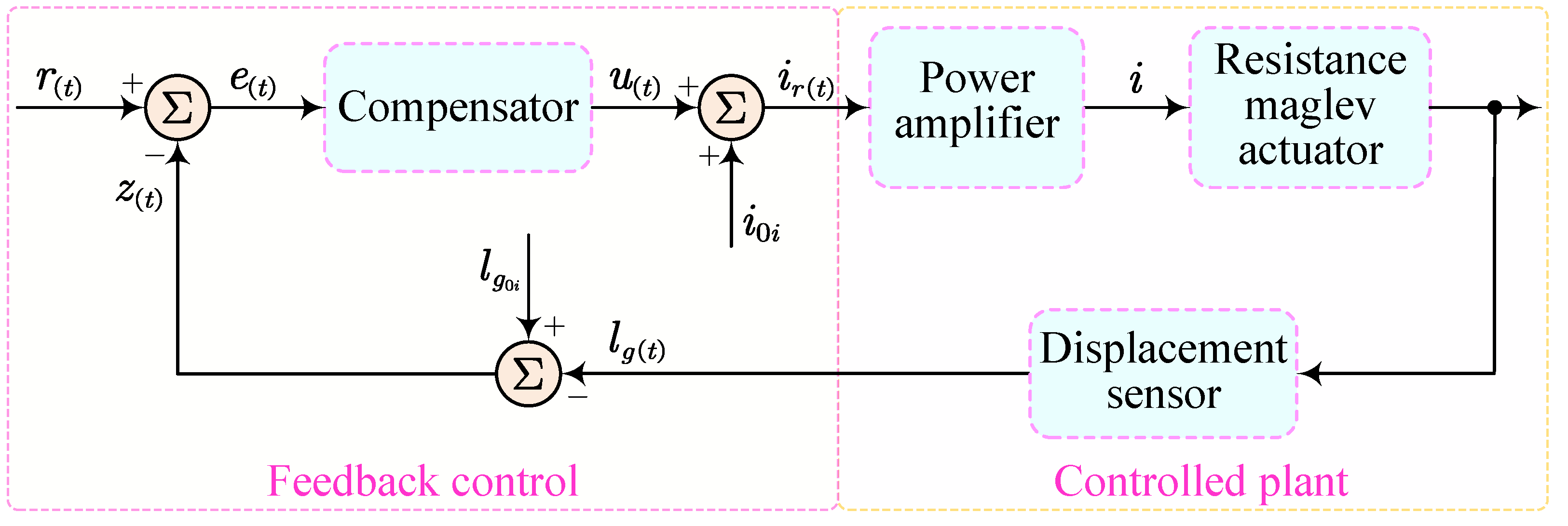
To focus on the essential control challenges, the most basic maglev system with a C-type reluctance actuator is considered for analysis. As illustrated in Figure 1, a general reluctance maglev system is composed of four main units: a reluctance actuator, a power amplifier unit, a levitation controller and a displacement sensor. Due to its inherent open-loop instability, closed-loop control is indispensable for stable operation. The displacement sensor provides real-time feedback with high resolution, while the levitation controller executes a control algorithm to generate control outputs that track the reference command. As a typical power electronic subsystem, the power amplifier implements closed-loop current control via chopper modulation. Finally, under current excitation, magnetic flux is generated in the ferromagnetic structure of the reluctance actuator, resulting in a reluctance force that compensates for gravity and disturbances. Besides the hardware components, the feedback control algorithm is a core element of the maglev system and largely dictates its performance.

2.2. Magnetic Modeling

To clarify the characteristics of the C-type reluctance actuator, magnetic flux path analysis is adopted for reluctance force modeling. The modeling originates from two fundamental magnetostatic equations in integral form: the Ampère–Maxwell law and Gauss’s law for magnetism, as shown in Equations (1) and (2). Moreover, Equations (3) and (4) describe the basic relationships between magnetic flux, magnetic flux density, and magnetic field intensity.
C H · d l = Γ J · d s
S B · d s = 0
Φ = D B · d s
B = μ 0 H + M = μ r · μ 0 · H
where C denotes a generic closed contour and H represents magnetic field intensity. J is the electric current density passing through the surface Γ , which is bounded by the contour C. S denotes a generic closed surface, and D represents a generic open surface. B represents magnetic flux density, and Φ is the magnetic flux. Then, μ 0 is the vacuum permeability, M is the magnetic susceptibility, and μ r denotes relative permeability.
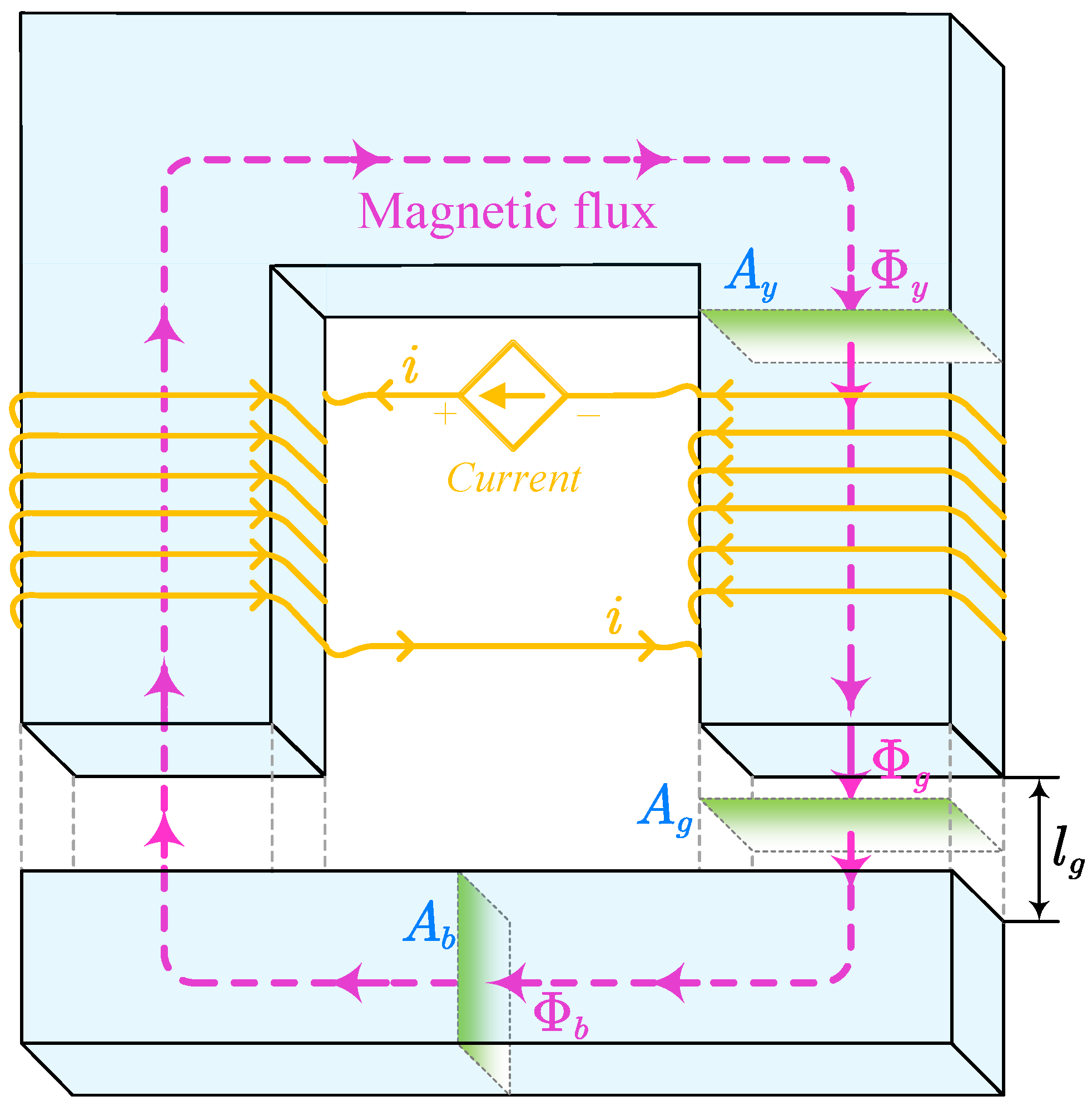
Assuming that magnetic leakage is negligible, the main flux path of the C-type reluctance actuator is illustrated in Figure 2. Considering a simplified model, the flux path loop is divided into four segments based on permeability: the ferromagnetic yoke, a pair of air gaps, and the levitated body. Afterwards, referring to Equation (1), the relationship between the segmented H field and the current source from the coil can be described as Equation (5). Similarly, by applying Equation (2) to the interfaces between segments, it follows that the magnetic flux remains continuous across all components as shown in Equation (6). Solving Equations (3)–(6) gives the magnetic flux density of the air gaps, as expressed in Equation (7).
H y l y + 2 H g l g + H b l b = n i
Φ y = Φ g = Φ b
B g = μ 0 n i A g l y A c μ r y + 2 l g + A g l b A b μ r b
in these expressions, n is the total number of coil turns on the yokes, and i is the excitation current. H y , H g , and H b represent the magnetic field intensities of the yokes, air gaps, and levitated body, respectively. Similarly, l y , l g , and l b denote the lengths of the path, and Φ y , Φ g and Φ b denote the magnetic fluxes in the these segments, respectively. Also, A y , A g and A b indicate the cross-sectional area in each segment, respectively. The μ r y is the relative permeability of the yokes, and the μ r b is that of the levitated body.
Generally, the yokes and the levitated body are manufactured from soft magnetic materials, which exhibit high initial magnetic susceptibility M. Therefore, under conditions below flux saturation, their relative permeability μ r y and μ r b can reach up to 10 4 10 5 . Thus, the minor terms in Equation (7) can be neglected, yielding the simplified form in Equation (8). Accordingly, the total magnetic energy stored in the pair of air gaps is formulated in Equation (9). Afterwards, based on the virtual work principle, the reluctance force acting between the yokes and the levitated body is derived from the partial derivative of the total magnetic energy with respect to the air-gap length, as shown in Equation (10).
B g = μ 0 n i 2 l g
W m = 1 2 B g H g V g = B g 2 A g l g μ 0
F m = W m l g = B g 2 A g μ 0 = μ 0 n 2 A g 4 · i 2 l g 2
here, W m corresponds to its total magnetic energy, V g is the total volume of the pair of air gaps, l g is the air-gap length, and F m denotes the reluctance force.

2.3. Dynamic Analysis and Modeling

The reluctance maglev system introduced in Section 2.1 and Section 2.2 is employed to perform motion control in the vertical direction. Defining vertically upward as a positive displacement axis, the dynamic equilibrium of the levitated body can be described by the second-order differential equation, as shown in Equation (11). As Equation (10) indicates, the reluctance force introduces strong intrinsic nonlinearity into this dynamic system. Consequently, a linearization process is necessary to facilitate control system design and analysis with linear control theory. The linear approximation is carried out around the equilibrium operating point defined with Equation (12), at which the reluctance force equals the gravity. By performing a Taylor series expansion on Equation (10) and neglecting the higher-order minor terms, the linearized reluctance force is expressed in Equation (13).
m z ¨ = F m m g c z ˙
F m i 0 , l g 0 m g = 0
F m F m i 0 , l g 0 = F m i i i 0 + F m l g l g l g 0
where m is the mass of the levitated body and g is the gravitational acceleration. z denotes the displacement in the vertical direction, which can be given as z = l g 0 l g . c represents the damping coefficient, which is generally ignored in maglev systems operating in air or vacuum. i 0 and l g 0 indicate the offset current and the steady-state air-gap length at the operating point, respectively. l g 0 and i 0 are the air-gap length and excitation current of equilibrium operating point respectively.
The linearized differential equation, as presented in Equation (14), is obtained by solving Equations (11)–(13) with the damping term omitted. In this linearized dynamic model, the control current i c serves as the input and the displacement of levitated body z as the output. Then, the transfer function in Equation (15) is obtained by applying the Laplace transform.
m z ¨ = k s i i c + k s z z
G s = Z s I c s = k s i m s 2 k s z
k s i = F m i = μ 0 n 2 A g 2 · i 0 l g 0 2 = m g · μ 0 n 2 A g l g 0
k s z = F m l g = μ 0 n 2 A g 2 · i 0 2 l g 0 3 = 2 m g l g 0
in the above equations, i c is the control current, which is given as i c = i i 0 . k s i and k s z denote the current stiffness coefficient and the air-gap stiffness coefficient, respectively.

3. Control System Analysis

3.1. Basic Feedback Configuration

As indicated in Equation (18), the transfer function of the reluctance maglev system contains a pair of poles positioned along the real axis in the s-domain. One of the poles lies in the right-half plane (RHP), leading to open-loop instability. Physically, the inherent instability is attributed to the natural negative stiffness k s z of the air gap. Specifically, when the air-gap length decreases below its target value, the reluctance force increases instead of weakening, which opposes the restoring tendency and leads to further reduction of the gap. Hence, the basic feedback configuration illustrated in Figure 3 is essential to introduce positive stiffness and stabilize the dynamic system. In this configuration, a certain equilibrium operating point of the reluctance maglev system is set as the initial air-gap length l g 0 i and the offset current i 0 i , while a linear compensator is utilized to tune system performance.
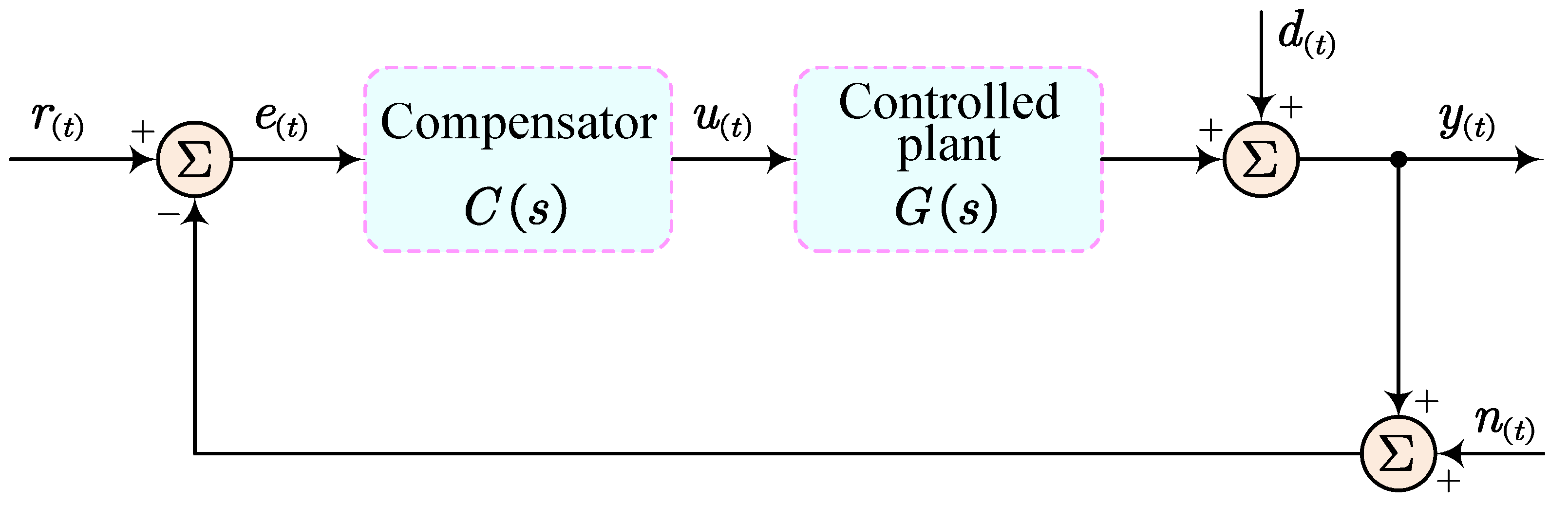
For the purpose of control system analysis, a linearized feedback model with a given operating point is outlined in Figure 4. Here, the proportional-derivative (PD) compensator, as defined in Equation (19), is first used to analyze the system, and the resulting open-loop transfer function L s is given in Equation (20). Then, the closed-loop transfer function T s of feedback system can be derived as shown in Equation (21), while the transfer paths from reference r ( t ) and noise n ( t ) to output y ( t ) are expressed in Equation (22). Accordingly, a well-compensated closed-loop maglev system is expected to demonstrate low-pass behavior: ensuring precise reference tracking in the low-frequency range and suppressing high-frequency noise. Furthermore, the sensitivity transfer function S s , as formulated in Equation (23) and Equation (24), quantifies the impact of system uncertainties and external disturbances d ( t ) on the output. The sensitivity function generally features high-pass behavior, effectively suppressing disturbances and parameter perturbation in low-frequency to ensure system robustness. In fact, the sensitivity transfer function is defined as the ratio of the closed-loop output to the open-loop output, reflecting how feedback influences the system response.
p G 1 , p G 2 = ± k s z m
C s = k P + k D s
L s = C s G s = k s i k P + k D s m s 2 k s z
T s = L s 1 + L s = k s i k P + k D s m s 2 + k s i k D s + k s i k P k s z
T s = Y s R s = Y s N s
S s = 1 1 + L s = m s 2 k s z m s 2 + k s i k D s + k s i k P k s z
S s = d T s / T s d G s / G s = Y s D s
where p G 1 , p G 2 are the two poles of the transfer function G ( s ) . k P represents the proportional gain of the PD compensator and k D denotes the derivative gain.

3.2. Dynamic Characteristics Analysis

From an intuitive physical perspective, a reluctance maglev system with well-compensated feedback is capable of restoring the air gap and damping its oscillations. It can be considered equivalent to a standard mass-spring-damper system, whose characteristic equation D ( s ) from the closed-loop transfer function T ( s ) is defined in Equation (25). Hence, the natural frequency and damping ratio of the equivalent system can be derived, as shown in Equations (26) and (27). In addition, these parameters are defined in terms of the equivalent stiffness and damping coefficients, which are also explicitly expressed in two equations. Therefore, based on Equations (26) and (27), the equivalent stiffness and damping coefficients of the system can be obtained, as shown in Equations (28) and (29).
D s = m s 2 + k s i k D s + k s i k P k s z = s 2 + 2 ζ ω n s + ω n 2
ω n = k s i k P k s z m = k s e m
ζ = k s i k D 2 m k s i k P k s z = c e 2 m k s e
k s e = k s i k P k s z
c e = k s i k D
in the expressions, ω n is the natural frequency, and ζ is the damping ratio of equivalent system. k s e and c e denote equivalent stiffness and damping coefficients, respectively.
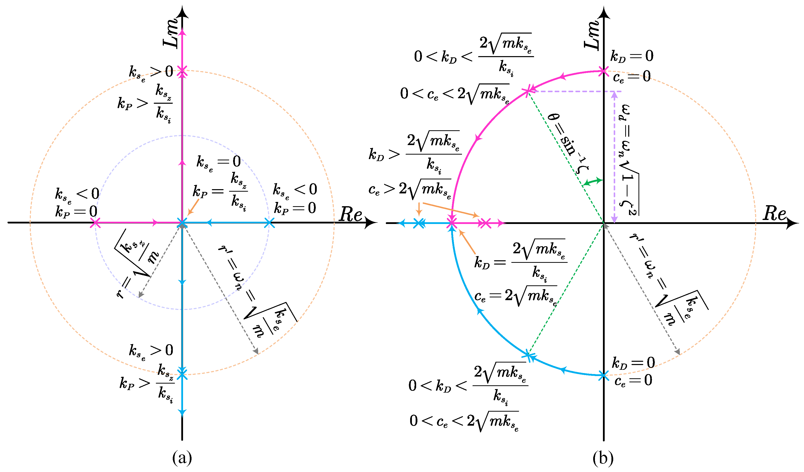
To analyze the dynamic characteristics of the system, the root locus method is utilized. By solving the characteristic equation D ( s ) given in Equation (25), the coordinates of the closed-loop poles in the s-domain can be determined as expressed in Equation (30). As illustrated in Figure 5a, the effect of the proportional gain in the PD compensator is first analyzed. In this process, the derivative gain k D is held constant at zero, and the proportional gain k P is increased from zero. Initially, with k P = 0 , the pair of poles is located on the real axis, resulting from the naturally negative stiffness of the air gap. Then, as the k P increases within the range 0 < k P < k s z / k s i , the negative stiffness is partially compensated by feedback. However, the equivalent stiffness remains negative, and the presence of an RHP pole still renders the system unstable. When k P = k s z / k s i , the two poles coincide at the origin of the s-domain, and the system enters a marginally stable state. In this condition, the air gap exhibits zero equivalent stiffness, resulting in neither convergence nor divergence. Afterwards, as k P exceeds k s z / k s i , the two poles form a conjugate pair on the imaginary axis, and the system remains marginally stable. Physically, it behaves like an ideal spring with positive equivalent stiffness, oscillating at its natural frequency ω n .
The effect of the derivative gain k D on dynamic characteristics is illustrated in Figure 5b, following the establishment of positive equivalent stiffness via proportional control. It is evident that both poles move into the left-half plane (LHP) of the s-domain as long as k D > 0 . In addition, when k D = 2 m k s e / k s i , the system exhibits critical damping with a damping ratio of ζ = 1 . For values of k D below or above this threshold, the system is underdamped or overdamped, respectively. However, in reluctance maglev systems, excessive derivative gain degrades robustness due to the high sensitivity of pure derivative operation to sensor noise. Consequently, critically damped and overdamped designs are rarely feasible in control engineering. In summary, the stability condition that ensures both poles reside in the LHP is expressed in Equation (31), and it can be further supported by the Routh–Hurwitz criterion. From a mechanically meaningful perspective, this condition can be interpreted as requiring both positive equivalent stiffness k s e and positive equivalent damping c e .
p T 1 , p T 2 = k s i k D 2 m ± k s i 2 k D 2 4 m 2 k s i k P k s z m
k P > k s z / k s i k D > 0 k s z > 0 c e > 0
here, p T 1 and p T 2 are the two poles of the closed-loop transfer function T ( s ) .

3.3. Nonlinear Effects with Air Gap Variation

As described in Section 2.3, the reluctance maglev system exhibits inherent nonlinearity with respect to the air-gap length and excitation current. Accordingly, it is necessary to evaluate the impact of this nonlinearity on system stability and performance under different equilibrium operating points. By combining Equations (16) and (17), Equation (32) can be obtained, which provides the stable lower threshold of proportional gain k P under different operating conditions. It indicates that the critical value of k P for achieving positive equivalent stiffness depends solely on the mass of levitated body and is independent of the air-gap length. In most practical scenarios, the levitated mass in reluctance maglev servo systems is typically treated as a constant parameter. Hence, the minimum k P required for stable levitation can be directly derived from the geometry and parameters of the reluctance actuator.
k P > k s i k s z = i 0 l g 0 = 4 m g μ 0 n 2 A g
k s e = μ 0 n 2 A g · m g l g 0 k P 4 m g μ 0 n 2 A g
c e = μ 0 n 2 A g · m g l g 0 · k D
ζ = 1 l g 0 k D 2 · μ 0 n 2 A g · m g 4 m · k P · μ 0 n 2 A g · m g 2 m g 1 2
As for the equivalent stiffness k s e and equivalent damping c e , Equations (28) and (29) are respectively solved in combination with Equations (12), (16), and (17), yielding the results shown in Equations (33) and (34). It can be observed that, with constant PD gains and levitated mass, both the equivalent stiffness and damping decrease with increasing operating air-gap length l g 0 , following an inverse proportionality. Furthermore, the damping ratio ζ decreases as the l g 0 increases, following an inverse square-root relationship, as indicated in Equation (35). Consequently, in the s-domain, the two open-loop poles on the real axis move progressively closer to the origin as l g 0 increases. Simultaneously, the corresponding closed-loop conjugate poles in the left-half plane exhibit a reduced modulus r and a smaller argument θ , which are illustrated in Figure 5b. The shift in pole locations directly affects the control system performance, which manifests in the time domain as increased settling time and overshoot. Similarly, the system exhibits reduced disturbance rejection capability, with larger air-gap variations and slower convergence. In practical terms, the nonlinear effects of the reluctance actuator result in significantly varying dynamic responses during long-stroke operation, making it difficult to achieve satisfactory performance in both maximum and minimum air-gap conditions.

3.4. Robustness Constraints

In Section 3.2 and Section 3.3, the control system dynamic characteristics of the reluctance maglev system are analyzed. Analysis in the s-domain suggests that long-stroke stability could be obtained by increasing the PD gains to sufficiently high levels. Nevertheless, in engineering practice, this approach is not feasible: the PD gains cannot be increased indefinitely, nor can the levitation air gap be reduced arbitrarily, mainly due to robustness constraints of the control system. In practice, achieving proper tuning becomes increasingly difficult as the stable air gap decreases. From an intuitive physical perspective, a smaller air gap corresponds to a higher inherent negative stiffness, thereby intensifying the natural instability of the control system. From a control theory perspective, the Bode integral theorem captures and quantifies the challenge of designing stable control systems, and provides an elegant explanation for this phenomenon. As shown in Equation (36), the frequency-domain integral of the sensitivity transfer function S ( s ) equals zero. This implies that suppressing sensitivity in one frequency range will inevitably lead to an increase in another, a phenomenon also known as the “waterbed effect.” It follows that feedback control cannot improve the suppression capability of disturbance and perturbation in one frequency range without inevitably worsening it in another. In fact, for open-loop unstable systems such as the reluctance maglev system, the integral of the sensitivity depends on the RHP unstable poles, as shown in Equation (37). As a result, the loop shaping attainable via feedback control is more strictly constrained, and achieving a low sensitivity through simple parameter tuning becomes even more challenging. In addition, Equation (38) is derived by substituting Equations (12) and (17) into Equation (18). It indicates that the open-loop poles of the reluctance maglev system depend solely on the operating air-gap length, and are inversely proportional to its square root. This exhibits the same characteristic as the inverted pendulum system, which is a well-known typical plant in control theory.
0 ln S j ω d ω = 0
0 ln S j ω d ω = π Re p k
p G 1 , p G 2 = ± μ 0 n 2 A g 2 m · i 0 2 l g 0 3 = ± 2 g l g 0
where j is the imaginary unit and ω is frequency. The p k denotes unstable poles in RHP.
By introducing the concept of available bandwidth, Gunter Stein developed a methodology for quantifying the inherent instability of the inverted pendulum system and an aircraft control system [31]. It also can provide valuable insights into the inherent constraints in the design of reluctance maglev control systems. With the concept of available bandwidth, the Bode integral is reformulated into the finite integral expressions. As shown in Equations (39) and (40), the improvement or degradation of sensitivity occurs almost entirely within the available bandwidth, while the sensitivity integral outside this range contributes only a negligible error. It is critical to note that the available bandwidth is not defined by the open-loop crossover frequency or the closed-loop −3 dB point, but is instead independent of the feedback design process and is imposed as an a priori constraint by the physical hardware in the control loop. As shown in Figure 1, each subsystem unit can preserve frequency response fidelity only within an inherently finite bandwidth. The smallest of these bandwidths, which serves as the “bottleneck,” defines the available bandwidth of the whole system. For the levitation controller, the finite bandwidth is limited by the computational capability of the embedded system. According to the Nyquist–Shannon sampling theorem, the sampling/command cycle frequency is exceed twice the theoretical maximum frequency of the analog signals that can be captured or generated. In engineering practice, its finite bandwidth is typically defined as 5–10 times smaller than the sampling/command cycle frequency to account for noise impacts. This is also why advanced algorithms rarely succeed in standard embedded systems, where high computational cost constrains high-frequency response and robustness. For the power amplifier and displacement sensor, the finite bandwidth is generally limited by their −3 dB frequency. As for the reluctance maglev actuator, its constraints mainly come from mechanical resonance; therefore, high structural stiffness is typically adopted in design.
0 Ω a ln S j ω d ω = δ
0 Ω a ln S j ω d ω = π Re p k + δ
in the equations, the Ω a indicates the available bandwidth, and the δ shows a negligible small error.
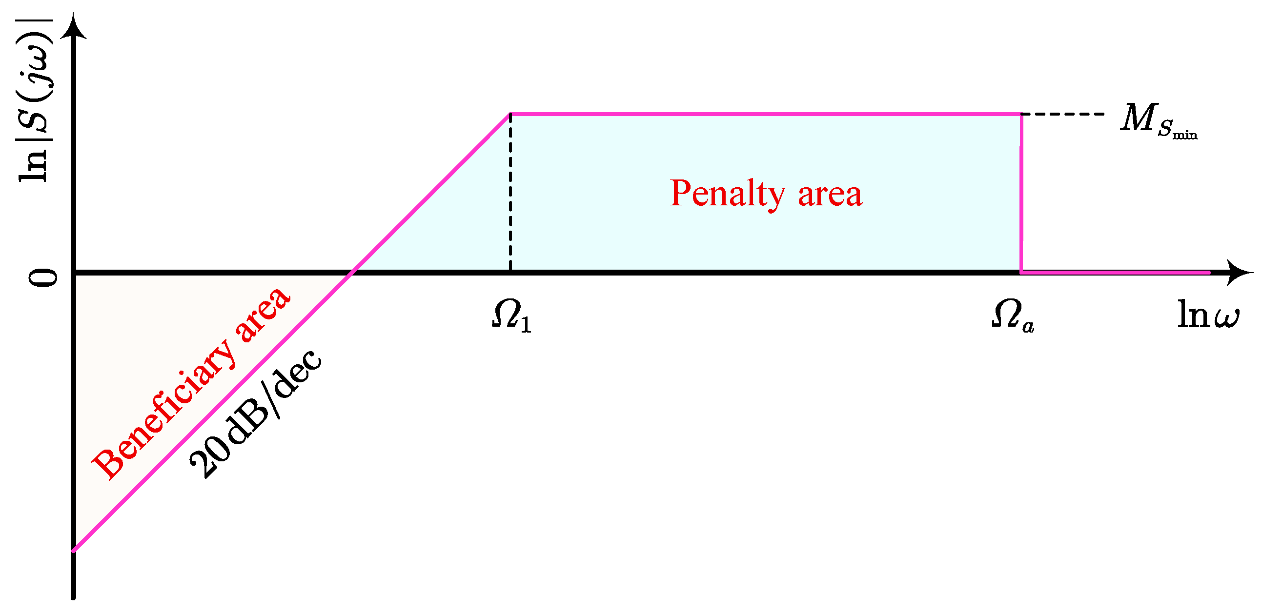
For a reluctance maglev system with given hardware components, Equation (40) provides a quantitative framework for assessing robust stability. The sensitivity transfer function S ( s ) exhibits a high-pass behavior, featuring low sensitivity in the low-frequency range, which then rises and levels off as the frequency increases. For quantitative calculation, the ideal sensitivity profile in the frequency domain is presented in Figure 6. It is assumed that the sensitivity rises from the zero frequency with a slope of 20 dB/dec, remains constant after reaching its peak at the corner frequency, and then sharply decays to unity beyond the available bandwidth. It is worth noting that this profile is not feasible in engineering practice, it merely defines the theoretical minimum of sensitivity peak. By substituting the piecewise function of the profile into Equation (40), Equation (41) the can be obtained. Then, by performing integration by parts on this equation and combining it with Equation (38), the minimum sensitivity peak is obtained as expressed in Equation (42). Furthermore, the sensitivity peak also serves as a measure of system robustness, and as shown in Equation (43), it is the reciprocal of the vector margin, which is defined as the shortest distance from the Nyquist plot to the critical point 1 , j 0 . Although the vector margin is a more precise and compact measure of robustness, the gain margin and the phase margin remain widely used in engineering practice. Their relationships with the sensitivity peak are given in Equation (44). They indicate that reducing the sensitivity peak increases the stability margin, and thereby enhances system robustness.
0 Ω 1 ln ω M S min Ω 1 d ω + Ω a Ω 1 · ln M S min = π · Re p G 1
M S min = exp π · 2 g l g 0 + Ω 1 / Ω a
V M = 1 M S
G M 20 lg M S M S 1 P M 2 sin 1 1 2 M S 1 M S
in the above expressions, M S represents the sensitivity peak and M S min denotes the theoretical minimum of sensitivity peak. Ω 1 indicates the corner frequency, which also denotes the desired performance bandwidth. V M , P M and G M are vector margin, gain margin, and phase margin, respectively.
Therefore, for a given control loop configuration and stability margin requirement, the theoretical lower air-gap length can be calculated and is determined by the desired performance bandwidth. Furthermore, for a certain operating point, a higher desired performance bandwidth contributes to reducing the low-frequency gain attenuation of compensation sensitivity transfer function T ( s ) , resulting in better closed-loop tracking performance. Nevertheless, it also inevitably leads to a higher theoretical minimum sensitivity peak, which degrades the potential of robustness. This suggests that, in long-stroke reluctance maglev systems, using a large constant proportional gain k P to achieve acceptable equivalent stiffness at large air gaps is impractical, because it can severely compromise robustness when operating at small air gaps. On the one hand, a higher proportional gain increases the equivalent stiffness but also broadens the desired performance bandwidth. On the other hand, as indicated in Equation (42), a smaller air gap causes a larger real part of the unstable pole, which further worsens the level of sensitivity peak. Consequently, for long-stroke reluctance maglev systems, it is beneficial to adopt an gain scheduling strategy to ensure robustness at small operating air gaps while simultaneously enhancing response performance at large air gaps.

4. Control Strategy Design

4.1. Feedforward Compensation

In the steady-state, the relationship between the air-gap ength and the excitation current of the reluctance maglev system can be derived as Equation (45) by simultaneously solving Equations (10) and (11) while neglecting the derivative term. It indicates that, under a constant levitated mass, the steady-state current exhibits a linear relationship with the steady-state air-gap length. In addition, the basic feedback configuration shown in Figure 3 is formulated as Equation (46), in which the PD compensator defined by Equation (19) is used. Then, solving Equations (45) and (46) while disregarding the derivative term, the steady-state equation under the basic feedback configuration can be built as Equation (47). Subsequently, substituting the equilibrium operating point Equation (12), which defines the initial air gap and the offset current, yields the steady-state error expressions as Equation (48). It demonstrates that the steady-state error increases linearly with the reference input. This phenomenon can be explained by Equation (49), which shows that the variation in excitation current required for steady-state displacement is compensated by the steady-state error and the proportional gain.
i s = 4 m g μ 0 n 2 A g · l g s
e t = r t z t z t = l g 0 i l g t i t = k P · e t + k D · e ˙ t + i 0 i
k P · e t s + i 0 i = 4 m g μ 0 n 2 A g · l g 0 i z t s
r t e t s = 1 k P · μ 0 n 2 A g 4 m g
i s i 0 i = k P · e t s = 4 m g μ 0 n 2 A g · z t s
where i 0 i , i t and i s represent offset current, real excitation current and steady-state current, respectively. l g 0 i , the l g t and the l g s denote initial air-gap length, real air-gap length and steady-state air-gap length, respectively. r t is reference input, z t is real displacement, and z t s is steady-state displacement. e t is real error and e t s is steady-state error.
For the long-stroke reluctance maglev systems, the air-gap length is variable during operation to enable positioning control, which inherently requires a variable reference input. In such application scenarios, a predictable steady-state error inevitably appears; as previously discussed, the PD-based basic feedback configuration is inadequate for positioning control. Consequently, the real-time compensation must be incorporated into the feedback configuration instead of relying on a pair of the initial air gap and constant offset current. In practice, two underlying approaches are widely adopted: integral compensation and feedforward compensation. In essence, the reference input shifts the operating air-gap length while the compensator biases the offset current, as shown in Equation (50), thereby redefining a new equilibrium operating point which is explored in Section 3.3. The integral compensation is commonly integrated into the feedback loop to constitute a PID compensator, as expressed in Equation (51). From a frequency-domain perspective, the integrator exhibits infinite DC gain ( ω = 0 ), thereby completely eliminating steady-state error. Nevertheless, its drawback is that it introduces significant phase lag at frequencies below its corner frequency ( ω = 1 / T 1 = k I / k P ), thereby decreasing phase margin. For levitation control, a small integral gain can mitigate the impact of phase lag on robustness, but it leads to a longer settling time. Especially in long-stroke operation, achieving an acceptable compromise between robustness and tracking performance is notably challenging.
As for the feedforward compensation approach, a real-time offset computed from the reference signal is injected directly to the output of feedback loop. Following the steady-state linear relation in Equation (45), the feedforward law for the reluctance maglev system can be presented as Equation (52). As it relies solely on three structural parameters of the reluctance actuator, its implementation is independent of operator skill. With a feedforward compensator, the theoretically predictable steady-state error can be eliminated. However, residual steady-state error remains under modeling inaccuracies and external disturbances, which is a key drawback of this approach. Accordingly, in long-stroke reluctance maglev systems prioritizing positioning accuracy, the integral and feedforward compensators should be employed in parallel. The integral gain can be set sufficiently small so that the corner frequency of PID is well below the crossover frequency of the system, thereby preserving phase margin and overall robustness. In scenarios that prioritize dynamic response and robustness, such as when the reluctance maglev serves as the inner loop subsystem within a overall control architecture, a feedforward-only strategy is preferable.
l g 0 = l g 0 i z t s i 0 = i 0 i + i f c t e t s = r t z t s = 0
i t = k P · e t + k I 0 t e τ · d τ + k D · e ˙ t + i 0 i
i f c t = k f · r t = 4 m g μ 0 n 2 A g · λ c · r t
in these expressions, k I is the integral gain of the PID compensator. i f c t denotes the feedforward compensation current and k f represents the feedforward compensation coefficient. λ c indicates the feedforward calibration factor, which is used to manually correct modeling inaccuracies in tuning.

4.2. Gain Scheduling PD Compensator

As discussed in Section 3.3, with a constant-gains PD compensator, the reluctance maglev control system exhibits marked air-gap length dependence: equivalent stiffness, equivalent damping, and the damping ratio all vary with the operating air-gap length, so the system cannot maintain uniform, satisfactory dynamic response over the long stroke. As also noted in Section 3.4, robustness constraints impose a design trade-off between the stability margin at small air gaps and the control performance at large air gaps. Since operation at small air gaps inherently restricts the attainable stability margin, the constant gains tuned to satisfy large-gap response inevitably further degrades small-gap robustness. To overcome the above shortcomings, a PD-based gain scheduling algorithm is proposed to maintain constant equivalent stiffness and damping across the operating stroke.
Firstly, the stiffness ratio ε is defined in Equation (53) to express the desired equivalent stiffness as a multiple of the natural negative air-gap stiffness evaluated at the initial air gap. By combining Equations (17), (33), (50) and (53), the constant equivalent stiffness equation with adaptable proportional gain is expressed as Equation (54), which indicates that the equivalent stiffness remains at the target value after shifting to a new equilibrium operating point. Then, the adaptable proportional gain k P A follows from solving this equation and is given in Equation (55), which consists of an initial term and an incremental term. As shown in Equation (56), the initial term denotes the proportional gain that sets the equivalent stiffness to a target value at the initial operating air gap. The incremental term in Equation (57) denotes the scheduling proportional-gain increment needed to keep the equivalent stiffness constant as the operating air gap changes.
k s e d = ε · k s z i
μ 0 n 2 A g · m g l g 0 i r t k P A 4 m g μ 0 n 2 A g = ε · 2 m g l g 0 i
k P A = k P i + Δ k P
k P i = 2 ε + 1 · m g μ 0 n 2 A g
Δ k P = 2 ε l g 0 i · m g μ 0 n 2 A g · r t
among them, the k s e d is the desired equivalent stiffness, the ε is the stiffness ratio, and the k s z i is the air gap stiffness at initial operating air-gap length. The k P A indicates the adaptable proportional gain, the k P i denotes the initial proportional gain, and the Δ k P means the scheduling increment of proportional gain.
Subsequently, by combining the Equations (27) and (53), the desired equivalent damping is defined with the damping ratio and the desired equivalent stiffness as shown in Equation (58). Substituting Equations (17), (34) and (50) into this expression yields the constant equivalent damping relation as Equation (59), which denotes that the equivalent damping and damping ratio can be maintained using an adaptable derivative gain. The solutions of the adaptable derivative gain are shown in Equation (60), which can also be expressed as the sum of the initial value and the increment. The initial value in Equation (61) corresponds to the derivative gain at the initial operating air gap, while the scheduling increment of derivative gain in Equation (62) quantifies the compensation required for varying reference inputs.
c e d = 2 ζ · m k s e d = 2 ζ · m ε k s z i = k s i k D A
2 ζ · 2 ε m 2 g l g 0 i = m g μ 0 n 2 A g l g 0 i r t · k D A
k D A = k D i + Δ k D
k D i = 2 ζ · 2 m ε l g 0 i μ 0 n 2 A g
Δ k D = 2 ζ · 2 m ε l g 0 i μ 0 n 2 A g · r t
where c e d is the desired equivalent damping. k D A denotes the adaptable derivative gain, k D i indicates the initial derivative gain, and Δ k D represents the scheduling increment of derivative gain.
From an intuitive physical perspective, the two scheduling PD gains enforce constant equivalent stiffness and damping at steady-state at each position of the reluctance maglev system across the entire stroke. From the perspective of control theory, this is essentially a pole-placement approach. With the equivalent stiffness and damping held constant, the two closed-loop poles are fixed at the LHP of s-domain coordinates given in Equation (63). Hence, the control system remains closed-loop stable throughout the PD gain scheduling process. Meanwhile, since the closed-loop zero is well separated from the dominant pole, its transient decay is much smaller than that of closed-loop dynamics, rendering its effect on the response of the time and frequency domains negligible. As a result, this PD-based gain scheduling algorithm delivers uniform performance over the full stroke. Moreover, for general reluctance maglev systems operating at a constant air-gap length, the initial-gain expressions given in Equations (56) and (61) are also suitable for determining the PD gains. It is noteworthy that the algorithm relies solely on basic parameters, and the appropriate compensator gains can be determined with only simple calculations. Therefore, for most reluctance maglev systems, including magnetic bearings, it is independent of operator expertise for gain tuning.
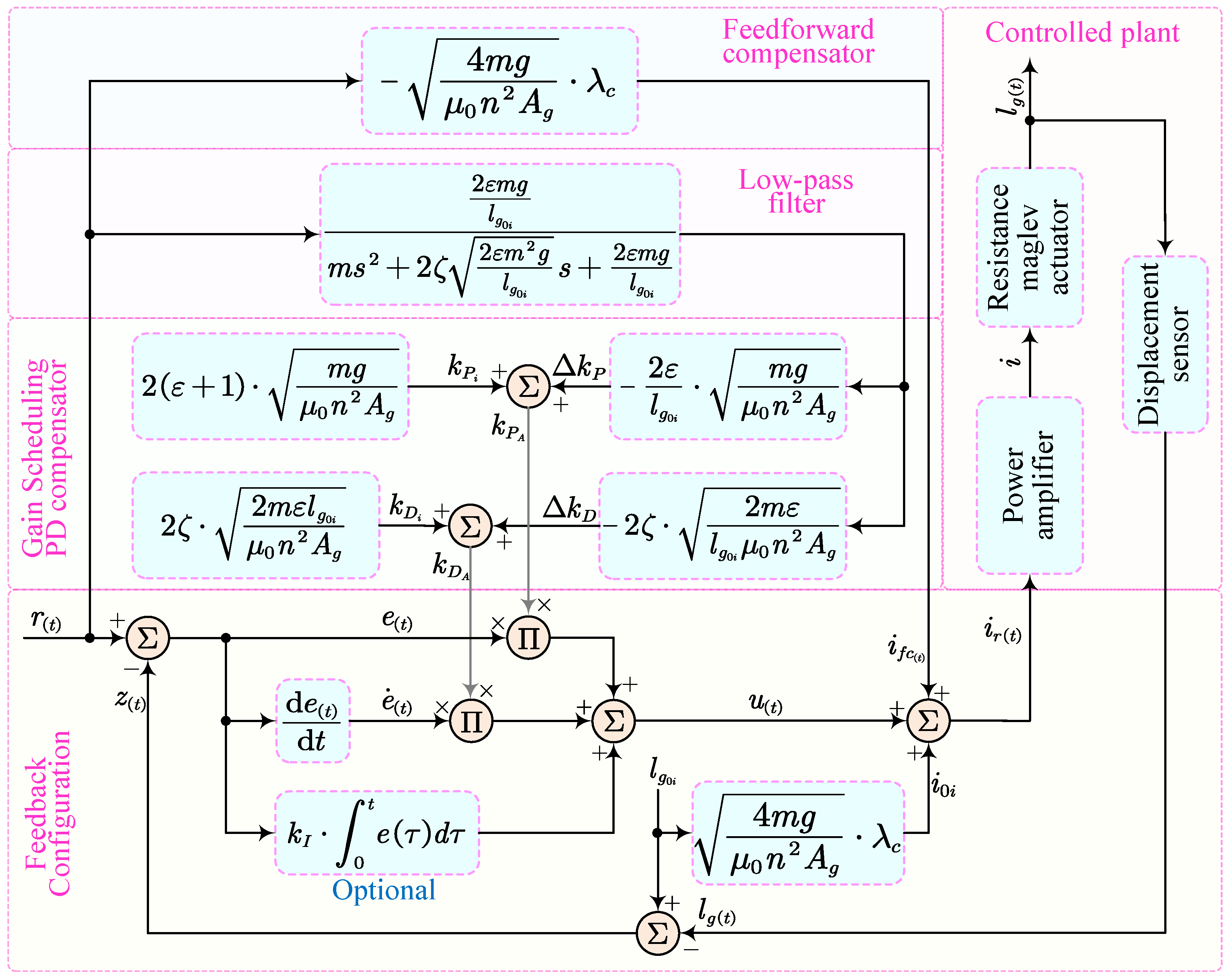
Nevertheless, the above approach has the drawback that abrupt changes in the reference input, such as a step signal, induce discontinuities in PD gains. Although substituting the reference input with the measured real displacement can theoretically avoid the discontinuities, it increases the gain uncertainty and noise sensitivity of the gain scheduling PD compensator, since measurement noise cannot be entirely filtered out. Considering levitation accuracy and robustness, this substitution is not advisable. Another compromise approach involves shaping the reference input with a low-pass filter to approximate the system dynamics, and then computing the scheduling increments from the filtered signal. While this approach cannot correct deviations in the equivalent stiffness and damping caused by real displacement errors, it prevents gain discontinuities and noise worsening. Consequently, a low-pass filter with the same characteristic polynomial and pole configuration as the gain scheduling closed-loop transfer function is designed, as presented in Equation (64). In summary, the feedforward scheme is combined with the gain scheduling PD, and the resulting control strategy is shown in Figure 7.
p T 1 , p T 2 = c e d 2 m ± c e d 2 m 2 k s e d m
H s = k s e d m s 2 + c e d s + k s e d = 2 ε m g l g 0 i m s 2 + 2 ζ 2 ε m 2 g l g 0 i s + 2 ε m g l g 0 i
Figure 7. Control strategy with feedforward and gain scheduling. This strategy relies only on basic parameters of the actuator, all of which are listed in Table 1. The arrows in the diagram indicate signal flow direction.
Actuators 15 00151 g007
Table 1. Basic parameters for controller design.
ParameterSymbolValueUnit
Vacuum permeability μ 0 4 π × 10 7 N / A 2
Gravitational accelerationg9.8 m / s 2
Total coil turnsn380turns
Pole area of yoke A g 4 × 10 4 m 2
Levitated body massm0.581 kg
Stiffness ratio ε 2
Damping ratio ζ 0.707
Initial air-gap length l g 0 i 0.01 m

5. Experiments and Analysis

5.1. Prototype and Experimental System

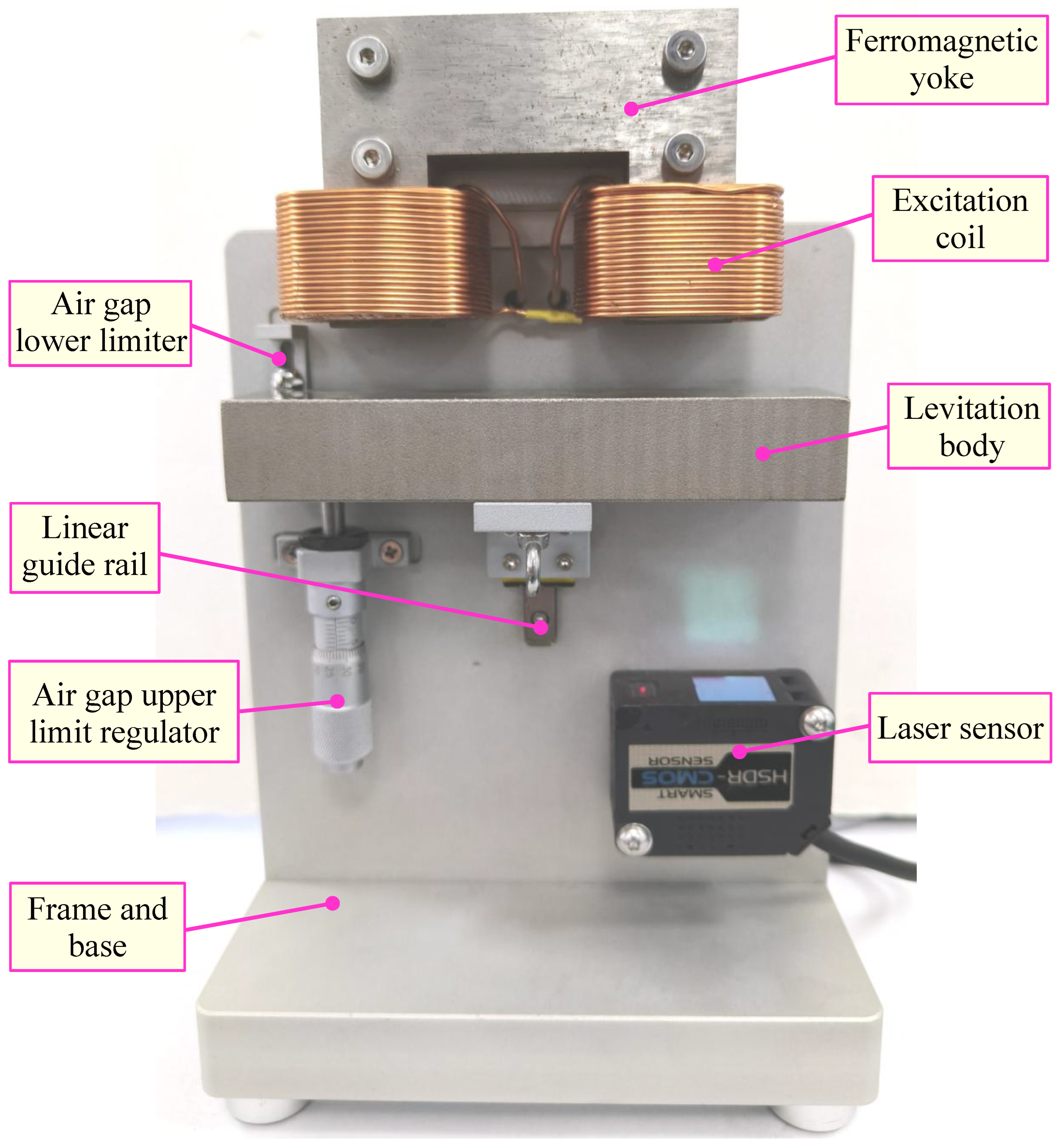
To verify the proposed control strategy and realize long-stroke stable levitation and positioning control, a prototype was constructed, as depicted in Figure 8. The core components are the C-type reluctance actuator, the levitated body, and a laser displacement sensor. The ferromagnetic yokes and the levitated body are fabricated from pure iron (DT4C), offering high initial permeability and low coercivity. The laser displacement sensor (ZX2-LD50L, OMRON Corporation, Kyoto City, Japan) features a 20 mm range, 1.5 µm resolution, and ±0.1% nonlinearity, enabling high-precision air-gap measurement. In addition, a linear guide rail is used for vertical guidance. The air-gap upper/lower limit regulators are implemented to avoid magnetic pull-in and falling, thereby defining the stroke of the levitation body. Furthermore, the control strategy described in Section 4 relies on basic parameters of the prototype, which are summarized in Table 1.
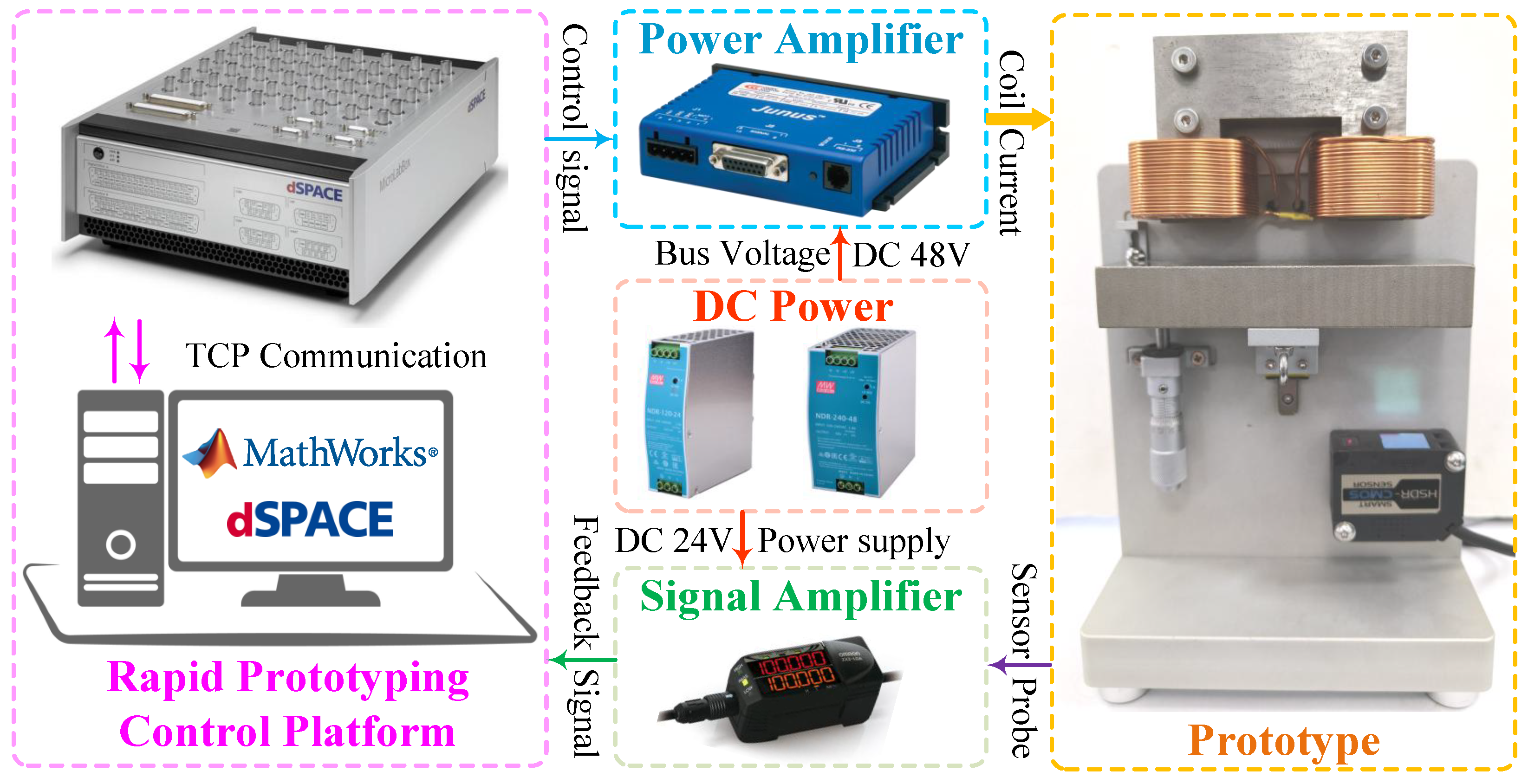
To implement feedback control, data acquisition and current excitation, the mechatronic system for experiments was built, as illustrated in Figure 9. The control program and data acquisition are implemented on a dSPACE rapid prototyping control platform (Microlabbox, dSPACE Corporation, Paderborn, Germany), which interfaces seamlessly with MATLAB/Simulink 2025b to facilitate fast algorithm development and online tuning of parameters. In this system, both air-gap feedback and control outputs are routed through the analog channels, and the sampling period is set to 10 KHz. The DC servo drive (Copley Controls JSP-180-20, Analogic Corporation, Peabody, MA, USA) is used as the power amplifier, and the bus voltage of its MOSFET H-bridge is 48 V. The internal current loop employs a PI compensator, and the resulting closed-loop bandwidth is 1 KHz. Moreover, the measurement period of laser signal amplifier (ZX2-LDA11, OMRON Corporation, Kyoto City, Japan) is configured to 60 µs.

5.2. Long-Stroke Positioning Control Experiments

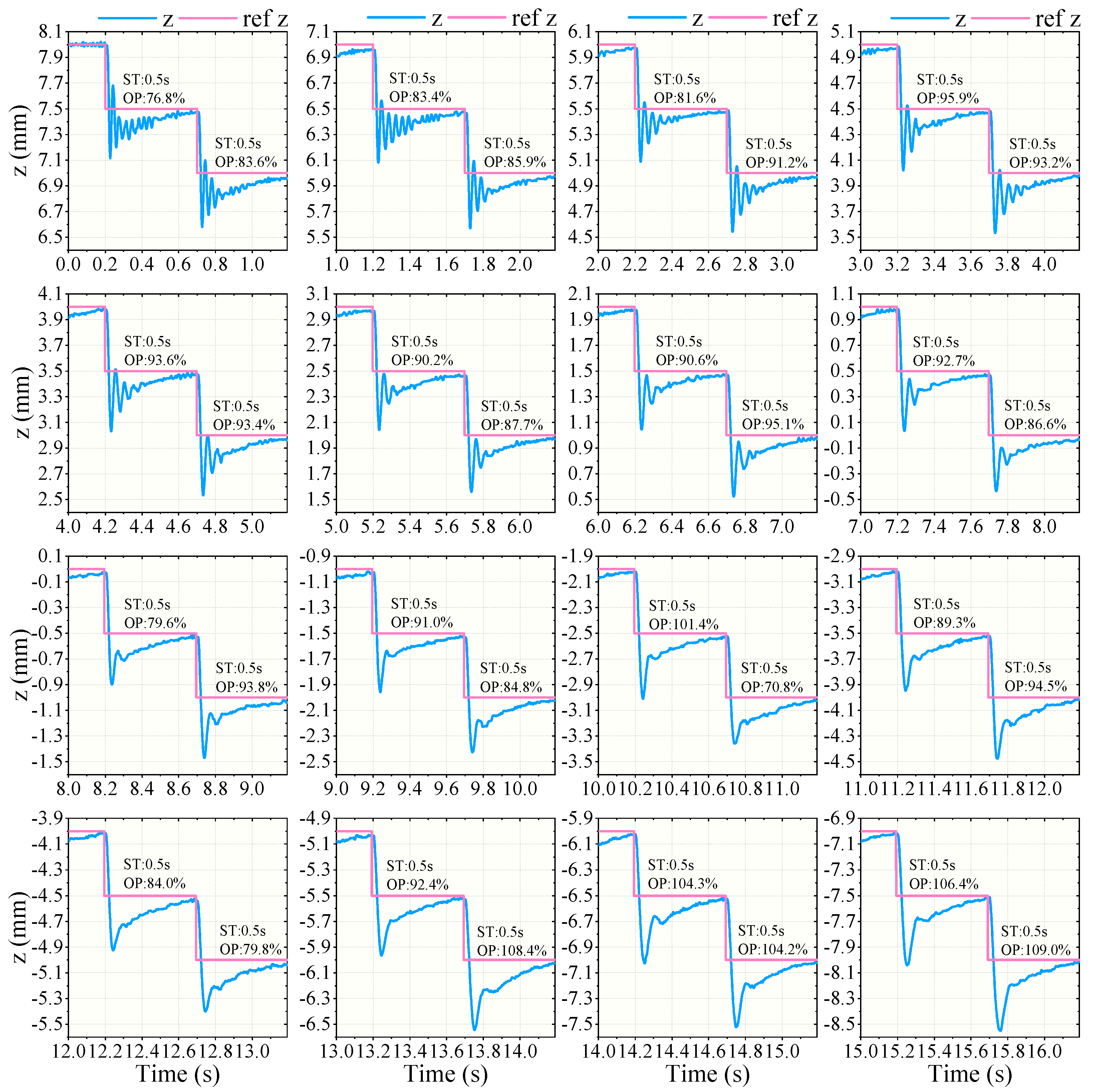
To facilitate comparison, the long-stroke positioning control experiments are first conducted with the basic feedback configuration, as depicted in Figure 3. Meanwhile, as illustrated in Equation (51), a fixed-gain PID compensator and a fixed offset current are employed to achieve closed-loop control of the levitated body displacement. As for its parameters, the calculations are based on the Table 1 values: Equations (56) and (61) determine the proportional and derivative gains, respectively, while Equation (45) is employed to obtain the offset current. To mitigate steady-state error, the integral gain is set to 10,000. Subsequently, long-stroke positioning control experiments are conducted, and the results are shown in Figure 10. The motion proceeds from +8 mm to −8 mm in vertical displacement z, with a step amplitude of 0.5 mm, yielding 32 steps to cover the entire stroke. With the initial air-gap length set to 10 mm, the air-gap length over the full stroke spans from 2 mm to 16 mm, so the maximum air-gap length is eight times the minimum.
In the results illustrated in Figure 10, two important trends emerge, both of which merit discussion. First, each step response exhibits a relatively long settling time, approximately 0.5 s. This occurs because, as discussed in Section 4.1, the steady-state current is different for each air-gap length. Based on the displacement error, the integrator compensates the control current to the steady-state current associated with the displacement setpoint. Consequently, the feedback control exhibits a gradual and slow regulation process, particularly when the integral gain is set to be small or when the step amplitude is large. Second, the step response at small air gaps exhibits pronounced oscillations, which gradually diminish as the air gap increases. The reason is that the equivalent stiffness and damping are specified at the initial air gap, and both change markedly with variations in the air gap.
Subsequently, feedforward compensation is incorporated into the basic control configuration. By injecting the known steady-state relationship into the control input, satisfactory steady-state accuracy and settling time can be attained with a much smaller integral gain. Accordingly, it is reduced to 1000, which is one tenth of that in the previous experiment. Step experiments over air-gap lengths from 2 mm to 16 mm are conducted again, and the results are shown in Figure 11. With real-time feedforward compensation of the offset current from the reference input, the settling time is markedly shortened, and the steady-state error is eliminated in approximately 0.2 s. However, pronounced oscillations are still observed at small air gaps, and they diminish with increasing air-gap length, accompanied by a gradual reduction in overshoot. This indicates that feedforward compensation can effectively alleviate the burden of the integrator in long-stroke positioning control of the reluctance maglev system, but it does nothing to counter the variations in equivalent stiffness and equivalent damping.
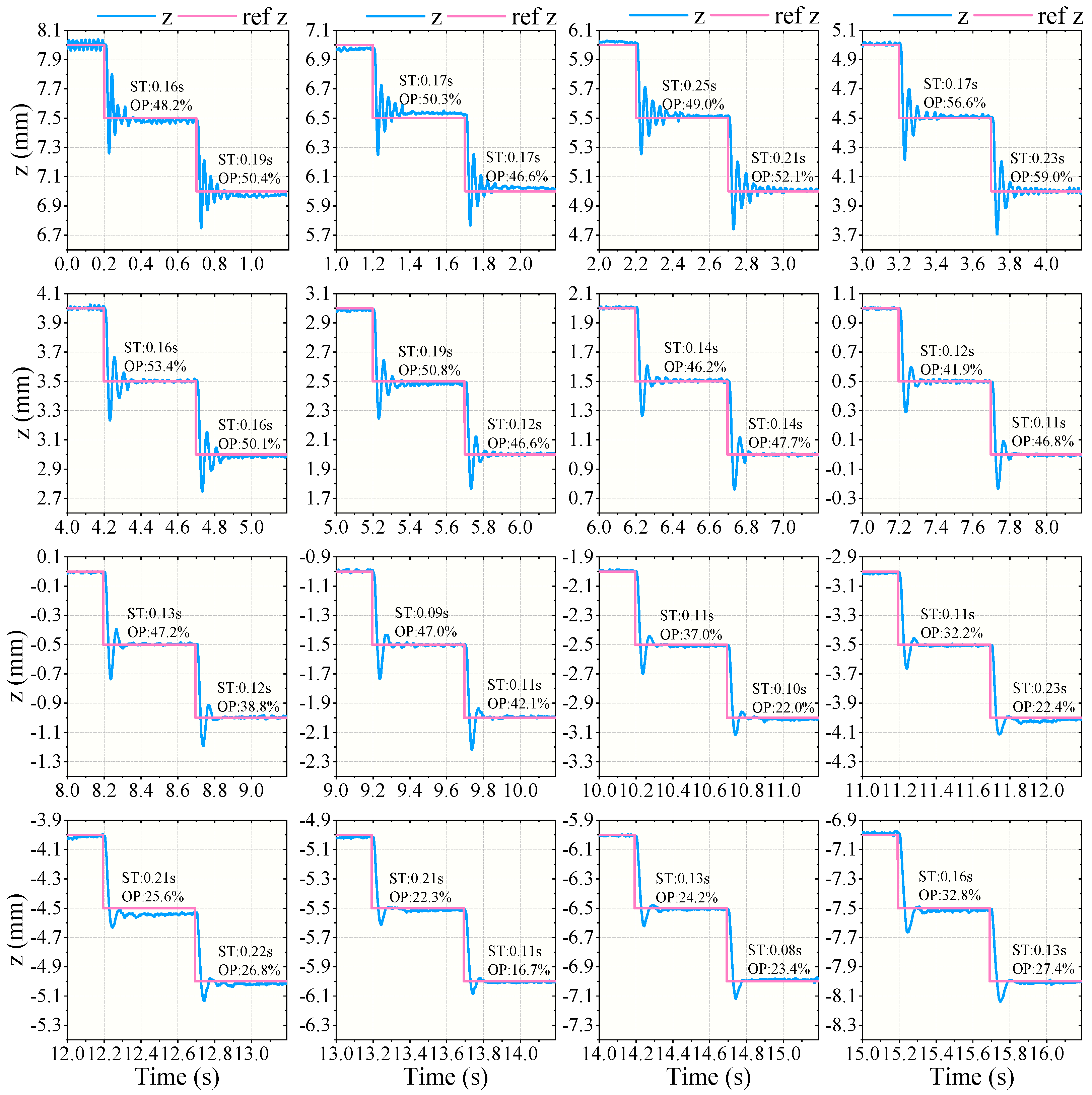
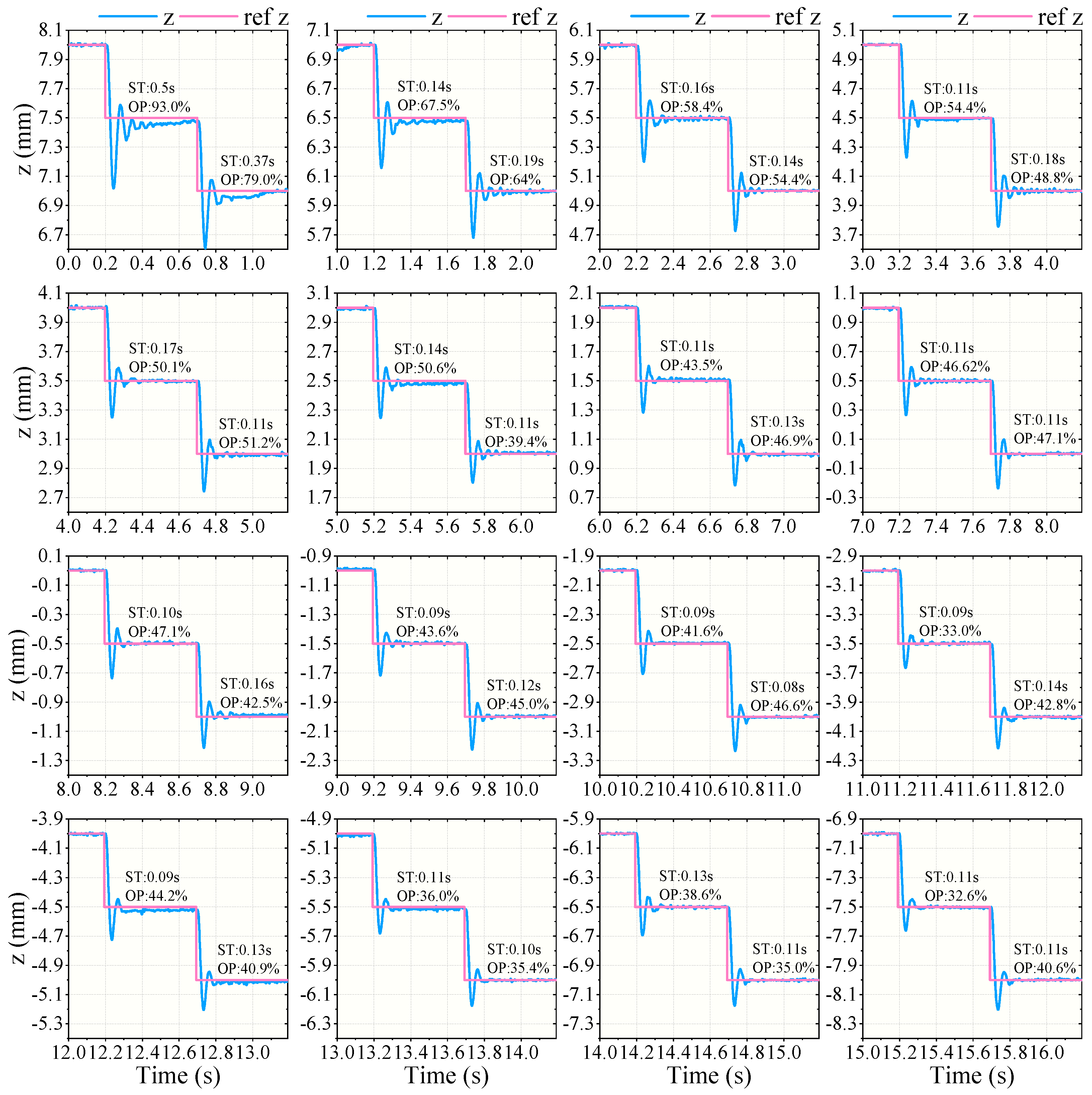
Finally, the feedforward scheme is integrated with the gain scheduling PID, and the resulting control strategy shown in Figure 7 is employed for the long-stroke levitation experiments. To compensate in real time for the feedforward error caused by modeling inaccuracies, the integral gain is also set to 1000. Afterwards, a 32-segment step input is applied to the reference displacement, and the step response results are shown in Figure 12. In each 0.5 mm step response, the settling time remains below 0.2 s, which is similar to that of the second control configuration. Meanwhile, the oscillations at small air gaps are effectively suppressed. Except for the relatively larger overshoot within the initial 1 mm air gap range, the control system exhibits uniform dynamic performance over the full stroke. This indicates that the scheduling proportional and the scheduling derivative gains effectively reduce the differences in equivalent stiffness and equivalent damping during long-stroke motion. Due to modeling inaccuracies caused by leakage flux at large air gaps, the control performance remains unsatisfactory. Nevertheless, this control strategy still offers notable advantages: the controller parameters can be derived directly from the actuator parameters, and the dynamic performance of the control system can be configured in an intuitive manner. Without recourse to empirical tuning, practitioners can effectively avoid the strong integral-gain dependence or excessively long settling times exhibited in the basic control configuration. In addition, the control strategy improves small-gap robustness and large-gap tracking without compromise.

5.3. Frequency Response Analysis

To further clarify the effect of the gain scheduling PD compensator on long-stroke positioning control, frequency response measurements are conducted. The frequency response analyzer (FRA-5022, NF Corporation, Tokyo, Japan) is used in the experiments, which generates sinusoidal signals at various frequencies and measures the feedback signal to obtain the Bode plot of the feedback control system. The sinusoidal signal is applied to the reference input of the control configuration via the analog input channel of the rapid prototyping system, while the levitation body’s real displacement is returned via an analog channel as feedback, yielding a frequency response equivalent to the complementary sensitivity T j ω . The RMS value of the sinusoidal reference input is 0.05 mm, which corresponds to a motion amplitude of ±0.0707 mm. After levitation positioning control is enabled and the steady-state error is eliminated, the frequency response measurements are performed. During the 16 mm displacement stroke, one measurement point is selected every 2 mm, yielding 9 measurement points in total.
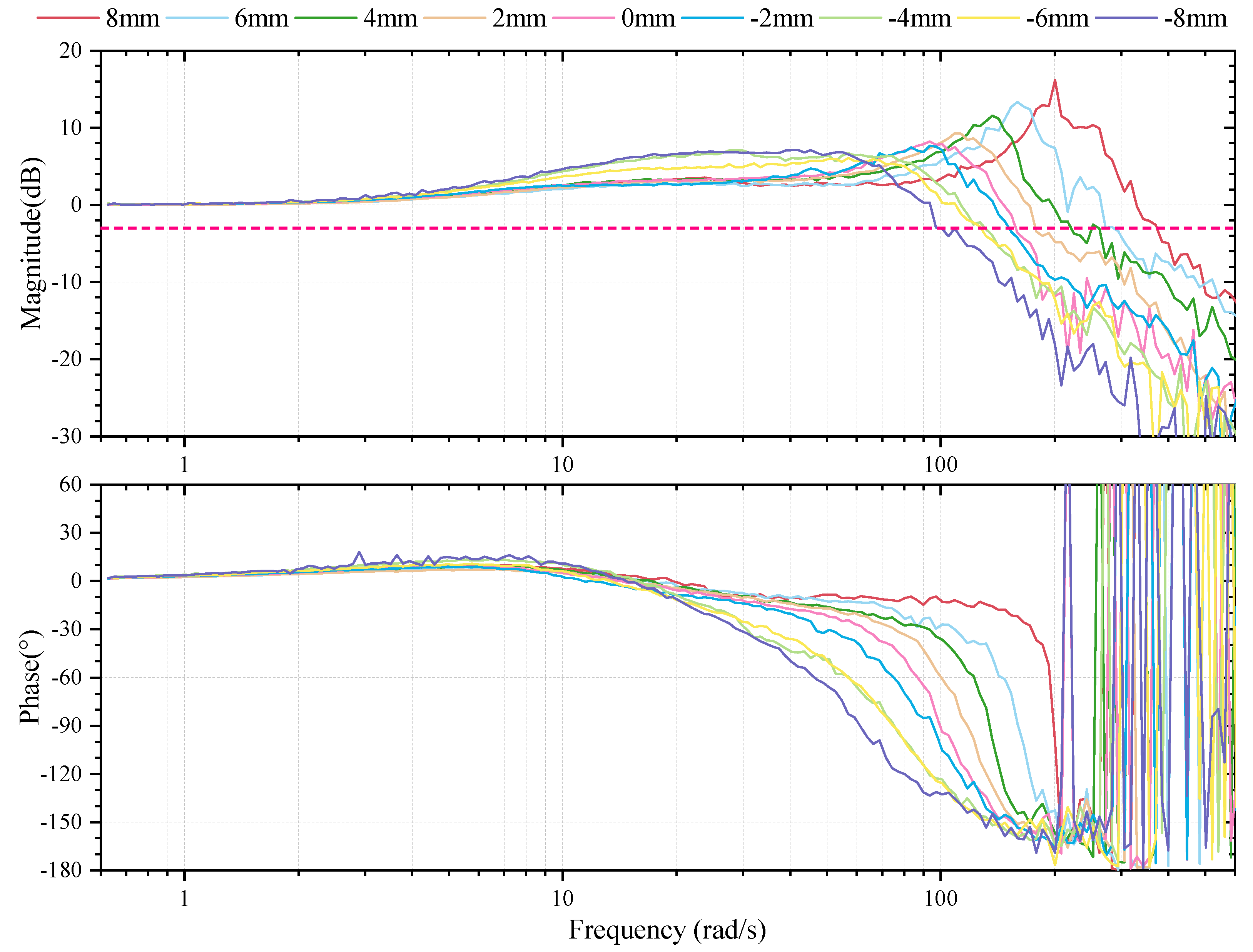
First, the basic feedback control configuration is measured, using the same parameters as in Section 5.2. The experimental results in Figure 13 show that all curves lie close to 0 dB at low frequencies, indicating uniform steady-state tracking gain across measurement points and suppressed steady-state error. In the mid-frequency region, resonance peaks are observed. Their magnitude is roughly + 5 to + 15 dB depending on measurement points, and the peak location also shifts slightly as the measurement point changes. In the high-frequency band, the magnitude of each curve decays rapidly and the phase drops sharply. To clearly illustrate how the frequency response varies across measurement points, the key performance indicators are summarized in Table 2. Due to factors such as measurement signal-to-noise ratio, the phase exhibits jitter. At small air gaps, the resonance peaks are higher and the crossover frequency shifts to the right, reflecting increased equivalent stiffness and a reduced damping ratio. As the air gap becomes larger, the peak is reduced and the bandwidth decreases slightly, consistent with a lower equivalent stiffness and a higher damping ratio.
Accordingly, the sensitivity S j ω , as the complement of the T j ω , shifts its corner frequency to higher values as the air gap decreases. As analyzed in Section 3.4 using the Bode sensitivity integral theorem, a rightward shift of the corner frequency necessarily elevates the sensitivity peak. Notably, at small air gaps the real part of the unstable pole is inherently larger. Under the ”waterbed effect”, the enlarged penalty area further elevates the sensitivity in the mid-to-high frequency band, which degrades robustness and reduces stability margins. In contrast, under the large air gap that more readily affords stability margins, the measurement results indicate that sensitivity is markedly suppressed, though at the expense of tracking performance.
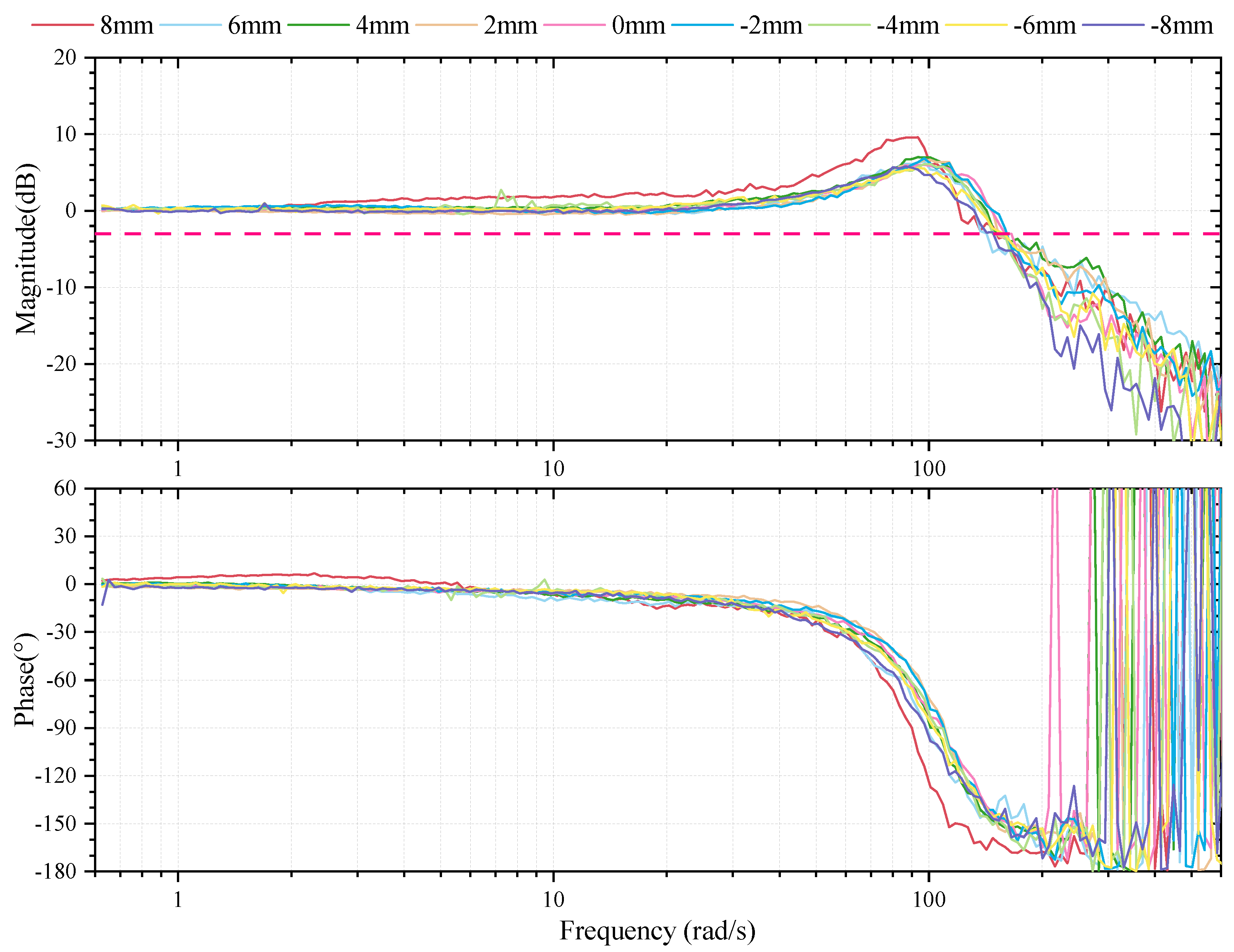
The frequency response measurements of gain scheduling strategy are presented in Figure 14. With scheduling proportional and derivative gains, the closed-loop Bode curves remain at 0 dB in the low-frequency band, indicating suppressed steady-state error across the full stroke and good low-frequency tracking performance. In the mid-frequency band, the resonance curves are clearly modified relative to the basic control configuration, and the key frequency-response indicators are reported in Table 3. Apart from the measurement point of minimum air gap, where nonlinearity and other factors lead to a slightly higher resonance of 9.6 dB, the resonance levels at the remaining points fall within 5.512 to 6.996 dB. The drift of the resonance peak with displacement is diminished, eliminating the previously observed right shift in Figure 13. Consequently, the closed-loop bandwidth remains uniform across different air gaps, thereby significantly enhancing the consistency of feedback performance over the entire stroke. The results show that, with gain scheduling, the conflict between robustness at small air gaps and tracking at large air gaps is effectively resolved, rather than remaining a trade-off. Furthermore, if a higher bandwidth and better tracking control performance are desired, it suffices to configure the stiffness ratio and damping ratio. Conversely, to lower the bandwidth and increase robustness, the same two parameters can be adjusted.

6. Conclusions and Further Research

This paper analyzes the control characteristics of the long-stroke reluctance maglev systems, and a gain scheduling strategy for positioning control is designed. Based on theoretical analysis and experimental validation, the following conclusions are obtained.
(1)
With basic PD/PID control, the equivalent stiffness and damping of reluctance maglev systems increase as the air gap decreases. As a result, the tracking performance becomes markedly nonuniform over the full stroke: small air gaps produce rapid responses with noticeable oscillations, while large air gaps result in low stiffness and deteriorated tracking.
(2)
From the robustness viewpoint, the Bode sensitivity integral theorem places inherent constraints on the relative stability of the reluctance maglev system. With decreasing air gap, the unstable pole acquires a larger real part, so high robustness is naturally harder to attain. Both analysis and experiments show that the basic PD/PID compensator produces a higher corner frequency and bandwidth at small air gaps, further degrading robustness. Conversely, at large air gaps, where high robustness is easier to secure, the corner frequency is reduced and tracking performance deteriorates. This suggests a clear trade-off between robustness and tracking performance over the full stroke.
(3)
The control strategy that combines feedforward with pole-placement adaptive PD is proposed and validated in time- and frequency-domain experiments. It does not rely on engineering experience, and the control gains are mapped directly from the actuator parameters. The experiments indicate that this control strategy effectively improves the consistency of control performance over the full stroke. These results further demonstrate that robustness at small air gaps and tracking performance at large air gaps are both enhanced, and the conflict between them over the long stroke is effectively mitigated rather than compromised.
Further research work includes extending the control strategy to multi-DOF maglev systems, and employing an extended state observer to estimate the levitated load so that load variations are explicitly accounted for in the control design. Moreover, a comprehensive robustness analysis of the gain scheduled system is necessary to quantify the influence of parameter perturbations, such as levitated-mass variations, on the closed-loop performance.

Author Contributions

W.P.: methodology, validation, software, writing—original draft preparation; C.Z.: Conceptualization, data curation, formal analysis, writing—review and editing; K.O.: supervision, resources, writing—review and editing; F.S.: resources, project administration, funding acquisition; J.J.: investigation, visualization; X.Z.: supervision, methodology. All authors have read and agreed to the published version of the manuscript.

Funding

This work was supported by the National Key R&D Program of China (Grant No. 2024YFB3410002), National Natural Science Foundation of China (Grant Nos. 52375258 and 52405284), China Postdoctoral Science Foundation (Grant No. 2024M762160), Scientific Research Fund Project of Liaoning Provincial Department of Education (Grant Nos. LJ222410142008, JYTMS20231191, and LJ212410142015), and China Scholarship Council Project (Grant No. 202408210076).

Institutional Review Board Statement

Not applicable.

Informed Consent Statement

Not applicable.

Data Availability Statement

The original contributions presented in this study are included in the article. Further inquiries can be directed to the corresponding author.

Conflicts of Interest

The authors declare no conflicts of interest.

References

  1. Lee, H.W.; Kim, K.C.; Lee, J. Review of maglev train technologies. IEEE Trans. Magn. 2006, 42, 1917–1925. [Google Scholar] [CrossRef] [Scilit]
  2. Wu, T.; Zhang, W. Review on Key Development of Magnetic Bearings. Machines 2025, 13, 113. [Google Scholar] [CrossRef] [Scilit]
  3. Du, Y.; Zhang, G.; Hua, W. Review on Research and Development of Magnetic Bearings. Energies 2025, 18, 3222. [Google Scholar] [CrossRef] [Scilit]
  4. Zhou, L.; Wu, J. Magnetic Levitation Technology for Precision Motion Systems: A Review and Future Perspectives. Int. J. Autom. Technol. 2022, 16, 386–402. [Google Scholar] [CrossRef] [Scilit]
  5. Pechhacker, A.; Wertjanz, D.; Csencsics, E.; Schitter, G. Integrated electromagnetic actuator with adaptable zero power gravity compensation. IEEE Trans. Ind. Electron. 2024, 71, 5055–5062. [Google Scholar] [CrossRef] [Scilit]
  6. Zhu, H.; Teo, T.J.; Pang, C.K. Magnetically Levitated Parallel Actuated Dual-Stage (Maglev-PAD) System for Six-Axis Precision Positioning. IEEE/ASME Trans. Mechatron. 2019, 24, 1829–1838. [Google Scholar] [CrossRef] [Scilit]
  7. Li, X.; Zhu, H.; Ma, J.; Teo, T.J.; Teo, C.S.; Tomizuka, M.; Lee, T.H. Data-Driven Multiobjective Controller Optimization for a Magnetically Levitated Nanopositioning System. IEEE/ASME Trans. Mechatron. 2020, 25, 1961–1970. [Google Scholar] [CrossRef] [Scilit]
  8. Dyck, M.; Lu, X.; Altintas, Y. Magnetically Levitated Rotary Table with Six Degrees of Freedom. IEEE/ASME Trans. Mechatron. 2017, 22, 530–540. [Google Scholar] [CrossRef] [Scilit]
  9. Kumar, D.; Sisodiya, M.S.; Bajpai, V. A novel servo-stabilized electromagnetic levitation formicro-EDM processing and its feasibility analysis. Proc. Inst. Mech. Eng. Part J Eng. Manuf. 2023, 237, 862–872. [Google Scholar] [CrossRef] [Scilit]
  10. Luan, B.; Zhang, X.; Xu, F.; Yang, G.; Jin, J.; Xu, C.; Sun, F.; Oka, K. High Precision Magnetic Levitation Actuator for Micro-EDM. Actuators 2022, 11, 361. [Google Scholar] [CrossRef] [Scilit]
  11. Xu, S.; Sun, J.; Ren, H. Design of an Integrated Five Degrees-of-Freedom Magnetic Suspension System with Long-Stroke Motion. IEEE Trans. Energy Convers. 2025, 40, 3035–3044. [Google Scholar] [CrossRef] [Scilit]
  12. Ma, W.; Liu, G.; Le, Y.; Zheng, S. Stiffness Compensation Control for Centrifugal Compressors Based on Online Parameter Identification of Magnetic Bearings. IEEE Trans. Ind. Electron. 2023, 70, 9421–9431. [Google Scholar] [CrossRef] [Scilit]
  13. Ren, M.; Oka, K. Design of a Noncontact Bending Testing Device Using Magnetic Levitation Mechanism. IEEE Trans. Ind. Electron. 2024, 71, 1697–1707. [Google Scholar] [CrossRef] [Scilit]
  14. Cigarini, F.; Ito, S.; Troppmair, S.; Schitter, G. Comparative Finite Element Analysis of a Voice Coil Actuator and a Hybrid Reluctance Actuator. IEEJ J. Ind. Appl. 2019, 8, 192–199. [Google Scholar] [CrossRef] [Scilit]
  15. Pumphrey, M.; Alatawneh, N.; Al Janaideh, M. Modeling and analysis of reluctance motion system with asymmetrical air gaps. Rev. Sci. Instrum. 2022, 93, 075001. [Google Scholar] [CrossRef] [Scilit]
  16. Pumphrey, M.; Al Saaideh, M.; Kuchinkaa, K.; Alatawneh, N.; Al Janaideh, M. Investigating the effect of the mean path length on reluctance actuator output force characterization. Rev. Sci. Instrum. 2022, 93, 115001. [Google Scholar] [CrossRef] [Scilit]
  17. Anthis, A.F., III. Six-Axis Levitated Stage with a Novel Flux-Steering Magnetic Hub Actuator. Master’s Thesis, Massachusetts Institute of Technology, Cambridge, MA, USA, 2021. [Google Scholar]
  18. Zhao, C.; Zhang, Q.; Pei, W.; Jin, J.; Sun, F.; Zhang, H.; Zhou, R.; Liu, D.; Xu, F.; Zhang, X.; et al. Design and Analysis of 5-DOF Compact Electromagnetic Levitation Actuator for Lens Control of Laser Cutting Machine. Micromachines 2024, 15, 641. [Google Scholar] [CrossRef] [Scilit]
  19. Pumphrey, M.; Saaideh, M.A.; Al-Rawashdeh, Y.M.; Alatawneh, N.; Xu, B.; Janaideh, M.A. A Novel 2-DoF Reluctance Electromagnetic Precision Motion System: Design, Modeling, and Control. IEEE Trans. Instrum. Meas. 2025, 74, 3004418. [Google Scholar] [CrossRef] [Scilit]
  20. MacKenzie, I. Design and Control Methods for High-Accuracy Variable Reluctance Actuators. Ph.D. Thesis, Massachusetts Institute of Technology, Cambridge, MA, USA, 2015. [Google Scholar]
  21. Al Saaideh, M.; Pumphrey, M.; Alatawneh, N.; Al Janaideh, M. On Electromagnetic Variable Air-Gap Reluctance Actuator Motion System: Characterization, Modeling, and Feedforward Control. IEEE/ASME Trans. Mechatron. 2024, 29, 3981–3992. [Google Scholar] [CrossRef] [Scilit]
  22. Wang, J.; Zhao, L.; Yu, L. Adaptive Terminal Sliding Mode Control for Magnetic Levitation Systems with Enhanced Disturbance Compensation. IEEE Trans. Ind. Electron. 2021, 68, 756–766. [Google Scholar] [CrossRef] [Scilit]
  23. Wang, J.; Rong, J.; Yang, J. Adaptive Fixed-Time Position Precision Control for Magnetic Levitation Systems. IEEE Trans. Autom. Sci. Eng. 2023, 20, 458–469. [Google Scholar] [CrossRef] [Scilit]
  24. Xu, Y.; Shu, F.; Su, X.; Guo, L.; Han, S.; Yang, X. A composite neural network-based adaptive sliding mode control method for reluctance actuator maglev system. Neural Comput. Appl. 2023, 35, 15877–15890. [Google Scholar] [CrossRef] [Scilit]
  25. Peng, T.; Peng, H.; Li, R. Deep learning based model predictive controller on a magnetic levitation ball system. ISA Trans. 2024, 149, 348–364. [Google Scholar] [CrossRef] [Scilit] [PubMed]
  26. Liu, G.; Lu, Y.; Liu, Y.; Dong, Z.; Ye, Z. Research on two-dimensional external magnetic drive method of maglev ball based on force imbalance. Rev. Sci. Instrum. 2020, 91, 105003. [Google Scholar] [CrossRef] [Scilit] [PubMed]
  27. Ghosh, A.; Rakesh Krishnan, T.; Tejaswy, P.; Mandal, A.; Pradhan, J.K.; Ranasingh, S. Design and implementation of a 2-DOF PID compensation for magnetic levitation systems. ISA Trans. 2014, 53, 1216–1222. [Google Scholar] [CrossRef] [Scilit]
  28. Zhang, C.; Lu, Y.; Liu, G.; Ye, Z. Research on one-dimensional motion control system and method of a magnetic levitation ball. Rev. Sci. Instrum. 2019, 90, 115005. [Google Scholar] [CrossRef] [Scilit]
  29. Bojan-Dragos, C.A.; Precup, R.E.; Preitl, S.; Hergane, S.; Hughiet, E.G.; Szedlak-Stinean, A.I. Proportional-integral gain-scheduling control of a magnetic levitation system. In Proceedings of the 2016 20th International Conference on System Theory, Control and Computing (ICSTCC), Sinaia, Romania, 13–15 October 2016; pp. 1–6. [Google Scholar] [CrossRef] [Scilit]
  30. Almobaied, M.; Al-Nahhal, H.S.; Arrieta, O.; Vilanova, R. Design a Robust Proportional-Derivative Gain-Scheduling Control for a Magnetic Levitation System. Mathematics 2023, 11, 4040. [Google Scholar] [CrossRef] [Scilit]
  31. Gunter, S. Respect the unstable. IEEE Control Syst. Mag. 2003, 23, 12–25. [Google Scholar] [CrossRef] [Scilit]
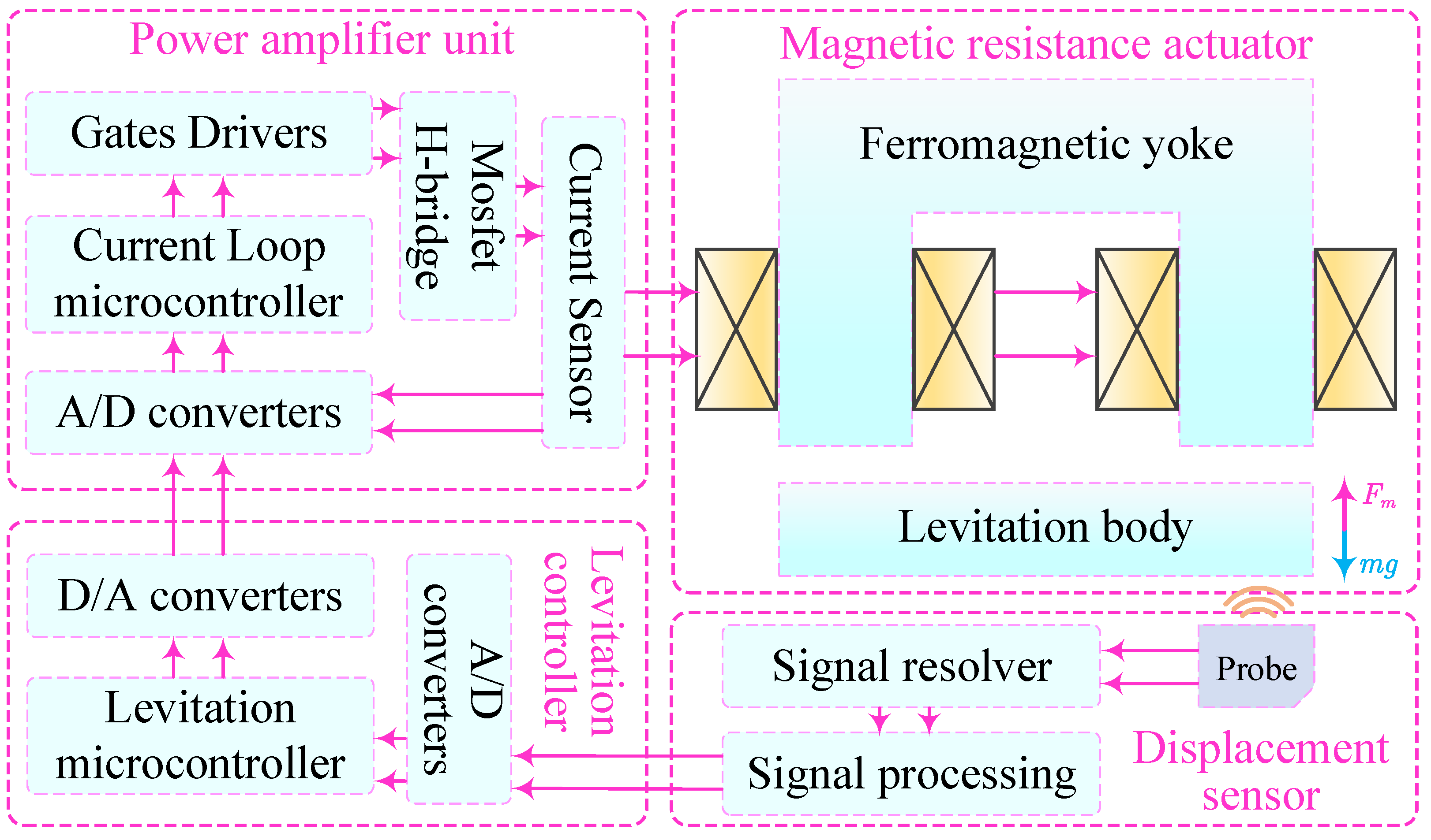
Figure 1. System components of reluctance maglev system.
Actuators 15 00151 g001
Figure 2. Diagram of magnetic flux path of C-type reluctance actuator.
Actuators 15 00151 g002
Figure 3. Basic feedback configuration of the reluctance maglev system. In this strategy, a standard PD/PID compensator and a fixed offset current i 0 i are used.
Actuators 15 00151 g003
Figure 4. Linear approximation of the feedback system.
Actuators 15 00151 g004
Figure 5. Diagram of the root locus clusters. (a) root locus with respect to k P when k D = 0 ; (b) root locus with respect to k D when k P is fixed at the marginally stable value.
Actuators 15 00151 g005
Figure 6. The diagram of ideal sensitivity profile. It is employed to derive Equations (41) and (42).
Actuators 15 00151 g006
Figure 8. Prototype of long-stroke reluctance maglev system.
Actuators 15 00151 g008
Figure 9. Mechatronics system for experiments.
Actuators 15 00151 g009
Figure 10. Step response results with basic feedback configuration. The motion proceeds from 2 mm to 18 mm of air-gap length with a step amplitude of 0.5 mm, yielding 32 steps to cover the entire stroke. ST: Setting time, OP: Overshoot percentage.
Actuators 15 00151 g010
Figure 11. Step response results with basic feedback configuration and feedforward. The motion is commanded from an air-gap length of 2 mm to 18 mm with a step size of 0.5 mm, giving a total of 32 steps to span the entire stroke. ST: Setting time, OP: Overshoot percentage.
Actuators 15 00151 g011
Figure 12. Step response results with feedforward and gain scheduling control strategy. In long-stroke positioning control, the response exhibits high consistency. ST: Setting time, OP: Overshoot percentage.
Actuators 15 00151 g012
Figure 13. Bode diagram of basic feedback configuration. At different measurement points, the resonance peaks, frequencies, and bandwidths exhibit significant disparities.
Actuators 15 00151 g013
Figure 14. Bode diagram of gain scheduling control strategy. With gain scheduling, the frequency responses across the measured points become highly consistent.
Actuators 15 00151 g014
Table 2. Key frequency-response performance indicators for the basic feedback configuration.
Measurement PointResonant FrequencyResonance PeakBandwidth
8 mm200.898 rad/s16.170 dB370.161 rad/s
6 mm159.756 rad/s13.344 dB283.315 rad/s
4 mm137.117 rad/s11.558 dB225.289 rad/s
2 mm113.279 rad/s9.246 dB179.152 rad/s
0 mm97.232 rad/s7.818 dB159.756 rad/s
−2 mm90.082 rad/s6.829 dB153.768 rad/s
−4 mm74.418 rad/s6.321 dB131.978 rad/s
−6 mm52.771 rad/s5.987 dB127.033 rad/s
−8 mm43.597 rad/s6.826 dB97.232 rad/s
Table 3. Key frequency-response performance indicators for the gain scheduling control strategy.
Measurement PointResonant FrequencyResonance PeakBandwidth
8 mm93.598 rad/s9.600 dB151.887 rad/s
6 mm97.232 rad/s6.847 dB142.458 rad/s
4 mm93.588 rad/s6.996 dB151.887 rad/s
2 mm101.014 rad/s6.159 dB153.768 rad/s
0 mm97.232 rad/s6.093 dB159.756 rad/s
−2 mm97.232 rad/s6.847 dB159.756 rad/s
−4 mm101.014 rad/s6.083 dB148.007 rad/s
−6 mm97.232 rad/s5.512 dB159.756 rad/s
−8 mm86.708 rad/s5.777 dB142.459 rad/s
Disclaimer/Publisher’s Note: The statements, opinions and data contained in all publications are solely those of the individual author(s) and contributor(s) and not of MDPI and/or the editor(s). MDPI and/or the editor(s) disclaim responsibility for any injury to people or property resulting from any ideas, methods, instructions or products referred to in the content.