Active Fault-Tolerant Method for Navigation Sensor Faults Based on Frobenius Norm–KPCA–SVM–BiLSTM

Abstract

Aiming to address the safety and stability issues caused by typical faults of Unmanned Aerial Vehicle (UAV) navigation sensors, a novel fault-tolerant method is proposed, which can capture the temporal dependencies of fault feature evolution, and complete the classification, prediction, and data reconstruction of fault data. In this fault-tolerant method, the feature extraction module adopts the FNKPCA method—integrating the Frobenius Norm (F-norm) with Kernel Principal Component Analysis (KPCA)—to optimize the kernel function’s ability to capture signal features, and enhance the system reliability. By combining FNKPCA with Support Vector Machine (SVM) and Bidirectional Long Short-Term Memory (BiLSTM), an active fault-tolerant processing method, namely FNKPCA–SVM–BiLSTM, is obtained. This study conducts comparative experiments on public datasets, and verifies the effectiveness of the proposed method under different fault states. The proposed approach has the following advantages: (1) It achieves a detection accuracy of 98.64% for sensor faults, with an average false alarm rate of only 0.15% and an average missed detection rate of 1.16%, demonstrating excellent detection performance. (2) Compared with the Long Short-Term Memory (LSTM)-based method, the proposed fault-tolerant method can reduce the RMSE metrics of Global Positioning System (GPS), Inertial Measurement Unit (IMU), and Ultra-Wide-Band (UWB) sensors by 77.80%, 14.30%, and 75.00%, respectively, exhibiting a significant fault-tolerant effect.

1. Introduction

In recent years, Unmanned Aerial Vehicles (UAVs) have been widely used in military, economic, and other fields because of their unique characteristics and superior performance, and have become a topic of interest in the field. However, with the rapid growth in the number of UAVs, potential risks such as interfering with civil aviation, unauthorized photography, and privacy infringement have emerged one after another. These issues have focused researchers’ attention on core matters including operational safety and security protection [1]. As one of the key core components of the UAV flight control system, navigation sensors play a crucial role in UAV flight safety, task execution, and other aspects [2]. However, navigation sensors are susceptible to interference during use because of various factors such as internal electromagnetic environment and severe weather, which can easily cause abnormal sensor feedback data and seriously affect the safety and stability of UAV flight [3]. Therefore, adopting appropriate fault-tolerant techniques to handle faults after detection is important to avoid the damage caused by sensor failures to system stability. This approach plays a crucial role in improving the stability of the UAV flight control system and ensuring flight safety [4,5,6].

In UAV flight control, fault-tolerant technology is a mechanism that ensures that the system can still operate normally or acceptably when some components fail. Currently, the fault-tolerant handling of UAV flight control system faults mainly includes passive fault tolerance and active fault tolerance [7,8]. Passive fault-tolerant technology mainly relies on robust control, adaptive control, and other measures to ensure that the system can operate in a stable state, and it is a commonly used fault-tolerance solution for eliminating UAV failures. For example, Saied et al. [9] studied the detection and isolation issues of actuator failure in multirotor UAV and proposed the use of robust control technology to address actuator failure problems without requiring fault detection scheme information. Nasiri et al. [10] proposed an adaptive passive fault-tolerant control method for actuator faults in affine Multi-Input Multi-Output (MIMO) nonlinear systems based on sliding mode control. Active fault-tolerant control has important practical value as a means of controlling and adjusting UAV fault states. For example, Bhatt et al. [11] proposed a hybrid fusion algorithm that uses Dempster-Shafer theory combined with Support Vector Machine (DS–SVM). DS–SVM utilizes DS theory to fuse Inertial Navigation System (INS) and Global Positioning System (GPS) data and models INS errors through SVM, thereby improving positioning accuracy. Ren et al. [12] proposed a fault-tolerant strategy based on local information, which can effectively compensate for the effect of actuator failure in each individual agent on the system. Lin et al. [13] used the backstepping sliding mode fault-tolerant control strategy to control the leader-follower multiagent system and successfully realized the control of the system.

With the development of intelligent technology, machine learning and deep learning have been applied in the fault prediction and fault-tolerant technologies of UAVs. Fu et al. [14] proposed a hybrid convolutional neural network (CNN)–long short-term memory (LSTM) model for actuator fault diagnosis of multirotor UAVs, which achieved an average fault diagnosis accuracy of 92.74%. Chen et al. [15] proposed an error compensation method for the Global Navigation Satellite System (GNSS)/INS integrated navigation system, which is based on an LSTM network integrated with an attention mechanism. In the scenario of 60-s GNSS signal interruption, the positioning accuracy of the system is improved by more than 90%. Guo et al. [16] constructed an intelligent active fault-tolerant system, which achieved a fault detection rate of 93% in an experiment with 150 groups of test samples. Wang et al. [17] proposed an LSTM-based one-class support vector machine (LSTM–OCSVM) hybrid model for detecting abnormal data from UAV sensors. The experimental results showed that the average detection rate and average accuracy of the model were 91.1% and 90.68%, respectively. Wu et al. [18] proposed a CNN–LSTM–Butterworth filter (CNN–LSTM–BF) hybrid model for UAV sensor anomaly detection, which achieves an average diagnostic accuracy of up to 96.50% in the scenario of sensor deviation anomalies.

In recent years, although UAV fault diagnosis and active fault-tolerant control technologies have been extensively studied, existing research has primarily focused on actuator faults, while studies on navigation sensor fault tolerance remain relatively scarce. Most current sensor fault tolerance solutions only address unidirectional temporal dependencies, failing to fully model the bidirectional temporal dependencies within sensor data. Moreover, some approaches suffer from high computational complexity and weak feature interpretability. In this study, these limitations have been addressed by exploring the design of a multisource sensor fault tolerance method. This approach can optimize actuator operation, reduce unnecessary starts and stops, improve the operational stability and prolong the service life of the actuators by monitoring sensor data in real time, filtering reliable perception information, and preventing faulty data from propagating to actuators.

To address the above challenges, this study proposes a novel active fault-tolerant method based on FNKPCA–SVM–BiLSTM. This method deeply integrates the Frobenius Norm (F-norm) with Kernel Principal Component Analysis (KPCA) to enhance the robustness of nonlinear feature extraction and reduce the rates of missed detection and false alarm; introduces an SVM classifier to achieve high-precision fault identification and enhance the reliability of system fault responses; and leverages the Bidirectional Long Short-Term Memory (BiLSTM) network to capture the bidirectional temporal dependencies of fault features, realizing the leap from “passive detection” to “active fault tolerance”. The core innovations and values of this method are as follows:

• The FNKPCA feature extraction method is proposed. The focus is on the inherent defects of traditional KPCA, such as high computational cost and poor feature interpretability. Integrating the F-norm with kernel principal component analysis improves the robustness of nonlinear feature extraction and reduces the interference of redundant information.
• The FNKPCA–SVM fusion detection strategy is constructed to reduce computational complexity and improve the efficiency of abnormal data detection.
• The “detection trigger–prediction response” collaborative mechanism is designed. Combined with the bidirectional time-series dependence characteristics of sensor data, BiLSTM is introduced to capture the bidirectional time-series correlation of fault features, the comprehensive modeling of dynamic processes is realized, and fault prediction accuracy and fault-tolerant effectiveness are improved.
• In terms of the practical application level, the focus is on the fault-tolerant processing of UAV navigation sensor faults.

2. FNKPCA–SVM–BiLSTM Active Fault-Tolerant Model

For systematically analyzing the technical implementation logic of the fault-tolerant model, this section will elaborate on the complete execution steps from fault detection to data reconstruction, focusing on three aspects: the model framework, the fault-tolerant method process, and the bidirectional temporal prediction network for sensor data.

2.1. Model Composition

During UAV flight control, complex electromagnetic environments or adverse weather conditions (such as heavy rain, thunderstorms, high ionospheric activity, and strong winds) can cause differential interference to various navigation sensors. Specifically, under heavy rainfall conditions, satellite signals are significantly affected by ionospheric refraction and multipath effects, which easily lead to a substantial degradation in the accuracy of the GPS. In strong wind environments, drastic attitude changes of the UAV trigger high-frequency dynamic movements, resulting in a significant increase in the measurement noise of the Inertial Measurement Unit (IMU). Such weather-induced sensor anomalies directly interfere with UAVs’ attitude control algorithms, resulting in trajectory deviations from the intended path and compromising mission stability and safety.

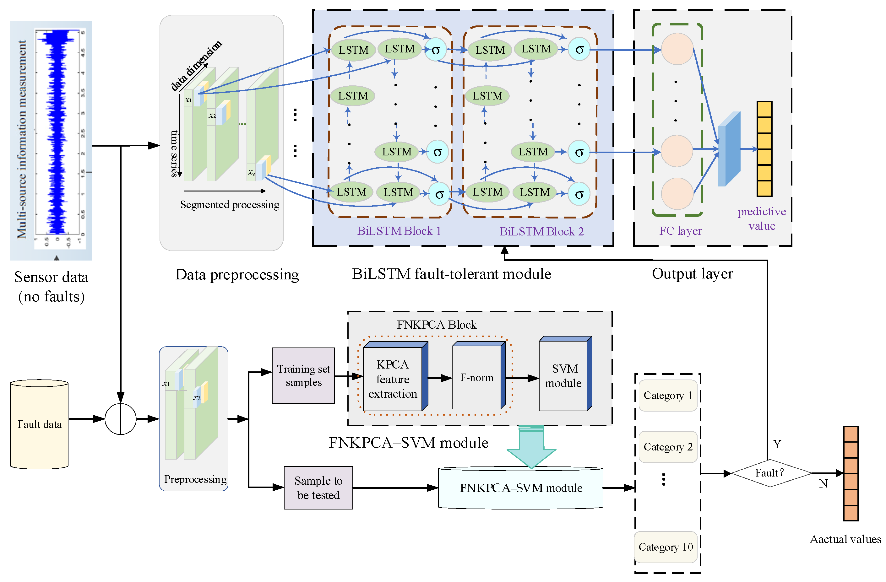
Damage to the system stability caused by sensor failure can be avoided and the UAV can be ensured to still meet the normal flight state after fault detection by applying fault-tolerant compensation processing to allow the UAV to realize safe flight in a short time, enabling it to perform return or landing operations and ensuring its safety [5]. Therefore, on the basis of the concept of fault-tolerant strategies, an active fault-tolerant model with FNKPCA–SVM fault detection and BiLSTM prediction network as the core is constructed, including an input module, a FNKPCA–SVM-based fault detection module, a BiLSTM-based multiscale fault-tolerant module, and an output module (Figure 1).

The overall process of the active fault-tolerant method is as follows: First, multi-dimensional time-series data are collected from the navigation sensor outputs, including the east, north, and sky position information of the GPS, the three-axis acceleration and angular velocity information of the IMU, and the ranging information of an Ultra-Wide-Band (UWB) sensor, which are preprocessed and used as the input of the subsequent feature extraction module. Second, the FNKPCA–SVM fault detection module is constructed to extract the characteristics of abnormal changes in a deep level. Third, the long-term dependence in the evolution process of fault characteristics is obtained by constructing a multiscale active fault-tolerant module with a BiLSTM network as the core unit, and fault-tolerant processing of fault signals is realized. Finally, the corresponding fault-tolerant results are obtained through the output module.

2.2. Active Fault-Tolerant Method Process

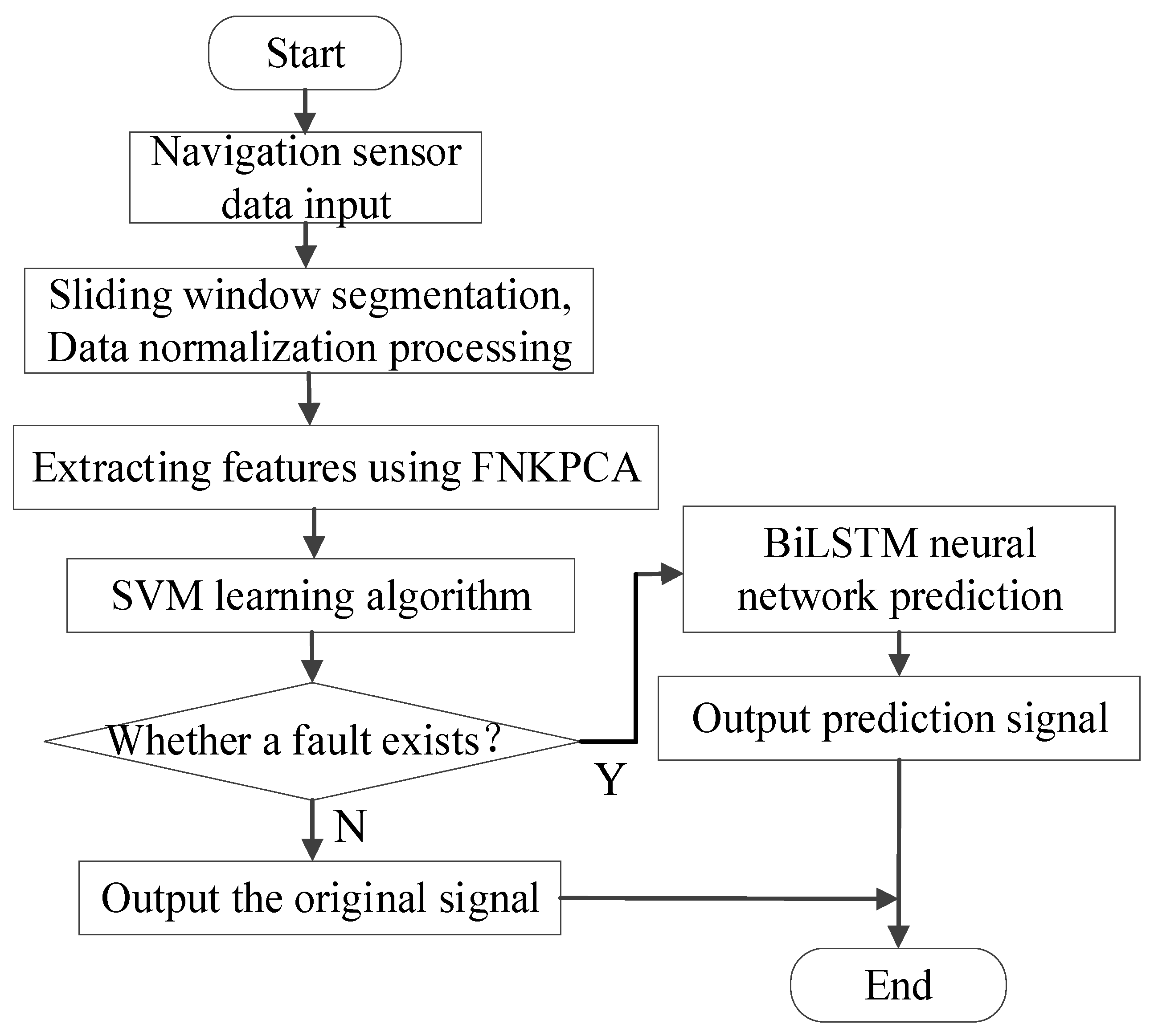
The active fault-tolerant method implemented based on FNKPCA–SVM and combined with the BiLSTM network is mainly divided into five stages: data input, data preprocessing, feature extraction, fault detection, and dynamic fault prediction. Figure 2 shows the flowchart of the active fault-tolerant method.

The specific steps are as follows:

• Data input: First, the navigation sensor data are received.
• Data Preprocessing: The data are segmented using a window approach, and then preprocessing is completed using min-max normalization.
• Feature Extraction: The preprocessed data are subjected to feature extraction using the FNKPCA method.
• Fault Detection: The extracted features are input into the trained SVM model for fault detection. If the SVM detects no fault in the sensor data, then it will directly output the original signal of the sensor. If the SVM detects a fault in sensor data, then the process will proceed to step (5).
• Dynamic Prediction: The effective data of the first three moments before the fault point are located and input into the BiLSTM neural network for prediction. For example, when an abnormal observation value x_t is detected at time t, the BiLSTM fault-tolerant prediction model of the corresponding sensor is automatically activated. The sliding window data (x_t−3, x_t−2, x_t−1) from the first 3 s at the fault moment are extracted as input, and the predicted value y_t of the fault time is calculated through forward propagation. If a short-term continuous fault occurs, such as when a fault is detected at time t + 1, then a recursive method is used for dynamic prediction. The predicted value y_t at time t is used as the end data point of the sliding window at time t + 1. At this time, the input data of the BiLSTM fault-tolerant prediction model are changed to (x_t−2, x_t−1, x_t), and the predicted output of the BiLSTM fault-tolerant model is y_t+1.

Through the above active fault-tolerant strategy, sensor faults can be effectively identified, and BiLSTM can be used for dynamic reconstruction to generate predicted values instead of abnormal data, thereby ensuring the robustness of UAV flight control systems in complex environments.

2.3. Bidirectional Temporal Prediction Network Algorithm for Sensor Data

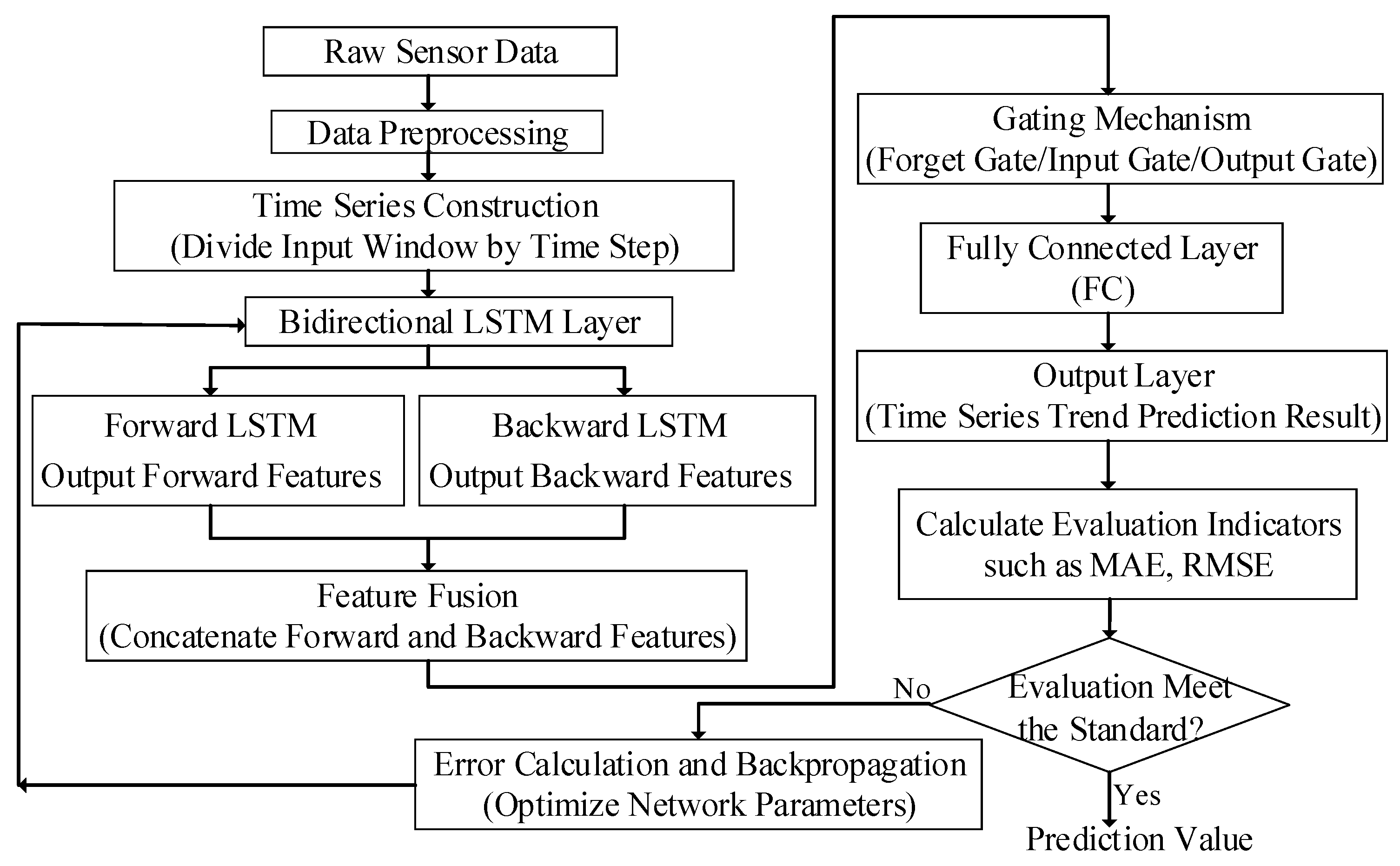
This algorithm takes the bidirectional LSTM as its core architecture. It accurately captures the bidirectional long-term dependencies of time-series data through a gating mechanism and then combines the closed-loop iterative strategy of “prediction–evaluation–optimization” to achieve efficient prediction of sensor time-series data (see the flowchart in Figure 3). It can be mainly divided into the following stages:

• Sensor Data Preprocessing: It includes the collection of raw sensor data and data preprocessing operations. This process aims to address issues such as data missing and anomalies, providing high-quality inputs for subsequent modeling.
• Sliding Window-Based Temporal Sample Construction: The input window is divided in accordance with the set time step. Through the sliding window, one-dimensional time-series data can be converted into multidimensional samples.
• Feature Extraction: This step is a core innovation. It mainly captures forward and reverse temporal dependencies simultaneously through bidirectional LSTM layers (forward and backward LSTM), resulting in comprehensive feature representations. Subsequent feature fusion involves concatenating forward and reverse features.
• Model Inference and Predicted Value Output: Temporal trend prediction results are obtained through gating mechanisms, fully connected layers, and output layers. Evaluation metrics such as Mean Absolute Error (MAE) and Root-Mean-Square Error (RMSE) are calculated to determine if the evaluation meets the standards. If so, the predicted values are output.
• Model Optimization: If the evaluation fails to meet the standards, error calculation and backpropagation are performed. After the network parameters are optimized, the results are fed back to the previous process for continued iteration.

Figure 3. Flowchart of the Bidirectional temporal prediction network for sensor data.

Figure 3. Flowchart of the Bidirectional temporal prediction network for sensor data.

3. Methods

In this subsection, the core components of the model will be elaborated in detail.

3.1. FNKPCA Feature Extraction Module

Numerous factors affect the reliability of navigation sensors in UAV flight control systems. These factors are interrelated to a certain extent, and most of them are nonlinear variables, which further reduces the prediction accuracy of the model and limits its generalization ability. The core of KPCA lies in extracting the principal component features of data with the help of kernel matrices [19,20]. However, this method does not constrain the overall energy distribution after the projection of principal components, and it easily loses global information due to fluctuations in local features. The F-norm can convert high-dimensional matrices into quantifiable scalars [21], and its introduction can overcome the shortcomings of the standard KPCA, which “emphasizes local features while neglecting global distribution.” In the scenario of sensor fault detection, this improvement can more accurately capture abnormal changes in data.

If a dataset of N samples exists in m-dimensional space: $x_i\in {\mathbb{R}}^m \left(\mathrm{1,2},\cdots ,N\right)$, then a mapping φ(•) that projects x into a higher-dimensional space needs to be found for linear analysis. Its covariance matrix C can be expressed as

$$C={\displaystyle \frac{1}{N}}\sum _{i=1}^N\phi \left(x_i\right)\phi {\left(x_i\right)}^T,$$

(1)

where φ(•) is the nonlinear mapping function from the input variable to the high-dimensional feature space.

Eigenvalues of the covariance matrix are solved as follows:

$$\lambda V=CV,$$

(2)

where λ is the eigenvalue of matrix C, and λ > 0; V is the eigenvector.

The kernel matrix ($K\in {\mathbb{R}}^{\mathit{N}\times \mathit{N}}$) and its element are defined to realize nonlinear data processing:

$$K_{ij}=K\left(x_i,x_j\right)=\langle \phi \left(x_i\right),\phi \left(x_j\right)\rangle (i,j=\mathrm{1,2},\cdots ,N),$$

(3)

where K_ij is the corresponding element, and K(x_i, x_j) is the kernel function. Given the obvious nonlinear structure of navigation sensor data in UAV flight control systems, the radial basis function (RBF) is chosen as the kernel function [22,23]:

$$K\left(x_i,x_j\right)=exp\left(-{\displaystyle \frac{1}{2{\sigma }^2}}{\Vert x_i-x_j\Vert }^2\right),$$

(4)

where σ² is the width parameter of the kernel function, σ > 0, and this positive parameter determines the measurement range of the RBF of the similarity between sample points x_i and x_j. Particularly, in the application scenarios of KPCA, when using the RBF kernel function, the data in the high-dimensional space must be centralized [20]. After this processing, a simplified expression of K can be obtained:

$$\tilde{K}=K-{\displaystyle \frac{1}{N}}{1}_{N}K-K{\displaystyle \frac{1}{N}}{1}_N+{\displaystyle \frac{1}{N^2}}{1}_{N}K{1}_N,$$

(5)

where $\tilde{K}$ is the centralized matrix, and 1_N is an N × N all-ones matrix.

Given Equations (2), (3) and (5), the following can be obtained:

$$N{\lambda }_i{\mathsf{\alpha }}_i=\tilde{K}{\mathsf{\alpha }}_i,$$

(6)

where α = (α₁, α₂, …, α_N)^T. The eigenvector α_i and the eigenvalue λ_i (i = 1, 2, …, N) can be solved by Equation (6).

In KPCA, the magnitude of eigenvalues reflects the importance of data information. The larger the eigenvalue, the more critical the corresponding data information. To identify the principal information factors, this study sets an 80% cumulative contribution rate as the threshold, determining the corresponding number of eigenvectors as the principal component count [24,25]. Finally, project the selected feature vectors into the principal component space to obtain the score matrix T, as shown below:

$$T=\tilde{K}{V}_{N\times p},$$

(7)

where V_N×p = [v₁, v₂, …, v_p] is a matrix composed of the first p eigenvectors. p is the number of extracted principal components, that is, the number of retained eigenvectors after the cumulative contribution rate reaches 80%, satisfying $1\le \mathrm{p}\le \min \left(\mathrm{r}\mathrm{a}\mathrm{n}\mathrm{k}\left(\tilde{K}\right),N\right)$.

The F-norm quantifies the total projection energy of data on all principal components by calculating the square root of the sum of the squares of all elements in the matrix. When the data are in a normal state, the distribution of projection energy on its principal components remains stable. However, when the sensor data contain faults, the data distribution will deviate from the normal pattern, and the corresponding F-norm of the score matrix will also fluctuate significantly. On the basis of this characteristic, the F-norm of the score matrix T can be calculated to determine whether the data are abnormal. Its calculation method is as follows:

$${\Vert \mathrm{T}\Vert }_F=\sqrt{\sum _{i=1}^N\sum _{j=1}^N{t}_{ij}^2},$$

(8)

where ‖T‖_F represents the F-norm, and t_ij represents any element in the score matrix T.

The distinction between normal and fault data relies on the judgment threshold determined on the basis of the statistical analysis of normal samples (the critical value corresponding to the 95% confidence interval). When data anomalies occur, their feature distribution deviates from the normal state, causing a shift in the principal component direction of KPCA. This shift is reflected by changes in the eigenvalues of the kernel matrix, which in turn makes the norm of the score matrix exceed the normal fluctuation range and becomes a key quantifiable indicator for fault detection.

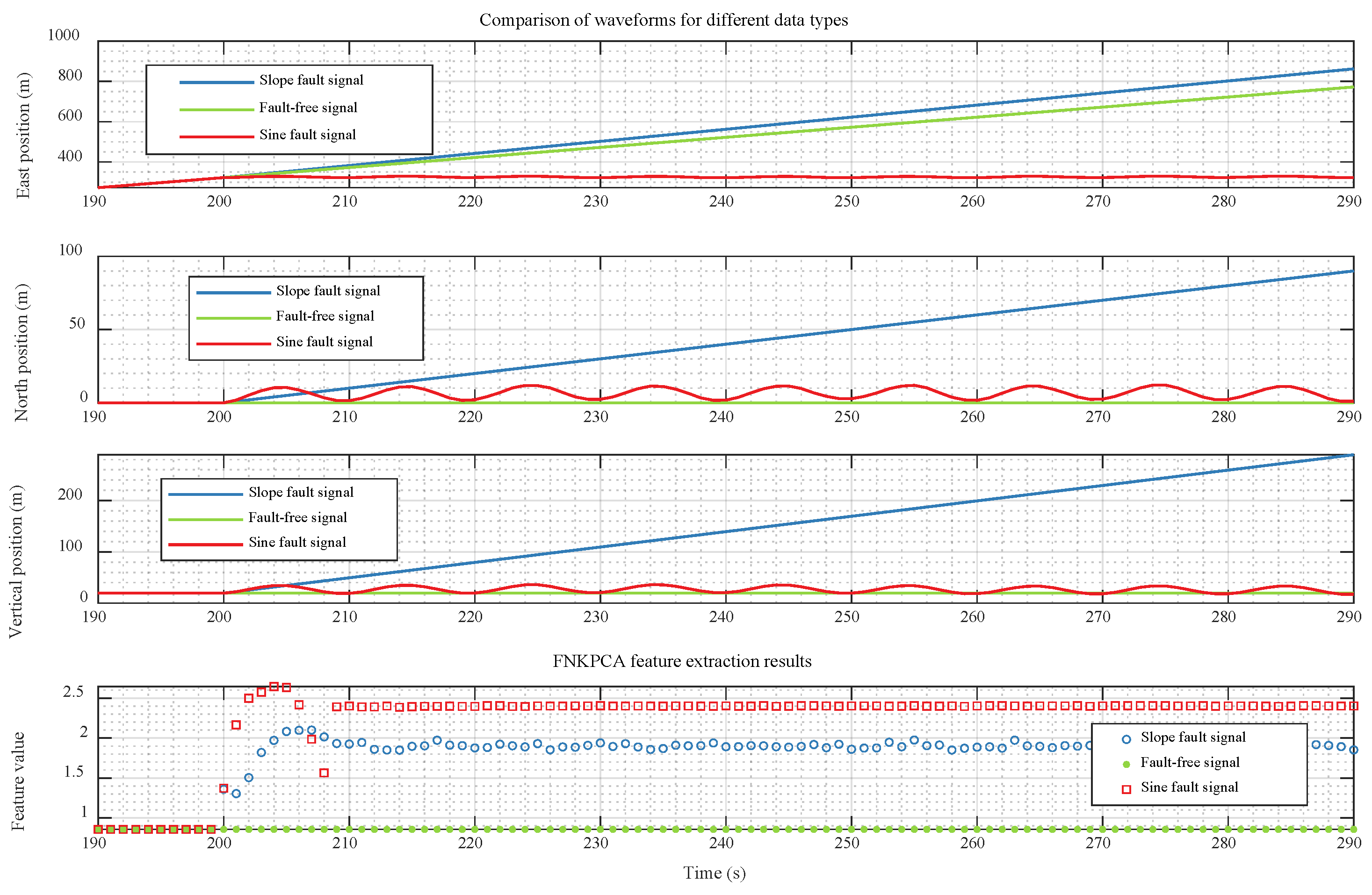
The FNKPCA feature extraction method ensures that fault or anomaly signals can be sensitively captured in complex sensor data, further improving the reliability and detection accuracy of the system. Taking the “GPS sensor” as an example, starting from the 200th second of the position information it outputs, the FNKPCA method is introduced to perform feature extraction on the fault-free signal, the slope fault signal, and the sine fault signal, respectively. Figure 4 shows the partial results of the feature extraction method based on FNKPCA.

3.2. Fault Detection Module

In the active fault-tolerant system of UAVs, quickly and accurately identifying abnormal flight states is the core objective, which highly depends on the fault detection and identification process after feature extraction from sensor data. As the core component of this link, the performance of the classifier directly determines the accuracy of fault identification. This study adopts SVM as the predetection module for fault-tolerant decision-making, which has obvious advantages. In particular, compared with the softmax classification algorithm of convolutional neural networks, SVM has stronger generalization ability for nonlinear and nonstationary data and better training efficiency [26]. Furthermore, through the design of regularization terms and kernel functions, SVM can effectively deal with small-sample nonlinear classification problems, which is highly consistent with the sensor fault identification requirements of UAV flight control.

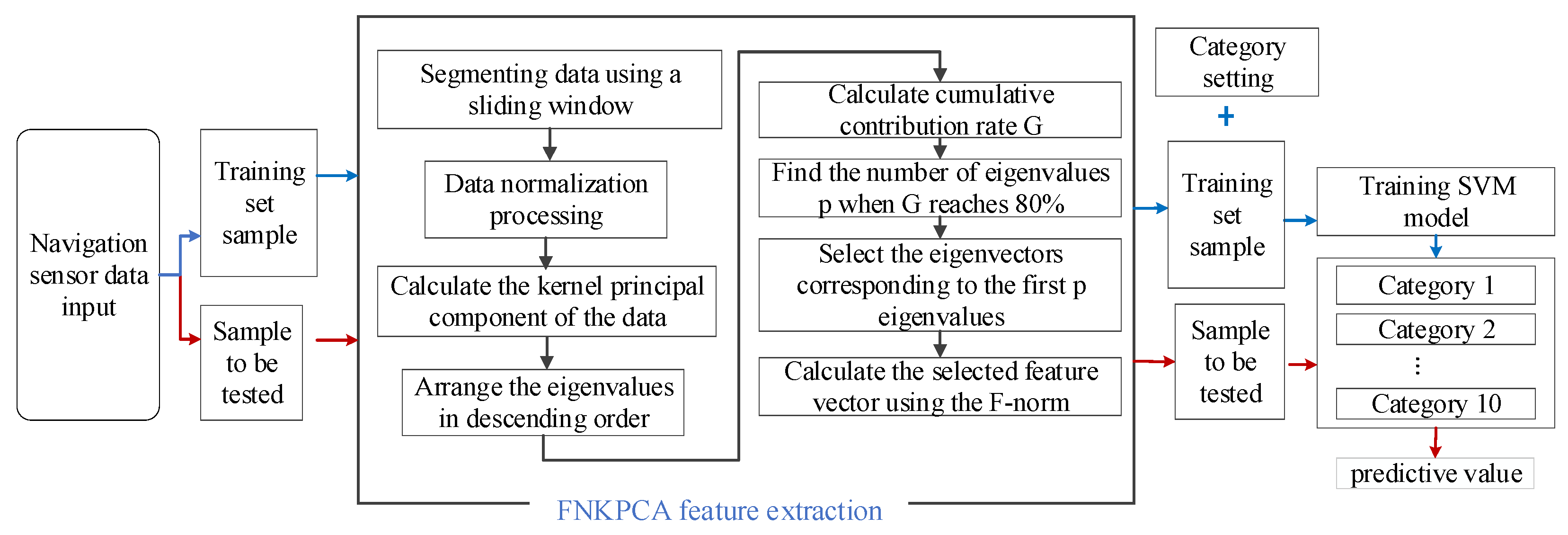
On this basis, this study constructs a fault detection module integrating FNKPCA and SVM. By leveraging the synergy between deep feature extraction and high-dimensional space classification, this module not only exerts the advantages of FNKPCA in nonlinear feature capture, redundant information filtering, and fault feature enhancement but also maximizes the classification capability of SVM, ultimately achieving a significant improvement in the accuracy of fault detection and prediction. The classification flowchart of the FNKPCA–SVM fault detection module is shown in Figure 5.

First, in accordance with the typical fault conditions of the UAV flight system, data collection nodes are set up in modules such as GPS, IMU, and UWB. After preprocessing operations such as noise reduction and normalization on the originally collected data, the training sample set and the to-be-detected sample set are divided at a ratio of 7:3 to provide a data foundation for subsequent module training. Next, FNKPCA maps the preprocessed navigation sensor data to a high-dimensional feature space through a kernel function. With the matrix measurement characteristics of the F-norm, it effectively captures the nonlinear coupling relationship between fault data and normal states, laying a foundation for SVM to construct accurate classification boundaries. Subsequently, on the basis of the feature vectors extracted by FNKPCA and the corresponding fault category labels, the SVM algorithm quickly learns clear “fault-normal” classification boundaries through iterative training with limited samples, ensuring the accuracy of multitype fault (Categories 1–10) prediction. Finally, the trained multiclassification model is applied to the fault prediction of the to-be-detected samples. The effects of different models are compared through multidimensional performance indicators, and the fault detection model with the highest prediction accuracy and strongest generalization ability is selected.

3.3. Bidirectional Sequence Feature Processing Network

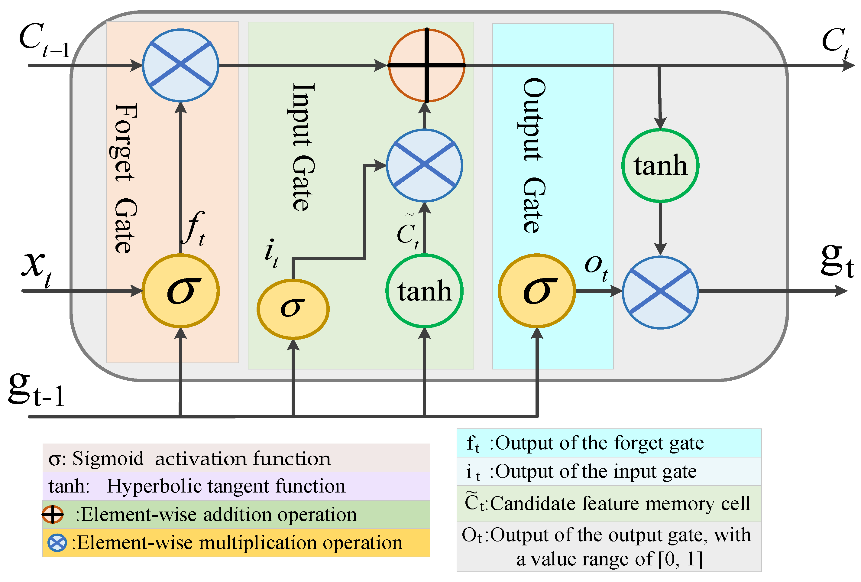
As a typical network for feature extraction, the LSTM network (Figure 6) mainly establishes the correlation analysis of feature information at different time points through the forget gate, input gate, and output gate [27].

Where x_t represents the feature information at time t processed by the multilevel feature extraction module, g_t indicates the feature information extracted by the LSTM network at time t, and C_t denotes the feature memory cell at time t.

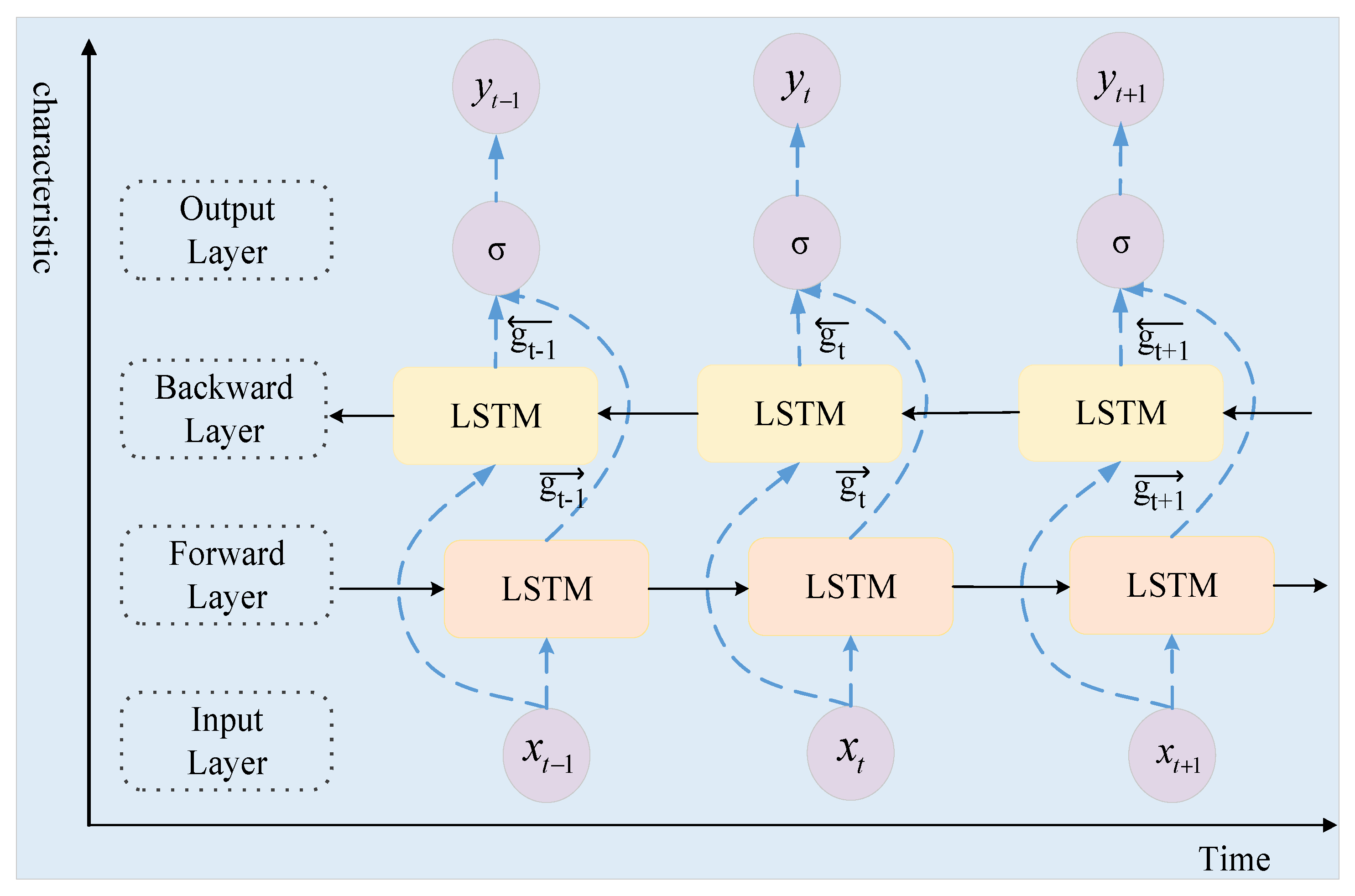
Important information in the feature data was obtained from different time and feature dimensions, and a sequence feature processing network based on BiLSTM [28] was constructed to achieve multi-level feature extraction of input information (Figure 7).

For BiLSTM, we have the following:

$$\{\begin{array}{c}\overrightarrow{g_t}=LSTM\left(x_t, \overrightarrow{g_{t-1}}\right),\\ \overleftarrow{g_t}=LSTM\left(x_t,\overleftarrow{g_{t-1}}\right),\\ y_t=\mathsf{\sigma }\left(W_y·\left[\overrightarrow{g_t},\overleftarrow{g_t}\right]+b_y\right),\end{array}$$

(9)

where $\overrightarrow{g_t}$ is the process feature information in the forward layer, and $\overleftarrow{g_t}$ is the process feature information in the backward layer. W_y and b_y are the weight matrix and bias term, respectively.

Specifically, with x_t taken as an example, it is sent into two LSTM units for processing. The forward LSTM layer extracts a feature over a shorter time period, while the backward LSTM layer captures a feature over a longer time period. Then, the output layer features y_t are further processed by the activation function σ. The multi-scale fault feature information obtained by concatenating the two temporal sequence directions mentioned above takes into account the influence of past and future information on the current moment, thereby helping the model achieve higher fault diagnosis accuracy.

4. Experiment

Three aspects of the model—establishment of fault dataset, fault prediction comparison analysis, and active fault-tolerant comparison analysis—are presented to demonstrate the effectiveness of the FNKPCA–SVM–BiLSTM model structure and objectively evaluate its performance.

4.1. Dataset Establishment and Parameter Configuration

The open source dataset used in this study was collected by a university team through a sports car moving on the university campus, including sensor data from a STIM300 inertial measurement unit, a single-point GNSS receiver, and an inertial-grade fiber-optic gyroscope (FOG) system. The GNSS sampling frequency is 1 Hz, the STIM300 sampling frequency is 125 Hz, the data collection duration is approximately 50 min, and the corresponding total number of samples is approximately 375,000, which comprises inertial measurement data and GNSS positioning data. In addition, UWB data simulate the dynamic range values of UAVs by real-time outputting the virtual range information between the set UWB module and the mobile car.

Typically, navigation sensor faults can be divided into two categories on the basis of the rate of fault signal change: abrupt and gradual faults. Combined with the typical fault conditions of actual systems, three types of faults are set as follows: (1) sine faults, (2) slope faults, and (3) sudden faults. In this study, fault data are generated by taking normal navigation sensor data as the benchmark and sequentially injecting preset faults at fixed intervals of 100 s within the time range of 2000–3000 s to form a multitype fault dataset. Fault parameter settings are shown in

Table 1. Fault parameter settings.

Sensor	Signal Type	Parameter Range	Key Function
GPS	fault-free signal	No	No
	sine fault signal	A1 ∈ [2, 6]; f1 ∈ [0, 10]; φ1 ∈ [0, 3π/4]	simulate complex periodic interference caused by multipath effects
	slope fault signal	k1 ∈ [−7, 7]	simulate positive and negative drift of signals due to ionospheric interference
	sudden fault signal	ζ1 ∈ [3, 7] m	simulate positioning deviation caused by signal occlusion/interruption
IMU	fault-free signal	No	No
	sine fault signal	A2 ∈ [0.2, 7]; f2 ∈ [0, 10]; φ2 ∈ [0, π/2]	simulate common periodic interference such as device vibration and circuit noise
	slope fault signal	K2 ∈ [−2.5, 2.5]	simulate gradual anomalies caused by device aging and temperature drift
	sudden fault signal	ζ2acc ∈ [0.05, 2] g; ζ2anv ∈ [1, 20] °/s	cover the full dynamic range
UWB	fault-free signal	No	No
	sudden fault signal	ζ3 ∈ [3, 7]	Simulate ranging value fluctuations caused by signal occlusion/multipath interference

.

In Table 1, parameter A represents the amplitude of the sine fault signal, f denotes the frequency, and φ stands for the phase; k is the parameter of the slope fault signal; ζ is the amplitude of the sudden fault signal.

On the basis of the normal data of the navigation sensor and the fault datasets with various fault types added (as listed in Table 1), first, the data are divided using a sliding window with a window size of 10 sampling points and a step size of 1 sampling point. The max–min normalization method is used to preprocess the data within the window, and then FNKPCA is combined to extract features to construct the model training set. To verify the model adaptability, the test set adopted different fault amplitudes from the training set and was formed after the same feature extraction process. The number of samples in the training and test sets for each signal type is shown in

Table 2. Distribution of signal samples and label classification.

Sensor	Signal Type	Training Sample	Test Sample	Class
GPS	fault-free signal	990	140	1
	sine fault signal	990	140	2
	slope fault signal	990	140	3
	sudden fault signal	990	140	4
IMU	fault-free signal	990	140	5
	sine fault signal	990	140	6
	slope fault signal	990	140	7
	sudden fault signal	990	140	8
UWB	fault-free signal	990	140	9
	sudden fault signal	990	140	10

.

The BiLSTM network model architecture designed in this study consists of one input layer, two BiLSTM layers, one fully connected layer, and one regression layer, in which each BiLSTM layer contains 64 hidden units. The initial learning rate is 0.005, the batch size is 32, the Adam optimizer is selected, and the training iterates 100 times in total. The specific parameter configuration is shown in

Table 3. Parameter configuration of the BiLSTM network model.

Hyperparameter	Parameter Range	Description
initial learning rate	0.005	controls the parameter update step size
optimizer	adam	adaptive learning rate optimization algorithm
number of BiLSTM layers	2	enhances the model’s feature capture ability
hidden layer	64	captures bidirectional information in time-series data
epoch	100	maximum number of iterations: 100
batch-size	32	number of samples used per iteration
gradient threshold	1	prevents gradient explosion

.

In the stacking of 2 BiLSTM layers, the first BiLSTM layer completes the extraction of dynamic features of the entire sequence, ensuring the complete capture of contextual information in the sensor time-series data. The second BiLSTM layer only extracts the hidden state of the last time step, which not only condenses the global time-series information into a single key feature vector but also avoids the increase in model parameters and computational costs caused by additional dimensionality reduction operations. Finally, the fully connected layer maps the high-dimensional hidden state output from the previous layer to 1 dimension. The regression layer uses the Mean-Square Error (MSE) loss function to calculate the loss and optimizes the model parameters through the backpropagation algorithm.

4.2. Fault Detection Comparative Analysis

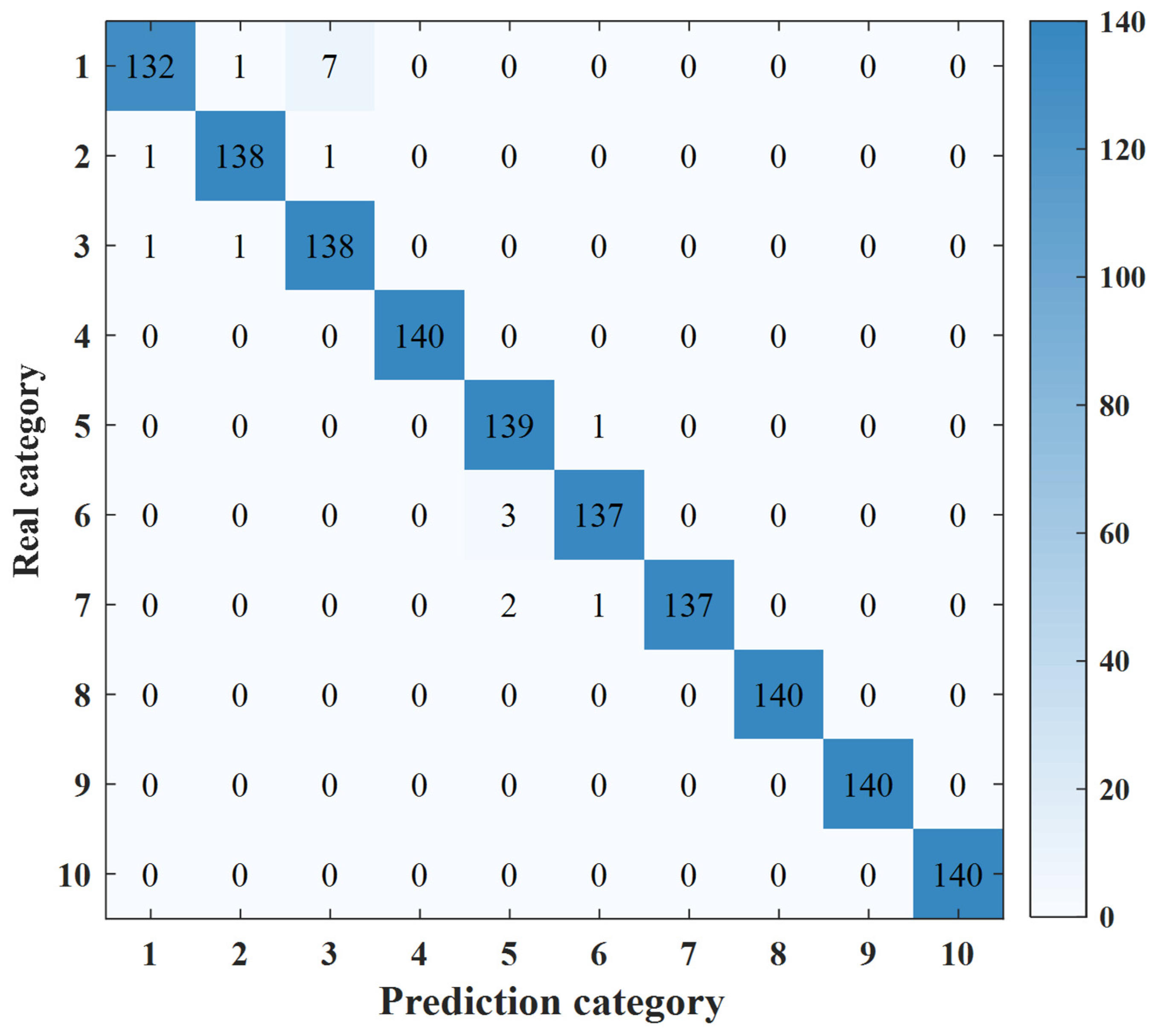
A confusion matrix-based multi class fault detection visualization was constructed to visually demonstrate the classification and detection capabilities of the FNKPCA–SVM detection model for different types of fault data, and graphical methods were used to reflect the classification performance of the detection module on different sample data classes (Figure 8).

An analysis of Figure 8 shows that the colors on the diagonal of the confusion matrix are generally darker, and the predicted fault labels correspond to the real fault labels (except for the classification labels of 3 and 5). This finding indicates that the FNKPCA–SVM detection model can effectively capture abnormal changes in various sensor data, ensuring the accuracy of fault prediction and improving the timeliness and reliability of fault warning.

In this study, the false alarm rate (FAR), missed detection rate (MDR), and recall rate (REC) are selected as the core evaluation indicators for module performance.

Table 4. Performance indicators under different types of faults.

Class	FAR	MDR	REC
1	0.16%	5.71%	94.29%
2	0.16%	1.43%	98.57%
3	0.63%	1.43%	98.57%
4	0%	0%	100%
5	0.40%	0.71%	99.29%
6	0.16%	2.14%	97.86%
7	0%	2.14%	97.86%
8	0%	0%	100%
9	0%	0%	100%
10	0%	0%	100%

presents the specific quantitative results under different fault types.

According to Table 4, the performance of the FNKPCA–SVM module in detecting Class 4, Class 8, and Class 10 faults is significantly better than that of other labels. For other types of label samples, the average recall rate of the module is as high as 98.22%. The stability and reliability of the experimental results of this study are ensured by independently repeating the experiments on the designed model 50 times. The results showed that the average prediction accuracy (ACC_ave) of the FNKPCA–SVM model can reach 98.64%.

The abovementioned results fully indicate that the designed fault detection module can accurately capture the characteristic changes in the navigation sensor fault data, demonstrating strong classification performance and greatly improving the accuracy of fault detection.

4.3. Active Fault-Tolerant Comparison Analysis

To comprehensively evaluate the effectiveness and robustness of the designed active fault-tolerant model for the UAV flight control system in the presence of navigation sensor faults, this section conducts a deeper comparative experiment on different fault-tolerant methods from the perspectives of various navigation sensors and fault factors.

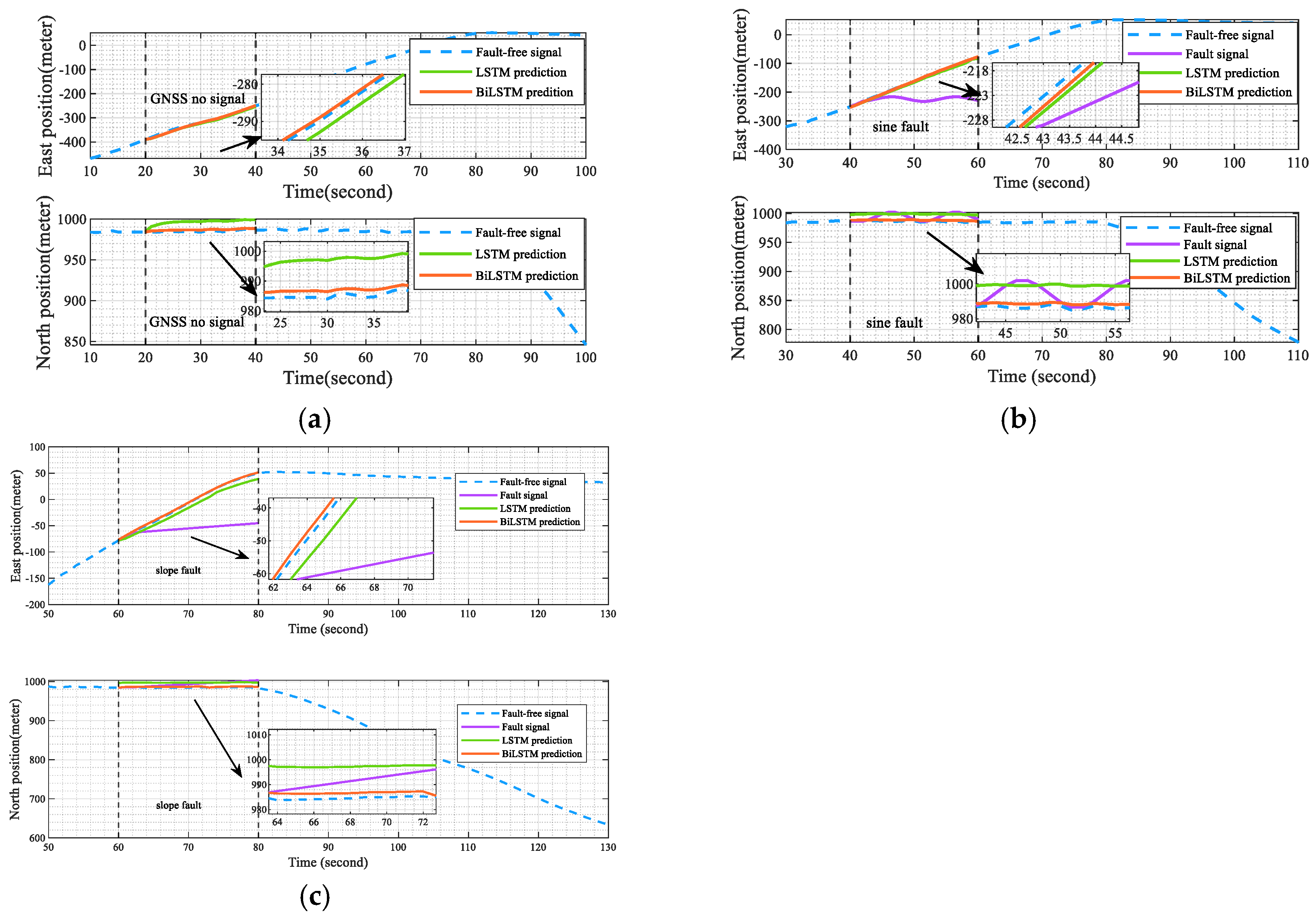
The GPS sensor is assumed to set a sudden fault generation interval between 20 s and 40 s in the east (x-axis) and north (y-axis) directions. After that, a sine fault occurred in both directions at 40 s, which lasted for a period of time before being repaired at 60 s, and the sensor continued to operate. At 60 s, a slope fault occurred in both directions, which disappeared at 80 s. Figure 9 shows a comparison of the predicted output of the GPS sensor under different fault states.

When the detection system determines that a fault occurs in the GPS sensor’s x-axis and y-axis, the difference between the predicted output value of the BiLSTM at the fault location and the actual value is not significant (Figure 8). At this point, the output of the actual GPS sensor can be masked in the fault-tolerant switching module, and BiLSTM predicted values can be used to indirectly participate in system control by replacing the actual values. From this finding, the predicted values of the BiLSTM fault-tolerant model designed in this study can replace the fault output when the actual sensor fails, ensuring the safety of UAV flight.

In addition, compared with those of the LSTM model, the predicted results of the BiLSTM fault-tolerant model are closer to the original normal data (blue dashed line) of the sensor during the fault period. This finding further demonstrates that the FNKPCA–SVM–BiLSTM active fault-tolerant method can better ensure the timely and effective functioning of the fault-tolerant approach.

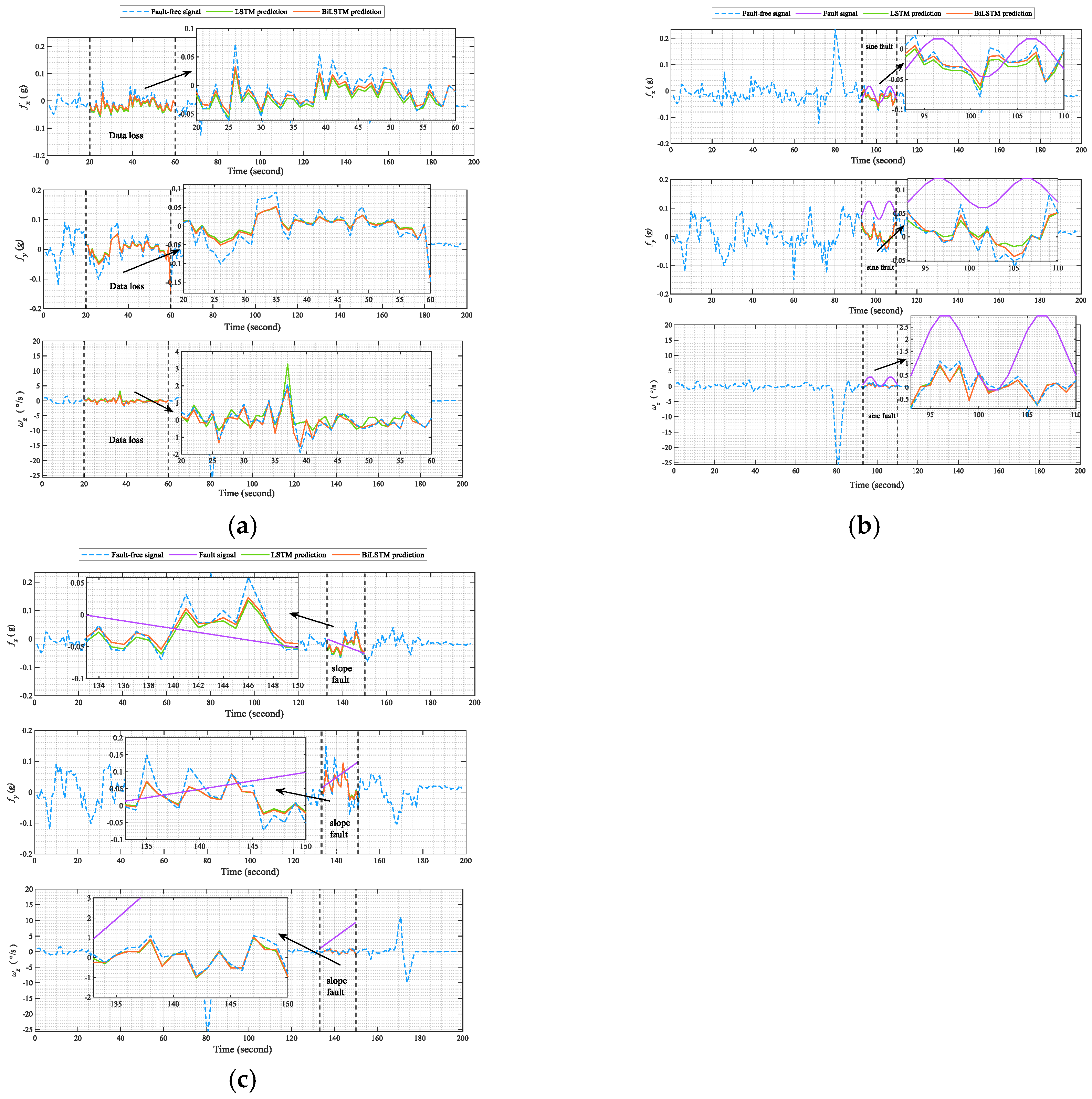
Considering that the flight attitude information of UAV mainly relies on the acceleration and angular velocity output by IMU and to ensure fairness and generalization in performance evaluation, the positions of sudden fault, sine fault, and slope fault introduced in the x-axis of IMU are selected as the time intervals of 20 s to 60 s, 93 s to 110 s, and 133 s to 150 s, respectively. Similarly, the fault status and duration on the y-axis and z-axis are consistent with those on the x-axis, ensuring the effectiveness of the analysis. Figure 10 shows the predictive output performance of IMU under different fault states.

Under the condition of introducing a fault in the x-axis of the IMU sensor, both the BiLSTM fault-tolerant model and the LSTM model have shown a certain predictive ability, but the output value predicted by the BiLSTM model is closer to the normal output of the sensor (Figure 10). This finding proves that in the event of a fault, the predicted results using the BiLSTM model can better reflect the attitude of the UAV system relative to the Earth and can replace the output signals of the faulty sensors to ensure the normal flight of the UAV. At the same time, when the fault state cycle changes or the fault change rate continues to increase, the predicted results of the sensor’s angular velocity under the BiLSTM fault-tolerant model and the LSTM model are almost identical, indicating that these two fault-tolerant models have similar sensitivity in discovering the potential characteristics of IMU sensor angular velocity and attitude drift.

Overall, the BiLSTM fault-tolerant model can more effectively capture the bidirectional dependencies of time series data, provide better predictive values, and reduce the adverse effects of faults on UAV system performance.

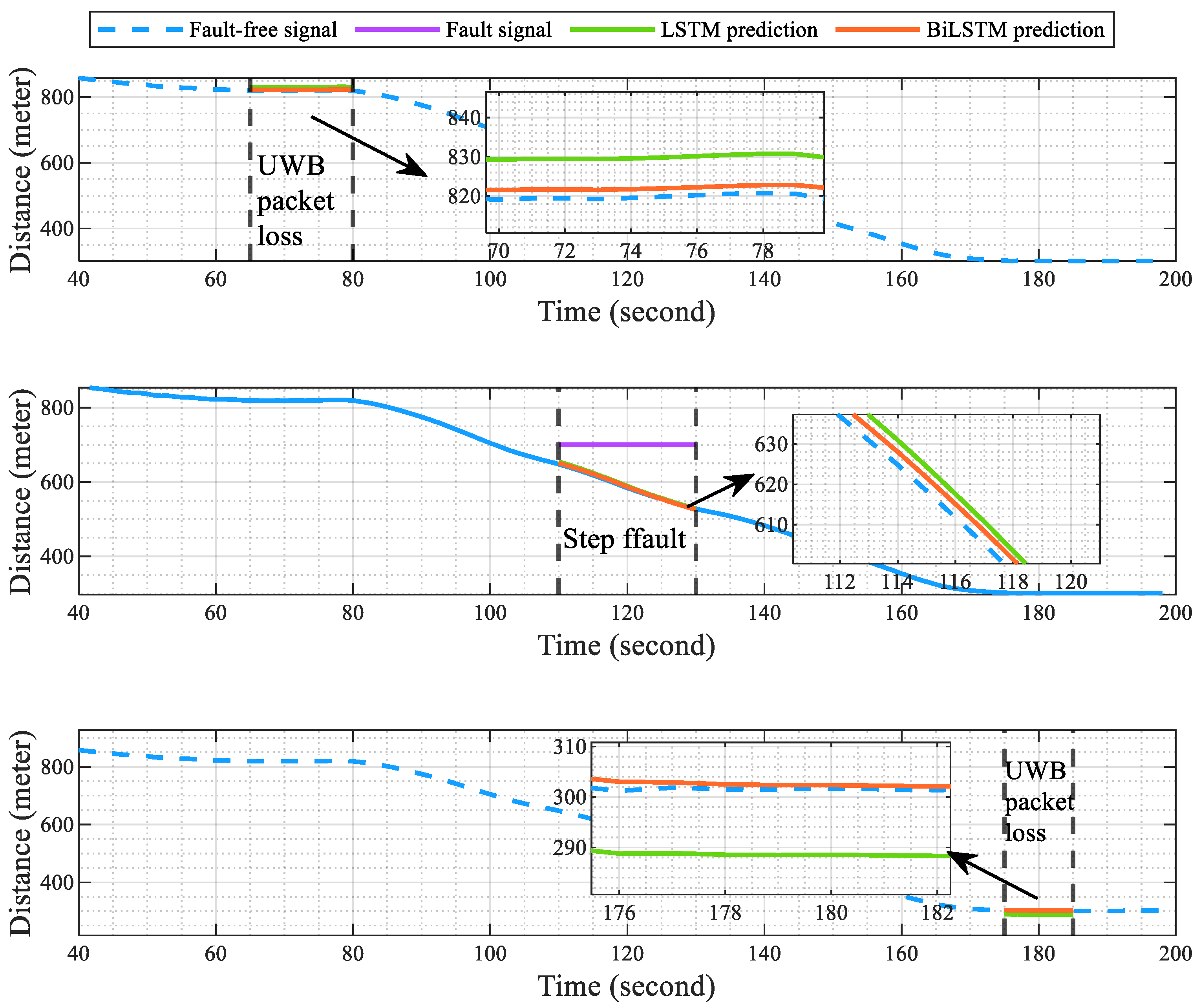
Three time periods with different distance change rates are considered to be selected to verify the adaptability of the fault-tolerant model to the output distance fault information of UWB sensors. Among them, the time intervals from 65 s to 80 s and from 175 s to 185 s represent periods of smooth distance change, which can be simulated by the UWB packet loss method to achieve sudden fault effects. The 110th to 130th seconds are the time period for rapid distance changes, and the effect of sudden faults is simulated by setting step values. Figure 11 shows the predictive performance of UWB under sudden fault.

The analysis of the above figure shows that the predicted results of the BiLSTM active fault-tolerant model (orange line) are closer to the normal output of the sensor (blue dashed line) compared with LSTM (green line) during the three fault time periods. Although the overall trend of LSTM’s predictions also aligns with the normal output of the sensor (blue dashed line), a certain degree of discrepancy exists.

4.4. Ablation Comparison Experiments

To clarify the advantages of the FNKPCA–SVM–BiLSTM model in structural design, this section presents an ablation discussion.

4.4.1. Comparison of Ablation Models for Fault Detection

To validate the structural rationale of the proposed FNKPCA–SVM fault detection model, three ablation experiments were conducted by modifying specific components of the original architecture. The first model, FNKPCA–RF, keeps the original network architecture but replaces the classifier with Random Forest (RF) [26,29], while the feature processing module still adopts FNKPCA. The second model, FNKPCA–DT, employs a Decision Tree (DT) as the classifier [26,30], while the rest of the structure is consistent with the original model. The third model, KPCA–SVM, is based on the original architecture but replaces the feature processing module with the traditional KPCA. The superiority of the original model structure is verified by comparing these three ablation models with the original FNKPCA–SVM model. All ablation models are trained on the same dataset and use the same parameter settings as the original FNKPCA–SVM model.

To ensure the reliability of the experimental results, comparative experiments are conducted 50 times for each model (FNKPCA–SVM, FNKPCA–DT, and FNKPCA–RF), and four indicators are recorded and analyzed: average n Accuracy (ACC_ave), average False Alarm Rate (FAR_ave), average Missed Detection Rate (MDR_ave), and average prediction Time (Time_ave).

Table 5. Performance result comparison between FNKPCA–SVM and other models.

Model	ACC_ave	FAR_ave	MDR_ave	Time_ave
FNKPCA–RF	98.50%	0.16%	1.50%	0.1368 s
FNKPCA–DT	98.43%	0.18%	1.57%	0.0801 s
KPCA–SVM	96.24%	0.42%	3.76%	0.4550 s
FNKPCA–SVM	98.64%	0.15%	1.16%	0.0403 s

provides the average performance results of all the models tested on a test dataset during the experimental process.

Based on the comparative data (Table 5), under the same dataset, the FNKPCA–SVM–based fault detection fusion method demonstrates significant comprehensive advantages in UAV navigation sensor fault detection tasks. Its average accuracy (ACC_ave) reaches 98.64%, outperforming other comparative models such as FNKPCA–RF (98.50%), FNKPCA–DT (98.43%), and KPCA–SVM (96.24%). These values highlight the FNKPCA–SVM module’s precise capability in identifying faults in UAV navigation sensors. Regarding error metrics, FNKPCA–SVM achieves the lowest values in both the average false alarm rate (FAR_ave = 0.15%) and the average missed detection rate (MDR_ave = 1.16%) in the table, outperforming the control models such as KPCA–SVM (FAR_ave = 0.42%, MDR_ave = 3.76%). These findings indicate the model’s high reliability during fault identification, effectively reducing the risks of misjudgment and missed detection. In terms of computational efficiency, the module’s average computation time (Time_ave = 0.0403 s) is substantially lower than that of KPCA–SVM (0.4550 s) and FNKPCA–RF (0.1368 s). This finding demonstrates the model’s ability to meet the low-latency requirements for UAV sensor fault detection while ensuring high precision, exhibiting superior adaptability for practical deployment.

This result indicates that by leveraging SVM to handle the dependencies between the time series of fault signal features, it not only ensures timely detection of fault signals but also effectively improves computational efficiency. The FNKPCA–SVM module has greater fault detection performance in navigation sensor fault prediction tasks, with higher accuracy and stronger computational capability, despite not using feature extraction methods as the input.

4.4.2. Comparison of Ablation Models for Fault Tolerance

The effectiveness of the BiLSTM active fault-tolerant model designed in this study is quantitatively analyzed by comparing it with the traditional LSTM model via the method called multi-index quantitative comparison.

Table 6. Comparison of Error Indicators between LSTM and BiLSTM Fault-Tolerant Models.

Sensor	Measurement Information	RMSE		MAE		PCC
		LSTM	BiLSTM	LSTM	BiLSTM	LSTM	BiLSTM
GPS	position m	9.632	2.140	8.650	1.830	1.000	1.000
IMU	acceleration g	0.021	0.018	0.015	0.013	0.905	0.953
	angular velocity °/s	0.367	0.263	0.249	0.184	0.817	0.916
UWB	distance m	9.078	2.242	8.185	2.018	0.990	1.000

shows a comparison of the RMSE, MAE, and Pearson Correlation Coefficient (PCC) indicators in the data processing results of the GPS, IMU, and UWB navigation sensors. The performance differences in fault-tolerant accuracy between the BiLSTM and LSTM models are intuitively presented to clarify the advantages of the BiLSTM model.

The calculation formulas for the RMSE, MAE, and PCC are as follows [26,31]:

$$RMSE=\sqrt{{\displaystyle \frac{1}{N}}{\sum }_{i=1}^N{\left(y_{pred,i}-y_{actual,i}\right)}^2},$$

(10)

$$MAE={\displaystyle \frac{1}{N}}{\sum }_{i=1}^N\left|y_{pred,i}-y_{actual,i}\right|,$$

(11)

$$PCC={\displaystyle \frac{{\sum }_{i=1}^N\left(y_{pred,i}-{\overline{y}}_{pred}\right)\left(y_{actual,i}-{\overline{y}}_{actual}\right)}{\sqrt{{\sum }_{i=1}^N{\left(y_{pred,i}-{\overline{y}}_{pred}\right)}^2}·\sqrt{{\sum }_{i=1}^N{\left(y_{actual,i}-{\overline{y}}_{actual}\right)}^2}}},$$

(12)

where N denotes the number of samples, y_pred,i represents the predicted value of the i-th sample, y_actual,i denotes the actual value of the i-th sample, ${\overline{y}}_{pred}$ indicates the average value of the predicted values, ${\overline{y}}_{actual}$ denotes the average value of the actual observed values, and ${\sum }_{i=1}^N$ refers to the summation over all N samples.

The predictive performance of the BiLSTM model is significantly better than that of LSTM on various data, indicating its stronger fault tolerance (Table 6). The specific analysis is as follows:

First, from the performance indicators of the GPS, the BiLSTM model has significantly lower RMSE (2.140 m) and MAE (1.83 m) compared with the LSTM model (RMSE = 9.632 m, MAE = 8.650 m), with error reductions of 77.8% and 78.8%, respectively. This finding indicates that the BiLSTM model improves prediction accuracy through bidirectional time series feature modeling, effectively avoiding the accuracy decline issue caused by the unidirectional time series processing in the LSTM model. In addition, the PCC value of BiLSTM and LSTM both reached 1.000, indicating a very strong linear correlation between the GPS prediction results and the actual values for both models. This result also demonstrates that time series neural network models have strong learning and modeling capabilities for sequential sensor data.

Second, for IMU, the RMSE (0.018 g) and MAE (0.013 g) of BiLSTM in acceleration prediction are lower than those of LSTM (RMSE = 0.021 g, MAE = 0.015 g), with error reductions of 14.3% and 13.3%, respectively, and the PCC value reaches 0.953. These results reflect that BiLSTM can more accurately capture the temporal correlation of acceleration signals. In angular velocity prediction, the RMSE (0.263 °/s) and MAE (0.184 °/s) of BiLSTM are both lower than those of LSTM (RMSE = 0.367 °/s, MAE = 0.249 °/s), and the PCC value (0.9164) is closer to 1, indicating better overall performance

Finally, the indicators of UWB further validated the advantage of BiLSTM’s fault tolerance performance; the RMSE (2.242 m) and MAE (2.018 m) of its distance prediction values are both approximately 75% lower than those of LSTM (9.078 and 8.185 m). The PCC value of BiLSTM and LSTM are 0.99 and 1.00, respectively, indicating a strong linear correlation between the predicted results of both models and the true values.

In summary, time series neural networks can effectively extract time-series features and have a certain degree of fault tolerance when processing navigation sensor data. The BiLSTM neural network model demonstrates higher accuracy in dealing with faults due to its bidirectional time series modeling capability.

5. Discussion

This study addresses the challenge of fault-tolerant control for unmanned aerial vehicles (UAVs) in complex dynamic environments and systematically evaluates the proposed FNKPCA–SVM–BiLSTM active fault-tolerant method. Integrating the F-norm with kernel principal component analysis (KPCA) allows this method to effectively suppress fault underreporting and misjudgment and ultimately improve system reliability and classification accuracy. Additionally, the introduction of the SVM classifier further enhances the model’s generalization ability for complex fault features. Experiments show that this method achieves excellent fault detection accuracy, significantly reducing the risk of UAV crashes and collisions caused by sensor abnormalities, thereby improving the safety and mission completion rate of UAV flights in complex environments. However, the method still has limitations. First, in environments with strong noise interference, the model’s ability to identify fault signals decreases, which may lead to an increase in the false alarm rate. Second, for small-sample rare fault types, due to insufficient samples, the classification accuracy fluctuates, and the model’s adaptability to such faults needs further improvement.

6. Conclusions

The safety and stability issues caused by faults in UAV navigation sensors are addressed by proposing an active fault-tolerant method based on FNKPCA–SVM–BiLSTM. The core contribution is the construction of a collaborative fault-tolerant architecture of “feature enhancement–classification discrimination–time series prediction.” Experimental results showed that this method achieves a detection accuracy of up to 98.64% for abnormal data of navigation sensors. The dual advantages of high detection accuracy and predictive advance can not only reduce invalid actions of the actuator but also achieve a balance between fault-tolerant performance and delay cost, providing theoretical and practical support for the engineering implementation of UAV active fault-tolerant methods. The following directions are recommended for future work to further enhance the robustness and adaptability of the proposed method:

• Multisensor collaborative fault-tolerant mechanism: For scenarios where GPS denial and IMU drift coexist, a multimodal feature fusion mechanism can be introduced to improve the distinguishability of fault features.
• Delay optimization mechanism: Focusing on the dynamic changes in actuator delay with flight phases, parameter adaptive methods can be explored to mitigate the impact of noise interference on delay under complex working conditions.
• Fault dataset construction: An annotated dataset with multiple scenarios and multiple fault types can be built, combining it with data augmentation technology to solve the problem of scarcity of measured fault samples.
• Field verification: Experiments in unstructured real environments can be conducted to verify the scalability and reliability of the algorithm in real scenarios.