A Novel Evaluation Method for Vibration Coupling of Complex Rotor–Stator Systems in Aeroengines

Abstract

With the increase in thrust–weight ratio of advanced aeroengines, the rotor and stator often exhibit comparable stiffness characteristics, leading to significant vibration coupling which harms the safety and reliability of operations. However, an effective vibration coupling evaluation method for complex rotor–stator systems is still lacking. This paper proposes the Vibration Coupling Evaluation Factor (VCEF) to quantitatively evaluate the interaction between the rotor and stator within the framework of the linear system. Then a new evaluation procedure is established for the structural optimization during the early design phase and the fault source localization in troubleshooting scenarios in the high-speed rotating machinery. In this paper, two typical rotor–stator systems are studied with the VCEF method: a simplified rotor–stator system is studied numerically to reveal the influence pattern of different parameters, and a complex rotor–stator system is studied numerically and experimentally to examine the validity of the evaluation method. The results show that VCEF can effectively capture rotor–stator vibration coupling. The VCEF curve with rotational speed shows a significant stepped decrease, indicating a significant strengthening of the rotor–stator vibration coupling, which aligns closely with experimental data. This evaluation method quantitatively assesses the degree of rotor–stator vibration coupling by comparing the differences in modal characteristics between the rotor system and the rotor–stator system under the gyroscopic effect. Optimizing rotor–stator stiffness and mass distribution based on VCEF mitigates operational risks in high-speed regimes. This methodology provides engineers with a systematic, quantitative tool to determine when integrated rotor–stator analysis is essential for accurate dynamic prediction and offers broad applicability to aeroengine design and other high-speed rotating machinery.

1. Introduction

The modern aeroengine, a pivotal component of aviation technology, operates under extreme conditions that demand precise dynamic analysis to ensure safety and performance [1,2,3,4,5]. A critical challenge in rotor dynamics is accurately predicting the system’s dynamic behavior, which has traditionally been analyzed by isolating the rotor subsystem. However, in contemporary aeroengines, the stator often exhibits stiffness characteristics comparable to those of the rotor [6,7,8], leading to significant rotor–stator vibration coupling, which will significantly alter the system’s dynamic response and potentially undermine the prediction accuracy of critical rotational speeds and imbalance responses [9,10]. These are vital for safe and efficient engine operation, driving recent research to extend beyond the rotor-only system towards the rotor–stator system, including bearing, supporting structure, and casing [11,12,13,14].

Previous studies have predominantly concentrated on the rotor-only system, neglecting the interaction between the rotor and stator [15,16,17,18]. This simplification introduces significant inaccuracies, particularly at the high operational speeds of modern aeroengines. Pioneering work by Cheli [6] highlighted the influence of the stator on rotor dynamic behavior, noting that when the natural frequency of the supporting structure approaches the rotor’s operational speed, the rotor–stator system’s dynamic response will be significantly altered. Subsequent studies have attempted to incorporate stator effects. Parent [19] introduced a fully-coupled phenomenological model with flexible blades, shaft, and casing to research the influence of the whole engine dynamic on contact-related behavior. Liu [20,21] established the finite element model of the rotor–stator system and studied the nonlinear dynamic behavior that may occur under the rotor-casing rubbing faults in aeroengines. However, the finite element model of the stator, constructed with beam elements, is unsuitable for accurately representing the large inner diameter and thin-walled casing typical of aeroengines. Zhou [22] proposed a 5-DOF model capturing strong vibration coupling between elastic supporting structures and bearings. Dai [23] proposed the modeling strategy for the dual-rotor-disc-bearing coupled system with an unbalance effect in aeroengines. Wang [24] highlighted significant rotor–stator vibration coupling under maneuver loads. Despite considerable efforts [25,26,27,28,29], prevailing models often rely on simplifying assumptions that fail to fully capture the complex dynamics of the interaction between the rotor and stator. Especially in high-speed rotating machinery, the rotor operates above multiple critical speeds, exhibiting significant flexibility, in which rotor–stator vibration coupling becomes pronounced and can dominate dynamic behavior [30,31].

In order to effectively evaluate the dynamic response of these complex systems, like the rotor–stator system, researchers have developed numerous modeling strategies. Hu [32] established a finite element model of rotor-supporting structure systems and verified the accuracy of the natural frequency, critical rotational speed, and logarithmic decrement. Dewi [33] determined the critical rotational speed and damping coefficient through the frequency response functions (FRF) of rotor-supporting structure systems. Chen [34] used the pseudo mode shape method (PMSM) to accurately identify the parameter matrix of the rotor-bearing-foundation structure. Katia [35,36] proposed a method to analyze the influence of the supporting structure on the rotor-bearing system by considering physical coordinates for the rotor-bearings system and principal coordinates for the support. Bonello [37,38] used the receptance harmonic balance technique and impulsive receptance technique to calculate the response of the rotor-casing system, and obtained the dynamic behavior of the whole aeroengine system with nonlinear bearings.

After modeling and dynamic analysis of complex systems, interpreting the results to extract relevant insights constitutes an essential subsequent step. In most cases, direct dynamic response outputs, such as displacements and velocities, provide a simple evaluation but lack an effective evaluation of the entire system [24,39]. Petrone [40,41] evaluated vibration behavior in the medium–high frequency range of an aircraft fuselage section by using the Statistical Energy Analysis (SEA) method. Kim [42,43] employed transmissibility functions to compensate for disturbances due to base excitation and to estimate, based on the transfer path analysis, the operational force of the main vibration source in a complicated system. Ma [44,45] investigated energy flow transmission in rotor systems using the structural intensity method. In parallel, because of the simplicity and robustness, the Modal Assurance Criterion (MAC) has become a fundamental tool in structural dynamics for model validation, such as studying rotor–stator contact dynamics [46], detecting subsystem interactions [47,48], and so on. However, the above methods are not suitable for the rotor–stator systems in aeroengines, primarily due to insufficient consideration of the gyroscopic effect. Rotor–stator vibration coupling would vary with rotational speed and is not universally dominant across all systems or operating conditions [49,50]. Consequently, there is a compelling need for a robust quantitative evaluation method to assess rotor–stator vibration coupling.

To address this gap, this study introduces a novel quantitative evaluation method for rotor–stator vibration coupling, and the Vibration Coupling Evaluation Factor (VCEF) is proposed to quantify the similarity between the dynamic characteristics of the rotor-only system and the rotor–stator system versus rotational speeds. This method focuses on the linear system, delivers structural optimization guidance during the early design phase, and enables precise fault root cause identification in troubleshooting scenarios.

The remainder of this paper is organized as follows: Section 2 derives the theoretical model and details the VCEF methodology. Section 3 presents numerical simulation results of a simplified rotor–stator system, illustrating dynamic behavior under various conditions and parameter sensitivities. Section 4 presents numerical simulation results of a complex rotor–stator system, and Section 5 conducts the experimental validation. Section 6 summarizes the key conclusions.

2. Evaluation Method of Rotor–Stator Vibration Coupling

This section focuses on the rotor–stator system of aeroengines as the research object. The motion equations are derived, and the Vibration Coupling Evaluation Factor (VCEF) is proposed, providing a quantitative evaluation of rotor–stator vibration coupling.

2.1. Motion Equation

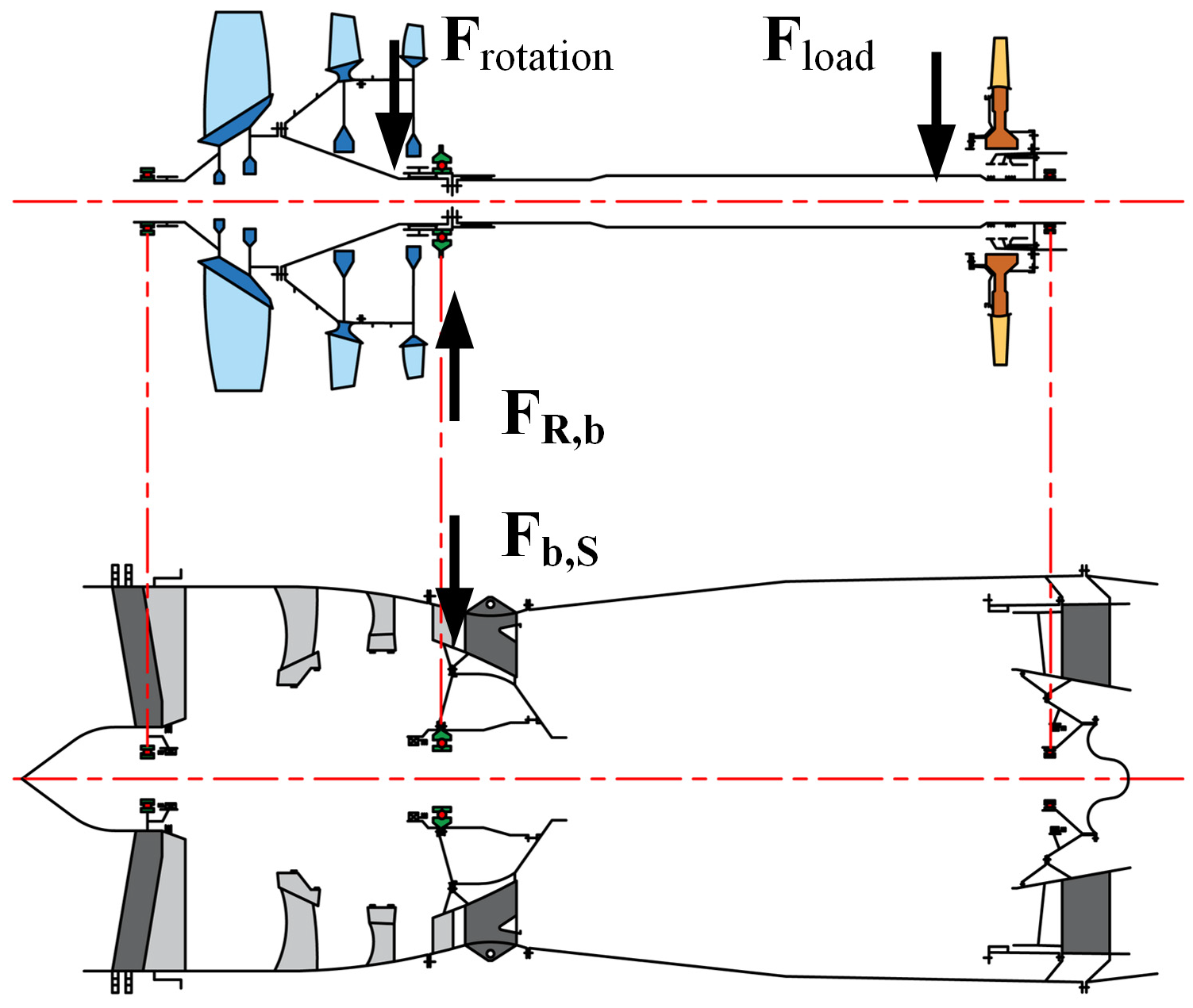
During rotation, the rotor is subjected to the unbalanced load $F_{rotation}$ and other dynamic force $F_{load}$, resulting in dynamic response, a common phenomenon in rotating machinery. Figure 1 presents the abstract expression of the rotor–stator in the aeroengine: an unbalanced rotor operates in the bearings mounted on a flexible stator. The stator provides insufficient constraint on the rotor and bearings, leading to interactions between the stator and bearings that significantly influence the system’s dynamic behavior. These interactions result in rotor–stator vibration coupling.

Therefore, the Lagrange equation is used to derive the motion equation of the rotor–stator system:

$${\displaystyle \frac{d}{dt}}\left({\displaystyle \frac{\partial T}{\partial {\dot{\mathit{q}}}_{\mathit{i}}}}\right)-{\displaystyle \frac{\partial T}{\partial {\mathit{q}}_{\mathit{i}}}}+{\displaystyle \frac{\partial V}{\partial {\mathit{q}}_{\mathit{i}}}}+{\displaystyle \frac{\partial D}{\partial {\dot{\mathit{q}}}_{\mathit{i}}}}={\mathit{F}}_{\mathit{i}}$$

(1)

where $T$, $V$, and $D$ are, respectively, kinetic energy, potential energy, and dissipated energy, and ${\mathit{F}}_{\mathit{i}}$ is the external force. ${\mathit{q}}_{\mathit{i}}$ represents the degree of freedom (DOF) vector of one node at a generalized coordinate:

$${\mathit{q}}_{\mathit{i}}={\left[\begin{array}{cccc}{x}_i& y_i& {\theta }_{x,i}& {\theta }_{y,i}\end{array}\right]}^T$$

(2)

Assume that the rotor–stator system consists of R + S nodes, where the rotor has R nodes and the stator has S nodes. Thus, the generalized coordinates can be expressed as follows:

$${\mathit{q}}_{\mathit{r}}={\left\{\begin{array}{cccc}{\mathit{q}}_1& {\mathit{q}}_2& \cdots & {\mathit{q}}_R\end{array}\right\}}^T$$

(3)

$${\mathit{q}}_{\mathit{s}}={\left\{\begin{array}{cccc}{\mathit{q}}_{R+1}& {\mathit{q}}_{R+2}& \cdots & {\mathit{q}}_{R+S}\end{array}\right\}}^T$$

(4)

$${\mathit{q}}_{\mathit{w}}={\left\{\begin{array}{cc}{\mathit{q}}_{\mathit{r}}& {\mathit{q}}_{\mathit{s}}\end{array}\right\}}^T={\left\{\begin{array}{cccccc}{\mathit{q}}_1& \cdots & {\mathit{q}}_R& {\mathit{q}}_{R+1}& \cdots & {\mathit{q}}_{R+S}\end{array}\right\}}^T$$

(5)

where ${\mathit{q}}_{\mathit{r}}$ and ${\mathit{q}}_{\mathit{s}}$ represent the rotor and stator coordinates, and ${\mathit{q}}_{\mathit{w}}$ represents the rotor–stator coordinates.

The motion equation of the rotor system and the rotor–stator system are, respectively, as follows:

$${\mathit{M}}_{\mathit{r}}{\ddot{\mathit{q}}}_{\mathit{r}}+\left({\mathit{C}}_{\mathit{r}}+{\mathit{G}}_{\mathit{r}}\right){\dot{\mathit{q}}}_{\mathit{r}}+{\mathit{K}}_{\mathit{r}}{\mathit{q}}_{\mathit{r}}={\mathit{F}}_{\mathit{r}}$$

(6)

$${\mathit{M}}_{\mathit{w}}{\ddot{\mathit{q}}}_{\mathit{w}}+\left({\mathit{C}}_{\mathit{w}}+{\mathit{G}}_{\mathit{w}}\right){\dot{\mathit{q}}}_{\mathit{w}}+{\mathit{K}}_{\mathit{w}}{\mathit{q}}_{\mathit{w}}={\mathit{F}}_{\mathit{w}}$$

(7)

where ${\mathit{M}}_{\mathit{r}}$, ${\mathit{C}}_{\mathit{r}}$, ${\mathit{G}}_{\mathit{r}}$, and ${\mathit{K}}_{\mathit{r}}$ represent the mass, damping, gyroscopic, and stiffness matrices of the rotor system, and ${\mathit{M}}_{\mathit{w}}$, ${\mathit{C}}_{\mathit{w}}$, ${\mathit{G}}_{\mathit{w}}$, and ${\mathit{K}}_{\mathit{w}}$ represent the mass, damping, gyroscopic, and stiffness matrices of the rotor–stator system. ${\mathit{F}}_{\mathit{r}}$ and ${\mathit{F}}_{\mathit{w}}$ represent the external forces acting on the rotor system and the rotor–stator system. And the equation of motion in Equation (7) can be presented:

$$\left[\begin{array}{cc}{\mathit{M}}_{\mathit{r}}& 0\\ 0& {\mathit{M}}_{\mathit{s}}\end{array}\right]\left\{\begin{array}{c}{\ddot{\mathit{q}}}_{\mathit{r}}\\ {\ddot{\mathit{q}}}_{\mathit{s}}\end{array}\right\}+\left(\left[\begin{array}{cc}{\mathit{C}}_{\mathit{r}}& 0\\ 0& {\mathit{C}}_{\mathit{s}}\end{array}\right]+\left[\begin{array}{cc}{\mathit{G}}_{\mathit{r}}& 0\\ 0& 0\end{array}\right]\right)\left\{\begin{array}{c}{\dot{\mathit{q}}}_{\mathit{r}}\\ {\dot{\mathit{q}}}_{\mathit{s}}\end{array}\right\}+\left[\begin{array}{cc}{\mathit{K}}_{\mathit{r}\mathit{r}}& {\mathit{K}}_{\mathit{r}\mathit{s}}\\ {\mathit{K}}_{\mathit{s}\mathit{r}}& {\mathit{K}}_{\mathit{s}\mathit{s}}\end{array}\right]\left\{\begin{array}{c}{\mathit{q}}_{\mathit{r}}\\ {\mathit{q}}_{\mathit{s}}\end{array}\right\}=\left\{\begin{array}{c}{\mathit{F}}_{\mathit{r}}\\ 0\end{array}\right\}$$

(8)

where ${\mathit{M}}_{\mathit{s}}$ and ${\mathit{C}}_{\mathit{s}}$ represent the mass and damping matrices of the stator. ${\mathit{K}}_{\mathit{r}\mathit{r}}$ and ${\mathit{K}}_{\mathit{s}\mathit{s}}$ represent the stiffness submatrices of the rotor and stator component in the rotor–stator system.

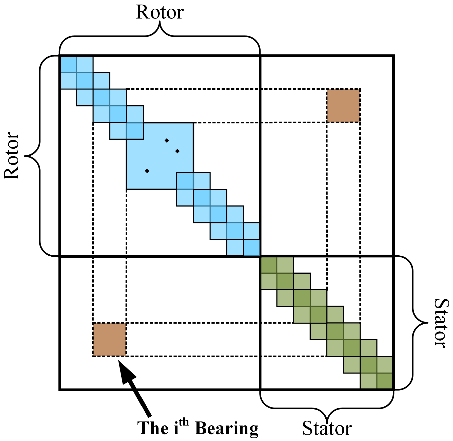
In rotor–stator systems, there is an interaction between the rotor and stator which results in vibration coupling. The rotor’s motion can excite the stator, and vice versa, altering their individual dynamic responses. The matrices ${\mathit{K}}_{\mathit{r}\mathit{s}}$ and ${\mathit{K}}_{\mathit{s}\mathit{r}}$ are the off-diagonal submatrices of the stiffness matrix ${\mathit{K}}_{\mathit{w}}$, as shown in Figure 2.

It can be seen from Figure 2 that that the rotor submatrix ${\mathit{K}}_{\mathit{r}\mathit{r}}$ and the stator submatrix ${\mathit{K}}_{\mathit{s}\mathit{s}}$ retain the original structural parameters. The off-diagonal submatrices ${\mathit{K}}_{\mathit{r}\mathit{s}}$ and ${\mathit{K}}_{\mathit{s}\mathit{r}}$ mathematically explain the mechanism of rotor–stator vibration coupling. These additional terms in the motion equations represent the interaction between the rotor and stator, which significantly affects the dynamic behavior of the system, particularly at higher rotational speeds.

2.2. The Vibration Coupling Evaluation Factor

To assess the degree of rotor–stator vibration coupling, the Vibration Coupling Evaluation Factor (VCEF) has been introduced to quantify the similarity between the mode shapes of the rotor-only system and the rotor–stator system.

The external force is assumed to have a harmonic form:

$$\mathit{F}(t)={\mathit{F}}_0\sin \omega t$$

(9)

Thus, based on the concept of mode shape superposition, the motion equation for the i-th normal coordinate can be written as follows:

$$m_i{\ddot{\mathit{\delta }}}_i(t)+c_i{\dot{\mathit{\delta }}}_i(t)+k_i{\mathit{\delta }}_i(t)={\mathit{N}}_{0i}{e}^{j\omega t}(i=1,2,\dots ,n)$$

(10)

where ${\mathit{N}}_{0i}={\mathit{u}}^{(i)\mathrm{{\rm T}}}{\mathit{F}}_0$ represents the external force for the i-th normal coordinate. Here, ${\mathit{u}}^{(i)}(i=1,2,\dots ,n)$ is the eigenvalue solution of Equation (10), namely the mode shape vector.

The steady-state response in the normal coordinates can be expressed as follows:

$${\mathit{\delta }}_i(t)={\mathbf{\Delta }}_{0i}\left|H_i(\omega )\right|e^{j(\omega t-{\phi }_i)}$$

(11)

where ${\mathbf{\Delta }}_{0i}={\mathit{N}}_{0i}/k_i$ represents the zero-frequency deflection in the normal coordinates. Here, $\left|H_i(\omega )\right|$, ${\phi }_i$, and ${\lambda }_i$ correspond to the amplification factor, phase angle, and frequency ratio in the normal coordinates, respectively:

$$\left|H_i(\omega )\right|={\displaystyle \frac{1}{\sqrt{{(1-{\lambda }_i^2)}^2+{(2{\xi }_i{\lambda }_i)}^2}}}$$

(12)

$$\begin{array}{cc}{\phi }_i=\arctan {\displaystyle \frac{2{\xi }_i{\lambda }_i}{1-{\lambda }_i^2}}& {\lambda }_i=\omega /{\omega }_{n,i}\end{array}$$

(13)

where ${\omega }_{n,i}$ is the i-th natural frequency.

Therefore, the steady-state response in the original physical space coordinates can be expressed as follows:

$$\mathit{q}(t)={\displaystyle \sum _{i=1}^n{\mathit{u}}^{(i)\mathrm{{\rm T}}}{\mathit{\delta }}_i(t)}={\displaystyle \sum _{i=1}^n{\mathit{u}}^{(i)\mathrm{{\rm T}}}{\mathbf{\Delta }}_{0i}\left|H_i(\omega )\right|\sin (\omega t-{\phi }_i)}$$

(14)

Under different loading conditions, ${\mathbf{\Delta }}_{0i}$ and ${\phi }_i$ with different DOFs vary accordingly. However, for a given system, ${\mathit{u}}^{(i)}$ and $H_i(\omega )$ in Equation (14) remain invariant with respect to loading conditions. The objective of this evaluation method is to assess the similarity of the modal characteristics of the rotor–stator system as a function of rotational speed. To minimize the influence of the form and magnitude of load vector $\mathit{F}(t)$ on the response characteristics, it is assumed that ${\mathbf{\Delta }}_{0r}=1(i=1,2,\dots ,n)$ in this study, and the phase difference ${\phi }_i$ between different modal frequencies is neglected. As a result, the dynamic response of the system can be expressed as follows:

$$\mathit{q}(t)=\left({\displaystyle \sum _{i=1}^n{\mathit{u}}^{(i)}\left|H_i(\omega )\right|}\right)\sin (\omega t)=\left({\mathit{u}}^{\mathrm{{\rm T}}}\cdot \left|\mathit{H}(\omega )\right|\right)\sin (\omega t)$$

(15)

For the multiple-degree-of-freedom system, a given mode order $N$ is typically selected during analysis. Only the selected mode shape vectors will be considered, and others will be truncated. Under a reasonable mode selection, an ideal analysis result can be obtained in engineering applications.

The i-th mode shape vectors of the rotor system and the rotor–stator system can be, respectively, expressed as follows:

$${\mathit{u}}_{\mathit{r}}^{(i)}={\left\{\begin{array}{cccc}{\mathit{u}}_1^{(i)}& {\mathit{u}}_2^{(i)}& \cdots & {\mathit{u}}_R^{(i)}\end{array}\right\}}^T$$

(16)

$${\mathit{u}}_{\mathit{W}}^{(i)}={\left\{\begin{array}{cc}{\mathit{u}}_w^{(i)}& {\mathit{u}}_s^{(i)}\end{array}\right\}}^T={\left\{\begin{array}{cccccc}{\mathit{u}}_1^{(i)}& \cdots & {\mathit{u}}_R^{(i)}& {\mathit{u}}_{R+1}^{(i)}& \cdots & {\mathit{u}}_{R+S}^{(i)}\end{array}\right\}}^T$$

(17)

where ${\mathit{u}}_w^{(i)}$ and ${\mathit{u}}_s^{(i)}$ represent the i-th mode shape vectors of the rotor component and stator component within the rotor–stator system. ${\mathit{u}}_{\mathit{r}}^{(i)}$ and ${\mathit{u}}_w^{(i)}$ are both the vectors of $R\times 1$.

For the rotor–stator system of aeroengines, the dynamic responses of the rotor system and the rotor component within the rotor–stator system can be, respectively, expressed as follows:

$${\mathit{q}}_r(t)={\mathit{u}}_r\cdot {\mathit{\delta }}_r(t)={\displaystyle \sum _{i=1}^N{\mathit{u}}_r^{(i)\mathrm{T}}\left|H_i(\omega )\right|e^{j(\omega t-{\phi }_i)}}={\displaystyle \sum _{i=1}^N{\mathit{Q}}_r^{\left(i\right)}{e}^{j(\omega t-{\phi }_i)}}$$

(18)

$${\mathit{q}}_w(t)={\mathit{u}}_w\cdot {\mathit{\delta }}_w(t)={\displaystyle \sum _{i=1}^N{\mathit{u}}_w^{(i)\mathrm{T}}\left|H_i(\omega )\right|e^{j(\omega t-{\phi }_i)}}={\displaystyle \sum _{i=1}^N{\mathit{Q}}_w^{\left(i\right)}{e}^{j(\omega t-{\phi }_i)}}$$

(19)

The response amplitude vectors corresponding to the mode orders of the two components can be expressed as follows:

$${\mathit{Q}}_{\mathit{r}}={{\mathit{u}}_r}^{\mathrm{{\rm T}}}\left|\mathit{H}(\omega )\right|={\left[\begin{array}{c}{\mathit{u}}_r^{(1)}\\ {\mathit{u}}_r^{(2)}\\ ⋮\\ {\mathit{u}}_r^{(N)}\end{array}\right]}^{\mathrm{{\rm T}}}\times \left[\begin{array}{c}{H}_1(\omega )\\ H_2(\omega )\\ ⋮\\ H_N(\omega )\end{array}\right]$$

(20)

$${\mathit{Q}}_{\mathit{w}}={{\mathit{u}}_w}^{\mathrm{{\rm T}}}\left|\mathit{H}(\omega )\right|={\left[\begin{array}{c}{\mathit{u}}_w^{(1)}\\ {\mathit{u}}_w^{(2)}\\ ⋮\\ {\mathit{u}}_w^{(N)}\end{array}\right]}^{\mathrm{{\rm T}}}\times \left[\begin{array}{c}{H}_1(\omega )\\ H_2(\omega )\\ ⋮\\ H_N(\omega )\end{array}\right]$$

(21)

From Equations (18) and (19), it is evident that the response differences between the two systems are primarily concentrated in the variations of their respective mode shape vectors. Regarding ${\mathit{u}}_r$ and ${\mathit{u}}_w$, the similarity of the two mode shape vectors can be quantitatively characterized with the Mode Shape Correlation Coefficient (MSCC). The MSCC [51,52,53,54,55,56,57], also known as the Modal Assurance Criterion (MAC), a well-established statistical indicator highly sensitive to the mode shape differences, provides a reliable measure of consistency between mode shape vectors. And it can be expressed as follows:

$$MSCC(\omega ,i,j)={\displaystyle \frac{{\left[{\mathit{u}}_w^{(i)\mathrm{H}}{\mathit{u}}_r^{(j)}\right]}^2}{\left|{\mathit{u}}_w^{(i)}\right|\cdot \left|{\mathit{u}}_r^{(j)}\right|}}$$

(22)

The $MSCC(\omega ,i,j)$ represents the similarity of the i-th mode shape vector of the rotor component within the rotor–stator system and the j-th mode shape vector of the rotor system at the rotational speed $\omega$. The MSCC value ranges from 0 to 1, with 1 indicating perfect similarity and 0 indicating no similarity.

The MSCCs can be calculated for each mode based on Equation (22), and the MSCC distribution at a specific rotational speed allows for the identification of rotor-dominated modes—the modes where rotor deformation significantly influences the system’s dynamic response in Equations (20) and (21).

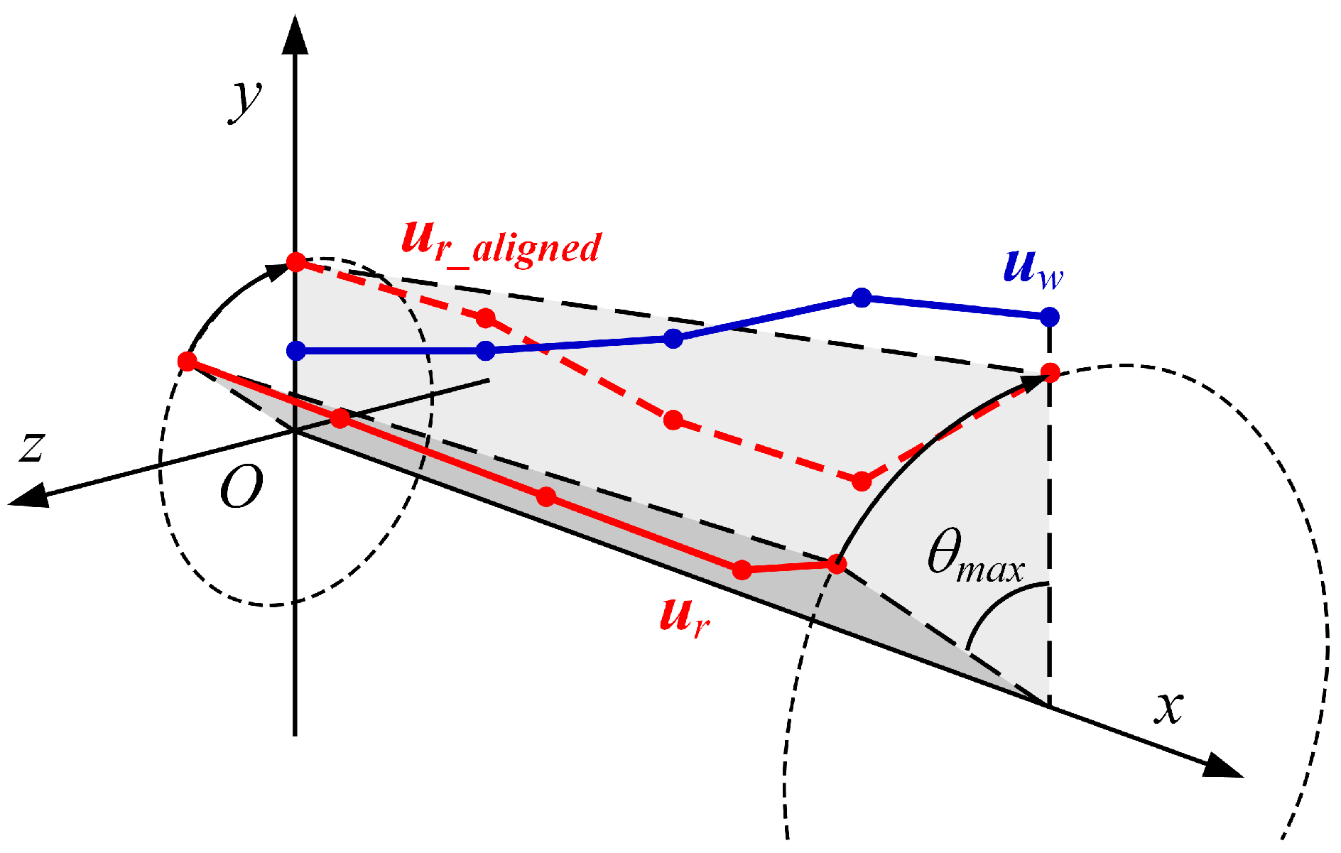
It should be noted that there may be a potential impact on the MSCC because of the phase misalignment of the mode shape vector. Usually, the vector rotation is involved to realign phase angles, eliminating correlation errors:

$$\begin{array}{cc}{\mathit{u}}_{r\_aligned}^{(i)}={\mathit{u}}_r^{(i)}\cdot \exp \left(-j{\theta }_{\max }\right)& {\theta }_{\max },s.t.\min {\displaystyle \sum _{i=1}^n{\left[{\mathit{u}}_w^{(i)}(i)-\left({\mathit{u}}_r^{(i)}(i)\cdot \exp \left(-j{\theta }_{\max }\right)\right)\right]}^2}\end{array}$$

(23)

The mode shape vectors ${\mathit{u}}_r$ and ${\mathit{u}}_w$ can be projected in a common global coordinate system to eliminate the phase misalignment artifacts, as shown in Figure 3, which ensures MSCC solely quantifies shape correlation rather than coordinate differences. In subsequent sections, ${\mathit{u}}_r$ denotes ${\mathit{u}}_{r\_aligned}$ for brevity.

For the rotor-dominated modes, there is a one-to-one correspondence between the rotor system and the rotor component within the rotor–stator system. For example, there is a high similarity between the i-th mode of the rotor–stator system and j-th mode of the rotor system, and both correspond to the r-th rotor-dominated mode, which can be obtained from the MSCC distribution. The MSCC values at the rotor-dominated modes can be expressed:

$$MSCC(\omega ,r)=MSCC(\omega ,i,j)={\displaystyle \frac{{\left[{\mathit{u}}_w^{(i)\mathrm{H}}{\mathit{u}}_r^{(j)}\right]}^2}{\left|{\mathit{u}}_w^{(i)}\right|\cdot \left|{\mathit{u}}_r^{(j)}\right|}}$$

(24)

The $MSCC(\omega ,r)$ quantitatively describes the influence of the stator on the mode shape of the given rotor-dominated mode. By comprehensively considering different orders of $MSCC(\omega ,r)$, the difference in dynamic response between the rotor system and the rotor stator system can be obtained, namely the rotor–stator vibration coupling.

Therefore, by comparing Equation (22) with the Equation (20) and (21), the similarity of dynamic responses between the rotor–stator system and the rotor system at the given rotational speed, namely the Vibration Coupling Evaluation Factor (VCEF), can be quantitatively described as follows:

$$VCEF(\omega )={\displaystyle \frac{{\displaystyle \sum _{r=1}^{N}MSCC(\omega ,r)\cdot \left|H_r(\omega )\right|}}{{\displaystyle \sum _{r=1}^N\left|H_r(\omega )\right|}}}$$

(25)

where N is the number of the rotor-dominated modes, which usually equals to the number of the modes of the rotor system.

The VCEF is calculated as a weighted average of the $MSCC(\omega ,r)$ values for the rotor-dominated modes, with weights derived from the corresponding response amplitude $\left|H_i(\omega )\right|$, and the VCEF represents a mathematical expectation of the similarity in dynamic response between two systems based on the similarity in mode shapes of each order.

The VCEF values, ranging from 0 to 1, provide clear guidance: higher VCEF values indicate weaker rotor–stator vibration coupling, suggesting that traditional rotor-only models may suffice. Conversely, lower VCEF values indicate stronger vibration coupling. The MSCC distribution reveals how similarity changes with rotational speed. These changes directly influence the VCEF, which quantifies the overall coupling effect and can serve as an indicator of the degree of rotor–stator vibration coupling.

2.3. Evaluation Procedure of the VCEF

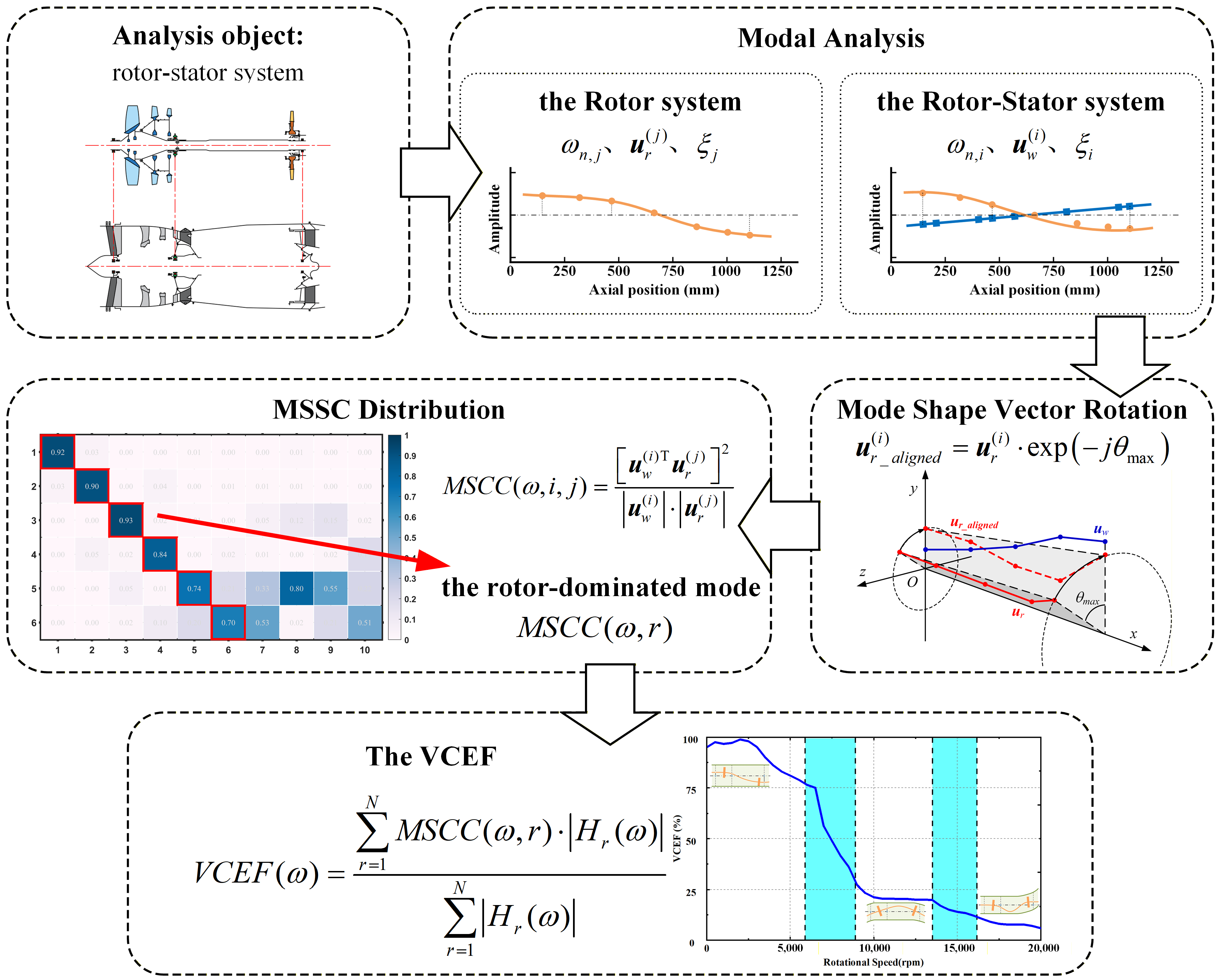
The previous section introduced the theoretical part of the VCEF method. Next, this section will provide a detailed introduction to the calculation procedure of the quantitative evaluation method, as shown in Figure 4. The VCEF calculation follows these steps:

(1)

Analysis object: Establish the rotor–stator system of the aeroengine as the analysis object. Input the system parameters, including geometry, material, damping, and so on. The finite element model of the rotor system and the rotor–stator system would be established.

(2)

Modal analysis: Conduct modal analysis on the rotor system and the rotor–stator system and extract the natural frequency, mode shape vector, and damping ratio.

(3)

Mode shape vector rotation: Rotate the mode shape vectors based on Equation (23) to realign phase angles, eliminating correlation errors.

(4)

MSCC distribution: Calculate the MSCC for each mode based on Equation (22) and obtain the MSCC distribution. Furthermore, identify the rotor-dominated modes based on Equation (24).

(5)

the VCEF: Iteratively compute the MSCC distribution versus various rotational speeds and calculate the VCEF based on Equation (25).

3. Application to a Simplified Rotor–Stator System

To validate the effectiveness of the proposed quantitative evaluation method, a simplified rotor–stator system with low DOFs is constructed. This example illustrates the practical application of the VCEF and its capability in assessing the degree of vibration coupling in the rotor–stator system.

3.1. Model Setup

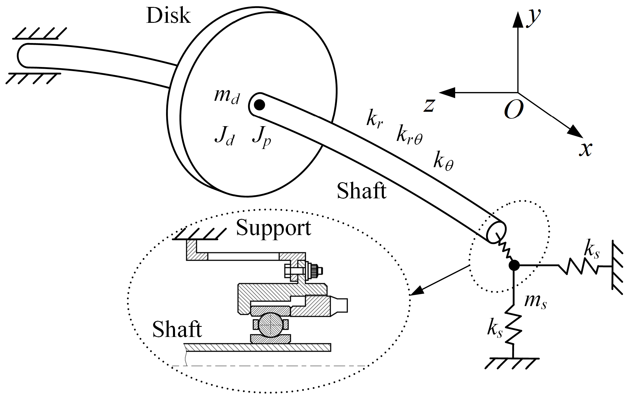
A single-disk, non-midspan rotor model is established as an example model, as shown in Figure 5. The system consists of a rotor mounted on a flexible support, forming a rotor–stator system that enables comparative analysis between the rotor system and the rotor–stator system.

The rotor–stator system has six DOFs: four DOFs for the rotor component and two DOFs for the stator component. The generalized coordinates are defined as follows:

$${\mathit{q}}_{\mathit{r}}={\left\{\begin{array}{cccc}{y}_d& z_d& {\theta }_y& {\theta }_z\end{array}\right\}}^T$$

(26)

$${\mathit{q}}_{\mathit{w}}={\left\{\begin{array}{cccccc}{y}_d& z_d& {\theta }_y& {\theta }_z& y_s& z_s\end{array}\right\}}^T$$

(27)

where $y_d$ and $z_d$ represent the translational displacement of the rotor disk, ${\theta }_y$ and ${\theta }_z$ denote its rotational displacements, and $y_s$ and $z_s$ correspond to the translational movements of the support (stator).

The parameters of the example model are as follows: the rotor disk is characterized by its mass $m_d$ and rotational inertias $J_d$, $J_p$. The shaft provides translational stiffnesses $k_r$, rotational stiffness $k_{\theta }$, and coupling stiffness $k_{r\theta }$. The stator mass is denoted as $m_s$, and its constraint stiffness is $k_s$. In addition, structural damping $c$ is introduced as a material property to represent energy dissipation.

Based on Equations (6) and (7), the motion equations and the parameter matrices of the example model can be obtained. To ensure that the research has broader significance, the system parameters are dimensionless, adopting the following reference quantities: $m_d=10$, $J_p=0.8$. $J_d=10$, $m_s=1$, $k_{rr}=k_r+k_s=1000$, $k_{r\theta }=2000$, $k_{\theta }=1000$, and $c=0.03$. In addition, the rotor–stator stiffness ratio $\alpha =k_r/k_{rr}=0.2$.

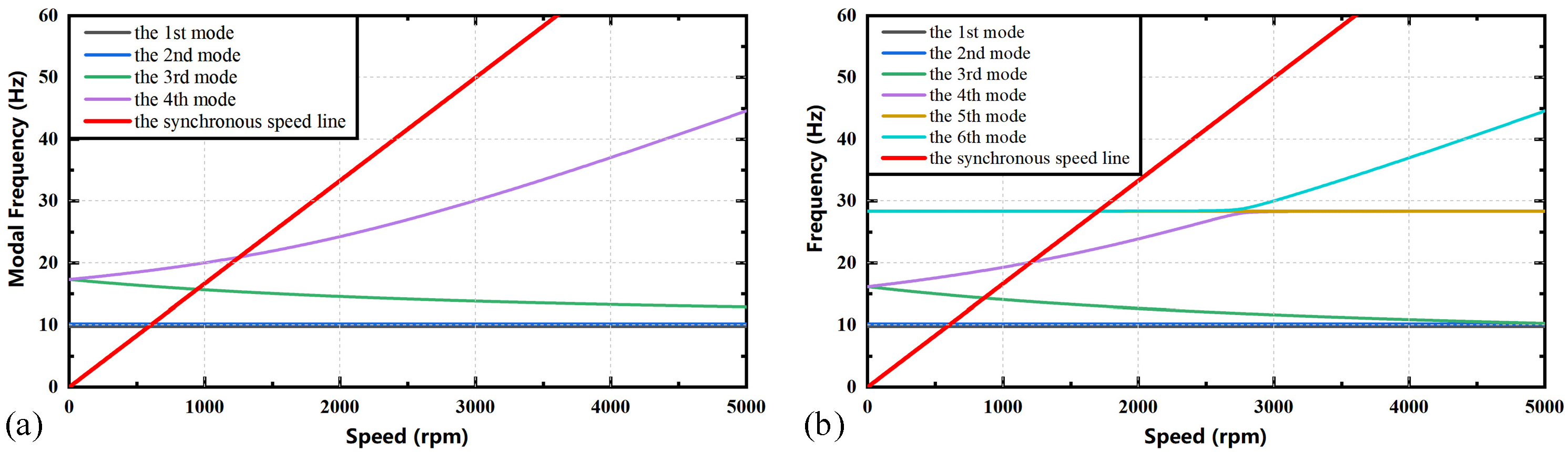
The dynamic characteristics of the example model have been calculated based on the given parameters and the Campbell diagrams are shown in Figure 6. It can be observed that there are two types of rotor-dominated modes in the example model: the lateral motion of the disk (corresponding to the 1st and 2nd modes) and the deflection motion of the disk (corresponding to the 3rd and 4th modes). Among them, the deflection motion mode will be affected by the gyroscopic effect, and the modal frequencies of the forward and backward modes will be affected by the rotational speed. Additionally, different from the rotor system, the additional stator-dominated mode emerges at 28.37 Hz in the rotor–stator system, which corresponds to the 5th and 6th modes in Figure 6b.

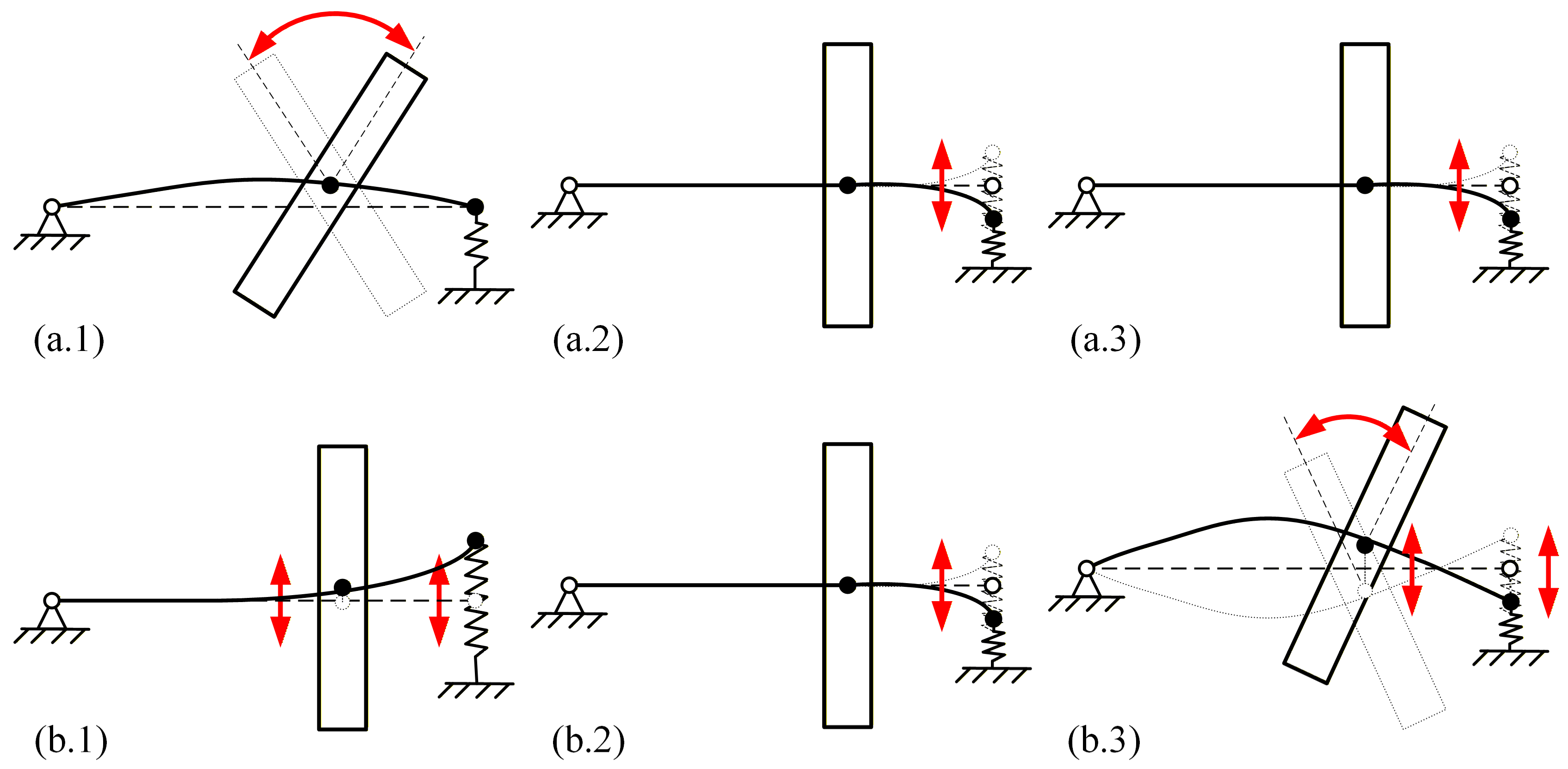
It needs to be noted that there is a mode shape transformation of the 4th, 5th, and 6th modes near 2700 rpm. As shown in Figure 7(a.2,b.2), the mode shape of the 5th mode remains virtually unchanged—it consistently represents a local deformation of the stator. In contrast, the 4th and 6th mode shapes undergo a notable transformation. At low speeds, the 4th mode is characterized by deflection motion of the disk, while the 6th mode involves local stator deformation (orthogonal to the 5th mode’s deformation direction). As the rotational speed increases, mode shape transformation occurs: the 4th mode shape transitions to being dominated by stator deformation with minor rotor lateral motion, and the 6th mode transitions to being dominated by deflection motion of the disk accompanied by slight lateral motion of both the rotor and stator.

A correspondence can be established between the low-speed and high-speed mode shapes in Figure 7, where (a.1) corresponds to (b.3), (a.2) to (b.2), and (a.3) to (b.1). This phenomenon occurs because the gyroscopic effect significantly alters the mode shapes associated with rotor-dominated modes as their frequencies approach those of stator-dominated modes. This frequency convergence leads to modal coupling between the rotor and stator, namely rotor–stator vibration coupling, manifested as a transformation of the mode shapes among several modes.

3.2. Evaluation Results of the VCEF

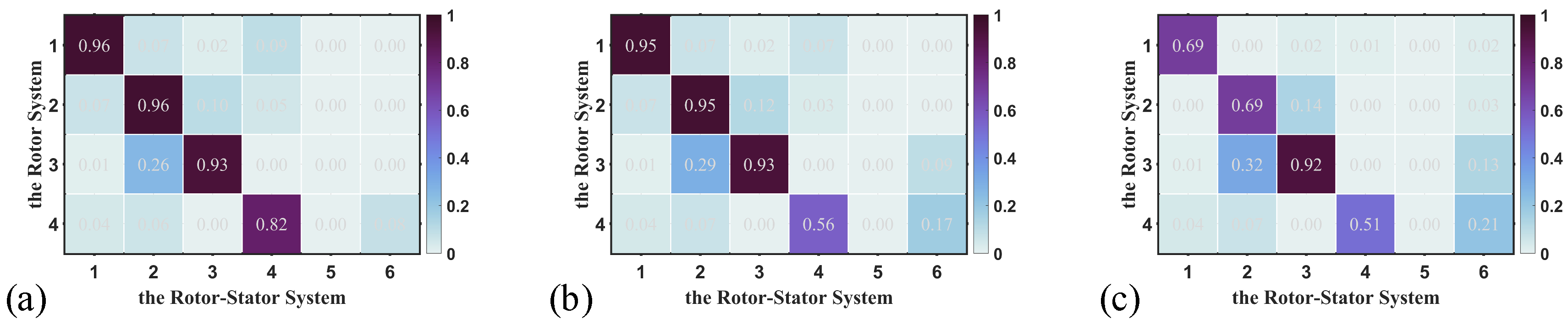
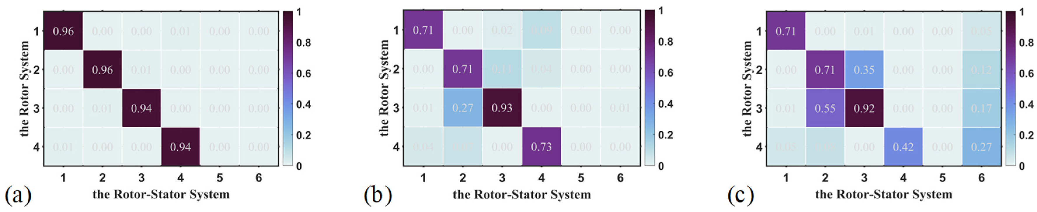
To quantify the similarity between the mode shapes of the rotor system and the rotor–stator system, the MSCC has been calculated according to Equation (22) using the mode shape vectors obtained based on the modal analysis results. The MSCC distribution, as shown in Figure 8, reveals how the mode shapes change with rotational speed and allows for a quantitative evaluation of the similarity of mode shapes at different rotational speeds.

It can be observed from Figure 8a that there is an obvious one-to-one correspondence between the first four mode shapes of the rotor system and those of the rotor–stator system at 0 rpm. The MSCC values on the diagonal are all above 0.9, while the values at other positions are close to 0. Therefore, it can be considered that the influence of the stator on the mode shapes of the rotor component is little and there is weak vibration coupling between the rotor and stator.

However, as the rotational speed increases, the similarity gradually diminishes, as shown in Figure 8b,c. The MSCC values on the diagonal decrease significantly. For example, the MSCC between the 4th mode of the rotor–stator system and the rotor system drops from 0.73 at 2500 rpm to 0.42 at 5000 rpm.

Conversely, some off-diagonal MSCC values increase, indicating increased rotor–stator vibration coupling. For example, the MSCC between the 2nd mode of the rotor–stator system and the 3rd mode of the rotor system increases from 0.27 for MSCC (2500,2,3) to 0.55 for MSCC (5000,2,3).

Also, there is some similarity between the mode shape of the rotor system and the stator-dominated mode shape, such as the MSCC between the 6th mode of the rotor–stator system and the 4th mode of the rotor system; the MSCC (5000,6,4) becomes 0.27, which can serve as evidence of the vibration coupling of the rotor and stator.

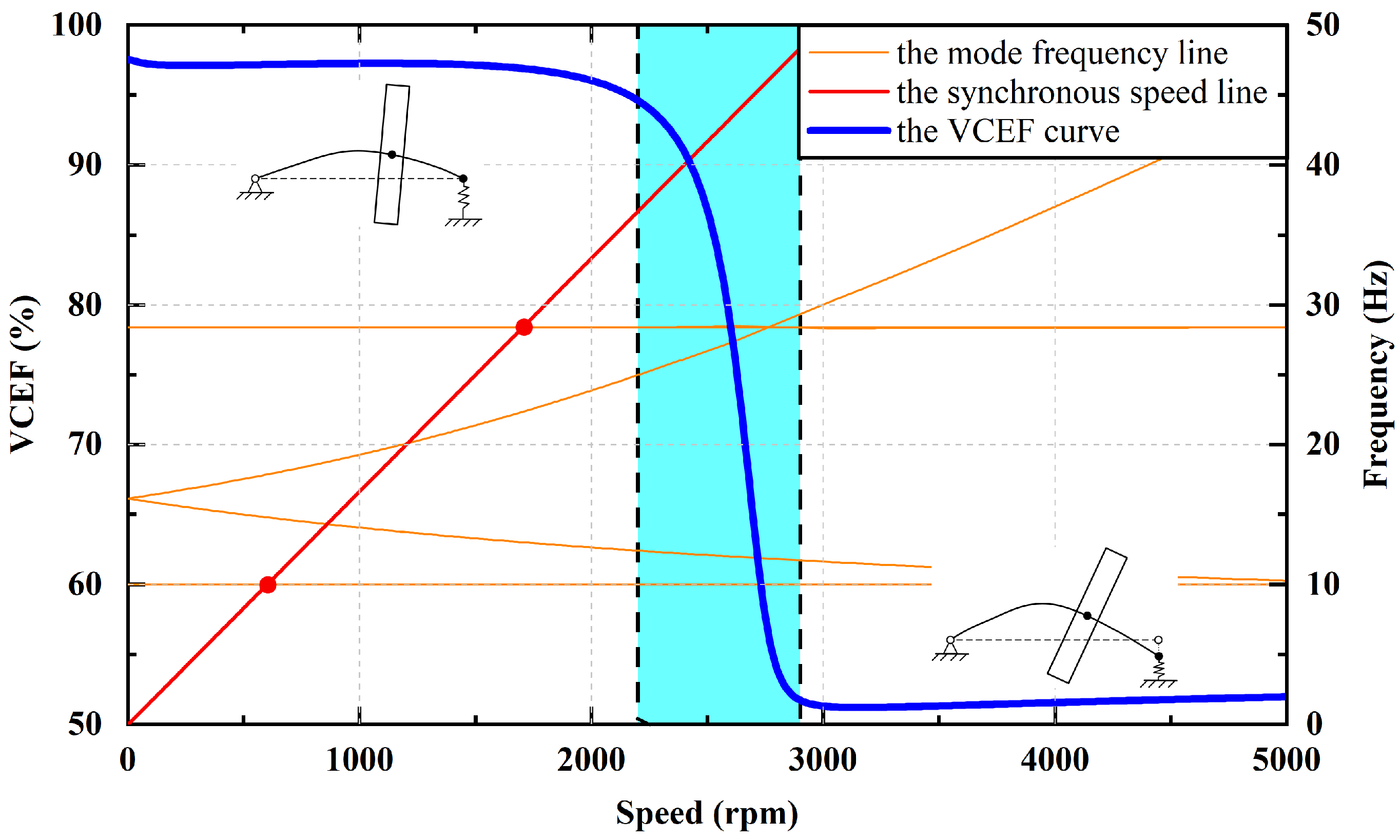
Based on the evaluation method, the VCEF values versus rotational speeds were computed. Because the example model is a single rotor–stator system and the forward mode shapes dominate the dynamic response under imbalance loading, the second and fourth modes have been selected for quantitative evaluation. However, if the analysis object is a counter-rotating dual rotor–stator system, both forward and backward mode shapes need to be calculated. The MSCC values for these modes are extracted and substituted into Equation (25) for calculation. The VCEF values versus rotational speed are plotted with the blue line in Figure 9. For the convenience of comparing the changes in the VCEF, a Campbell diagram of the rotor–stator system has also been drawn in Figure 9, with orange lines for the mode frequency lines and a red line for the synchronous speed line. The following observations can be made:

At low speeds (<2300 rpm): The VCEF remains above 90% and the rotor deformation is dominated in the deformation of the rotor–stator system, indicating a high degree of similarity between the rotor system and the rotor–stator system, suggesting weak vibration coupling.

At intermediate speeds (2300~2800 rpm): The VCEF drops sharply to about 50%, coinciding with the transition of mode shapes, which is reflected in the Campbell diagram. It can be seen from Figure 9 that at 2500~3000 rpm, the transition of the 4th, 5th, and 6th mode shapes emerges and the VCEF drops at the same time, signaling a significant increase in rotor–stator vibration coupling.

The MSCC distributions at multiple rotational speeds during the drop of the VCEF are shown in Figure 10 to study the mechanism of the VCEF change process. It can be seen that in the range of 2200–2800 rpm, the change in the MSCC distribution is mainly concentrated in the MSCC (w,4,4) and MSCC (w,6,4), with little change in other positions.

Due to the mode shape transformation, the similarity between the 4th mode of the rotor system and the 4th mode of the rotor–stator system MSCC (w,4,4) decreases significantly, accompanied by a significant increase in similarity with the 6th mode MSCC (w,6,4). It can be considered that the mode shapes of the rotor component are changed due to the stator, that is, the rotor–stator vibration coupling, accompanied by a change in VCEF values.

At high speeds (>2800 rpm): the VCEF remains consistently at a low level. There is not only the lateral and deflection deformation of the rotor, but also the deformation of the stator in the rotor–stator system, suggesting significant vibration coupling. However, the values of VCEF slightly increased as the speed increased. It is speculated that in the high-speed range, the weight of the 2nd mode increased compared to that of the 4th mode, as the value of MSCC (w,2,2) is relatively high.

It can be seen from Figure 9 that the VCEF value stabilized around 0.97 below 2300 rpm. It then dropped rapidly to 0.53 within 2300–2800 rpm, indicating the effect of vibration coupling. Through the stepped decrease in VCEF values, it can be found that the dynamic response of the rotor–stator system is significantly different from that of the rotor system due to rotor–stator vibration coupling. The similarity between the dynamic characteristics of the two systems became low in the high-speed range, and if the dynamic analysis is based on the dynamic response of the rotor system, it may deviate from engineering practice.

3.3. Parameter Sensitivity Analysis

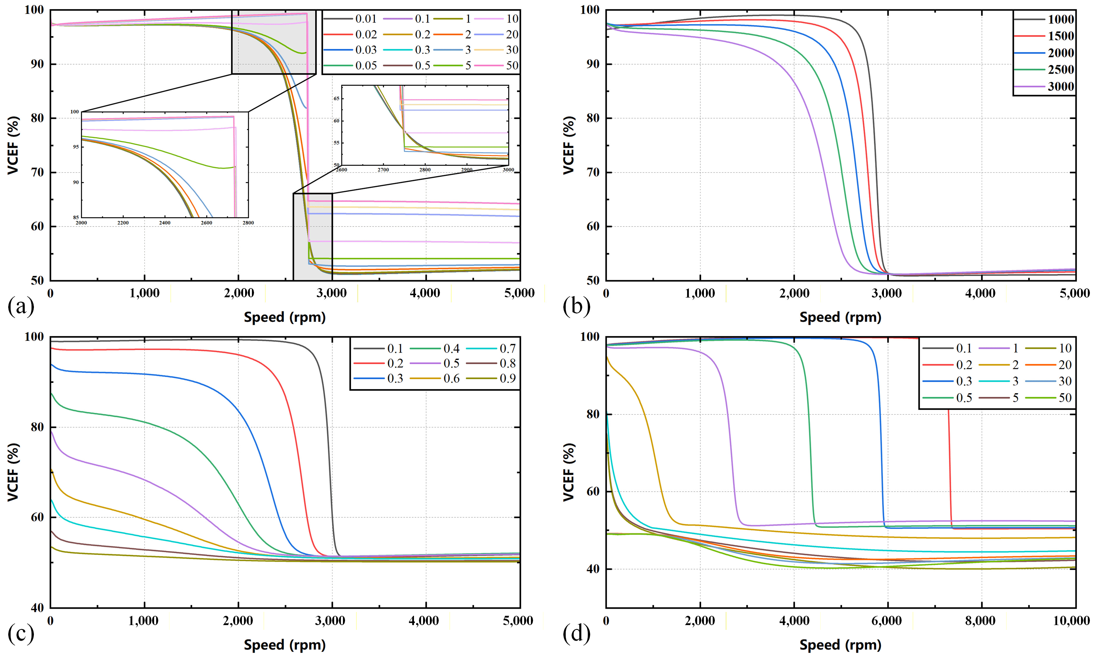
To further explore the impact of structural parameters on vibration coupling, sensitivity analyses were conducted by varying key system properties and repeating the quantitative evaluation method, including the structural damping $c$, the coupling stiffness $k_{r\theta }$, the rotor–stator stiffness ratio $\alpha =k_r/k_{rr}$, and the stator mass $m_s$. It should be noted that this section is just for sensitivity analysis, and some values may have significant differences from those in an actual situation. The influence of different parameters on the VCEF is shown in Figure 11, and the following observations can be made:

(1) The Structural Damping $c$. It can be seen from Figure 11a that the VCEF values versus rotational speed are not affected by the structural damping value. However, the large structural damping (c > 2 in this example model) will cause the downward trend of VCEF to transition from “smooth” to “step”. Therefore, appropriately reducing the structural damping helps to make the change process of VCEF smoother. In addition, the significant structural damping (c > 10 in this example model) may increase the VCEF value in the high-speed range, but it is not feasible in engineering practice.

(2) The Coupling Stiffness $k_{r\theta }$. It can be seen from Figure 11b that the VCEF values versus rotational speed are not affected by the coupling stiffness of lateral and deflection motion. Higher coupling stiffness leads to a gradual rather than abrupt decline in VCEF, distributing the coupling effect over a broader speed range. When the coupling stiffness is low, the VCEF will slightly increase with the speed in the low-speed range and suddenly decrease when it reaches the speed range of the rotor–stator vibration coupling. As the coupling stiffness gradually increases, the VCEF slightly decreases and the stepwise decline emerges at the lower rotational speed. Overall, lower coupling stiffness is beneficial for increasing the speed range in which rotor–stator vibration coupling occurs.

(3) The Rotor–Stator Stiffness Ratio $\alpha$. By making the stiffness $k_{rr}$ of the lateral motion constant, adjusting the rotor–stator stiffness ratio $\alpha$, different combinations of rotor and stator stiffness can be obtained, thereby facilitating the study of the influence of the ratio of stator stiffness to rotor stiffness on vibration coupling, as shown in Figure 11c. It can be observed that the influence of the rotor–stator stiffness ratio $\alpha$ is concentrated in the low-speed range. When the ratio $\alpha$ is smaller than 0.3, the values of the VCEF are much higher in the low-speed range. When the rotor–stator stiffness ratio $\alpha$ is high, the VCEF values will decrease steadily with the rotational speed. And as the proportion of stator stiffness gradually increases, the stepwise decline in VCEF values will emerge at the lower rotational speed, indicating that the influence range of the stator component gradually expands until the full speed range is reached. Therefore, the rotor stiffness must be large enough, compared to the stator stiffness, to achieve the influence of stator components on the dynamic characteristics of the rotor–stator system over a sufficiently large speed range.

(4) The Stator Mass $m_s$. It can be seen from Figure 11d that under the premise of unchanged rotor mass ($m_d$ = 10 in this model), changes in the stator mass will have a significant influence on the phenomenon of rotor–stator vibration coupling. That is, the ratio of stator mass to rotor mass has a significant impact on the coupling phenomenon. When the stator mass is low ($m_s$ < 1), the VCEF can maintain a high value in the low-speed range and then drop rapidly. Moreover, the smaller the stator mass, the higher the rotational speed where the VCEF values drop stepwise. As the stator mass continues to increase ($m_s$ > 2), the VCEF will always stabilize around 0.5, indicating that the influence of the stator mass on the rotor–stator system expands to the entire speed range. The stator mass continues to increase to be greater than the rotor mass ($m_s$ > 10), and the VCEF values will be smaller than 0.5 and slightly decrease throughout the entire speed range, indicating that the influence of stator mass on the vibration coupling of the rotor–stator system no longer changes with speed. Therefore, the stator mass should be minimized as much as possible, so that the operating speed range can be positioned with the high VCEF, where vibration coupling effects are minimal.

This example model demonstrates the applicability of the proposed quantitative evaluation method in quantifying rotor–stator vibration coupling in this section. It can be found that the VCEF effectively captures the transition point where vibration coupling becomes significant. In addition, structural parameters, such as stator stiffness and stator mass, significantly influence vibration coupling. And there are few influences of the structure damping and the coupling stiffness on the VCEF values. These findings not only validate the effectiveness of the VCEF but also provide valuable insights for the design and optimization of high-speed rotating machinery, highlighting the importance of considering these parameters in engineering practice.

4. Application to a Complex Rotor–Stator System

To validate the effectiveness of the proposed quantitative evaluation method, a rotor–stator system was derived from a certain type of aeroengine through numerical analysis. This system illustrates the practical application of the VCEF and its capability in assessing the degree of vibration coupling in a rotor–stator system through the simulation and experimental studies. And the evaluation results were validated through the experiments in Section 5.

4.1. Model Setup

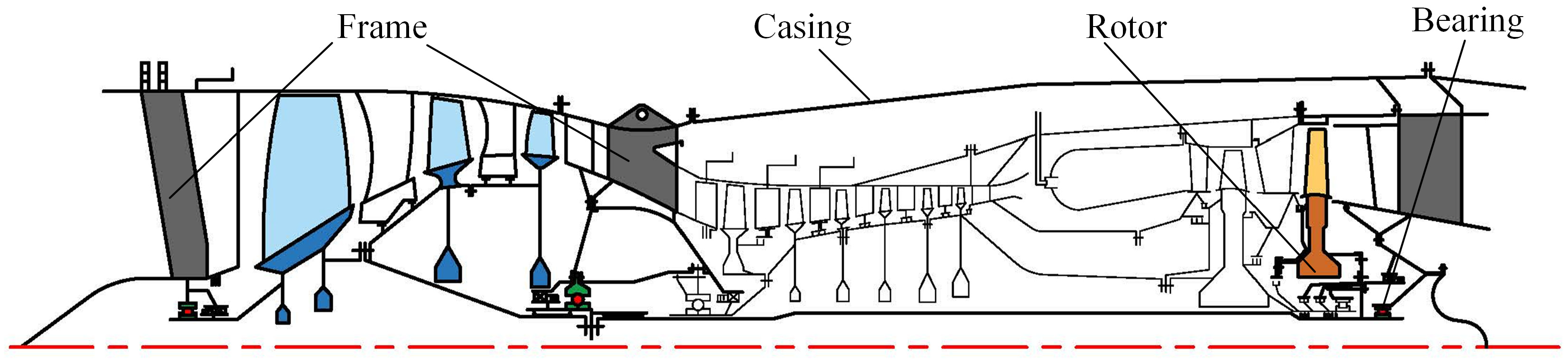
A comprehensive dynamic analysis was performed on a physics-based abstraction of the LP rotor–stator system extracted from a certain type of high-thrust-to-weight-ratio turbofan engine, as shown in Figure 12.

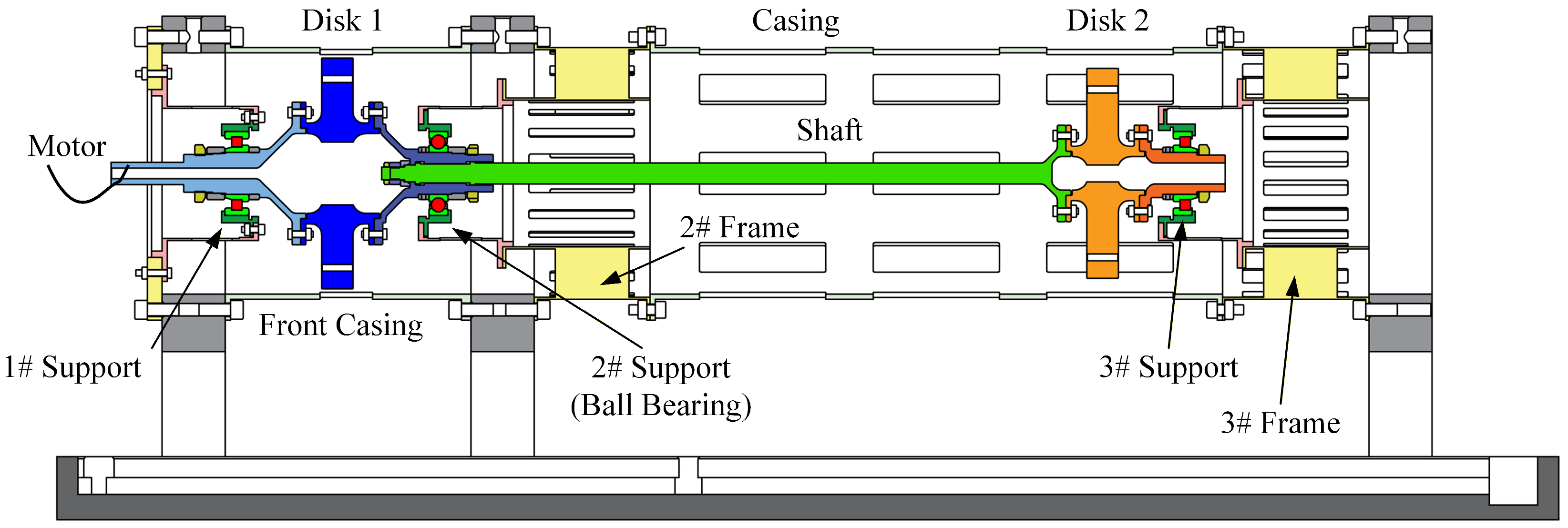
The schematic of the rotor–stator system is shown in Figure 13. Some details of the experimental research were considered during the rotor–stator system designed in order to facilitate subsequent experimental research and compare the results of the simulation and experimental results. The rotor–stator system in this paper was designed with reference to the low-pressure rotor [2], which simulates an operating rotational speed of 7000–8000 rpm, and its corresponding stator of a Low-Bypass Turbofan Engine.

There are three supporting bearings, where there is Disk 1 between the 1# and 2# Supports, and Disk 2 and the slender shaft are between the 2# and 3# Supports, which feature a large span and low stiffness. Among them, a ball bearing was used at the 2# Support, which offers axial positioning for the rotor, while the rolling bearings are used at other supports. In addition, the shaft segment at the 1# Support is connected to the motor in the tester to obtain torque input.

On the stator, each bearing and its corresponding bearing seat were installed. The stator at the 2# and 3# Support, namely the 2# Frame and the 3# Frame, was designed with reference to the stator in the Low-Bypass Turbofan Engine, which is the dual-layered, thin-walled frame structure, interconnected via longitudinal plates. The casing is situated between the 2# and the 3# Frames, which is installed via the flange edges and bolts, and the front casing is installed between the 1# and the 2# Supports. In order to regulate the stiffness of the stator, the thickness of the casings and frames were adjusted and several slots were uniformly designed in the circumferential direction in the casing and frame. In addition, the split casing design scheme was adopted for the convenience of installation.

4.2. Simulation Result

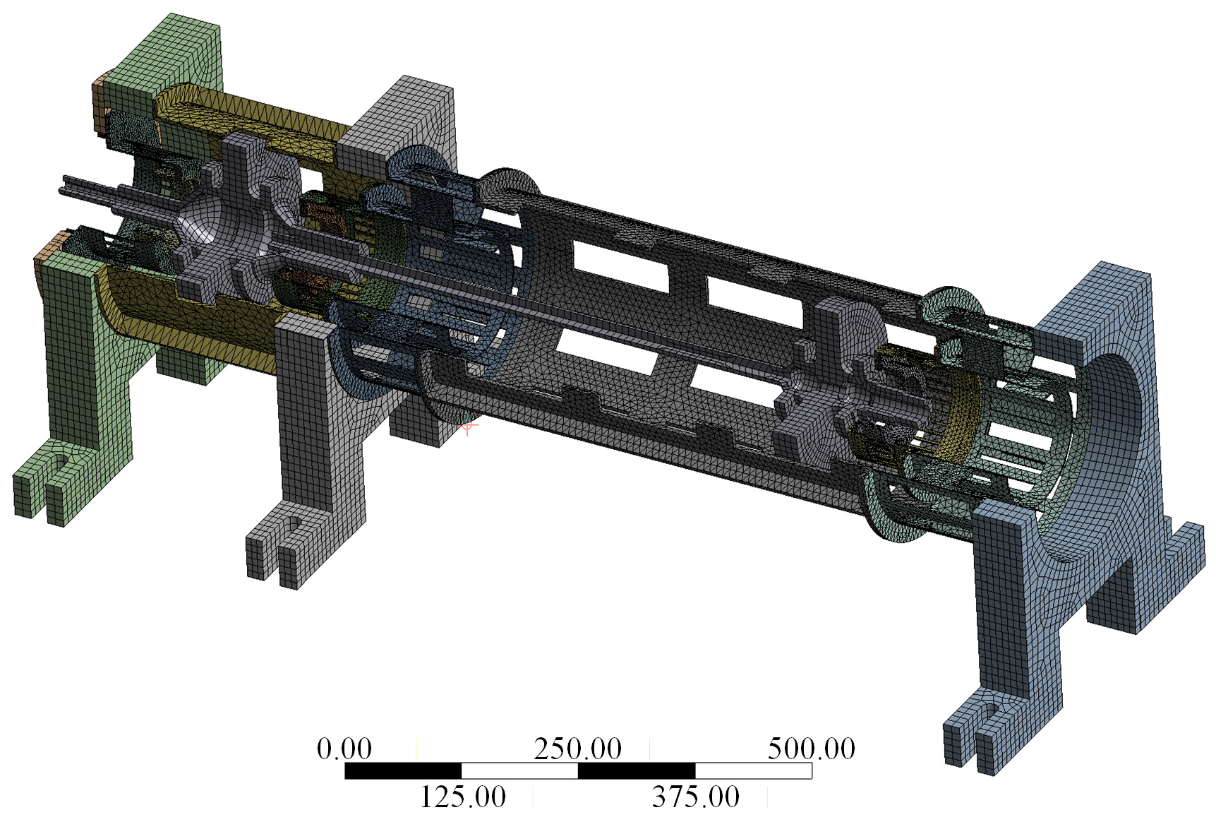
The rotor–stator system and the rotor system were discretized by SOLID 186 element to obtain the finite element mode, as shown in Figure 14. The material of the finite element models is steel. The modal analysis was performed on the finite element models. Campbell diagrams of the rotor–stator system and the rotor system are shown in Figure 15.

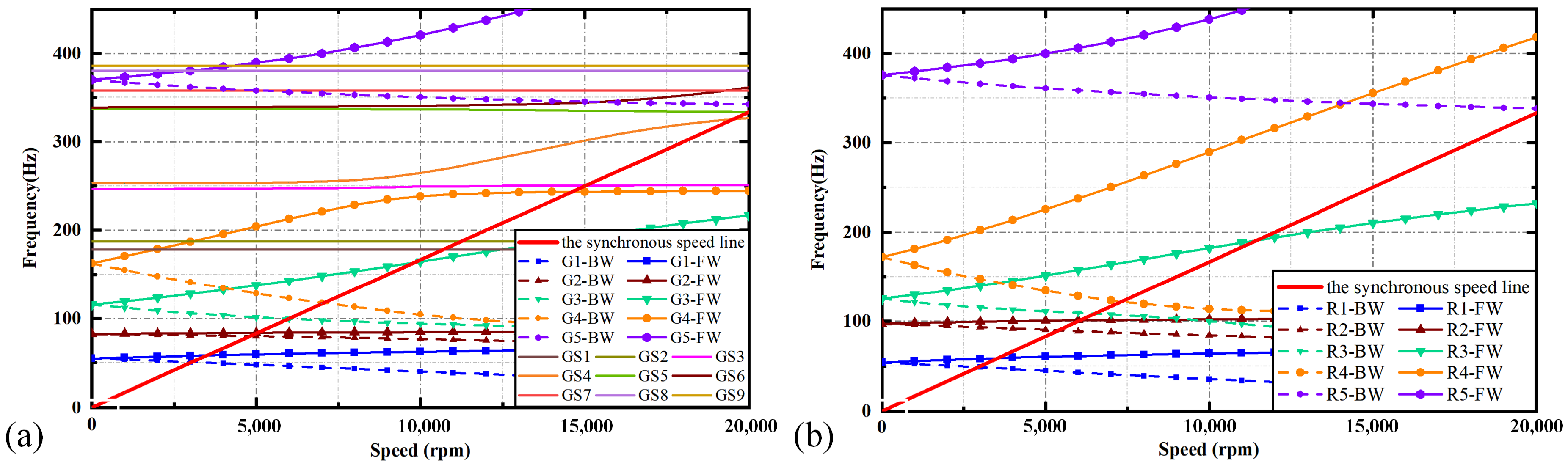
It can be seen from Figure 15a that there are five pairs of rotor-dominated modes (G1, G2… G5) and nine pairs of stator-dominated modes (GS1, GS2… GS9) within 450 Hz in the rotor–stator system. In Figure 15a, the forward (FW) mode frequency lines are represented by the solid lines with symbols, the backward (BW) mode frequency lines are represented by the dashed lines with symbols, and the mode frequency lines of the stator-dominated mode are represented by the solid lines without symbols. Similarly, it can be seen from Figure 15b that there are five pairs of modes (R1, R2… R5) in the rotor system. The constant speed lines of the Campbell diagram are presented by the red bold solid line.

It can be seen from Figure 15a that there are three intersection points between the constant speed line and the mode frequency lines G1-FW, G2-FW, and G3-FW, respectively, at 3510, 5097, and 9913 rpm. These intersections indicate that the system has three critical rotational speeds within the operating speed range. When the rotational speed approaches these three critical rotational speeds and there is excitation at the corresponding positions, significant dangerous dynamic responses will occur in the rotor stator structure. From the comparison between Figure 15a,b, it can be seen that the mode frequency distribution of the two systems is relatively close, and the differences are mainly concentrated in the mode frequency lines of the stator-dominated mode in the rotor–stator system. Subsequently, the influence of rotor–stator vibration coupling on dynamic response will be discussed based on the similarity.

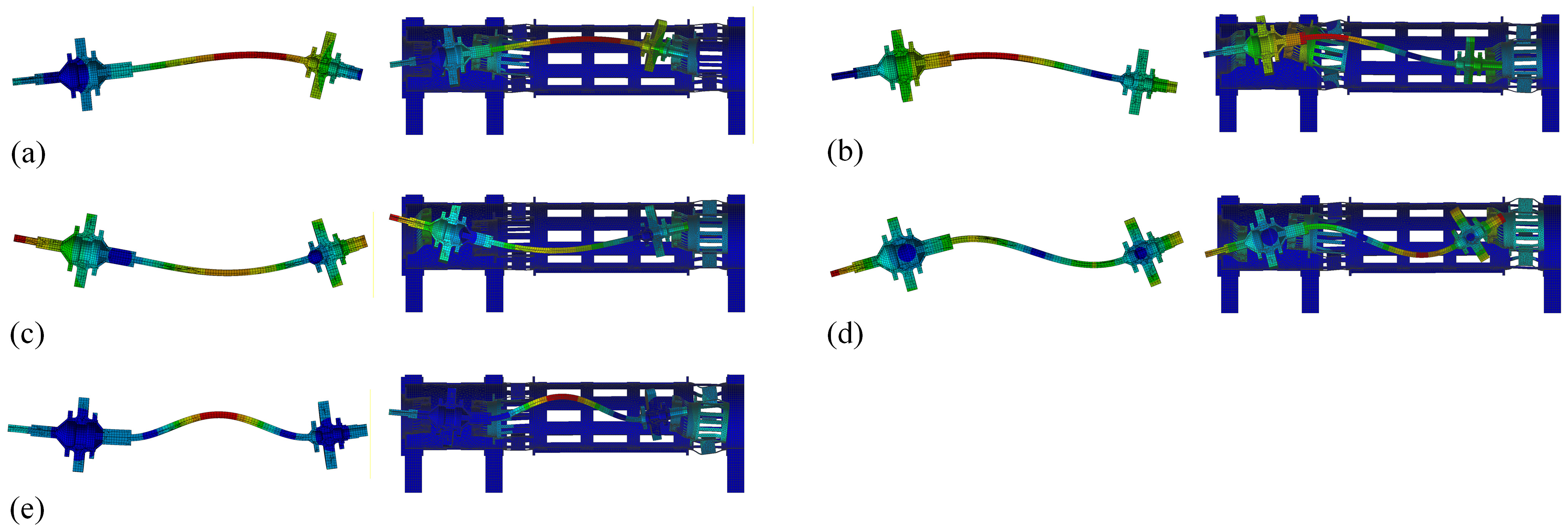
It can be known that the rotor-dominated mode of the rotor–stator system is more readily excited during rotation, leading to a greater impact on the dynamic characteristics of the research object. Moreover, there exists a corresponding relationship between them with the modes of the rotor. Figure 16 compares the rotor-dominated modes of the rotor system and the rotor–stator systems at 0 rpm, with ‘R’ indicating the rotor system and ‘G’ representing the rotor–stator system. It can be seen that the various rotor-dominated modes of the rotor–stator system have a high degree of similarity with the rotor system, and it is easy to determine the correspondence between the rotor-dominated modes in the two systems.

However, there are significant deformations that cannot be ignored at the stator in the mode shapes of various rotor-dominated modes of the rotor–stator system, although they are much smaller than that of the rotor. For example, in the G2 mode shape shown in Figure 16b, there is an obvious deformation at the bearings and the frames. Moreover, the rotor deformation was influenced by the stator, which is also a manifestation of the rotor–stator vibration coupling. For example, there is a difference in rotor deformation between the R5 mode and the G5 mode, which can be seen from the deflection angle of Disk 1 as shown in Figure 16e, and which is due to the deformation of the 3# Frame in the G5 mode.

4.3. MSCC Distribution

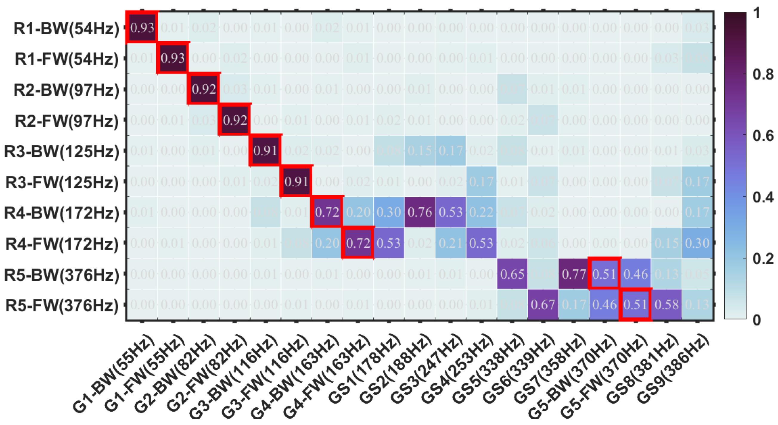
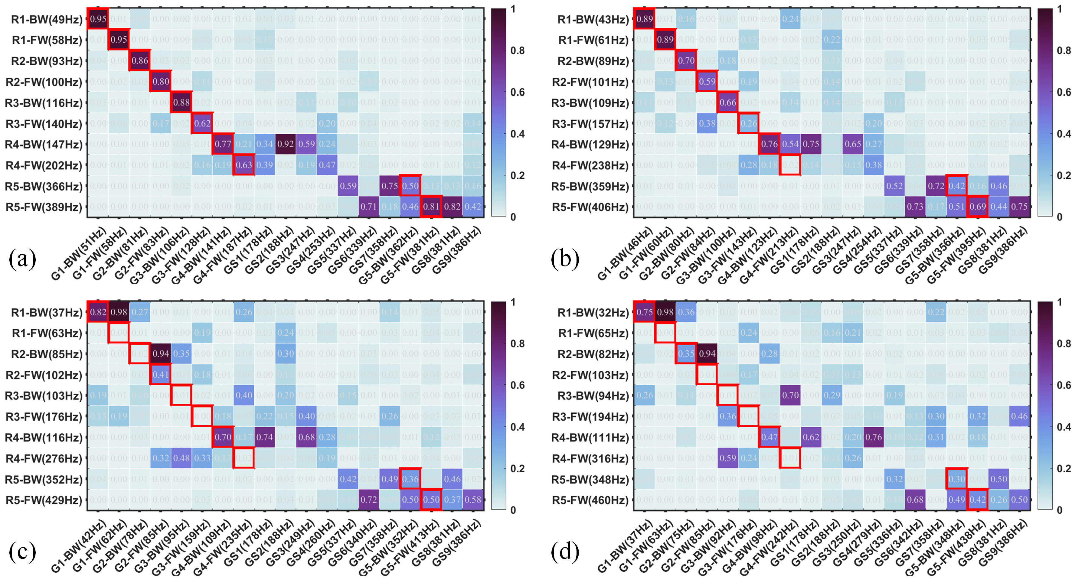
Based on the modal analysis results, the mode shape vectors were obtained and the MSCC could be calculated according to Equation (22). The MSCC is presented as a distribution diagram in Figure 17 and Figure 18, where the horizontal and vertical axes represent the modes of the rotor–stator system and rotor system, respectively, labeled with the abbreviations and corresponding modal frequencies at different rotational speeds.

Similar to most MSCC distribution diagrams, there is a MSCC value that is relatively high in each row or column and generally appears at the diagonal position. Due to the difference in the number of modes between the two systems in this paper, the diagonal position is inconsistent. However, there is a correspondence between the rotor-dominated modes of the two systems, as shown in Figure 17, and the corresponding positions are circled in red boxes in the MSCC distribution diagram for easy understanding.

It can be seen from Figure 17 that the MSCCs of low-order rotor-dominated modes are generally higher and close to 1, while the MSCCs of the other modes are lower. There is a clear correspondence between the rotor-dominated modes of the rotor system and the rotor–stator system at 0 rpm, and the main reason is that the rotor deformation in the mode shape is less affected by the stator and the rotor–stator vibration coupling is weak in low-order rotor-dominated modes.

However, as the order increases, there is a decrease in MSCC of the rotor-dominated modes. It can be seen from Figure 17 that the MSCC values of FW rotor-dominated modes are 0.93, 0.92, and 0.91 for the first three orders, but 0.72 and 0.51 for the fourth and fifth orders, respectively. Also, the corresponding relationship of the rotor-dominated modes gradually becomes weak. Taking the R5-FW mode as an example, it can be seen from Figure 17 that there are four MSCC values greater than 0.3 between R5-FW and the modes of rotor–stator system, and the MSCC value between R5-FW and GS6 is 0.67, which is even greater than the MSCC value between R5-FW and G5-FW of 0.51. Therefore, it can be found that one mode shape of the rotor system is similar to the several mode shapes of the rotor–stator system.

The possible reason for this phenomenon may be that there is a significant impact on the rotor deformation from the stator. On the one hand, the rotor-dominated modes undergo changes due to the influence of the stator; on the other hand, the rotor deformation is also contained in the stator-dominated modes. It can be concluded that as the mode order increases, the rotor–stator vibration coupling intensifies. That is, the higher the mode frequency, the more rotor–stator vibration coupling components in the mode shape.

The comparison of the MSCC distribution at different rotational speeds is shown in Figure 18. It can be seen that the MSCC values corresponding to each rotor-dominated mode significantly decrease as the rotational speed increases. Taking the R2-FW and G2-FW modes as an example, the MSCC values are 0.92, 0.80, 0.59, 0.41, and 0.01 as the speed increases. So, it can be concluded that, similar to the modal frequency, as the rotational speed increases, there are more rotor–stator vibration coupling components in the mode shape.

It also can be seen from Figure 18 that, as the rotational speed increases, the MSCC distribution between the rotor-dominated modes gradually loses a recognizable corresponding relationship. The MSCC distribution at 3000 rpm shown in Figure 18a is similar to that at 0 rpm shown in Figure 17. However, in the distribution at 6000 rpm shown in Figure 18b, there is a significant increase in MSCC values between the rotor-dominated modes and some other modes, and the corresponding relationship is partially weakened.

However, when the rotational speed is at a high level, the corresponding relationship between the MSCC values of the rotor-dominated modes will become extremely weak, as shown in Figure 18c,d. The similarity in modal characteristics between the two systems can no longer be determined through MSCC distribution. It can be considered that there is significant rotor–stator vibration coupling under this phenomenon.

The possible reason for this phenomenon may be that the gyroscopic effect generated during the rotor rotation not only affects the modal frequency and mode shape of the rotor, but also transmits from the rotor to the stator, which has a significant impact on the dynamic characteristics of the entire system.

4.4. Evaluation Result of the VCEF

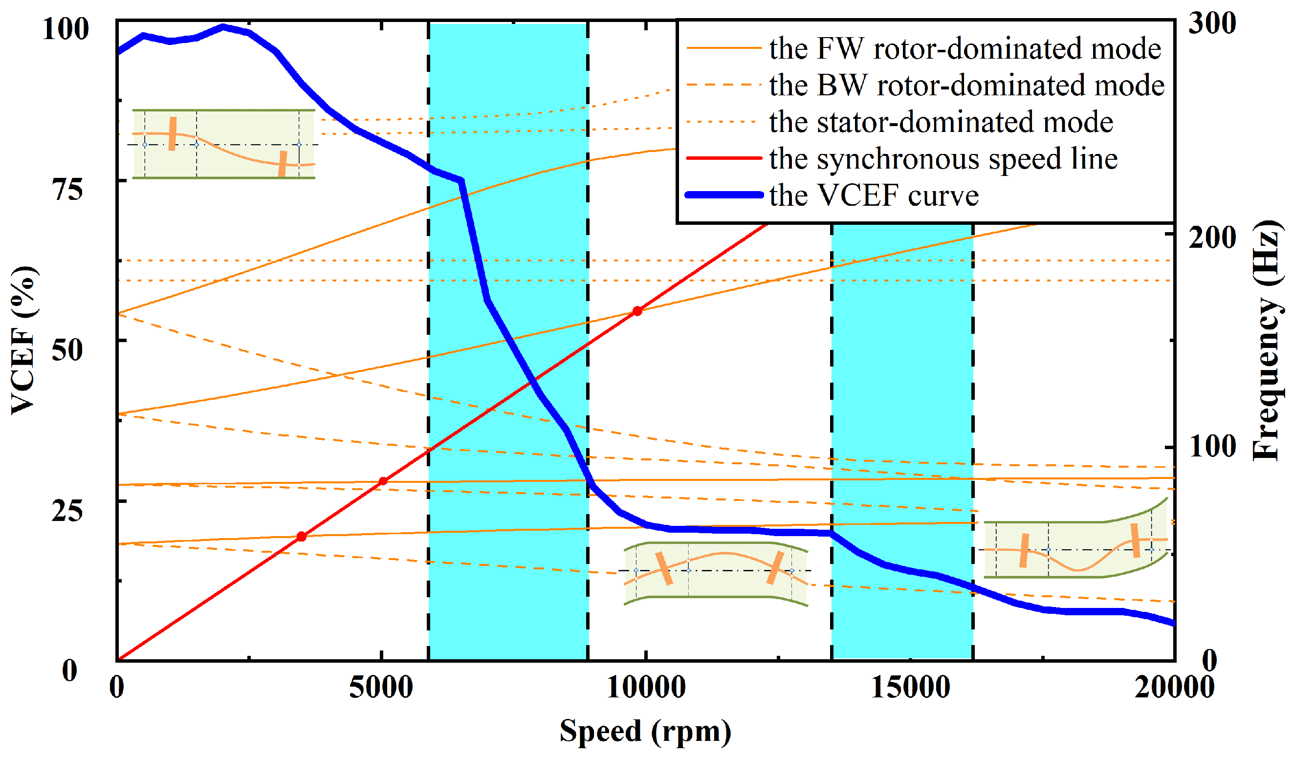
The MSCC values of rotor-dominated modes at different rotational speeds were used to calculate the VCEF according to Equation (25), and the analysis process is shown in Figure 4. The variation in the VCEF with rotational speed is shown in Figure 19. For the convenience of comparing the changes in the VCEF, a Campbell diagram of the rotor–stator system has also been drawn in Figure 19, with a red line for the synchronous speed line and orange lines for the mode frequency lines. Among the orange lines, the solid lines represent the FW rotor-dominated mode, the dashed lines represent the BW rotor-dominated mode, and the dotted lines represent the stator-dominated mode.

It can be seen from Figure 19 that the VCEF values generally show a monotonically decreasing trend as the rotational speed increases. Within 3000 rpm, the rotor operates at the subcritical state and there are few deformations of each stator-dominated mode shape. Therefore, the rotor–stator vibration coupling is weak and the VCEF value is near to 1. When the speed exceeds 3510 rpm, the 1st critical speed, the rotor operates in the supercritical state, and there will be rotor–stator vibration coupling in the dynamic behavior. The VCEF values stabilizes above 0.75 in the range of 3000~6000 rpm and slightly decreases with the rotational speed, indicating slight rotor–stator vibration coupling within this rotational speed range. When the speed reaches 6000 rpm, the VCEF value drops rapidly to 0.25 within 6000–9000 rpm, the light blue range in Figure 19. Therefore, it can be considered that when the speed is above 6000 rpm, the rotor–stator vibration coupling of this rotor–stator system cannot be ignored, which will also be verified in the experimental results. Moreover, it can be observed that while rotor deformation occurs, the stator also exhibits non-negligible deformations during operation.

Furthermore, as shown in Figure 19, there is another stepped decrease in the VCEF curve within the higher rotational speed range of 13,500–16,000 rpm, although the decrease amplitude is less. Additionally, the proportion of deformation attributed to the stator demonstrated a marked increase during operation. Different from the example model discussed earlier, for complex systems with multiple DOFs, there may be multiple rotational speed ranges where the VCEF values drop rapidly, which may lead to the segmented enhancement of the rotor–stator vibration coupling.

Above all, the rotor–stator vibration coupling is relatively weak in the low rotational speed range with the high values of VCEF, and the rotating machinery is suitable to be analyzed according to the traditional rotor dynamics; if the operating rotational speed is such that the VCEF values drop rapidly or stabilize around low value, the rotor–stator vibration coupling is significant and needs to be analyzed using the rotor–stator system in design and verification. It is noted that the absolute value of the VCEF can vary across different rotor–stator systems. However, a sharp decrease in the VCEF within the speed range is identified as a key indicator, signifying the onset region of rotor–stator vibration coupling.

5. Experimental Results

The rotor–stator system was built to conduct dynamic experiments and research the dynamic response under rotor–stator vibration coupling to validate the proposed quantitative evaluation method.

5.1. The Test Rig

The test rig of the rotor–stator system is shown in Figure 20, which mainly contains the test bench, controller, and signal collector.

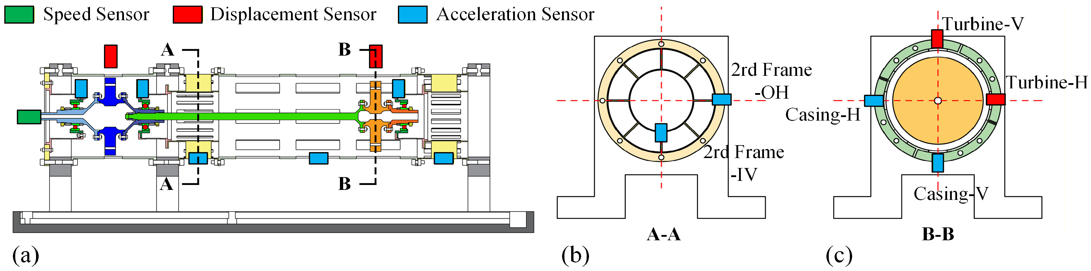
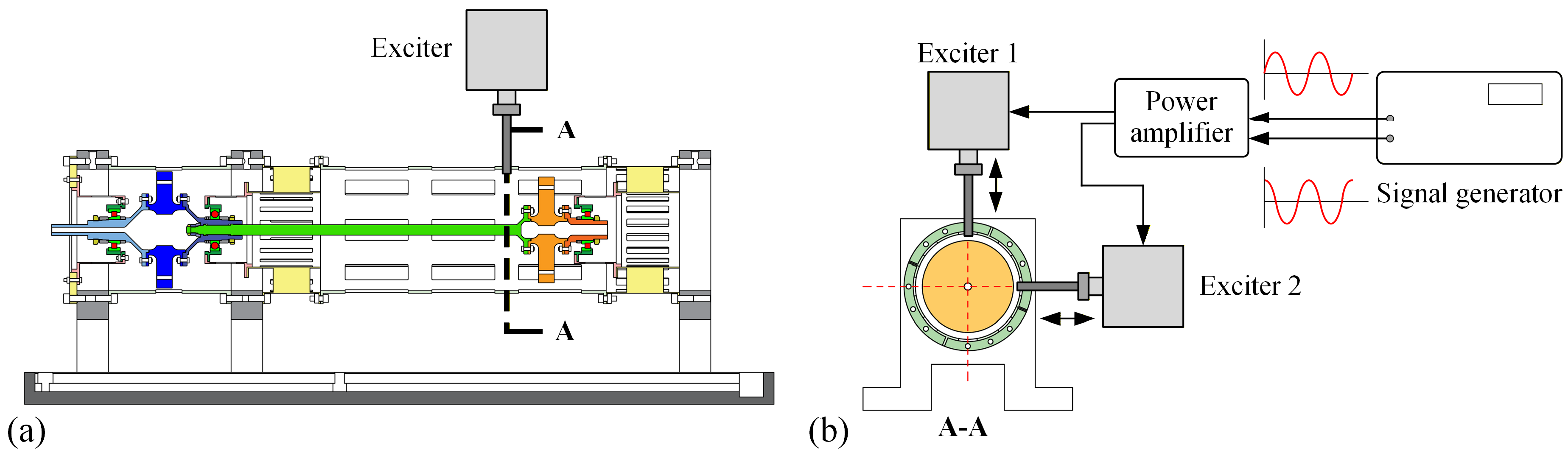
In order to realize effective vibration monitoring, multiple sensors were arranged at different positions of the test rig as shown in Figure 21. Among them, a speed sensor was used to collect real-time rotational speed and was placed at the forefront of the rotor; the non-contact eddy current displacement sensors were used to collect the vibration signal of the rotor and were placed at Disk 1 and Disk 2. The acceleration sensors were used to collect the vibration signal of the stator and were placed at three bearings (the 1#, 2#, and 3# Supports), two frames (the 2# and 3# Frames), and the casing. At each position, sensors were all set up at vertical and horizontal positions, represented by “V” and “H”, and the phase relationship can be seen from the “A-A” and “B-B” profiles in Figure 21. In addition, two orthogonal exciters were applied at vertical and horizontal orientations in order to obtain the mode shape vectors of the rotor–stator system, as shown in Figure 22.

5.2. Experimental Validation of the Evaluation Method

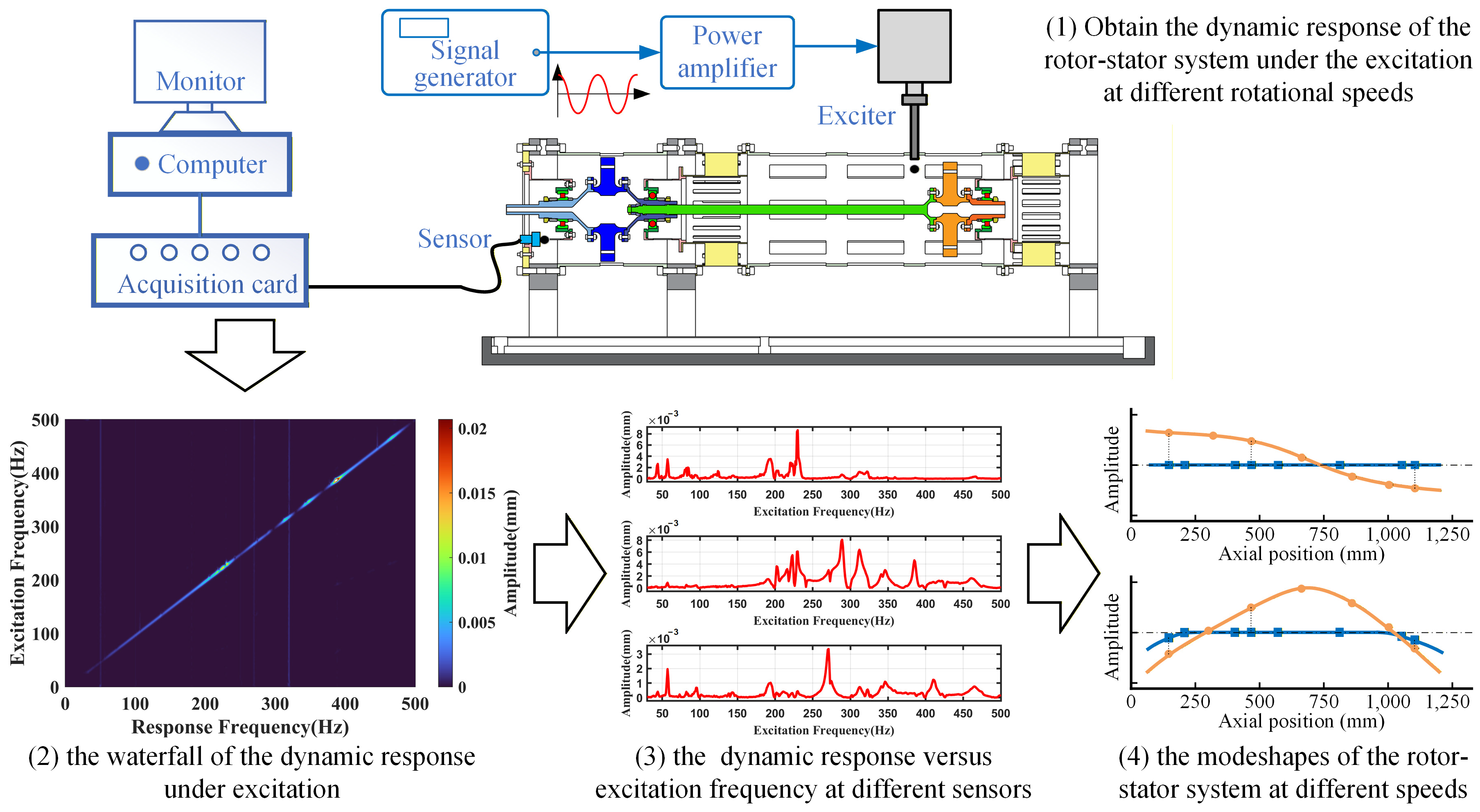
The evaluation method proposed earlier was validated through the experiments in this section. As derived from Equation (25), the core step of validation is how to obtain the mode shape vectors for both the rotor-only system and the rotor–stator system. The methodology is illustrated schematically in Figure 23 and Figure 24, respectively.

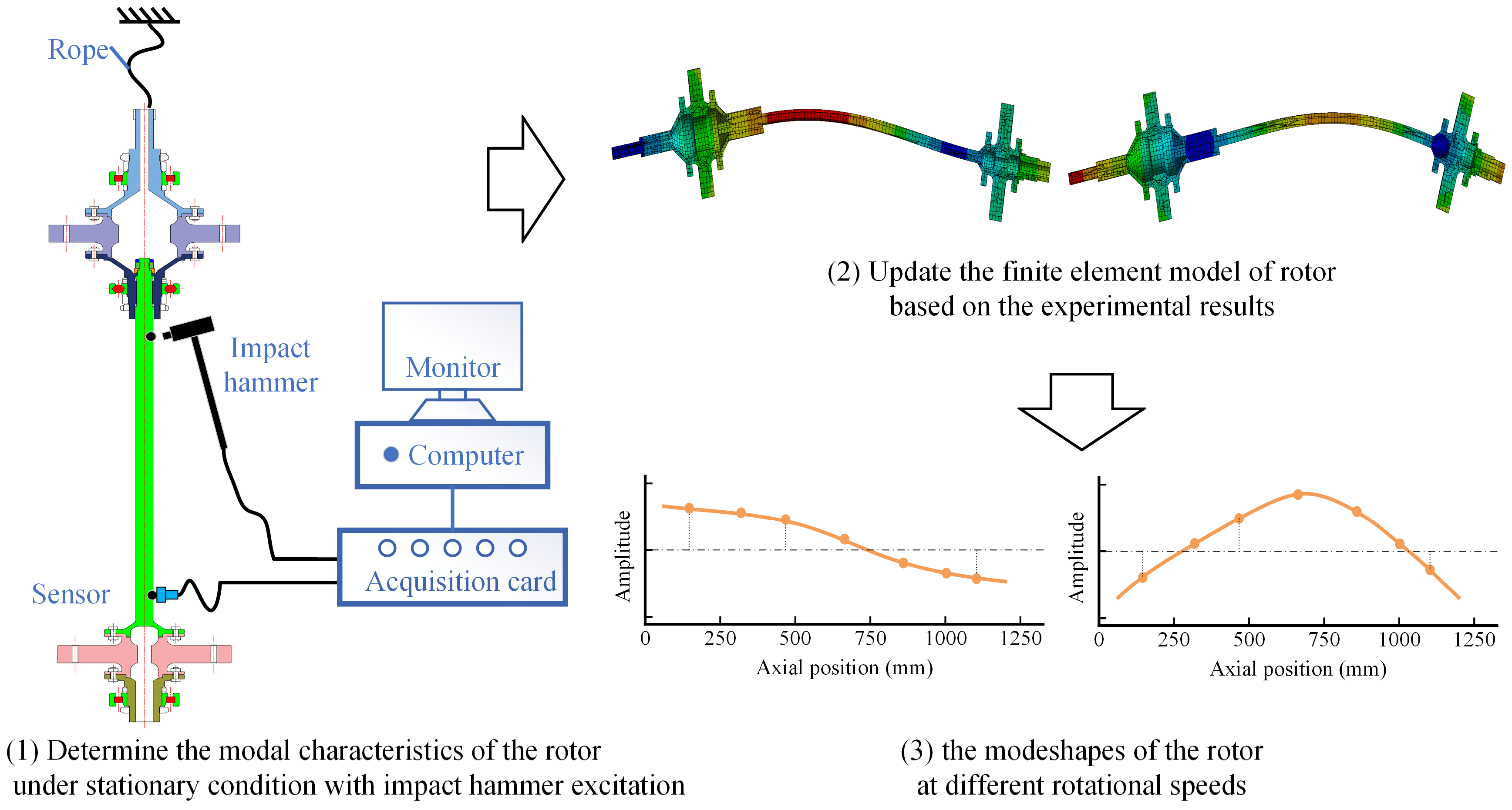
For the rotor-only system, the direct experimental measurement of the modal characteristics during rotating is infeasible due to practical constraints (e.g., the inability to isolate the rotor at operational speeds). To address this limitation, a hybrid experimental–numerical strategy was implemented as shown in Figure 23. (1) The impact hammer testing was first conducted to extract modal characteristics under stationary conditions. (2) The finite element model of the rotor was calibrated based on the experimental results. The bolted joint stiffness parameters in the rotor FE model were adjusted to match the modal characteristic calculation results with the experimental results. (3) The updated FE model simulated rotor dynamics versus rotational speeds generated speed-dependent modal shape vectors ${\mathit{u}}_r$. This approach effectively decouples gyroscopic effects from structural deformation modes, enabling accurate prediction of rotor dynamics.

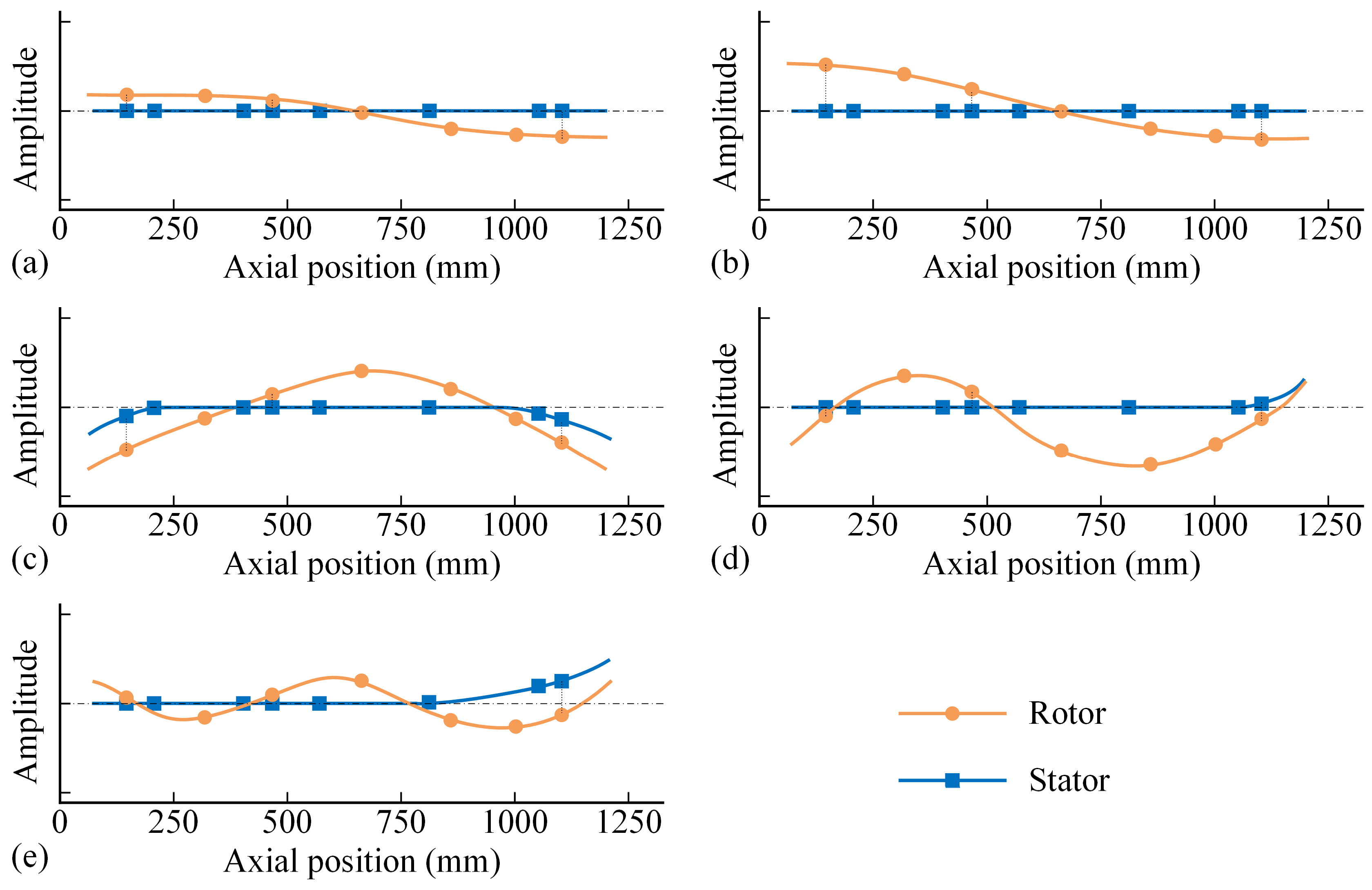
For the rotor–stator system, the impact hammer test was first used to identify the modal characteristics under stationary conditions. The mode shape vectors of the rotor–stator system under stationary conditions are shown in Figure 25.

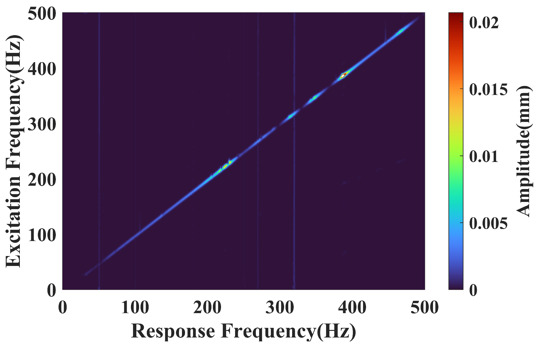
In addition, the mode shape vectors of the rotor–stator system under rotating conditions were equivalent to the dynamic response under the excitation of the exciters, as shown in Figure 24. (1) Two orthogonal exciters were applied at vertical and horizontal orientations, as shown in Figure 22. (2) In the experiment, the exciters applied swept-sine excitation (30~500 Hz range, 10 Hz/s sweep rate) while the rotor operated at constant rotational speeds and the combined responses (both the imbalance and excited response) were obtained. The dynamic response of Disk 2 under the excitation of the exciters at 3000 rpm is shown in Figure 26. (3) The imbalance-induced responses were subtracted from the combined responses, and the exciter-induced response was isolated. And the dynamic response versus the excitation frequency at different sensors can be obtained. (4) Response amplitudes and phases at identified resonant frequencies were synthesized across all measurement locations to construct mode shape vectors at each target speed ${\mathit{u}}_w$.

The mode shape vectors were experimentally characterized at rotational speeds ranging from 0 to 9000 rpm, with discrete intervals of 1000 rpm, enabling comprehensive validation of the evaluation method under realistic operating conditions.

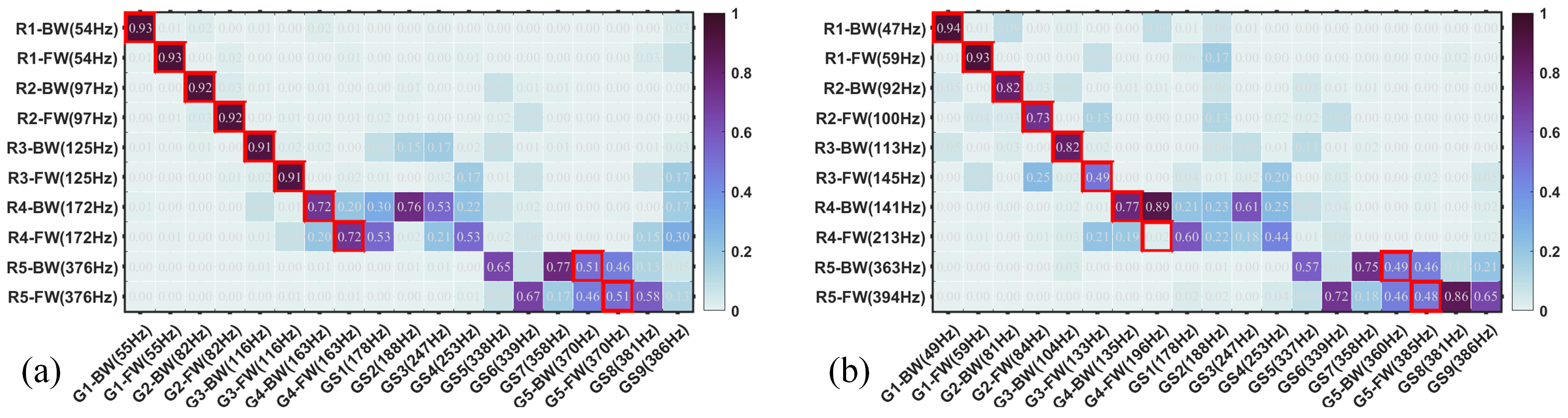
The MSCC distributions shown in Figure 27 were derived from experimental mode shape vectors. It can be seen from Figure 27 that the MSCCs of low-order rotor-dominated modes are generally higher and close to 1, while the MSCCs of the other modes are lower. There is a clear correspondence between the rotor-dominated modes of the rotor-only system and those of the rotor–stator system. It can be observed that there is significant similarity between Figure 17 and Figure 27. The high similarity between experimental and simulated MSCC distribution confirms the validity of the experimental operation process and data processing methodology, particularly in terms of the mode shape vector extraction accuracy.

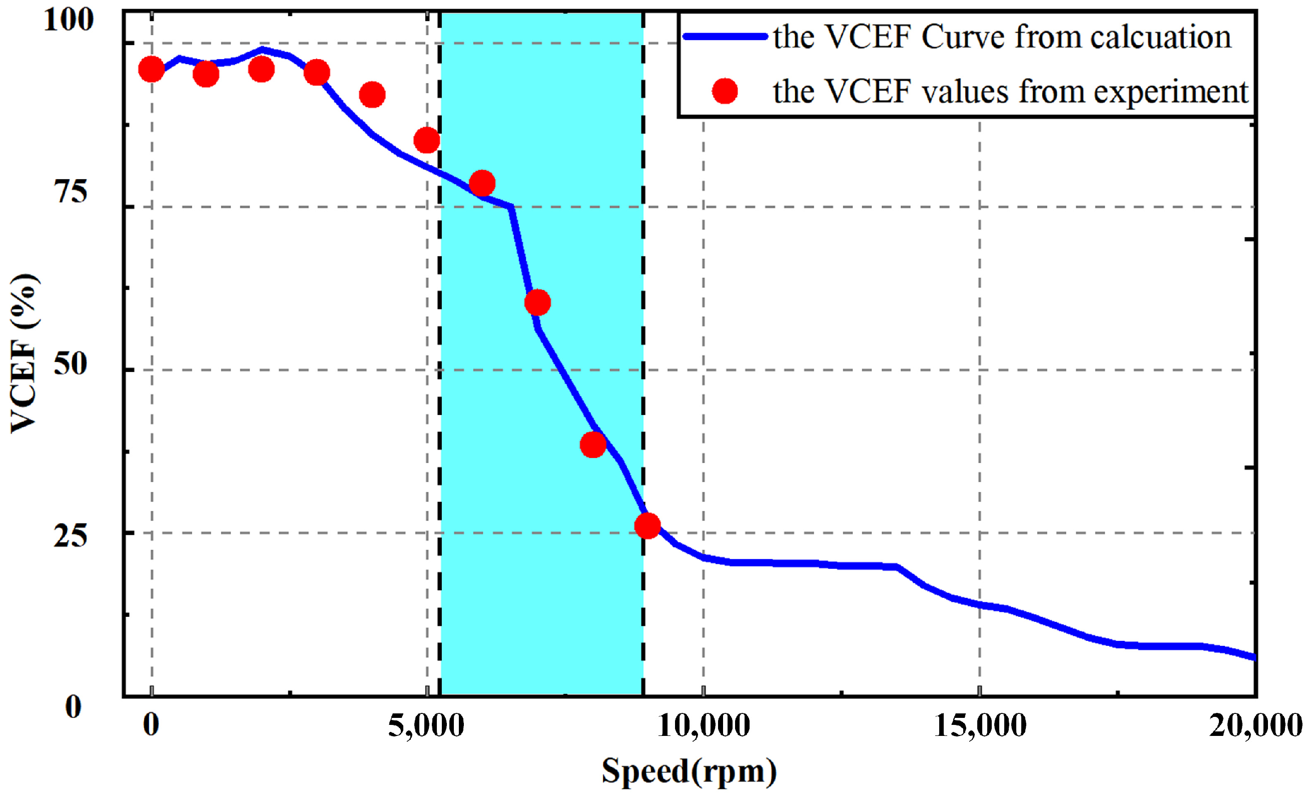
Based on the mode shape vectors of the rotor-only system and the rotor–stator system obtained from the experiment, the experimental VCEF values can be calculated based on Equation (25). The experiments covered rotational speeds ranging from 0 to 9000 rpm, with discrete intervals of 1000 rpm. Notably, measurements beyond 9000 rpm were infeasible due to the drive motor. Therefore, the experimental VCEF values at the testing rotational speeds were obtained and shown in Figure 28.

It can be seen from Figure 28 that the experimental VCEF values have a high degree of agreement with the simulation results, with an error of no more than 5%. Specifically, the experimental VCEF values generally show a monotonically decreasing trend as the rotational speed increases. Within 3000 rpm, the rotor operates at the subcritical state and there are few deformations of each stator-dominated mode shape. Therefore, the rotor–stator vibration coupling is weak and the experimental VCEF value is near to 1. The VCEF values stabilized above 0.75 in the range of 3000–6000 rpm and slightly decrease with the rotational speed, indicating slight rotor–stator vibration coupling within this rotational speed range. Within the scope of experimental rotational speeds, a rapid decrease in the experimental VCEF values can be identified in the range of 6000–9000 rpm, the light blue range shown in Figure 28, which is consistent with simulation results and previous analyses.

In Figure 19, there is also a rapid decrease in VCEF values within 13,500–16,000 rpm, indicating another enhancement of the rotor–stator vibration coupling. However, the rapid decrease phenomenon cannot be measured due to the limited experimental conditions.

In general, there is good consistency between the experimental results and the calculation results. Therefore, the existing experimental results have strongly validated the effectiveness of the quantitative evaluation method proposed in this paper.

6. Conclusions

This study proposes a novel evaluation method for rotor–stator vibration coupling in modern aeroengines. The proposed Vibration Coupling Evaluation Factor (VCEF), considering the similarity of the rotor-dominated modes between the rotor-only system and the rotor–stator system, provides a robust quantitative metric for rotor–stator vibration coupling. Through integrated theoretical modeling, numerical simulation, and experimental validation, the following key conclusions are drawn:

(1) The VCEF effectively captures the rotor–stator vibration coupling. In the low rotational speed range, the VCEF remains high, indicating weak vibration coupling. As the rotational speed increases, there will be stepped decreases in the VCEF values, signaling a significant increase in rotor–stator vibration coupling. Through the stepped decrease in the VCEF values, one can identify the rotational speed range where the dynamic response of the rotor–stator system is significantly different from that of the rotor-only system due to rotor–stator vibration coupling.

(2) The evaluation method is validated through both numerical simulations and experiments. Both the numerical simulations and experimental testing procedures of the proposed evaluation method were systematically investigated. The close agreement between numerical simulation and experimental results validates the accuracy and practical applicability of the VCEF for quantifying rotor–stator vibration coupling.

(3) The rotor–stator stiffness and mass distribution play a crucial role in determining the extent of vibration coupling. The sensitivity analysis of structural parameters was studied with the simple rotor–stator system, and the rotor–stator ratio of stiffness and mass significantly influences vibration coupling. In addition, there are few influences of the structure damping and the coupling stiffness on the VCEF values. By adjusting these parameters, engineers can optimize the design of aeroengine structures to mitigate undesirable dynamic effects and enhance system stability.

In summary, this study establishes a robust foundation for evaluating rotor–stator vibration coupling within the framework of the linear system, which delivers actionable engineering insight, enabling designers to determine when rotor–stator vibration coupling needs to be considered and researched. This transition from qualitative assessment to quantitative, speed-dependent criteria significantly enhances the fidelity and efficiency of dynamic analysis for high-speed rotating machinery. This method is not limited to aeroengines but is applicable to other high-speed rotating systems, delivering structural optimization guidance during the early design phase and enabling precise fault root cause identification in troubleshooting scenarios. Future research should focus on extending the method to the nonlinear system and exploring its implementation for real-time aeroengine health monitoring, which is an important and logical direction for future research.

References

1. Lin, R.; Hou, L.; Dun, S.; Cai, Y.; Sun, C.; Chen, Y. Synchronous Impact Phenomenon of a High-Dimension Complex Nonlinear Dual-Rotor System Subjected to Multi-Frequency Excitations. Sci. China Technol. Sci. 2023, 66, 1757–1768. [Google Scholar] [CrossRef]
2. Hong, J.; Liu, F.; Ma, Y.; Chen, X.; Wang, Y. Composite Failure Analysis of an Aero-Engine Inter-Shaft Bearing Inner Ring. Eng. Fail. Anal. 2024, 165, 108707. [Google Scholar] [CrossRef]
3. Zhong, Y.; Li, T.; Qu, S.; Huang, H.; Zhang, Z. Failure Analysis of Over-Temperature of Aero-Engine Bearing. J. Fail. Anal. Prev. 2023, 23, 1869–1879. [Google Scholar] [CrossRef]
4. Yu, P.; Wang, C.; Hou, L.; Chen, G. Dynamic Characteristics of an Aeroengine Dual-Rotor System with Inter-Shaft Rub-Impact. Mech. Syst. Signal Process. 2022, 166, 108475. [Google Scholar] [CrossRef]
5. Ma, Y.; Song, Z.; Yang, Z.; Li, C.; Ma, Y.; Hong, J. Research on the Dynamic Behavior of Rotor–Stator Systems Considering Bearing Clearance in Aeroengines. Actuators 2025, 14, 594. [Google Scholar] [CrossRef]
6. Cheli, F.; Cavalca, K.L.; Dedini, F.G.; Vania, A. Supporting Structure Effects on Rotating Machinery Vibrations. Vib. Rotating Mach. 1992, 6, 543–548. [Google Scholar]
7. De Santiago, O.; Abraham, E. Rotordynamic Analysis of a Power Turbine Including Support Flexibility Effects. In Proceedings of the GT2008, Berlin, Germany, 9 June 2008; Volume 5, pp. 1173–1181. [Google Scholar]
8. Zhang, D.Y.; Liu, Y.H.; Hong, J.; Ma, Y.H. Investigation on Dynamical Modeling and Vibration Characteristics for Aero Engine. Adv. Technol. (Tuijin Jishu) 2015, 36, 768–773. [Google Scholar]
9. Yu, M.; Feng, N.; Hahn, E.J. An Equation Decoupling Approach to Identify the Equivalent Foundation in Rotating Machinery Using Modal Parameters. J. Sound Vib. 2016, 365, 182–198. [Google Scholar] [CrossRef]
10. Yu, M.; Liu, J.; Feng, N.; Hahn, E.J. Experimental Evaluation of a Quasi-Modal Parameter Based Rotor Foundation Identification Technique. J. Sound Vib. 2017, 411, 165–192. [Google Scholar] [CrossRef]
11. Zhang, X.; Yang, Y.; Ma, H.; Shi, M.; Wang, P. A Novel Diagnosis Indicator for Rub-Impact of Rotor System via Energy Method. Mech. Syst. Signal Process. 2023, 185, 109825. [Google Scholar] [CrossRef]
12. Song, X.; Ren, Y.; Han, Q. Nonlinear Vibration of Rotating Cylindrical Shell Due to Unilateral Contact Induced Tip Rubbing Impact: Theoretical and Experimental Verification. Mech. Syst. Signal Process. 2022, 164, 108244. [Google Scholar] [CrossRef]
13. Ma, X.; Zhang, Z.; Hua, H. Uncertainty Quantization and Reliability Analysis for Rotor/Stator Rub-Impact Using Advanced Kriging Surrogate Model. J. Sound Vib. 2022, 525, 116800. [Google Scholar] [CrossRef]
14. Kang, Y.; Cao, S.; Hou, Y.; Chen, N.; Li, B. Dynamics Research on the Rubbing Process and Rubbing Forms of Rotor–Blade–Casing Systems. Int. J. Non-Linear Mech. 2022, 147, 104242. [Google Scholar] [CrossRef]
15. Zhu, Z.; Li, Y.; Wen, C.; Luo, Z.; Chen, Y.; Li, B. Rub-Impact Investigation of a Bolted Joint Rotor-Bearing System Considering Hysteresis Behavior at Mating Interface. Mech. Syst. Signal Process. 2025, 224, 112072. [Google Scholar] [CrossRef]
16. Zhang, Y.; Wang, S.; Zhao, K.; Xu, L.; Yang, F.; Li, Q. Vibration Characteristics of Dual-Rotor System with Staggered-Type Double Elastic Ring Squeeze Film Dampers under Maneuvering Flight. Aerosp. Sci. Technol. 2024, 152, 109351. [Google Scholar] [CrossRef]
17. Ye, J.; Wei, J.; Zhang, A.; Chen, S.; Ran, T.; Shu, R. Theoretical and Experimental Study on the Dynamic Behavior of Spur Gear Transmission System during Hovering Maneuver Flights. Mech. Syst. Signal Process. 2024, 212, 111296. [Google Scholar] [CrossRef]
18. Lu, K.; Guo, D.; Zhu, W.; Jin, Y.; Cheng, H.; Gu, X.; Fu, C. Nonlinear Dynamic Behavior Analysis of Dual-Rotor-Bearing Systems with Looseness and Rub–Impact Faults. AIAA J. 2023, 61, 5164–5175. [Google Scholar] [CrossRef]
19. Parent, M.-O.; Thouverez, F.; Chevillot, F. Whole Engine Interaction in a Bladed Rotor-to-Stator Contact. In Proceedings of the Volume 7A: Structures and Dynamics—American Society of Mechanical Engineers, Düsseldorf, Germany, 16 June 2014; p. V07AT31A003. [Google Scholar]
20. Wang, N.; Liu, C.; Jiang, D. Prediction of Transient Vibration Response of Dual-Rotor-Blade-Casing System with Blade Off. Proc. Inst. Mech. Eng. Part G J. Aerosp. Eng. 2019, 233, 5164–5176. [Google Scholar] [CrossRef]
21. Liu, J.; Fei, Q.; Wu, S.; Tang, Z.; Zhang, D. Nonlinear Vibration Response of a Complex Aeroengine under the Rubbing Fault. Nonlinear Dyn. 2021, 106, 1869–1890. [Google Scholar] [CrossRef]
22. Zhou, J.; Luo, Z.; Li, L.; Ma, T.; Li, H. Numerical and Experimental Analysis of the Influence of Elastic Supports on Bearing-Rotor Systems. Mech. Syst. Signal Process. 2025, 224, 112235. [Google Scholar] [CrossRef]
23. Dai, P.; Liang, X.; Li, J.; Wu, D.; Wang, F. Modeling Strategy and Mechanism Analysis for the Dual-Rotor-Disc-Bearing Coupled System with Unbalance Effect in Aeroengines. Mech. Syst. Signal Process. 2025, 224, 112086. [Google Scholar] [CrossRef]
24. Wang, W.; Wang, J.; Li, Q.; Li, W.; Wang, W. Investigation on the Dynamic Characteristics of a Rotor-Damper-Casing Coupling System under Diving-Climbing Maneuver. J. Sound Vib. 2024, 570, 118094. [Google Scholar] [CrossRef]
25. Luo, Z.; Zhou, J.; Li, L.; Sun, K.; Li, H. An Analytical Method of Dynamic Stiffness of Combined Supporting Structure and Its Effects on Rotor Systems: Simulation and Experiment. Int. J. Non-Linear Mech. 2024, 163, 104758. [Google Scholar] [CrossRef]
26. Li, L.; Luo, Z.; Liu, K.; Zhou, J. Dynamic Stiffness Characteristics of Aero-Engine Elastic Support Structure and Its Effects on Rotor Systems: Mechanism and Numerical and Experimental Studies. Appl. Math. Mech. 2023, 44, 221–236. [Google Scholar] [CrossRef]
27. Xu, H.; Ma, H.; Wen, B.; Yang, Y.; Li, X.; Luo, Z.; Han, Q.; Wen, B. Dynamic Characteristics of Spindle-Bearing with Tilted Pedestal and Clearance Fit. Int. J. Mech. Sci. 2024, 261, 108683. [Google Scholar] [CrossRef]
28. Guan, H.; Wang, P.; Xiong, Q.; Ma, H.; Zhou, S.; Mu, Q.; Zeng, Y.; Chen, Y. Modeling of Misaligned Bearing Induced by Coupling Misalignment and Assembly Errors and Vibration Analysis in Dual-Rotor System. Mech. Syst. Signal Process. 2025, 230, 112656. [Google Scholar] [CrossRef]
29. Tao, Y.; Tohti, G.; He, H.; Geni, M. Study on the Dynamic Optimization and Design of a Flexible Rotationally Symmetric Tangential Support Plate Base. Appl. Sci. 2025, 15, 2554. [Google Scholar] [CrossRef]
30. Ehehalt, U.; Alber, O.; Markert, R.; Wegener, G. Experimental Observations on Rotor-to-Stator Contact. J. Sound Vib. 2019, 446, 453–467. [Google Scholar] [CrossRef]
31. Chipato, E.T.; Shaw, A.D.; Friswell, M.I.; Sánchez Crespo, R. Experimental Study of Rotor-Stator Contact Cycles. J. Sound Vib. 2021, 502, 116097. [Google Scholar] [CrossRef]
32. Hu, L.; Palazzolo, A. Solid Element Rotordynamic Modeling of a Rotor on a Flexible Support Structure Utilizing Multiple-Input and Multiple-Output Support Transfer Functions. J. Eng. Gas Turbines Power 2017, 139, 012503. [Google Scholar] [CrossRef]
33. Dewi, D.K.; Abidin, Z.; Budiwantoro, B.; Malta, J. Dimensional Analysis of a Rotor System through FRF Using Transfer Function and Finite Element Methods. J. Mech. Sci. Technol. 2020, 34, 1863–1870. [Google Scholar] [CrossRef]
34. Chen, Y.-S.; Cheng, Y.-D.; Yang, T.; Koai, K.-L. Accurate Identification of the Frequency Response Functions for the Rotor–Bearing–Foundation System Using the Modified Pseudo Mode Shape Method. J. Sound Vib. 2010, 329, 644–658. [Google Scholar] [CrossRef]
35. Cavalca, K.L.; Cavalcante, P.F.; Okabe, E.P. An Investigation on the Influence of the Supporting Structure on the Dynamics of the Rotor System. Mech. Syst. Signal Process. 2005, 19, 157–174. [Google Scholar] [CrossRef]
36. Cavalca, K.L.; Okabe, E.P. On the Analysis of Rotor-Bearing-Foundation Systems. In Symposium on Emerging Trends in Rotor Dynamics; Springer: Dordrecht, The Netherlands, 2011. [Google Scholar] [CrossRef]
37. Hai, P.M.; Bonello, P. An Impulsive Receptance Technique for the Time Domain Computation of the Vibration of a Whole Aero-Engine Model with Nonlinear Bearings. J. Sound Vib. 2008, 318, 592–605. [Google Scholar] [CrossRef]
38. Bonello, P.; Minh Hai, P. A Receptance Harmonic Balance Technique for the Computation of the Vibration of a Whole Aero-Engine Model with Nonlinear Bearings. J. Sound Vib. 2009, 324, 221–242. [Google Scholar] [CrossRef]
39. Yang, Y.; Ouyang, H.; Yang, Y.; Cao, D.; Wang, K. Vibration Analysis of a Dual-Rotor-Bearing-Double Casing System with Pedestal Looseness and Multi-Stage Turbine Blade-Casing Rub. Mech. Syst. Signal Process. 2020, 143, 106845. [Google Scholar] [CrossRef]
40. Fahy, F.J. Statistical Energy Analysis: A Critical Overview. Philos. Trans. R. Soc. Lond. Ser. A Phys. Eng. Sci. 1994, 346, 431–447. [Google Scholar] [CrossRef]
41. Petrone, G.; Melillo, G.; Laudiero, A.; De Rosa, S. A Statistical Energy Analysis (SEA) Model of a Fuselage Section for the Prediction of the Internal Sound Pressure Level (SPL) at Cruise Flight Conditions. Aerosp. Sci. Technol. 2019, 88, 340–349. [Google Scholar] [CrossRef]
42. Van der Linden, P.J.G.; Fun, J.K. Using Mechanical-Acoustical Reciprocity for Diagnosis of Structure Borne Sound in Vehicles. J. Phys. IV 1994, 4, C5-93–C5-96. [Google Scholar] [CrossRef][Green Version]
43. Kim, B.-L.; Jung, J.-Y.; Oh, I.-K. Modified Transfer Path Analysis Considering Transmissibility Functions for Accurate Estimation of Vibration Source. J. Sound Vib. 2017, 398, 70–83. [Google Scholar] [CrossRef]
44. Ma, Y.; Zhao, Q.; Zhao, W.; Liu, B.; Hao, L. Intrinsic Physical Relationships between Rotor Modal Shapes and Instantaneous Vibrational Energy Flow Transmission Characteristics: Theoretical and Numerical Analysis and Application. Chin. J. Aeronaut. 2020, 33, 3288–3305. [Google Scholar] [CrossRef]
45. Ma, Y.; Zhao, Q.; Zhang, K.; Xu, M.; Zhao, W. Analysis of Instantaneous Vibrational Energy Flow for an Aero-Engine Dual-Rotor–Support–Casing Coupling System. J. Eng. Gas Turbines Power 2020, 142, 51011. [Google Scholar] [CrossRef]
46. Chipato, E.T.; Shaw, A.D.; Friswell, M.I. Nonlinear Rotordynamics of a MDOF Rotor–Stator Contact System Subjected to Frictional and Gravitational Effects. Mech. Syst. Signal Process. 2021, 159, 107776. [Google Scholar] [CrossRef]
47. Mikota, G.; Mikota, J. Energy Related Model Correlation Criteria for Modal Analysis of Fluid-Structure Interaction Systems. J. Sound Vib. 2020, 483, 115480. [Google Scholar] [CrossRef]
48. Mikota, G.; Manhartsgruber, B.; Brandl, A.; Treml, P. A Modal Method for Detection and Exclusion of Interactions. J. Sound Vib. 2023, 546, 117408. [Google Scholar] [CrossRef]
49. Guo, X.; Zeng, J.; Ma, H.; Zhao, C.; Yu, X.; Wen, B. A Dynamic Model for Simulating Rubbing between Blade and Flexible Casing. J. Sound Vib. 2020, 466, 115036. [Google Scholar] [CrossRef]
50. Yang, Z.; Hong, J.; Wang, D.; Cheng, R.; Ma, Y. Vibration Analysis of Rotor Systems with Bearing Clearance Using a Novel Conformal Contact Model. Nonlinear Dyn. 2024, 112, 7951–7976. [Google Scholar] [CrossRef]
51. Yu, P.; Jiang, Z.; Tao, X.; Li, S.; Jiang, K. Research on Lateral–Torsional Coupled Vibration Induced by Substantial Imbalance in an Overhung Flexible Rotor. Int. J. Non-Linear Mech. 2025, 169, 104959. [Google Scholar] [CrossRef]
52. De Paula, E.H.; De Castro, H.F. Effect of Gear Tooth Root Crack on the Dynamic Response of a Planetary Geared Rotor System. Mech. Mach. Theory 2025, 209, 105970. [Google Scholar] [CrossRef]
53. Mikota, G.; Brandl, A.; Treml, P. Modal Testing and Model Correlation of a Lumped Parameter Vibroacoustical System. In Proceedings of the International Conference on Noise and Vibration Engineering, Leuven, Belgium, 7–9 September 2020; pp. 1789–1803. [Google Scholar]
54. Zhang, X.; Wang, Y.; Chen, W.; Jiang, X. Parametric Study on the Flutter Sensitivity of a Wide-Chord Hollow Fan Blade. Chin. J. Aeronaut. 2022, 35, 277–293. [Google Scholar] [CrossRef]
55. Pastor, M.; Binda, M.; Harčarik, T. Modal Assurance Criterion. Procedia Eng. 2012, 48, 543–548. [Google Scholar] [CrossRef]
56. Mikota, G. A Model Correlation Criterion for Rotors. J. Sound Vib. 2019, 441, 106–110. [Google Scholar] [CrossRef]
57. Rajagopal, A.; Mandal, D.K. An Evaluation of Mode Tracking Methods for Practical Rotor Dynamic Analysis. In Proceedings of the Volume 7B: Dynamics, Vibration, and Control—American Society of Mechanical Engineers, Virtual, 16 November 2020. [Google Scholar]
Figure 1. Abstract expression of rotor–stator in aeroengine. The interaction between rotor, bearings, and stator results in vibration coupling.
Actuators 15 00019 g001
Figure 2. The coupling relationship in the parameter matrix.
Actuators 15 00019 g002
Figure 3. Schematic of the mode shape vector rotation.
Actuators 15 00019 g003
Figure 4. Flow chart of the quantitative evaluation method.
Actuators 15 00019 g004
Figure 5. Schematic of the example model.
Actuators 15 00019 g005
Figure 6. Campbell diagram of the example model: (a) the rotor system; (b) the rotor–stator system. At around 2700 rpm, the frequency of the 4th mode is approximately equal to that of the 5th and 6th modes, corresponding to the mode shape transformation.
Actuators 15 00019 g006
Figure 7. The mode shapes of the 4th, 5th, and 6th modes at (a) low speeds (<2300 rpm) and (b) high speeds (>2800 rpm): the mode shape of (a.1) the 4th mode at low speeds; (a.2) the 5th mode at low speeds; (a.3) the 6th mode at low speeds; (b.1) the 4th mode at high speeds; (b.2) the 5th mode at high speeds; (b.3) the 6th mode at high speeds.
Actuators 15 00019 g007
Figure 8. The MSCC distribution at different rotational speeds: (a) 0 rpm; (b) 2500 rpm; (c) 5000 rpm. There is an obvious one-to-one correspondence between the first four mode shapes at 0 rpm, and the similarity gradually diminishes as the rotational speed increases.
Actuators 15 00019 g008
Figure 9. The variation in VCEF versus rotational speed: The blue line represents the VCEF curve, the orange lines represent the mode frequency lines, and the red line represents the synchronous speed line of the Campbell diagram. The VCEF values dropped rapidly in the light blue range.
Actuators 15 00019 g009
Figure 10. The MSCC distributions during the drop of VCEF: (a) 2400 rpm; (b) 2600 rpm; (c) 2800 rpm. Due to the mode shape transformation, the MSCC (w,4,4) decreases significantly with significant increase in the MSCC (w,6,4).
Actuators 15 00019 g010
Figure 11. The influence of different parameters on VCEF: (a) the structural damping; (b) the coupling stiffness; (c) the rotor–stator stiffness ratio; (d) the stator mass. The VCEF values versus rotational speed under different values of specified parameters. It can be observed that the stiffness ratio and stator mass have significant influences on the VCEF curve at different rotational speeds, while the effects of structural damping and coupling stiffness are small.
Actuators 15 00019 g011
Figure 12. Schematic diagram of a certain type of high-thrust-to-weight-ratio turbofan engine.
Actuators 15 00019 g012
Figure 13. Schematic of the rotor–stator system.
Actuators 15 00019 g013
Figure 14. Schematic of finite element model for the rotor–stator system.
Actuators 15 00019 g014
Figure 15. Campbell diagram: (a) the rotor–stator system; (b) the rotor system.
Actuators 15 00019 g015
Figure 16. The mode shapes of the rotor system and the rotor–stator system: (a) R1 and G1; (b) R2 and G2; (c) R3 and G3; (d) R4 and G4; (e) R5 and G5. There is an obvious one-to-one correspondence between the mode shapes. However, there are deformations at the stator in the rotor-dominated mode shapes.
Actuators 15 00019 g016
Figure 17. The MSCC distribution at 0 rpm. There is a correspondence between the rotor-dominated modes of the two systems, which are circled in red boxes. The MSCCs of low-order rotor-dominated modes are generally higher close to 1, while the others are lower.
Actuators 15 00019 g017
Figure 18. The MSCC distribution at different rotational speeds: (a) 3000 rpm, (b) 6000 rpm, (c) 9000 rpm, (d) 12,000 rpm. There is a correspondence between the rotor-dominated modes of the two systems, which are circled in red boxes. As the rotational speed increases, the correspondence between the rotor-dominated modes significantly weakens and the MSCC values corresponding to each rotor-dominated mode significantly decrease.
Actuators 15 00019 g018
Figure 19. The variation in VCEF versus rotational speed: variation in VCEF with rotational speed. The blue line represents the VCEF curve, the orange lines represent the mode frequency lines, and the red line represents the synchronous speed line of the Campbell diagram. The VCEF values dropped rapidly in the light blue range.
Actuators 15 00019 g019
Figure 20. The rotor–stator system: (a) the schematic; (b) the test rig.
Actuators 15 00019 g020
Figure 21. The schematic of the signal collector: (a) distribution of sensors; (b) the A-A section; (c) the B-B section.
Actuators 15 00019 g021
Figure 22. Schematic diagram of the exciters in the tester: (a) distribution of exciters; (b) the A-A section.
Actuators 15 00019 g022
Figure 23. Schematic diagram of the mode shape vectors of the rotor-only system obtained from the experiment.
Actuators 15 00019 g023
Figure 24. Schematic diagram of the mode shape vectors of the rotor–stator system obtained from the experiment.
Actuators 15 00019 g024
Figure 25. The mode shape vectors of the rotor–stator system under stationary conditions with impact hammer excitation: (a) the 1st mode; (b) the 2nd mode; (c) the 3rd mode; (d) the 4th mode; (e) the 5th mode.
Actuators 15 00019 g025
Figure 26. The waterfall of the dynamic response under exciter at 3000 rpm.
Actuators 15 00019 g026
Figure 27. The MSCC distribution obtained from the experiment at (a) 0 rpm and (b) 3000 rpm.
Actuators 15 00019 g027
Figure 28. The variation in VCEF versus rotational speed obtained from the experiment: The blue line represents the VCEF curve, and the red dots represent the VCEF values calculated based on the experimental data. The VCEF values dropped rapidly in the light blue range.
Actuators 15 00019 g028
Disclaimer/Publisher’s Note: The statements, opinions and data contained in all publications are solely those of the individual author(s) and contributor(s) and not of MDPI and/or the editor(s). MDPI and/or the editor(s) disclaim responsibility for any injury to people or property resulting from any ideas, methods, instructions or products referred to in the content.