Intelligent Fault Diagnosis for Rotating Machinery via Transfer Learning and Attention Mechanisms: A Lightweight and Adaptive Approach

Abstract

Fault diagnosis under variable operating conditions remains challenging due to the limited adaptability of traditional methods. This paper proposes a transfer learning-based approach for bearing fault diagnosis across different rotational speeds, addressing the critical need for reliable detection in changing industrial environments. The method trains a diagnostic model on labeled source-domain data and transfers them to unlabeled target domains through a two-stage adaptation strategy. First, only the source-domain data are labeled to reflect real-world scenarios where target-domain labels are unavailable. The model architecture combines a convolutional neural network (CNN) for feature extraction with a self-attention mechanism for classification. During source-domain training, the feature extractor parameters are frozen to focus on classifier optimization. When transferring to target domains, the classifier parameters are frozen instead, allowing the feature extractor to adapt to new speed conditions. Experimental validation on the Case Western Reserve University bearing dataset (CWRU), Jiangnan University bearing dataset (JNU), and Southeast University gear and bearing dataset (SEU) demonstrates the method’s effectiveness, achieving accuracies of 99.95%, 99.99%, and 100%, respectively. The proposed method achieves significant model size reduction compared to conventional TL approaches (e.g., DANN and CDAN), with reductions of up to 91.97% and 64%, respectively. Furthermore, we observed a maximum reduction of 61.86% in FLOPs consumption. The results show significant improvement over conventional approaches in maintaining diagnostic performance across varying operational conditions. This study provides a practical solution for industrial applications where equipment operates under non-stationary speeds, offering both computational efficiency and reliable fault detection capabilities.

1. Introduction

Rotating machinery (e.g., bearings, gears, and turbines) serves as the cornerstone of modern industrial systems, whose operational reliability directly impacts productivity and safety [1]. However, under complex working conditions involving variable speeds and fluctuating loads, mechanical components are particularly prone to progressive wear, surface cracks, or mass imbalances—degradation patterns that often culminate in catastrophic failures if undetected [2]. While traditional vibration-based monitoring methods have formed the backbone of condition monitoring for decades, their heavy reliance on expert-designed features (e.g., kurtosis, envelope spectra) and physics-based models presents fundamental limitations [3]. As demonstrated by recent studies, these conventional approaches exhibit poor generalization capability when confronted with unseen operational scenarios or novel fault types, primarily due to their inherent dependence on prior domain knowledge and static diagnostic rules [4]. For instance, methods based on Hilbert–Huang transform (HHT), though effective in some cases, struggle with endpoint effects and require manual feature engineering, making them less adaptable to dynamic industrial environments [5]. This knowledge gap becomes particularly pronounced in modern industrial settings where equipment operates under increasingly variable conditions, exposing a critical need for more adaptive diagnostic paradigms that can automatically extract discriminative features from raw vibration signals [6].

With the advent of deep learning, data-driven fault diagnosis techniques, particularly convolutional neural networks (CNNs), have demonstrated superior capability in automatic feature extraction, overcoming the limitations of manual feature engineering in traditional vibration analysis methods [7]. These deep learning approaches excel at learning hierarchical representations directly from raw vibration signals, enabling more robust fault diagnosis across various mechanical components such as bearings [8] and gears [9]. However, despite these advancements, two critical bottlenecks persist in practical industrial applications. First, the issue of data scarcity remains challenging, as labeled fault samples from real-world industrial equipment are extremely limited due to the high costs and risks associated with collecting fault data from operational machinery [10]. This scarcity is particularly problematic given that training deep models typically requires massive annotated datasets to achieve satisfactory generalization performance. Second, the problem of domain shift significantly impacts model reliability, where diagnostic models trained under controlled laboratory conditions often experience severe performance degradation when deployed to field environments [11]. This degradation stems from distribution discrepancies in key operational factors such as noise levels, varying loads, and rotational speeds between source and target domains [12]. Recent studies have shown that even state-of-the-art CNNs architectures can suffer from accuracy drops when facing such domain shifts in real-world scenarios [13].

The above limitations greatly limit the universality and reliability of fault diagnosis methods in complex and ever-changing industrial environments. Therefore, it is particularly important to establish a fault diagnosis system that can adapt to multiple working conditions and scenarios. While transfer learning (TL) has emerged as a promising solution to address domain adaptation by leveraging knowledge from labeled source domains, current TL-based diagnosis frameworks still face three unresolved challenges that hinder their practical deployment:

• Over-parameterization: Most TL models inherit cumbersome architectures, hindering edge-device deployment.
• Attention Mechanism Limitations: Existing attention modules (e.g., SE, CBAM) introduce excessive parameters or fail to capture cross-scale fault features effectively.
• Dynamic Adaptation: Few methods consider the real-time variability of mechanical signals, leading to suboptimal performance under non-stationary conditions.

To bridge these gaps, this study proposes a lightweight yet adaptive fault diagnosis framework by synergizing parameter-efficient TL with advanced attention mechanisms. Our key contributions include the following:

• Propose a lightweight CNN self attention feature extractor that reduces parameter overhead. (Our method demonstrates a superior performance compared to DANN and CDAN, reducing model size by 91.97% and 64.83%, respectively.) In addition, it effectively enhances discriminative feature learning, particularly under variable speed conditions.
• Design a pseudo-label domain adaptation strategy for transfer learning in response to distribution shifts caused by changes in rotational speed.
• Experimental validation on the CWRU, JNU, and SEU datasets, showing % higher accuracy than state-of-the-art methods under variable noise levels.

The remainder of this paper is organized as follows: Section 2 reviews related work; Section 3 details the proposed methodology; Section 4 presents experiments and discusses the experimental results; and Section 5 concludes the study.

2. Related Work on TL for Rotating Machinery

In this section, relevant methods such as domain adaptation methods, adversarial transfer learning, and pre-training strategies will be discussed and studied.

2.1. Statistical Alignment Based Method

In terms of statistical alignment based methods (e.g., MMD and Coral), Li et al. [14] proposed a deep TL model using Coral [15] and MMD [16] methods to analyze fault data for the diagnosis of spray pump faults. By analyzing three different types of faults in the spray pump under variable operating conditions, the diagnostic accuracy could reach an average of 90%. Zhang et al. [17] used short-time Fourier transform and a deep residual network to convert the one-dimensional signal of motor bearings into a two-dimensional time–frequency map and then conducted transfer training through Resnet. The accuracy in the CWRU bearing dataset reached an average accuracy of 98.96%. To address the challenge of correctly aligning covariance matrices within a manifold structure, Cui et al. [18] proposed an improved domain alignment method called LD-CORAL. This method utilizes the Log-Euclidean distance to calculate the deep CORAL loss, thereby enhancing the model’s feature learning capability. It achieved an average accuracy of 98.8% on the CWRU dataset. An et al. [19] used cross-entropy loss to select the error between the true class of the sample and the predicted results. Their model achieved an average accuracy of over 97.46% in six groups of transfer learning fault diagnosis. Ding et al. [20] proposed a novel prediction architecture entitled as a statistical alignment-based metagated recurrent unit. Its effectiveness was verified using FEMTO-ST bearing datasets and industrial datasets. Chen et al. [21] pointed out that the existing multi-source transfer diagnosis models for gearboxes have limited generalization ability in different transfer tasks while ignoring the influence of feature distribution differences between the target domain and each source domain on the model. By constructing an auxiliary domain alignment module based on MMD, its accuracy could reach 93.5% in gearbox multi-source data diagnosis tasks. Kim et al. [22] achieved accuracy rates of 60.7% and 73.85% on the CWRU and Paderborn (PU) datasets, respectively. Using CNN as the backbone network in combination with MK-MMD as the domain alignment method, Xiao et al. [23] tackled the problem of data distribution shifts in fault scenarios by proposing a domain adaptation module employing multi-kernel local maximum mean discrepancy (MK-LMMD) for distribution alignment. Their method achieved an average accuracy of over 98% in cross-domain transfer learning experiments on three bridge datasets. Overall, statistical alignment methods show great potential in rotating machinery fault diagnosis, and they can improving model accuracy and generalization.

2.2. Adversarial Generative-Based Method

In terms of adversarial generative methods, Zhang et al. [24] utilized deep adversarial networks to address challenges posed by domain shift and data privacy. Their experiments demonstrated impressive accuracy, exceeding 91% on the train bogie dataset and 97% on the CWRU dataset. Zhang et al. [25] applied the model built on the CWRU bearing dataset to the Southeast University gearbox bearing dataset, and the experimental results showed that the accuracy reached 100%. Farag et al. [26] found through experiments that combining the conditional domain adversarial network (CDAN) transfer learning method improved performance by 21.6% and 26.9% on the CWRU and PU datasets, respectively, compared to just using the MMD. Tang et al. [27] conducted cross-domain fault diagnosis analysis on CWRU and JNU (Jiangnan University Bearing Dataset) using generative adversarial networks, with an average accuracy rate exceeding 84%. Alasmer et al. [28] proposed a CNN knowledge transfer model based on VGG-19 to address the heterogeneity of sensor data and reduce the cost of human intervention. The experimental results revealed that this model achieved a classification accuracy of 99.8% for bearing faults. Zhu et al. [29] proposed an advanced Wasserstein generative adversarial network (WGAN) method to diagnose bearing faults by generating time–frequency images through continuous wavelet transforms. They achieved high diagnostic accuracy rates of 98.9% and 97.4% on the CWRU and centrifugal pump datasets while reducing dependence on labeled data. Shakiba et al. [30] used TL methods to transfer fault knowledge accumulated in other devices or similar systems to the target power system, thereby improving the accuracy and efficiency of fault detection and diagnosis. Wang et al. [31] achieved an average accuracy of 94.99% on the CWRU dataset by domain adversarial neural networks (DANNs) with TL. To tackle the issue of imbalanced samples, Liu et al. [32] proposed an approach utilizing coupled generative adversarial networks (CoGANs). Their method achieved a remarkable 100% accuracy on the CWRU dataset. These studies demonstrate that adversarial generative models hold significant potential for enhancing fault diagnosis accuracy, generalization, and efficiency.

2.3. Pre-Training Strategies

In terms of pre-training, due to the complexity of multi-layer network architectures, the issue of overfitting can easily arise, thereby affecting the generalization ability of the model. Therefore, pre-training strategies are crucial. Inspired by greedy algorithms, Zhao et al. [33] adopted a shallow supervised network to pre-train the weights of denoising layers, thus reducing the difficulty of model training. This approach achieved an accuracy of 95.32% in fault diagnosis for wind turbine gearbox systems. To address the challenge of scarce target-domain data, Wu et al. [34] proposed a Transformer-based Transfer Learning Network (TTLN). This model extracts fault features during the pre-training phase and then fine-tunes and updates a subset of its parameters during target-domain training, thereby mitigating the impact of model drift. It achieved an accuracy exceeding 95% on both the CWRU and PU datasets. Asukar et al. [35] adjusted the parameters (i.e., weights and biases) in the CNN convolutional layer and reduced the loss between the target domain and the source domain by 5% through re-training. Yan et al. [36] proposed using synthetic data during the pre-training phase of transfer learning to expand the training dataset and reduce the need for manual annotation. When processing vibration signals, Maggio et al. [37] adopted a pre-training method of classifying audio data first and then implemented TL through knowledge transfer techniques to perform fault diagnosis. To mitigate the high cost of pre-training, Chakraborty et al. [38] proposed efficient filtering methods to select relevant subsets from the pre-training dataset. They found that this approach effectively balanced cost and performance and could even improve the pre-training benchmark by 1–3%. Due to the need for sufficient labeled data in traditional fault diagnosis methods, Sandeep et al. [39] proposed using multi-level kurtosis fusion for TL, which can effectively reduce the time required for knowledge transfer. Pei et al. [40] enhanced the performance of a transfer learning-based fault diagnosis model during its pre-training phase. They employed reverse propagation of the target-domain training data to fine-tune the pre-trained model, thereby improving its accuracy. The model achieved accuracies of 99.71%, 99.97%, and 99.83% on the CWRU, UPB, and SEG datasets, respectively. These pre-training strategies address the challenges of transfer learning by optimizing initialization, leveraging diverse data sources, simplifying training, and integrating target domain information, ultimately boosting diagnostic accuracy and generalization ability.

3. Materials and Methods

In real-world industrial scenarios, significant variations in operating conditions (e.g., rotational speed, load, and position. Here, “position” refers to the spatial location or orientation of components in the mechanical system. For instance, in a rotating machinery setup, the position could denote the specific angular placement of a rotor relative to the stator or the linear position of a sliding part in a mechanical structure. These variations in position can lead to changes in the mechanical interactions and vibration characteristics, thus affecting the fault signals and making fault diagnosis more complex) cause the distribution and patterns of fault signals to vary across different conditions, making models trained on a single condition difficult to generalize effectively [41]. Traditional machine learning and deep learning methods typically require extensive labeled data from multiple conditions for training. However, in practical applications, data collection is costly, and labeled data under different conditions are often scarce [42]. Therefore, TL strategies offer an effective solution to reduce the reliance on labeled data [43].

To address these challenges, this paper proposes a TL-based fault diagnosis method for variable operating conditions. As shown in Figure 1, the approach first pre-trains a self-attention model on a single condition (source domain) to establish initial fault classification capability. Then, a TL strategy is applied to adapt the trained self-attention model parameters to the target domain. The model is further enhanced by integrating a CNN for feature extraction, followed by joint optimization on the target domain data to ensure adaptation to new operating conditions.

3.1. Dataset Partitioning for Source and Target Domains in TL

In the context of TL, it is essential to partition the source-domain and target-domain datasets. The source domain is defined under the condition of labeled data, and its formal definition is given as follows:

$$D_s={\left\{(x_i^s,y_i^s)\right\}}_{i=1}^{n_s},x_i^s\in X_s,y_i^s\in Y_s$$

(1)

where $D_s$ represents the source-domain dataset, $x_i^s\in {\mathbb{R}}^d$ is the i-th sample, $X_s$ is the set of all samples, $y_i^s$ is the set of all distinct labels, and $n_s$ denotes the total number of source samples. Consequently, the target domain is defined as

$$D_t={\left\{\left(x_i^t\right)\right\}}_{i=1}^{n_t},x_i^t\in X_t$$

(2)

In this case, $D_t$ represents the target-domain dataset, $x_i^t\in {\mathbb{R}}^d$ is the i-th sample, $X_t$ is the set of all target samples, and $n_t$ denotes the total number of target samples.

The label distribution probabilities of the source domain and the target domain are represented by P and Q, respectively. Using the formula $\widehat{y}=\beta \left(x\right)$, we can classify the unlabeled data x in the target domain, where $\widehat{y}$ is the predicted distribution. Based on this, the difference ${ϵ}_t\left(\beta \right)$ between the target domain and source domain is aligned using the features of the source-domain data. The data partitioning formulas for the source domain are given below, where $\rho$ is the ratio of the random partition value:

$$|x_i^s|=\rho \times |{\mathcal{D}}_s|$$

(3)

$$|y_i^s|=(1-\rho )\times |{\mathcal{D}}_s|$$

(4)

The above formulas ensure that the source-domain data are used for training, which truly reflect the model’s performance on labeled data, while the target-domain data are left unlabeled to facilitate TL.

3.2. CNN–Attention Model

In this study, a CNN–Attention-based fault diagnosis model was constructed, which was trained using labeled source-domain data to learn the fault features of different categories (Normal, Ball, Inner race, Outer race). The model followed the structure and process outlined below:

1.

To improve training efficiency while ensuring accuracy, a lightweight CNNs feature extractor was designed. This lightweight design reduces computational complexity by employing a streamlined convolutional layer structure, which consequently reduces training time [44]. The structure achieves high accuracy while converging faster, significantly accelerating the training process.

The model extracts deeper features from the input raw signals and outputs them as feature vectors. The constructed model consists of two convolutional layers, each with two batch normalization layers to accelerate training efficiency and enhance generalization capability. Two ReLU activation functions enable the model to learn more complex feature relationships. The two convolution layers are Conv1 and Conv2 in Figure 1. Global average pooling is applied to obtain a feature vector from Conv2.

2.

The classifier model incorporates the self-attention mechanism to dynamically adjust the extracted features. This allows the model to focus more on the feature regions useful for classification, thereby enhancing detection performance. Given the feature vector Z as input, the input to the classifier is the feature vector, which is linearly transformed to obtain $\mathcal{Q}$ and K, as shown in Equations (5) and (6) below:

$$\mathcal{Q}=W_{q}Z$$

(5)

$$\mathcal{K}=W_{k}Z$$

(6)

where the input of the classifier is $\mathbb{R}$, and the feature vector is $\{ \in \mathbb{R}$.

Therefore, the attention weight coefficient is computed as

$$w=exp(\mathcal{Q}·\mathcal{K})/\sum exp({\mathcal{Q}}_i·{\mathcal{K}}_i)$$

(7)

Next, the feature vector is weighted using the attention weight coefficient:

$$f^{\prime }=\mathrm{w}\times f$$

(8)

$$y=W_{fc}{f}^{\prime }+b_{fc}$$

(9)

Finally, a fully connected layer outputs the logits for the 4 categories, which are used to identify fault types. The convolutional layers, linear layers, and batch normalization of the model are then initialized appropriately to ensure the stability of the training process.

Compared to Squeeze-and-Excitation (SE) and Convolutional Block Attention Module (CBAM), the scaled dot-product attention mechanism offers several advantages for fault diagnosis in rotating machinery. First, it dynamically captures long-range dependencies in vibration signals without introducing excessive parameters, which is critical for lightweight models. SE and CBAM, while effective in vision tasks, often fail to model cross-scale fault features efficiently due to their localized attention mechanisms. Second, the dot-product attention explicitly computes interactions between all feature positions, enabling the model to focus on discriminative fault patterns under variable speed conditions. This is particularly important for bearing faults, where fault signatures may span multiple frequency bands. Finally, the self-attention mechanism assigns adaptive weights to features according to their relevance to the fault type, which markedly diminishes the need for manual feature engineering and overcomes a principal shortcoming of traditional methods.

3.3. Loss Function and Fine-Tuning Strategy

The core of TL lies in knowledge transfer from the source domain, combined with fine-tuning strategies to enhance the efficiency and effectiveness of model training in the target domain, addressing challenges from different operational conditions [45]. In this study, we adopted the cross-entropy loss function $\mathcal{L}$ as the classification strategy to enable knowledge transfer and classification alignment between the source and target domains. When applying deep learning models for fault diagnosis, the model’s output class probabilities are transformed via the Softmax function to ensure maximum alignment between the true labels and predictions. As shown in Equation (10), $\mathcal{L}$ is not only computationally efficient but also suitable for rapid training and deployment.

$$\mathcal{L}=-\sum _{i=1}^N\sum _{c=1}^{N_c}{y}_c\left(i\right)log{\widehat{y}}_c\left(i\right)$$

(10)

where N is the total number of samples, $N_c$ is the total number of categories, $y_c\left(i\right)$ is the true label of sample i in category c, and ${\widehat{y}}_c\left(i\right)$ is the predicted probability of the model that sample i belongs to category c.

We utilized focal loss to specifically tackle the challenges posed by class imbalance and the heterogeneous distribution of sample difficulty. The loss function dynamically adjusts the weight of each sample, steering the optimization toward the difficult-to-classify instances while attenuating the influence of those that are easily classified. As show in Equation (11), this strategic weighting approach, which emphasizes demanding samples and de-emphasizes simpler ones, ultimately improves the global performance of model [46].

$$\mathit{FocalLoss}={\displaystyle \frac{1}{\mathit{N}}}\sum _{\mathit{i}=1}^{\mathit{N}}\mathit{ff}·{(1-{\mathit{p}}_{t,\mathit{i}})}^{\mathit{fl}}·(-log\left({\mathit{p}}_{t,\mathit{i}}\right))$$

(11)

Here, N represents the number of samples, and $p_{t,i}$ denotes the predicted probability of the target class for the i-th sample. By introducing ${(1-p_t)}^{\gamma }$, the model automatically down-weights easily classified samples, thereby focusing on the more challenging ones.

To bridge the distribution gap between the source and target domains and to obtain feature representations that are transferable across domains, we incorporated the Maximum Mean Discrepancy (MMD) as an auxiliary loss Equation (12). MMD is a powerful unsupervised loss that quantifies the distance between two probability distributions. By mapping the statistics of disparate data distributions into a common feature space, MMD forces their representations to become as similar as possible. This property is crucial for domain adaptation, generative modeling, and mitigating distribution shift. When MMD is minimized, the model is encouraged to learn domain-invariant feature representations, thereby enhancing its generalization to previously unseen data. Consequently, MMD is especially valuable when the target domain lacks labels or when the learned features must be robust to downstream tasks [47].

$${\mathcal{L}}_{\mathit{MMD}}={\displaystyle \frac{1}{n^2}}\sum _{i=1}^n\sum _{j=1}^n{\mathit{XX}}_{i,j}+{\displaystyle \frac{1}{n^2}}\sum _{i=1}^n\sum _{j=1}^n{\mathit{YY}}_{i,j}-{\displaystyle \frac{1}{n^2}}\sum _{i=1}^n\sum _{j=1}^n({\mathit{XY}}_{i,j}+{\mathit{YX}}_{i,j})$$

(12)

Here, $X{X}_{i,j}=k(x_i,x_j)$ denotes the kernel matrix computed among the source-domain samples, $Y{Y}_{i,j}=k(y_i,y_j)$ denotes the kernel matrix computed among the target-domain samples, and $X{Y}_{i,j}=k(x_i,y_j)$ denotes the kernel matrix computed among the source- and target-domain samples.

Although adversarial training methods (e.g., GAN) have achieved some success in domain adaptation tasks, they typically require complex training processes and substantial computational resources. Therefore, in this study, a fine-tuning strategy was adopted to ensure the accuracy and robustness of the model under various operational conditions [48]. During pre-training stage of the source domain, we used all annotated data under a single rotational speed condition and divide them into a training set and a test set in an 8:2 ratio [49]. At the same time, we froze the CNN feature extractor parameters and only optimized the self-attention classifier. In the target-domain adaptation stage, we loaded all unlabeled data under another rotational speed condition, froze the pre-trained classifier parameters, and adaptively adjusted the feature extractor through fine-tuning strategies.

In this study, we introduced a novel, lightweight TL model for intelligent diagnostics. The core functionalities of each component within the proposed diagnostic process are outlined below:

• CNN, serving as the fundamental feature extractor, employed to discern local spatio-temporal patterns within the raw vibration signals.
• Self-attention dynamically assigns feature importance to address the issue of key feature drift under variable operating conditions.
• The pseudo-label method leverages the source-domain model to generate pseudo-labels for the target domain, thereby addressing the unsupervised domain adaptation problem.
• MMD loss aligns the feature distributions of the source and target domains by employing a multi-kernel radial basis function metric.
• Focal loss facilitates equilibrium in the label distribution to mitigate model overfitting.

4. Experiments and Discussion

In this section, we validate the proposed model using the CWRU bearing fault dataset [50] under various operating conditions, demonstrating the effectiveness of the proposed method.

4.1. Dataset Description

The CWRU bearing fault dataset is a widely adopted benchmark in the field of fault diagnosis, created and maintained by the Department of Electrical Engineering and Computer Science at Case Western Reserve University. This dataset is specifically designed for bearing fault diagnosis research and has been extensively used to evaluate the performance of various machine learning and deep learning fault diagnosis models. It consists of vibration sensor data caused by bearing damage in rotating machinery and includes data from normal operation, inner race fault, outer race fault, and rolling element fault. The defect diameters include 0.007 inches, 0.014 inches, 0.021 inches, and 0.028 inches, and the load is measured from three directions (90°, 180°, and 0°). The data were collected at different rotational speeds (1730, 1750, 1772, and 1797 rpm), with fault data collected at 12k sampling rate and normal data collected at 48k sampling rate [51].

Table 1. Bearing fault conditions at different rotational speeds.

Operating Condition	Normal	Ball			Inner Race			Outer Race
	Baseline	B_07	B_014	B_021	IR_07	IR_014	IR_021	OR_07	OR_014	OR_021
1730/rpm	Normal_0	B007_0	B014_0	B021_0	IR007_0	IR014_0	IR021_0	OR007_0	OR014_0	OR021_0
1750/rpm	Normal_1	B007_1	B014_1	B021_1	IR007_1	IR014_1	IR021_1	OR007_1	OR014_1	OR021_1
1772/rpm	Normal_2	B007_2	B014_2	B021_2	IR007_2	IR014_2	IR021_2	OR007_2	OR014_2	OR021_2
1797/rpm	Normal_3	B007_3	B014_3	B021_3	IR007_3	IR014_3	IR021_3	OR007_3	OR014_3	OR021_3

and

Table 2. Label description of CWRU bearing fault dataset.

Source Domain	Label	0	1	2	3
	Content	Normal	Ball	Inner race	Outer race
Target Domain	Label	N/A
	Content	No labeled data

outline the details of the CWRU dataset.

For the CWRU dataset, each category contains 1,024,512 samples, with a total of 10 categories. We applied overlapping sampling techniques to segment the original data to enhance the fault samples, with a window size of 1024 and a step size of 512. Finally, the source-domain data were split into a training set and a validation set in an 8:2 ratio, while the target-domain data were kept unlabeled. Under these conditions, the model was trained, validated, and fine-tuned.

The Southeast University (SEU) Gear and Bearing Fault Dataset is a comprehensive mechanical fault diagnosis dataset designed to simulate real-world industrial scenarios, comprising two subsets: BearingSet for bearing faults and gearSet for gearbox faults. Collected from a system integrating a motor, motor controller, planetary gearbox, reduction gearbox, brake, and brake controller, the dataset captures diverse fault propagation dynamics under varying operational conditions. Each subset includes 10 files corresponding to distinct fault types (e.g., pitting, cracks) and operational parameters (e.g., speed, load), with each file containing eight-channel time-series data from multi-sensor measurements (e.g., accelerometers). This structured and labeled dataset, encompassing multiple fault severities and locations (e.g., inner, outer race faults for bearings, tooth breakage for gears), is particularly suitable for transfer learning, multi-sensor fusion, and benchmarking fault diagnosis algorithms, offering industrial relevance, high-resolution multi-channel signals, and controlled variability for robust model validation [52].

Table 3. SEU description of gear and bearing conditions.

Operating Condition	Normal	Chip/Ball	Miss/Comb	Root/Inner	Surface/Outer
gear 20 kHz_0V	Normal_0	Chip_0	Miss_0	Root_0	Surface_0
gear 30 kHz_2V	Normal_1	Chip_1	Miss_1	Root_1	Surface_1
Bearing 20 kHz_0V	Normal_0	Ball_0	Comb_0	Inner_0	Outer_0
Bearing 30 kHz_2V	Normal_1	Ball_1	Comb_1	Inner_1	Outer_1

and

Table 4. Label description of SEU dataset.

Source Domain	Label	0	1	2	3	4
	Content	Normal	Chip /Ball	Miss /Comb	Root /Inner	Surface /Outer
Target Domain	Label	N/A
	Content	No labeled data

outlines the details of the SEU dataset transfer task.

The Jiangnan University bearing fault dataset (JNU) presents vibration data acquired from a fault diagnosis experiment conducted on a centrifugal fan system. The experimental setup employed a Mitsubishi SB-JR three-phase induction motor rated at 3.7 kW and operating at 220 V. The motor features a four-pole configuration and a rated speed of 1800 rpm. The rotor is supported by two bearings. Crucially, the experiments incorporated predetermined bearing defects on the output shaft of the motor, allowing for controlled and repeatable fault investigations [53].

Table 5. JNU description of bearing conditions.

Operating Condition	Normal	Ball	Inner Race	Outer Race
600/rpm	Normal_0	Ball_0	Inner_0	Outer_0
800/rpm	Normal_1	Ball_1	Inner_1	Outer_1
1000/rpm	Normal_2	Ball_2	Inner_2	Outer_2

and

Table 6. Label description of JNU bearing fault dataset.

Source Domain	Label	0	1	2	3
	Content	Normal	Ball	Inner race	Outer race
Target Domain	Label	N/A
	Content	No labeled data

outline the details of the SEU dataset transfer task.

4.2. Experimental Setup

To achieve optimal performance, we set 50 epochs for the source domain and 150 epochs for the target domain, with a learning rate of 0.001 and a batch size of 64. The model parameters for the proposed method are shown in

Table 7. Model architecture of the proposed method.

Module	Layer	Filter Size	Filter Number	Stride	Padding
CNN feature extractor	Conv1d+BN+ReLU	3	32	1	1
	MaxPool1d	2	–	2	–
	Conv1d+BN+ReLU	3	64	1	1
	AdaptivePool	–	–	–	–
	Layer	Input dimension		Output dimension
Self-attention Classifier	Query	64		64
	Key	64		64
	Softmax	–		–
	Weighted sum	–		–
	FC	64		4

, and the parameters for the attention-based method are compared in

Table 8. Model architecture of comparison method after CNN feature extractor.

Module	Layer	Input Dimension	Output Dimension
Deep fully connected classifier (DeepC [54])	Linear	64	32
	BN+ReLU+Dropout	32	32
	Linear	32	4
	Softmax	–	–
Prototype classifier (PrototypeC [55])	Prototypes	64	4
Linear classifier (LinearC [56])	Linear	64	4
	Softmax	–	–

.

All experiments were conducted on Ubuntu 24.04 with PyTorch 2.6, running on a computer equipped with an Intel Core i9-14900K processor, a GeForce RTX 4090 D GPU, and 64 GB of RAM.

4.3. Bearing Fault Diagnosis Under Various Working Conditions

To evaluate the effectiveness of the proposed TL method for bearing fault diagnosis under variable speed conditions, we conducted extensive experiments on the CWRU dataset, covering twelve transfer tasks (TL:0-1 to TL:3-2), with speed variations ranging from 1730 to 1797/rpm. Each task represents a different source-to-target domain adaptation scenario, where the model was trained on data from one speed condition (source domain) and tested on another (target domain). For robust evaluation, all experiments were repeated five times, and the results are presented in Figure 2.

As shown in Figure 2, the proposed method consistently achieved superior diagnostic accuracy across all transfer tasks, maintaining an impressive performance range of 99.95% to 99.65%. The method exhibited particularly outstanding results in TL:0-3 (99.95%), where the speed differences between the source and target domains were most pronounced. This robust performance, coupled with minimal standard deviations (±0.3%) across multiple trials, underscores the method’s reliability in handling varying operational conditions—a critical requirement for real-world industrial applications.

Notably, the proposed approach maintained its performance advantage even in challenging transfer scenarios. For example, in TL:0-1 (1750→1730/rpm) and TL:3-0 (1730→1797/rpm), it achieved 99.95% and 99.85% accuracy, respectively, demonstrating effective adaptation to both minor and significant speed variations. This consistency contrasts sharply with the baseline methods, particularly LinerC, which suffered substantial performance degradation (97.75–95.3%) under larger domain shifts. The success of our method can be attributed to its novel integration of CNN-based feature extraction and self-attention mechanisms, which collectively enable robust feature learning across different speed conditions while minimizing domain discrepancy. The comparative analysis reveals important limitations of existing approaches. While DeepC showed competitive accuracy in some tasks (99.99–99.45%), its higher variability suggests sensitivity to speed changes. TypeC delivered more stable but generally inferior performance (95.76–99.5%), as it was constrained by its linear modeling approach.

In order to observe the recognition ability of for method for diffrent health conditions, a confusion matrix was used to demonstrate the effectiveness, as shown in Figure 3. Figure 3a shows the recognition results of the proposed method. From the numbers on the diagnonal, it can be seen that the recognition accuracy for different health conditions was 99.95%. The results indicate the following: (1) The proposed method can effectively extract transferable knowledge and can be fully applied to the data of new machines. (2) The proposed method can extract distinguishable feature of different fault condition, identifying the different fault feature of rolling bearings from the data. Compared of other methods that can accurately identify normal, inner, outer, and ball faults, the recognition performance of LinerC is slightly inferior, indicating its poor ability to extract distinguishable transfer feature.

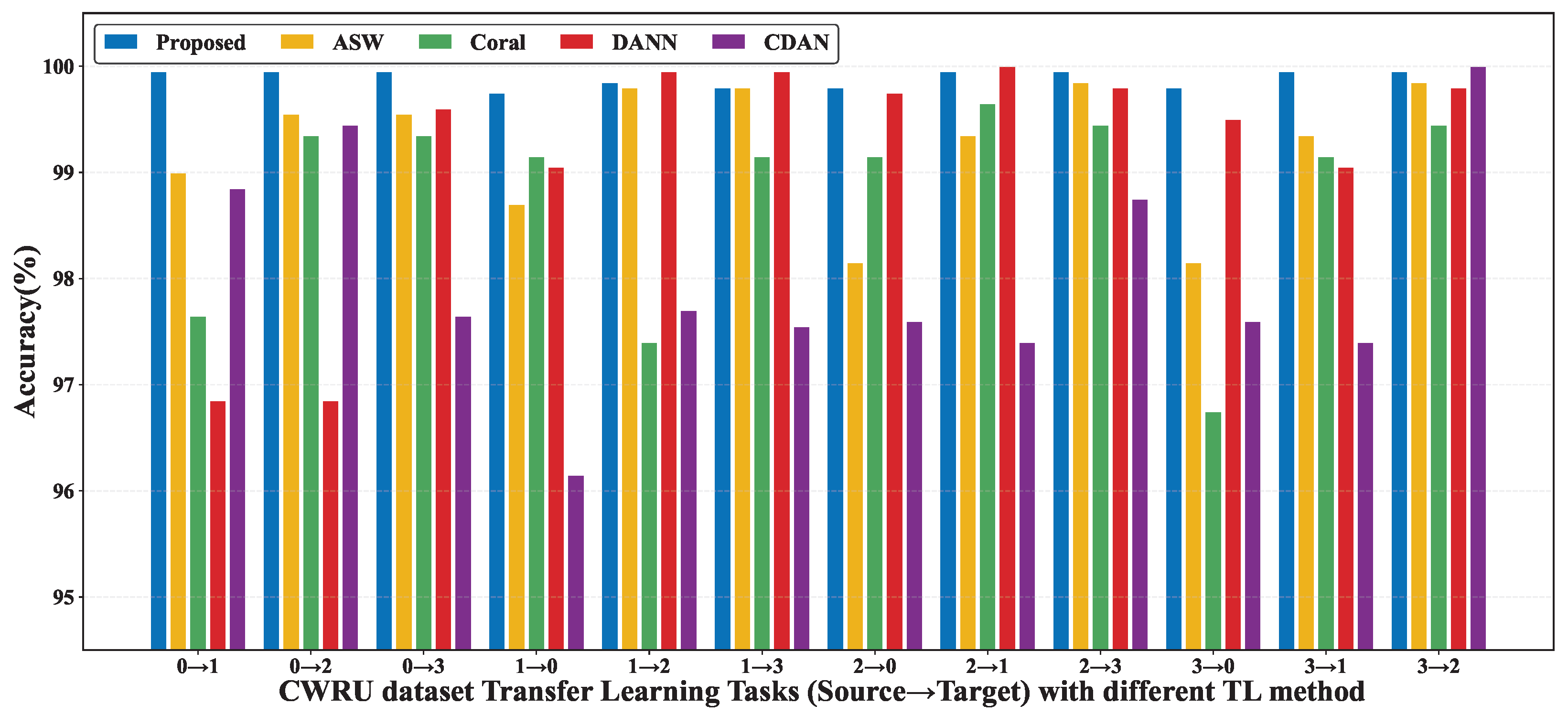
Figure 4 presents a comparative analysis of the proposed TL method against established TL (e.g., ASW, Coral, DANN, and CDAN) approaches. The proposed method demonstrated superior performance, efficiently capturing fault feature information and maintaining diagnostic accuracy even under significant speed fluctuations.

The proposed method consistently maintained high accuracy (99.95% and 99.75%), even under substantial variations in rotational speed (e.g., Task 0-3, Task 3-0), outperforming other TL approaches. While the ASW and CORAL methods effectively transfered pre-trained knowledge, their predictive accuracy (99.5% and 99.6%) was marginally inferior to our approach, despite their commendable performance on transfer learning tasks. Although CDAN and DANN demonstrated superior performance on specific tasks (99.99%), their overall performance was unstable, with significant performance degradation on the 0-1 and 1-0 (96.85% and 96.1%) domain adaptation tasks compared to our method.

From an industrial applicability perspective, the method’s consistent high accuracy across speed domains and its label-efficient design (requiring only source-domain labels) address two major practical challenges: the expense of data annotation and the prevalence of variable operating conditions. These advantages, combined with computational efficiency, make the method particularly suitable for real-world deployment, where equipment often operates under non-stationary speeds.

To validate the generalization capability of the proposed method across different scenarios, we conducted transfer learning experiments on the JNU dataset under various tasks. Specifically, two transfer learning tasks were examined, gear and bearing, resulting in a total of four transfer scenarios. The experiments involved different operational conditions, including varying rotational speeds (20 kHz and 30 kHz) and different working voltages (0 V and 2 V). Each task represented a domain adaptation scenario, where the model was trained on data from a source domain and tested on data from a target domain. To ensure the reliability of the results, all experiments were repeated five times. The detailed results are presented in the accompanying Figure 5.

Figure 5 clearly demonstrates that the proposed method maintained a stable diagnostic accuracy (99.99% to 98.5%), even when the operating conditions differed substantially between source and target domains. Compared with the baseline approaches, ASW also achieved respectable accuracies (99.93% to 98.65%) across the various conditions, yet its performance remained slightly inferior to that of the proposed method. Although Coral, DANN, and CDAN attained high accuracies in the gear fault TL task, their diagnostic performance degraded markedly when applied to bearing fault diagnosis. (For Task 20-0 bearing, the accuracy was 69.7%, 71.95%, and 65.95%, respectively.) Consequently, the proposed approach exhibited superior generalization ability and robustness across heterogeneous operating conditions and fault types. To demonstrate that the proposed method remains effective even under significant variations in rotational speed, we conducted extensive experiments on the JNU dataset, which covers a speed range of 600 to 1000 rpm. These experiments encompass nine different operational conditions, including transitions from Task 0-1 and from Task 2-0. Each task represents a scenario under different domain conditions. The model was trained on a single scenario and tested across various target scenarios. To ensure the reliability of the experimental results, all tests were repeated five times, and the outcomes are shown in Figure 6.

Figure 6 visualizes the TL performance of the proposed method in six scenarios, each involving significant variations in rotational speed. Although certain comparative methods exhibited strengths in specific TL tasks (e.g., Coral and ASW), however, the proposed achieved significantly superior overall performance while demonstrating a more comprehensive capability for effective transfer learning across diverse domains.

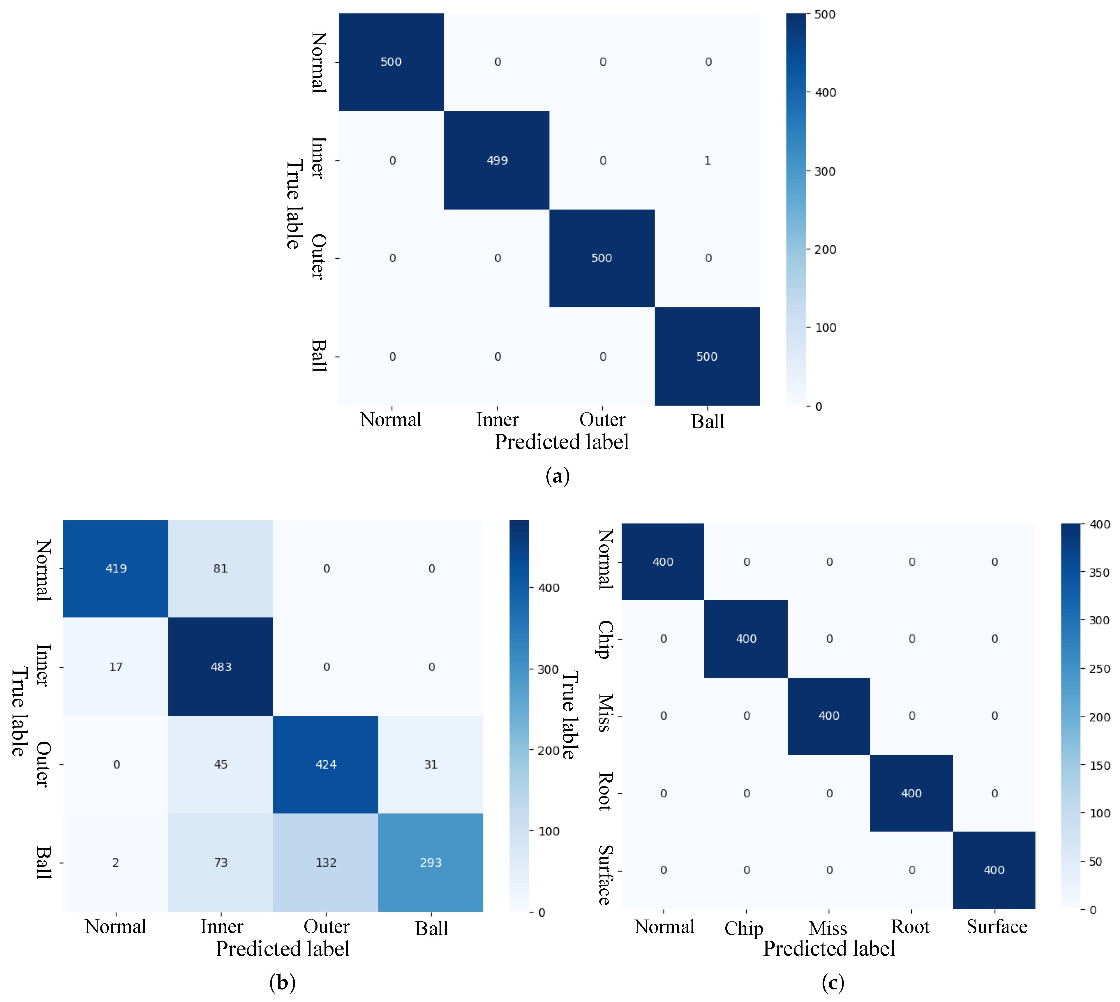
In Figure 7, we compared the confusion matrices of the proposed method for the 0-1 TL task across three different bearing datasets. To comparatively evaluate the efficacy of the proposed method, we validated its performance on diverse datasets, namely, CWRU, SEU, and JNU. The experimental results obtained for various approaches are presented in Figure 7. Figure 7a corresponds to the CWRU dataset. The diagonal elements show high counts, indicating strong classification ability for single-fault states in this well-known dataset. Figure 7b is from the SEU dataset. Here, the off-diagonal elements have non-zero values, meaning there are misclassifications, yet the diagonal still has relatively high values, reflecting the method’s performance with some interference in this dataset. Figure 7c pertains to the JNU dataset. The diagonal maintains considerable counts (e.g., 400 for normal, inner, outer; 390 for ball; 399 for comb), though there are minor misclassifications (like four misclassifications for ball and one for comb), showing the method’s adaptability across different data sources. Overall, Figure 7 presents the diagnostic accuracy of the proposed method across various datasets, thereby further validating its robust generalization capability across different data distributions.

To evaluate the performance of different methods in the target domain feature distribution, we compared the T-SNE visualizations of the proposed method with ASW and Coral, as illustrated in Figure 8. The analysis revealed that the proposed method significantly outperformed ASW and Coral in several aspects: (1) The distributions of different classes (Ball, Inner, Normal, Outer) were more concentrated and well separated, exhibiting high intra-class compactness and minimal inter-class overlap, whereas ASW and Coral showed significant class mixing. (2) The intra-class distributions of the proposed approach exhibited tighter clustering (e.g., Ball and Outer classes), whereas those generated by other methods displayed greater dispersion. (3) The proposed method exhibited superior control over the axis range, avoiding the influence of extreme outliers and indicating more stable feature extraction. Overall, the proposed method’s improved feature separation and aggregation capabilities, as demonstrated in Figure 8, suggest the potential for higher accuracy in classification or domain adaptation tasks.

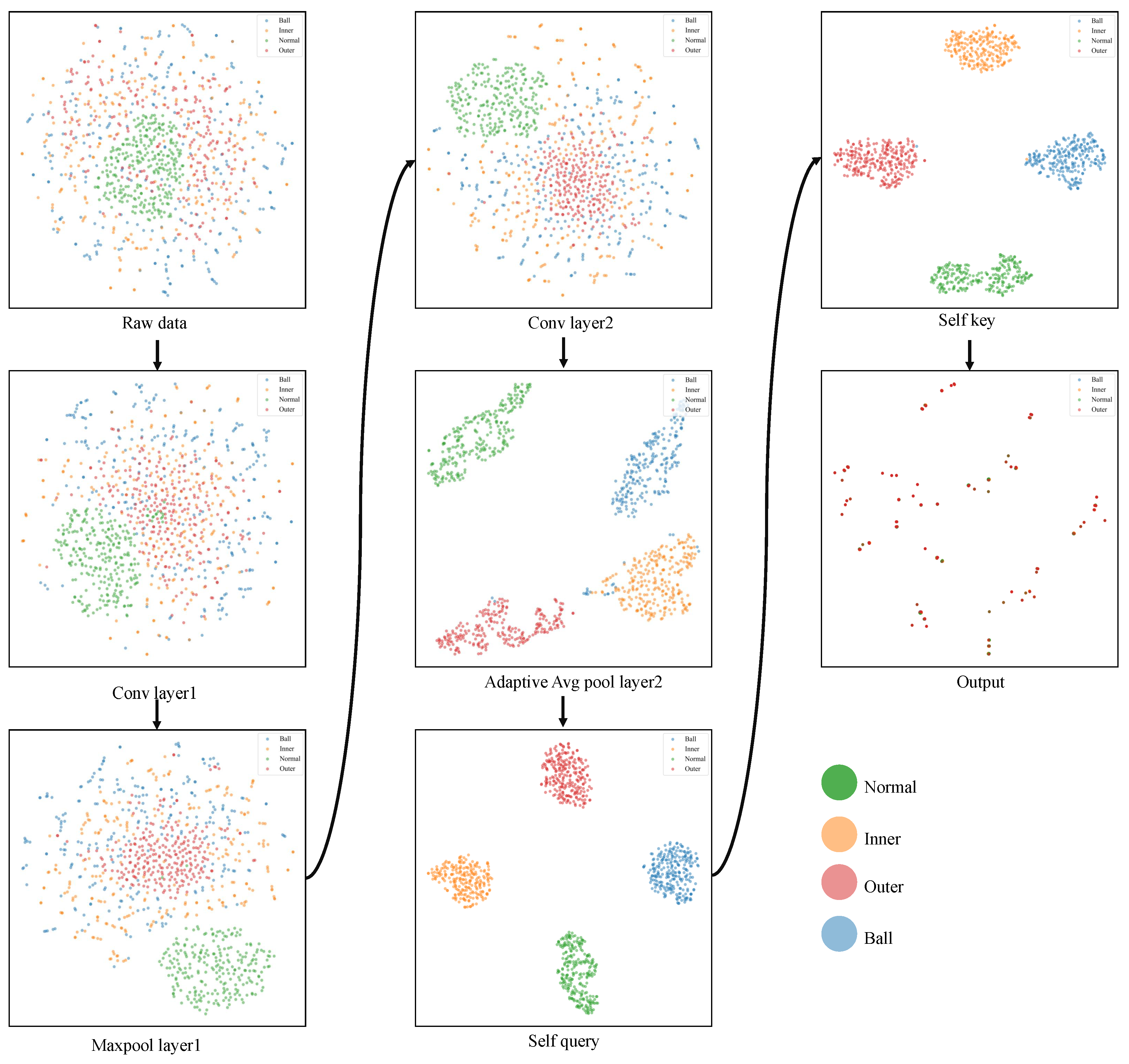
Figure 9 illustrates the architecture of the proposed CNN–Attention model for fault diagnosis, depicting the pipeline from raw data input to final classification output. The process begins with raw vibration signals, which are processed through Conv layer1 for initial feature extraction, followed by MaxPool1d to reduce dimensionality. The features then pass through another Conv layer2 and an Adaptive Average Pooling layer to generate a compact feature vector. The self-attention mechanism is applied next, where the feature vector is transformed into Query and Key matrices to compute attention weights, dynamically highlighting discriminative fault features. Finally, the weighted features are fed into a fully connected layer to produce the classification output, which includes four categories: Normal, Inner race fault, Outer race fault, and Ball fault. This visualization underscores the proposed model’s lightweight design and its ability to integrate local feature extraction with global dependency modeling, enabling robust fault diagnosis under variable operational conditions.

4.4. Comparison of Training Efficiency of Different Methods

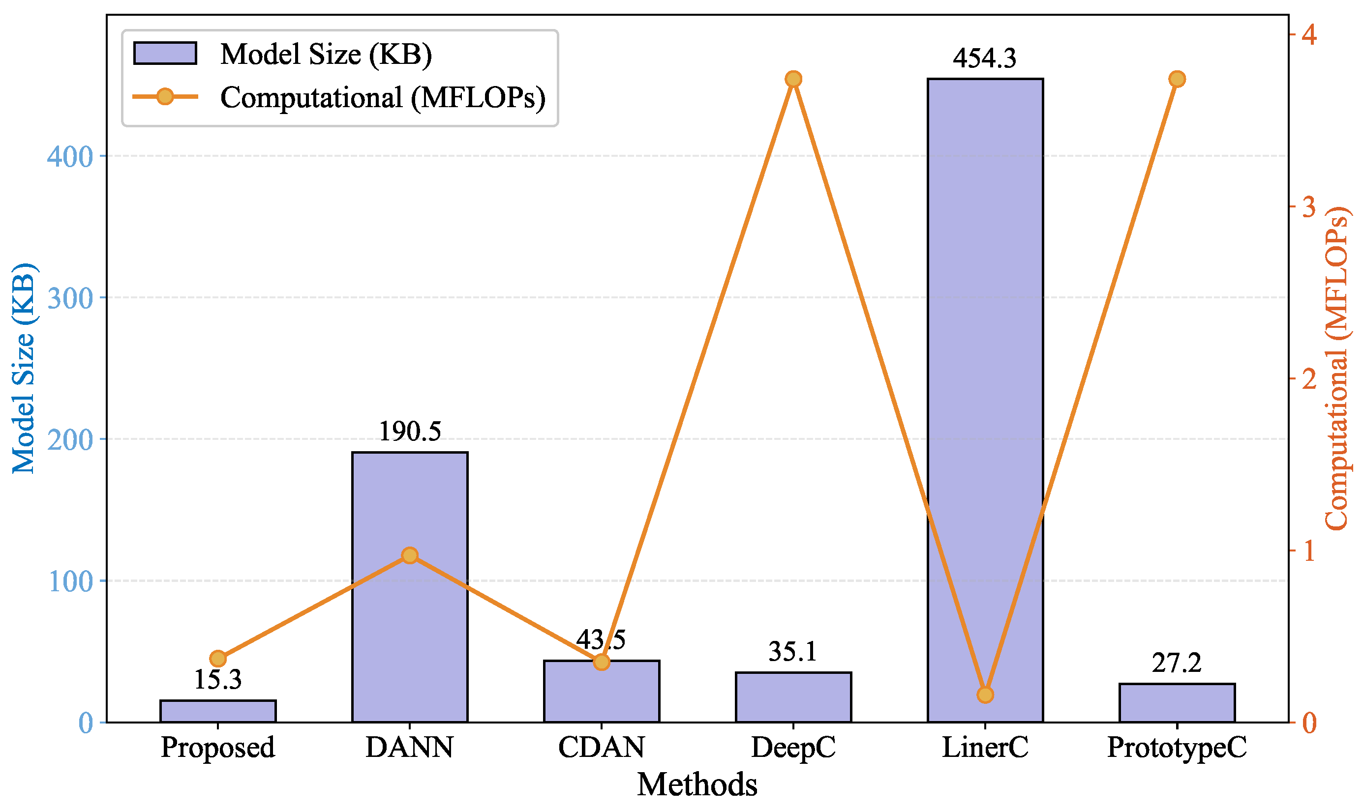
To evaluate the efficiency of the proposed TL method for bearing fault diagnosis under variable speed conditions, we conducted experiments with TL Task (0→1) on the CWRU dataset, examining three key performance aspects: model complexity, computational efficiency, and GPU utilization. The experiments compared our method against five approaches (DANN, DCAN, DeepC, LinearC, and PrototypeC) across 150 training epochs, with all tests conducted under identical hardware conditions to ensure fair comparison. As shown in Figure 10, the proposed method demonstrated consistent advantages across all evaluation metrics, establishing its superiority for industrial applications.

Model complexity metrics provide a direct measure of a method’s deployability. Our model achieved exceptional compactness, with a size of only 15.3 KB. Compared to LinearC (453 KB) and DANN (193 KB), this represents a size reduction of 96.63% and 92.06%, respectively, thereby significantly enhancing deployment feasibility while maintaining performance. Notably, while CDAN (43.5 KB), DeepC (35.1 KB), and ProtoC (27.2 KB) are also lightweight models, the proposed method exhibited no degradation in accuracy; indeed, it consistently outperformed these alternative lightweight architectures. Although Liner (0.19 MFLOPs) demonstrated lower computational requirements, the proposed method offers a substantial advantage in terms of model size, without compromising diagnostic accuracy. Moreover, when compared with other TL approaches, our method still achieved a substantially high diagnostic accuracy. This careful balance between complexity and performance is particularly valuable for edge deployment scenarios, where both memory footprint and computational budget are constrained.

As shown in Figure 11, computational efficiency tests demonstrate that the proposed method achieved its superior accuracy without excessive time cost, requiring 38.9 s of cumulative training time versus PrototypeC’s 42.7 s—a 9.1% reduction. This efficiency gain becomes more pronounced when considering the per-epoch time analysis, where our method maintained stable 0.25–2.7 s/epoch durations, while Coral showed greater variability (0.4–0.23 s). The time advantage is especially notable given that DANN and CDAN, while being the fastest (0.17–0.15 and 0.21–0.18 s/epoch), suffered from significantly lower accuracy (97.85% and 98.9%). This balance between speed and accuracy makes our method particularly suitable for real-time monitoring systems where both factors are critical.

Resource utilization analysis presents an interesting finding—the proposed method maintained moderate GPU usage (32.7% average) compared to PrototypeC’s higher consumption (31.62%) and LinearC’s peak usage (33.99%). This efficient resource management was achieved while delivering superior accuracy, contradicting the common assumption that higher performance necessitates greater resource expenditure. The GPU usage patterns also reveal our method’s better hardware adaptation, showing smoother utilization curves compared to the erratic fluctuations observed in Deepc (33.8% ± 2.5) and PrototypeC (31.62% ± 3.1). This stability suggests more consistent memory access patterns and better parallelization in our architecture. Looking at other approaches, DANN and CDAN demonstrate distinct GPU utilization patterns across training epochs. DANN’s GPU usage tended to fluctuate within a certain range (24–32%), reflecting its dynamic adaptation during training, while CDAN showed a relatively stable but moderately lower level (27–24%) compared to the proposed method, which could be due to its constraints in handling the complex data representations for robust feature extraction. ASW (34.12% ± 2.14) and Coral (29.71% ± 1.96), meanwhile, showed varying utilization trends, with occasional spikes that suggest periods of intensive computation during specific training phases but also periods of low activity, hinting at task-specific resource demands and potential bottlenecks.

The superior performance of the proposed method can be attributed to the effectiveness of the scaled dot-product attention mechanism. Unlike SE or CBAM, which rely on channel or spatial attention separately, our approach jointly models feature interactions across both dimensions. This is evident in the high accuracy (99.95%) achieved even under significant speed variations (e.g., Task 0-3), where SE/CBAM-based methods typically suffered from performance degradation due to their limited ability to capture global fault characteristics. Furthermore, the computational efficiency of our attention mechanism (as shown in Figure 10 and Figure 11) ensures real-time applicability, making it more suitable for industrial deployments compared to parameter-heavy alternatives.

The comprehensive evaluation reveals that the proposed method successfully addresses the key challenges in industrial fault diagnosis: achieving high accuracy across variable speeds (demonstrated by 99.99% final accuracy), maintaining computational efficiency (14.9% faster than PrototypeC), and enabling practical deployment (15.3 KB model size). These advantages stem from two key architectural innovations: the CNN and self-attention design that captures both local and global vibration patterns efficiently and the adaptive feature extraction strategy that reduces redundant computations. The method’s consistent performance across all metrics suggests it effectively avoids the common trade-off between accuracy and efficiency that plagues many deep learning approaches. From an industrial implementation perspective, the 15.3 KB model size makes the method deployable on resource-constrained edge devices, while the 0.37 MFLOPs computational requirement allows for real-time execution on modest hardware. These practical advantages, combined with the proven accuracy across variable speeds, position our method as a strong candidate for next-generation condition monitoring systems.

Compared to simulation-driven and zero-fault-shot methods, our approach demonstrates superior adaptability to variable speeds and loads without requiring synthetic data or fault templates. For example, while simulation-driven methods may struggle with domain shifts caused by unmodeled operational noise [57,58], our attention mechanism dynamically focuses on discriminative features, achieving 99.95% accuracy on the CWRU dataset. Similarly, zero-fault-shot methods often require auxiliary fault descriptions [59], whereas our method operates purely on vibration signals, making it more practical for industrial deployment.

5. Conclusions

Unlike simulation-driven or zero-fault-shot approaches, our method achieves high diagnostic accuracy without synthetic data or fault templates, relying instead on transfer learning and attention mechanisms for dynamic adaptation. This makes it particularly suitable for industrial applications where operational conditions are variable and labeled data is scarce.

This paper has presented a lightweight TL framework combining CNN and self-attention mechanisms for bearing fault diagnosis under variable speed conditions, specifically addressing the challenging scenario of unlabeled target domain data. The proposed architecture demonstrates three key advantages over conventional methods: (1) effective cross-domain knowledge transfer through strategic layer freezing, (2) robust feature learning via hybrid CNN–attention mechanisms, and (3) practical deployability with minimal computational overhead. Our experimental validation on the CWRU, SEU, and JNU datasets yielded several significant findings. First, the model achieved consistent accuracy between 99.95% and 98.85% across twelve transfer tasks (1730–1797 rpm) of CWRU, outperforming comparable methods by an average of 4.3% in cross-speed scenarios. Second, the two-phase training strategy—featuring frozen feature extractor during source training and frozen classifier during target adaptation—proved particularly effective for unlabeled target domains, reducing the need for annotated data while maintaining diagnostic reliability. Third, the compact 15.9 KB model size with 0.37 MFLOPs computational requirement confirms the solution’s suitability for edge deployment in industrial settings.

Future work will focus on extending this framework to more complex operational variations, including simultaneous changes in speed and load conditions. Additional research directions include investigating few-shot learning versions of the architecture for faster adaptation and exploring explainability techniques to enhance trust in the attention-based decisions. The current implementation already provides a practical solution for industries seeking to implement condition-based maintenance systems with limited labeled data, particularly in scenarios involving variable operational speeds.

References

1. Converso, G.; Gallo, M.; Murino, T.; Vespoli, S. Predicting Failure Probability in Industry 4.0 Production Systems: A Workload-Based Prognostic Model for Maintenance Planning. Appl. Sci. 2023, 13, 1938. [Google Scholar] [CrossRef]
2. Fu, C.; Sinou, J.J.; Zhu, W.; Lu, K.; Yang, Y. A state-of-the-art review on uncertainty analysis of rotor systems. Mech. Syst. Signal Process. 2023, 183, 109619. [Google Scholar] [CrossRef]
3. Yang, X.; Zhang, L.; Shu, L.; Jing, X.; Zhang, Z. SILF Dataset: Fault Dataset for Solar Insecticidal Lamp Internet of Things Node. Sensors 2025, 25, 2808. [Google Scholar] [CrossRef]
4. Badihi, H.; Zhang, Y.; Jiang, B.; Pillay, P.; Rakheja, S. A Comprehensive Review on Signal-Based and Model-Based Condition Monitoring of Wind Turbines: Fault Diagnosis and Lifetime Prognosis. Proc. IEEE 2022, 110, 754–806. [Google Scholar] [CrossRef]
5. Aqamohammadi, A.R.; Niknam, T.; Shojaeiyan, S.; Siano, P.; Dehghani, M. Deep Neural Network with Hilbert–Huang Transform for Smart Fault Detection in Microgrid. Electronics 2023, 12, 499. [Google Scholar] [CrossRef]
6. Hu, C.; Wu, J.; Sun, C.; Chen, X.; Nandi, A.K.; Yan, R. Unified Flowing Normality Learning for Rotating Machinery Anomaly Detection in Continuous Time-Varying Conditions. IEEE Trans. Cybern. 2025, 55, 221–233. [Google Scholar] [CrossRef] [PubMed]
7. Jeong, E.; Yang, J.H.; Lim, S.C. Deep Neural Network for Valve Fault Diagnosis Integrating Multivariate Time-Series Sensor Data. Actuators 2025, 14, 70. [Google Scholar] [CrossRef]
8. Jung, H.; Choi, S.; Lee, B. Rotor Fault Diagnosis Method Using CNN-Based Transfer Learning with 2D Sound Spectrogram Analysis. Electronics 2023, 12, 480. [Google Scholar] [CrossRef]
9. Huang, D.; Zhang, W.A.; Guo, F.; Liu, W.; Shi, X. Wavelet Packet Decomposition-Based Multiscale CNN for Fault Diagnosis of Wind Turbine Gearbox. IEEE Trans. Cybern. 2023, 53, 443–453. [Google Scholar] [CrossRef]
10. Gawde, S.; Patil, S.; Kumar, S.; Kamat, P.; Kotecha, K.; Abraham, A. Multi-fault diagnosis of Industrial Rotating Machines using Data-driven approach: A review of two decades of research. Eng. Appl. Artif. Intell. 2023, 123, 106139. [Google Scholar] [CrossRef]
11. Nie, L.; Ren, Y.; Wu, R.; Tan, M. Sensor Fault Diagnosis, Isolation, and Accommodation for Heating, Ventilating, and Air Conditioning Systems Based on Soft Sensor. Actuators 2023, 12, 389. [Google Scholar] [CrossRef]
12. Guo, C.; Sun, Y.; Yu, R.; Ren, X. Deep Causal Disentanglement Network with Domain Generalization for Cross-Machine Bearing Fault Diagnosis. IEEE Trans. Instrum. Meas. 2025, 74, 3512616. [Google Scholar] [CrossRef]
13. Younesi, A.; Ansari, M.; Fazli, M.; Ejlali, A.; Shafique, M.; Henkel, J. A Comprehensive Survey of Convolutions in Deep Learning: Applications, Challenges, and Future Trends. IEEE Access 2024, 12, 41180–41218. [Google Scholar] [CrossRef]
14. LI, G.; GENG, H.; XIE, F.; XU, C.; XU, Z. Ensemble Deep Transfer Learning Method for Fault Diagnosis of Waterjet Pump Under Variable Working Conditions. Ship Boat 2025, 36, 103. [Google Scholar] [CrossRef]
15. Sun, B.; Saenko, K. Deep coral: Correlation alignment for deep domain adaptation. In Proceedings of the Computer Vision–ECCV 2016 Workshops, Amsterdam, The Netherlands, 8–10, 15–16 October 2016; Proceedings, Part III 14. Springer: Cham, Switzerland, 2016; pp. 443–450. [Google Scholar] [CrossRef]
16. Borgwardt, K.M.; Gretton, A.; Rasch, M.J.; Kriegel, H.P.; Schölkopf, B.; Smola, A.J. Integrating structured biological data by Kernel Maximum Mean Discrepancy. Bioinformatics 2006, 22, e49–e57. [Google Scholar] [CrossRef]
17. Zhang, X.; Zhang, X.; Liang, W.; He, F. Research on rolling bearing fault diagnosis based on parallel depthwise separable ResNet neural network with attention mechanism. Expert Syst. Appl. 2025, 286, 128105. [Google Scholar] [CrossRef]
18. Cui, J.; Li, Y.; Zhang, Q.; Wang, Z.; Du, W.; Wang, J. Multi-layer adaptive convolutional neural network unsupervised domain adaptive bearing fault diagnosis method. Meas. Sci. Technol. 2022, 33, 085009. [Google Scholar] [CrossRef]
19. An, Y.; Zhang, K.; Chai, Y.; Zhu, Z.; Liu, Q. Gaussian Mixture Variational-Based Transformer Domain Adaptation Fault Diagnosis Method and Its Application in Bearing Fault Diagnosis. IEEE Trans. Ind. Informatics 2024, 20, 615–625. [Google Scholar] [CrossRef]
20. Ding, P.; Jia, M.; Ding, Y.; Zhao, X. Statistical Alignment-Based Metagated Recurrent Unit for Cross-Domain Machinery Degradation Trend Prognostics Using Limited Data. IEEE Trans. Instrum. Meas. 2021, 70, 3511212. [Google Scholar] [CrossRef]
21. Chen, X.; Shao, H.; Xiao, Y.; Yan, S.; Cai, B.; Liu, B. Collaborative fault diagnosis of rotating machinery via dual adversarial guided unsupervised multi-domain adaptation network. Mech. Syst. Signal Process. 2023, 198, 110427. [Google Scholar] [CrossRef]
22. Kim, T.; Chai, J. Fault Diagnosis of Bearings with the Common-Domain Data. IEEE Access 2022, 10, 45457–45470. [Google Scholar] [CrossRef]
23. Xiao, H.; Dong, L.; Wang, W.; Ogai, H. Distribution Sub-Domain Adaptation Deep Transfer Learning Method for Bridge Structure Damage Diagnosis Using Unlabeled Data. IEEE Sensors J. 2022, 22, 15258–15272. [Google Scholar] [CrossRef]
24. Zhang, J.; Pei, G.; Zhu, X.; Gou, X.; Deng, L.; Gao, L.; Liu, Z.; Ni, Q.; Lin, J. Diesel engine fault diagnosis for multiple industrial scenarios based on transfer learning. Measurement 2024, 228, 114338. [Google Scholar] [CrossRef]
25. Zhang, D.; Zhou, T. Deep Convolutional Neural Network Using Transfer Learning for Fault Diagnosis. IEEE Access 2021, 9, 43889–43897. [Google Scholar] [CrossRef]
26. Farag, M.M. Towards a Standard Benchmarking Framework for Domain Adaptation in Intelligent Fault Diagnosis. IEEE Access 2025, 13, 24426–24453. [Google Scholar] [CrossRef]
27. Tang, S.; Ma, J.; Yan, Z.; Zhu, Y.; Khoo, B.C. Deep transfer learning strategy in intelligent fault diagnosis of rotating machinery. Eng. Appl. Artif. Intell. 2024, 134, 108678. [Google Scholar] [CrossRef]
28. Ibrahim, A.; Anayi, F.; Packianather, M. New Transfer Learning Approach Based on a CNN for Fault Diagnosis. Eng. Proc. 2022, 24, 16. [Google Scholar] [CrossRef]
29. Zhu, C.; Lin, W.; Zhang, H.; Cao, Y.; Fan, Q.; Zhang, H. Research on a Bearing Fault Diagnosis Method Based on an Improved Wasserstein Generative Adversarial Network. Machines 2024, 12, 587. [Google Scholar] [CrossRef]
30. Shakiba, F.M.; Shojaee, M.; Azizi, S.M.; Zhou, M. Transfer Learning for Fault Diagnosis of Transmission Lines. arXiv 2022, arXiv:2201.08018. [Google Scholar] [CrossRef]
31. Wang, Q.; Michau, G.; Fink, O. Domain Adaptive Transfer Learning for Fault Diagnosis. In Proceedings of the 2019 Prognostics and System Health Management Conference (PHM-Paris), Paris, France, 2–5 May 2019; pp. 279–285. [Google Scholar] [CrossRef]
32. Liu, Y.; Zhang, X.; Wang, Y.; Zhou, Y.; Jia, L. Machinery Fault Diagnosis for Imbalanced Samples via Coupled Generative Adversarial Networks. In Proceedings of the 2024 43rd Chinese Control Conference (CCC), Kunming, China, 28–31 July 2024; pp. 8951–8956. [Google Scholar] [CrossRef]
33. Zhao, B.; Cheng, C.; Peng, Z.; He, Q.; Meng, G. Hybrid Pre-Training Strategy for Deep Denoising Neural Networks and Its Application in Machine Fault Diagnosis. IEEE Trans. Instrum. Meas. 2021, 70, 3526811. [Google Scholar] [CrossRef]
34. Wu, M.; Zhang, J.; Xu, P.; Liang, Y.; Dai, Y.; Gao, T.; Bai, Y. Bearing Fault Diagnosis for Cross-Condition Scenarios Under Data Scarcity Based on Transformer Transfer Learning Network. Electronics 2025, 14, 515. [Google Scholar] [CrossRef]
35. Asutkar, S.; Chalke, C.; Shivgan, K.; Tallur, S. TinyML-enabled edge implementation of transfer learning framework for domain generalization in machine fault diagnosis. Expert Syst. Appl. 2023, 213, 119016. [Google Scholar] [CrossRef]
36. Yan, Z.; Zhang, Z.; Liu, S. Improving Performance of Seismic Fault Detection by Fine-Tuning the Convolutional Neural Network Pre-Trained with Synthetic Samples. Energies 2021, 14, 3650. [Google Scholar] [CrossRef]
37. Di Maggio, L.G. Intelligent Fault Diagnosis of Industrial Bearings Using Transfer Learning and CNNs Pre-Trained for Audio Classification. Sensors 2023, 23, 211. [Google Scholar] [CrossRef]
38. Chakraborty, S.; Uzkent, B.; Ayush, K.; Tanmay, K.; Sheehan, E.; Ermon, S. Efficient Conditional Pre-training for Transfer Learning. In Proceedings of the 2022 IEEE/CVF Conference on Computer Vision and Pattern Recognition Workshops (CVPRW), New Orleans, LA, USA, 19–20 June 2022; pp. 4240–4249. [Google Scholar] [CrossRef]
39. Udmale, S.S.; Singh, S.K.; Singh, R.; Sangaiah, A.K. Multi-Fault Bearing Classification Using Sensors and ConvNet-Based Transfer Learning Approach. IEEE Sensors J. 2020, 20, 1433–1444. [Google Scholar] [CrossRef]
40. Pei, X.; Zheng, X.; Wu, J. Rotating Machinery Fault Diagnosis Through a Transformer Convolution Network Subjected to Transfer Learning. IEEE Trans. Instrum. Meas. 2021, 70, 2515611. [Google Scholar] [CrossRef]
41. Dai, X.; Gao, Z. From Model, Signal to Knowledge: A Data-Driven Perspective of Fault Detection and Diagnosis. IEEE Trans. Ind. Inform. 2013, 9, 2226–2238. [Google Scholar] [CrossRef]
42. Ding, Q.; Zheng, F.; Liu, L.; Li, P.; Shen, M. Swift Transfer of Lactating Piglet Detection Model Using Semi-Automatic Annotation Under an Unfamiliar Pig Farming Environment. Agriculture 2025, 15, 696. [Google Scholar] [CrossRef]
43. Dong, F.; Yang, J.; Cai, Y.; Xie, L. Transfer learning-based fault diagnosis method for marine turbochargers. Actuators 2023, 12, 146. [Google Scholar] [CrossRef]
44. Lin, Y.C.; Huang, Y.C. Streamlined Deep Learning Models for Move Prediction in Go-Game. Electronics 2024, 13, 93. [Google Scholar] [CrossRef]
45. Nguyen, C.T.; Van Huynh, N.; Chu, N.H.; Saputra, Y.M.; Hoang, D.T.; Nguyen, D.N.; Pham, Q.V.; Niyato, D.; Dutkiewicz, E.; Hwang, W.J. Transfer Learning for Wireless Networks: A Comprehensive Survey. Proc. IEEE 2022, 110, 1073–1115. [Google Scholar] [CrossRef]
46. Hao, S.; Li, J.; Ma, X.; Sun, S.; Tian, Z.; Li, T.; Hou, Y. A Photovoltaic Hot-Spot Fault Detection Network for Aerial Images Based on Progressive Transfer Learning and Multiscale Feature Fusion. IEEE Trans. Geosci. Remote Sens. 2024, 62, 4709713. [Google Scholar] [CrossRef]
47. Zeng, Y.; Sun, B.; Xu, R.; Qi, G.; Wang, F.; Zhang, Z.; Wu, K.; Wu, D. Multirepresentation Dynamic Adaptive Network for Cross-Domain Rolling Bearing Fault Diagnosis in Complex Scenarios. IEEE Trans. Instrum. Meas. 2025, 74, 3522716. [Google Scholar] [CrossRef]
48. Lv, K.; Yang, Y.; Liu, T.; Gao, Q.; Guo, Q.; Qiu, X. Full parameter fine-tuning for large language models with limited resources. arXiv 2023, arXiv:2306.09782. [Google Scholar] [CrossRef]
49. Zhao, Z.; Zhang, Q.; Yu, X.; Sun, C.; Wang, S.; Yan, R.; Chen, X. Applications of Unsupervised Deep Transfer Learning to Intelligent Fault Diagnosis: A Survey and Comparative Study. IEEE Trans. Instrum. Meas. 2021, 70, 3525828. [Google Scholar] [CrossRef]
50. Neupane, D.; Seok, J. Bearing Fault Detection and Diagnosis Using Case Western Reserve University Dataset with Deep Learning Approaches: A Review. IEEE Access 2020, 8, 93155–93178. [Google Scholar] [CrossRef]
51. AlShalalfeh, A.; Shalalfeh, L. Bearing Fault Diagnosis Approach Under Data Quality Issues. Appl. Sci. 2021, 11, 3289. [Google Scholar] [CrossRef]
52. Li, C.; Mo, L.; Yan, R. Fault Diagnosis of Rolling Bearing Based on WHVG and GCN. IEEE Trans. Instrum. Meas. 2021, 70, 3519811. [Google Scholar] [CrossRef]
53. Qian, C.; Jiang, Q.; Shen, Y.; Huo, C.; Zhang, Q. An intelligent fault diagnosis method for rolling bearings based on feature transfer with improved DenseNet and joint distribution adaptation. Meas. Sci. Technol. 2021, 33, 025101. [Google Scholar] [CrossRef]
54. Fanai, H.; Abbasimehr, H. A novel combined approach based on deep Autoencoder and deep classifiers for credit card fraud detection. Expert Syst. Appl. 2023, 217, 119562. [Google Scholar] [CrossRef]
55. Rymarczyk, D.; Struski, Ł.; Górszczak, M.; Lewandowska, K.; Tabor, J.; Zieliński, B. Interpretable Image Classification with Differentiable Prototypes Assignment. In Proceedings of the Computer Vision—ECCV 2022, Tel Aviv, Israel, 23–27 October 2022; Springer: Cham, Switzerland, 2022; pp. 351–368. [Google Scholar] [CrossRef]
56. Evron, I.; Moroshko, E.; Buzaglo, G.; Khriesh, M.; Marjieh, B.; Srebro, N.; Soudry, D. Continual Learning in Linear Classification on Separable Data. In Proceedings of the 40th International Conference on Machine Learning, Honolulu, HI, USA, 23–29 July 2023; Krause, A., Brunskill, E., Cho, K., Engelhardt, B., Sabato, S., Scarlett, J., Eds.; PMLR: Cambridge, MA, USA, 2023; Volume 202, Proceedings of Machine Learning Research. pp. 9440–9484. [Google Scholar]
57. Liu, C.; Gryllias, K. Simulation-Driven Domain Adaptation for Rolling Element Bearing Fault Diagnosis. IEEE Trans. Ind. Inform. 2022, 18, 5760–5770. [Google Scholar] [CrossRef]
58. Jiao, X.; Zhang, J.; Cao, J. A Bearing Fault Diagnosis Method Based on Dual-Stream Hybrid-Domain Adaptation. Sensors 2025, 25, 3686. [Google Scholar] [CrossRef]
59. Jeong, H.; Kim, S.; Seo, D.; Kwon, J. Source-Free Domain Adaptation Framework for Rotary Machine Fault Diagnosis. Sensors 2025, 25, 4383. [Google Scholar] [CrossRef]
Figure 1. Two-phase TL framework for bearing fault diagnosis under variable speeds. The upper section illustrates source-domain training with frozen feature extractor layers, where labeled source data are processed through CNN layers to train the attention classifier. The lower section shows target-domain adaptation with frozen classifier layers, where unlabeled target data adapt the feature extractor while maintaining the pre-trained classifier.
Actuators 14 00415 g001
Figure 2. Cross-domain bearing fault diagnosis accuracy comparison, where bar charts with blue, yellow, red, and purple represent the proposed method, DeepC, PrototypeC, and LinearC methods, respectively.
Actuators 14 00415 g002
Figure 3. Comparison of confusion matrices for different methods: (a) proposed method, (b) DeepC, (c) ProtoC, (d) LinerC (Class0 is Normal label, Class1 is Inner fault label, Class2 is Outer fault label, Class3 is Ball fault label).
Actuators 14 00415 g003
Figure 4. CWRU cross-domain bearing fault diagnosis accuracy comparison, where bar charts with blue, yellow, green, red, and purple represent the proposed method, ASW, Coral, DANN, and CDAN methods, respectively.
Actuators 14 00415 g004
Figure 5. SEU cross-domain bearing fault diagnosis accuracy comparison, where bar charts with blue, yellow, green, red, and purple represent the proposed method, ASW, Coral, DANN, and CDAN methods, respectively.
Actuators 14 00415 g005
Figure 6. JNU cross-domain bearing fault diagnosis accuracy comparison, where bar charts with blue, yellow, green, red, and purple represent the proposed method, ASW, Coral, DANN, and CDAN methods, respectively.
Actuators 14 00415 g006
Figure 7. Comparison of confusion matrices for different datasets: (a) CWRU 0-1 TL task, (b) JNU 0-1 TL task, (c) SEU 0-1 TL task.
Actuators 14 00415 g007
Figure 8. T-SNE of different methods in CWRU Task 0-1: (a) Proposed. (b) ASW. (c) Coral. The green, yellow, blue, and red dots in the figure correspond to the data of health, inner, ball, and outer, respectively.
Actuators 14 00415 g008
Figure 9. The visualization illustrates the architecture of the proposed method, with each class rendered using specific color-coding to represent distinct classes: Normal (green), Inner (yellow), Outer (red), and Ball (blue).
Actuators 14 00415 g009
Figure 10. Model size and computational of different method.
Actuators 14 00415 g010
Figure 11. Training efficiency of different methods: (a) Memory usage comparison. (b) Computational efficiency comparison.
Actuators 14 00415 g011