Fault Diagnosis Method of Micro-Motor Based on Jump Plus AM-FM Mode Decomposition and Symmetrized Dot Pattern

Abstract

Micro-motors are essential for power drive systems, and efficient fault diagnosis is crucial to reduce safety risks and economic losses caused by failures. However, the fault signals from micro-motors typically exhibit weak and unclear characteristics. To address this challenge, this paper proposes a novel fault diagnosis method that integrates jump plus AM-FM mode decomposition (JMD), symmetrized dot pattern (SDP) visualization, and an improved convolutional neural network (ICNN). Firstly, we employed the jump plus AM-FM mode decomposition technique to decompose the mixed fault signals, addressing the problem of mode mixing in traditional decomposition methods. Then, the intrinsic mode functions (IMFs) decomposed by JMD serve as the multi-channel inputs for symmetrized dot pattern, constructing a two-dimensional polar coordinate petal image. This process achieves both signal reconstruction and visual enhancement of fault features simultaneously. Finally, this paper designed an ICNN method with LeakyReLU activation function to address the vanishing gradient problem and enhance classification accuracy and training efficiency for fault diagnosis. Experimental results indicate that the proposed JMD-SDP-ICNN method outperforms traditional methods with a significantly superior fault classification accuracy of up to 99.2381%. It can offer a potential solution for the monitoring of electromechanical structures under complex conditions.

1. Introduction

Micro-motors are essential power-drive components in industrial production. Their precise internal design enables high output efficiency with minimal input power [1]. They are widely used in various fields, such as military, medical, and aircraft, where high reliability standards are essential [2]. However, challenges such as inconsistent production quality, component wear, and temperature fluctuations can lead to various motor faults, including commutator wear [3], shaft bending [4], housing deformation [5], etc. These faults can threaten safety and lead to economic losses or personal injuries. Therefore, an enhanced fault diagnosis technology is crucial for accurately assessing the health of micro-motors, identifying potential issues, and ensuring reliable performance.

Recently, researchers have conducted comprehensive analyses of various fault diagnosis techniques using intelligent sensing signals, including vibration signals [6], current signals [7], and temperature signals [8]. However, considering the characteristics of the small size and light weight of the micro-motor, the traditional contact signal measurement methods are no longer effective. Therefore, this paper proposes a non-contact sound measurement method for fault diagnosis. Moreover, the original signals obtained through this method are typically weak, so the subsequent signal processing and feature enhancement will be performed to achieve a good diagnosis effect.

Most real signals consist of various frequencies, amplitudes, and phases, which often capture environmental noise and electromagnetic interference. So, it is important to perform modal decomposition to extract signals that are closely related to the physical parameters of the motor. Techniques such as empirical mode decomposition (EMD) [9] and variational mode decomposition (VMD) [10] have proven effective in decomposing oscillation signals, but they can encounter mode aliasing issues during the process. In 2024, M. Nazari et al. [11] first introduced a new method called Jump plus AM-FM mode decomposition (JMD), which addresses the challenges of aliasing in non-stationary signals. This approach was initially developed for the analysis of Earth’s electric field signals, as well as electrocardiograms and electroencephalograms. The paper concludes that JMD can simultaneously and explicitly separate the jump component and the multi-scale oscillation component, thereby solving the problem that EMD and VMD mistakenly mix the jump component with the high-frequency oscillation when there are jumps. When a motor encounters faults such as bearing wear, impacts, or rotor imbalance, it produces some jump components superimposed on the original oscillation signals. As a result, the measured sound signal comprises both regular vibrations and sudden impacts. This characteristic matches well with the advantages of the JMD method. Thus, this paper will employ the JMD technique for the feature decomposition and extraction of sound signals produced by micro-motors.

Machine learning algorithms detect faults by analyzing feature information, with classification accuracy being greatly influenced by these features [12]. Thus, it is essential to investigate feature enhancement methods that can improve the accuracy of micro-motor fault classification. Compared with one-dimensional signals, two-dimensional images can provide more detailed and distinct features through techniques such as texture analysis and shape recognition [13]. The symmetrized dot pattern (SDP) method, initially introduced in [14], is a technique that transforms a time-domain signal into a symmetrical petal plot within a polar coordinate system. This method effectively captures waveform characteristics through the distinct shapes of the petals, offering a straightforward calculation process [15]. X. Zhu et al. [16] improved this method by using multiple sensor signals to increase fault recognition accuracy from 92% to 96.5%. Based on the above principles, we construct the IMFs as multi-channel parameters of SDP to integrate the intrinsic multi-scale information features of the signal and significantly enhance the discriminability of these features.

CNN is a classic type of neural network that can effectively analyze and recognize features in input images, demonstrating its superior abilities in image classification tasks [17]. However, in traditional CNNs, the ReLU activation function can lead to gradient vanishing because its gradient is zero for negative inputs. The ReLU function outputs zero if the input is less than zero. This can lead to permanent inactivation of some neurons during training, a so-called “neuron death” which hinders effective training of deep networks. LeakyReLU addresses this issue by introducing a non-zero negative slope, allowing gradients to flow more effectively and improving the stability of the training process [18]. Since image data may contain various features, including some negative feature vectors, using LeakyReLU instead of ReLU can capture these features more comprehensively. Therefore, we developed an improved CNN method (ICNN) using the LeakyReLU function to increase both training accuracy and efficiency.

In this study, we combined the strengths of JMD and SDP for feature extraction, proposed a novel ICNN method to improve learning and recognition efficiency, and developed a fault diagnosis method for rotating machinery. First, the preprocessed signals are decomposed using the JMD decomposition method. The IMFs are subsequently identified as the feature extraction objects based on the correlation coefficient–energy criterion. Following this, the extracted IMFs were transformed into SDP images. Finally, the resulting images from the JMD-SDP process served as the input for the micro-motor fault diagnosis model, in which the ICNN method was employed for learning. Compared with some traditional combinations such as STFT-CNN and VMD-SVM, the proposed method achieves superior diagnostic accuracy and robustness for weak and non-stationary fault signals. While STFT-CNN methods are limited by the time–frequency resolution trade-off [19], and SVM-based classifiers are less effective for complex or nonlinear feature spaces [20], our approach leverages adaptive mode decomposition and deep learning to deliver more reliable and interpretable results.

This paper is organized as follows: Section 2 discusses the principles of fault diagnosis using the JMD-SDP-ICNN method and then compares the accuracy of signal decomposition among JMD, EMD, and VMD. Section 3 offers a detailed description of the experimental platform and constructs the test set. In Section 4, the efficiency and accuracy of the fault method proposed in this paper are verified through a series of comparative tests. Finally, Section 5 summarizes the main conclusions of this study.

2. Basic Theory of JMD-SDP-ICNN

2.1. The Principle of Jump Plus AM-FM Mode Decomposition

Signals measured during the operation of an electric motor are often a combination of oscillations, jumps, and periodic signals. The JMD method effectively separates and divides the frequency domain of the oscillatory and jump components by solving a variational optimization problem. In this optimization objective, JMD imposes a minimizing bandwidth constraint on the oscillatory components, ensuring their spectral energy is concentrated, while applying a sparsity regularization on the derivative of the jump component, resulting in a discontinuous structure that captures abrupt changes. This dual constraint not only prevents traditional EMD or VMD methods from misclassifying jumps as high-frequency oscillations but also overcomes the limitation of conventional jump extraction approaches, which cannot further decompose multi-scale oscillations after removing jumps. Consequently, JMD enables accurate and distinct separation of oscillatory and jump components.

Initially, we assumed that the motor signal consists of three components: oscillatory components, jump components, and noise. From a mathematical perspective, the signal was assumed to be as follows [11]:

$$f\left(t\right)={\displaystyle \sum }_{k=1}^K{u}_k\left(t\right)+v\left(t\right)+n\left(t\right)$$

(1)

where $K$ denotes the number of oscillatory components in the input signal, $v\left(t\right)$ represents the jump component in the input data, and $n\left(t\right)$ is noise. The JMD computes $u_k\left(t\right)$ and $v\left(t\right)$ by processing the provided input signals. Next, to effectively separate the discontinuity component from the oscillatory components in the original signal, an optimal function must be constructed and solved as a minimization problem [21]. The JMD method mainly achieves signal decomposition through the following steps:

• To effectively extract the oscillatory components from the signal, the bandwidth of the oscillatory components must be minimized. The optimization equation that employs the VMD algorithm is as follows:

  $$J_1={\displaystyle \sum }_k{‖{\partial }_t\left[u_{k+}\left(t\right)e^{-j{\omega }_{k}t}\right]‖}_2^2$$

  (2)

  where ${\partial }_t$ denotes the partial derivative with respect to time, and ${\omega }_k$ is the center frequency associated with each mode. $u_{k+}(t)=u_k\left(t\right)+j\mathrm{H}{u}_k\left(t\right)= a_k\left(t\right)e^{j{\varphi }_k(t)}$ represents the analytic signal, and $\mathrm{H}$ refers to the Hilbert transform. ${‖·‖}_2^2$ estimates the bandwidth of the oscillatory mode of the signal.
• The extraction of the jump component from the signal is accomplished by applying a reparametrized and rescaled minimax concave penalty term [22]. By imposing constraints on the derivative of the jump component, this approach enhances the representation of discontinuities while effectively preserving the amplitude of the piecewise continuous signal component.

  $$J_2={{\displaystyle \int }}_0^{\infty }\varphi (\left|{\partial }_{\mathrm{t}}v(t)\right|;b)dt$$

  (3)

  where ${\partial }_t$ represents the first derivative of the jump term, and $\varphi (·;b):\left[0,+\infty \right]\to \left[0,1\right]$ is defined as a piecewise quadratic function as follows [23]:

  $$\varphi \left(x;b\right)=\left\{\begin{array}{c}-{\displaystyle \frac{b}{2}}{x}^2+\sqrt{2b}x x\in \left[0,\sqrt{2/b}\right)\\ 1 x\in \left[\sqrt{2/b},+\infty \right)\hfill \end{array}\right.$$

  (4)

  where the parameter $b$ alters the degree of nonconvexity. When $b\to 0$, the minimax concave penalty term is defined as $\varphi (·;b)=\left|x\right|$ and $b\to \infty$, whereas $\varphi (·;b)=\left|x\right|$ tends toward the $l_0$ pseudo-norm.
• To extract the jump and oscillation variables from $f\left(t\right)$, we combined $J_1$ from Equation (2) and $J_2$ from Equation (3), using the parameters $\alpha$ and $\beta$ to balance the two terms. Simultaneously, an auxiliary variable $x={\partial }_{t}v$ was introduced to address the issue of non-differentiability in the $\varphi (·;b)$ term. This approach allows the formulation of the problem using the following optimization equation:

  $$\begin{array}{l}(\left\{{u^{\ast }}_k\right\},\left\{{{\omega }^{\ast }}_k\right\},v^{\ast },x)\leftarrow \underset{\left\{u_k\right\},\left\{{\omega }_k\right\},\upsilon ,x}{\arg \min }J(\left\{u_k\right\},\left\{{\omega }_k\right\},v,x)\\ J(\left\{u_k\right\},\left\{{\omega }_k\right\},v,x)=\left\{\alpha {\displaystyle {\displaystyle \sum }_k}{‖{\partial }_t\left[u_{k+}\left(t\right)e^{-j{\omega }_{k}t}\right]‖}_2^2+\beta J_2+{{\displaystyle \int }}_0^{\infty }\varphi ({‖{\partial }_{t}v\left(t\right)‖}_2;b)dt\right\}\\ s.t. x={\partial }_{t}v\end{array}$$

  (5)

Since Equation (5) has constraints, the solution is complex. To address this, the Lagrange multiplier method was employed, which transforms Equation (5) into an unconstrained optimization problem: Consequently, the augmented Lagrange function can be derived as

$$\begin{array}{l}L\left(\left\{u_k\right\},\left\{{\omega }_k\right\},v,x,\rho ,\lambda \right)=\alpha {\displaystyle {\displaystyle \sum }_k}{‖{\partial }_t\left[u_{k+}\left(t\right)e^{-j{\omega }_{k}t}\right]‖}_2^2\\ +\beta {{\displaystyle \int }}_0^{\infty }\varphi (\left|\right|{\partial }_{t}v\left(t\right){\left|\right|}_2;b)dt-〈\rho \left(t\right),x\left(t\right)-{\partial }_{t}v\left(t\right)〉\\ +{\displaystyle \frac{\gamma }{2}}{‖x\left(t\right)-{\partial }_{t}v\left(t\right)‖}_2^2+{‖f\left(t\right)-\left(v\left(t\right)+{\displaystyle {\displaystyle \sum }_k}{u}_k\left(t\right)\right)‖}_2^2\end{array}$$

(6)

where $\rho \left(t\right)$ represents the dual variable associated with the constraint and $x={\partial }_{t}v$, and $\gamma$ is the penalty scalar parameter. Finally, the Equation (6) is solved using the alternate direction method of multipliers to obtain two components: $u_k\left(t\right)$ and $v\left(t\right)$.

To further validate the reliability of JMD in the decomposition of oscillation signals and jump signal components, we constructed a complex signal $f_1\left(t\right)$. Considering the high rotational speed and inherent frequency of micro-motors, this signal includes three oscillatory components at 80 Hz, 200 Hz, and 500 Hz, along with a jump component $v(t)$ and white Gaussian noise $\eta (t)$:

$$f_1\left(t\right)=\cos \left(2\pi 80t\right)+\cos \left(2\pi 200t\right)+\cos \left(2\pi 500t\right)+v\left(t\right)+\eta (t)$$

(7)

Then, three signal decomposition methods, JMD, EMD, and VMD, were employed to analyze these signals. The results obtained from both methods were compared to evaluate the effectiveness of the JMD. The five parameters used in the JMD are set as follows: $\alpha =1000$, $\beta =0.3$, $b=0.45$, ${\tau }_2=3$, and $K=5$. The decomposition results of three methods are illustrated in Figure 1. Figure 1a illustrates the original complex signal $f_1\left(t\right)$. In all figures, the dashed black lines represent the original components of the signal, while the red, green, and blue solid lines correspond to the decomposition results obtained by JMD, EMD, and VMD, respectively. The components obtained using the JMD method are shown in Figure 1b–e. It can be observed that the JMD method can accurately separate three oscillatory components at different frequencies as well as one jump component from the original signal. The first three layers distinctly display oscillatory wave components at frequencies of 80, 200, and 500 Hz. The last layer contains the extracted jump components. In contrast, the waveforms of each layer decomposed by the EMD or VMD method are not ideal and fail to effectively separate the jump signal and oscillatory components, as illustrated in Figure 1f–m.

The spectrograms of the three-layer oscillation decomposition, obtained using the JMD, EMD, and VMD methods, are presented in Figure 2a–c, respectively. It can be seen that the JMD method effectively separates the oscillatory signal. In contrast, the EMD and VMD methods mix the partial jump signal with the oscillatory components of each layer. This occurs because the EMD and VMD algorithms incorrectly treat the jump signal as an oscillation, leading to confusion between the jump component and the other three oscillatory modes. Since motor fault signals may have jump signals, the JMD method proves to be more effective for detecting motor faults than the EMD and VMD methods.

To evaluate the performance of the three decomposition methods, three indicators were employed: correlation coefficient (R), root mean square error (RMSE), and mean absolute error (MAE) [24]. The results presented in

Table 1. Indicator comparison of JMD, EMD, and VMD decomposition.

Methods	JMD				EMD				VMD
IMFs	IMF1	IMF2	IMF3	V	IMF1	IMF2	IMF3	V	IMF1	IMF2	IMF3	V
R	0.9932	0.9590	0.7528	1.0000	0.7962	0.5511	0.7297	0.6055	0.0012	0.2417	0.7173	0.9535
RMSE	0.3294	0.4055	0.9944	0.0119	2.2932	2.1980	1.3113	7.2384	3.4138	3.5563	1.0478	2.3941
MAE	0.2753	0.3391	0.8466	0.0082	0.8992	0.6251	0.3333	3.8500	2.8361	2.8383	0.4316	0.8700

indicate that the JMD method achieves a higher R indicator and lower RMSE and MAE, demonstrating its superiority over the EMD and VMD methods.

2.2. The SDP Method

To address the challenge of time-domain characteristics in various fault signals under both normal and fault conditions of micro-motors, this study employed the SDP method to convert the measured sound data into two-dimensional symmetric images. The SDP transforms a one-dimensional time waveform into polar coordinates in a straightforward and intuitive manner. Consequently, the variations in the amplitude and frequency of the time-series signal can be visually represented by a symmetric, flower-like pattern [25]. For a time-domain signal $x=\left[x_1,x_2,\dots ,x_i,\dots ,x_n\right]$, the transformation equation for converting a scatter point $x_i$ at any moment $i$ to a point $S\left[r\left(i\right),\phi \left(i\right),\eta \left(i\right)\right]$ in polar coordinates is

$$r\left(i\right)={\displaystyle \frac{x_i-x_{\min }}{x_{\max }-x_{\min }}}$$

(8)

$$\phi \left(i\right)=\theta +{\displaystyle \frac{x_{i+l}-x_{\min }}{x_{\max }-x_{\min }}}g$$

(9)

$$\eta \left(i\right)=\theta -{\displaystyle \frac{x_{i+l}-x_{\min }}{x_{\max }-x_{\min }}}g$$

(10)

Here, $r\left(i\right)$ represents the polar radius, $\phi \left(i\right)$ and $\eta \left(i\right)$ represents the two angles converted into the polar coordinate space. $x_{\min }$ and $x_{\max }$ are the maximum and minimum values of the time series $x$, respectively. $l$ is the time interval, $\theta$ is the deflection angle, and $g$ is the angle amplification factor [26]. From Equations (8)–(10), it can be observed that the magnitudes of $r\left(i\right)$, $\phi \left(i\right)$, and $\eta \left(i\right)$ are closely related to the parameters $\theta$, $g$, and $l$. Modifying these parameters results in variations in the states of the SDP image. Deflection angle $\theta$ determines the initial position of each pair of petals in the polar coordinate system. Each pair of petals in the image is representative of the hidden features associated with a channel (or IMF). It is essential to set the values of in accordance with a specific situation, the value of which is usually set to $360\times n/N, n=1,2,3\dots ,N$, where $N$ denotes the number of channels to be analyzed.

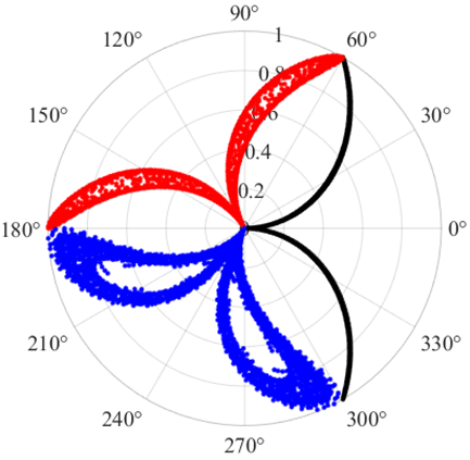
The angular magnification factor $g$ represents the angular difference between the adjacent points on the petals of the SDP image. A larger value of $g$ changes the unwrapping angle of the same pair of petals (the same channel) in the SDP image. This results in a broader petal width, which reveals additional hidden details. However, if the value of is too large, it can lead to overlap between adjacent pairs of petals, making it difficult to clearly distinguish the features. Then, to evaluate the effect of the $g$ parameter, the non-stationary signal $f_1\left(t\right)$ constructed in Section 2.1 is subjected to decomposition using JMD. The first layer of this decomposition was used as the input for the SDP, which was configured to generate a series of petals at intervals of 60º. In this framework, $\theta =60\times k$ represents the k-th pair of the generated petals. Figure 3 illustrates the corresponding SDP image for various values of the parameter $g$. It can be observed that when the value of $g$ is relatively small, each pair of petals of the same color is clearly displayed, as shown in Figure 3a,b. In contrast, as $g$ gradually increases, the image exhibits overlapping regions, which may affect the subsequent image recognition, as shown in Figure 3c,d. Thus, an appropriate $g$ value can clearly display and distinguish signals from different channels.

Different values of $l$ affect the distance between the points in polar coordinates, thereby affecting the sparsity of the petals. As the value of $l$ increases, the angle between neighboring points changes more significantly, leading to broader and sparser petals. This change enhances the visibility of detailed features of the original signal. Nevertheless, excessively large values may result in overlapping between petals. In this analysis, we set $g$ = 30, and $l$ was set to 1, 2, 4, and 8, respectively, with the same parameters $\theta$. The SDP images obtained using the different parameters are shown in Figure 4a–d. Figure 4 indicates that as parameter $l$ increases, the width of the petals gradually increases, resulting in a more pronounced and fuller appearance. In summary, to achieve a high-quality SDP pattern while minimizing petal overlap, selecting appropriate parameters can effectively accentuate the signal characteristics.

Reference [27] describes the method of manual assistance for parameter adjustment. Based on this theory and considering the overlapping of visual images and the density of petal points, this paper has determined the critical values of $g$ and $l$: $g$ = 30, $l$ = 8. While the symmetrized dot pattern (SDP) method is widely recognized as a powerful visualization tool for mechanical fault diagnosis, SDP may lose temporal information and is sensitive to parameter choices, making it less robust for signals with weak or similar fault features. Some studies have provided reference solutions: using Pearson’s correlation coefficient to quantify optimization [28], traversing parameter combinations to select the optimal parameter set [26], and using genetic algorithms to optimize parameter combinations [29], etc.

2.3. ICNN Method

In this paper, we proposed an ICNN method to address multi-class classification problems with LeakyReLU function. Its mathematical expression is $f(x)=max(0,x)+\alpha \cdot min(0,x)$, where $\alpha$ is a small positive number, and we set the negative slope $\alpha$ to 0.05. Max pooling exhibits translation invariance, meaning that it maintains important features of local regions while allowing the network to learn higher-level features [30]. In this study, to optimize the CNN architecture, max-pooling layers are strategically configured with a 2 × 2 window and a stride of 2. This pooling strategy effectively halves the size of the feature maps after each pooling operation. By doing so, it not only significantly reduces the computational demands but also minimizes the risk of overfitting. Importantly, the essential feature information is preserved, enabling the network to extract more abstract features. This enhances the model’s ability to abstractly represent images, making it more efficient and effective in learning from the data.

The entire ICNN framework adopted in this paper is illustrated in Figure 5, which comprises one image input layer, four batch normalization layers, four convolutional layers, four pooling layers, five activation functions, two fully connected layers, one SoftMax layer, and one classification layer. The size of the sample matrix for constructing the sample set is 128, so the dimension of the input data of the ICNN is 128 × 128 × 3, where 3 represents the RGB three-color channel. In this study, an activation function layer is incorporated between each convolutional layer and pooling layer, utilizing the LeakyReLU function. The output size of the fully connected layer is set to 4, indicating that four distinct signal types or labels are generated. Finally, the output was converted into a probability distribution through the SoftMax layer to complete the final classification. In this paper, MiniBatchSize is set to 32 to specify the number of samples included in each training batch, which helps to improve the utilization efficiency of the GPU. In addition, by setting MaxEpochs to 375 and InitialLearnRate to 0.001, the smaller step size makes the model more likely to stably converge to a local optimal solution or a global optimal solution during the optimization process.

2.4. Overall Process of JMD-SDP-ICNN

As previously mentioned, JMD offers excellent advantages over EMD or VMD for the extraction of jump signals. This approach can effectively decompose the characteristics of sound signals, which is beneficial for subsequent experiments. SDP further offers a clear visualization of the features at each layer following JMD decomposition. Subsequently, based on the size and number of SDP images. An ICNN was established to enable the automatic classification of these efficiently extracted fault features. Therefore, to address the issue of fault diagnosis and classification of micro-motors, this study proposes a new method based on the JMD-SDP-ICNN fault diagnosis classification model. The overall flowchart of the proposed method is illustrated in Figure 6.

The proposed method consists of the following steps: First, a sound sensor is used to collect the motor signal data with different fault states, and JMD decomposition is performed to obtain the six-layer mode decomposition results. Then, the results of the modal decomposition are visualized using SDP to construct an image library of the sound signal data. Finally, the SDP image library was divided into training and testing sets. The training dataset was used to train the ICNN model, while the test dataset was used to assess its performance. The classification results are then obtained using the trained ICNN.

3. Experimental Analysis and Verification

3.1. Experimental Setup

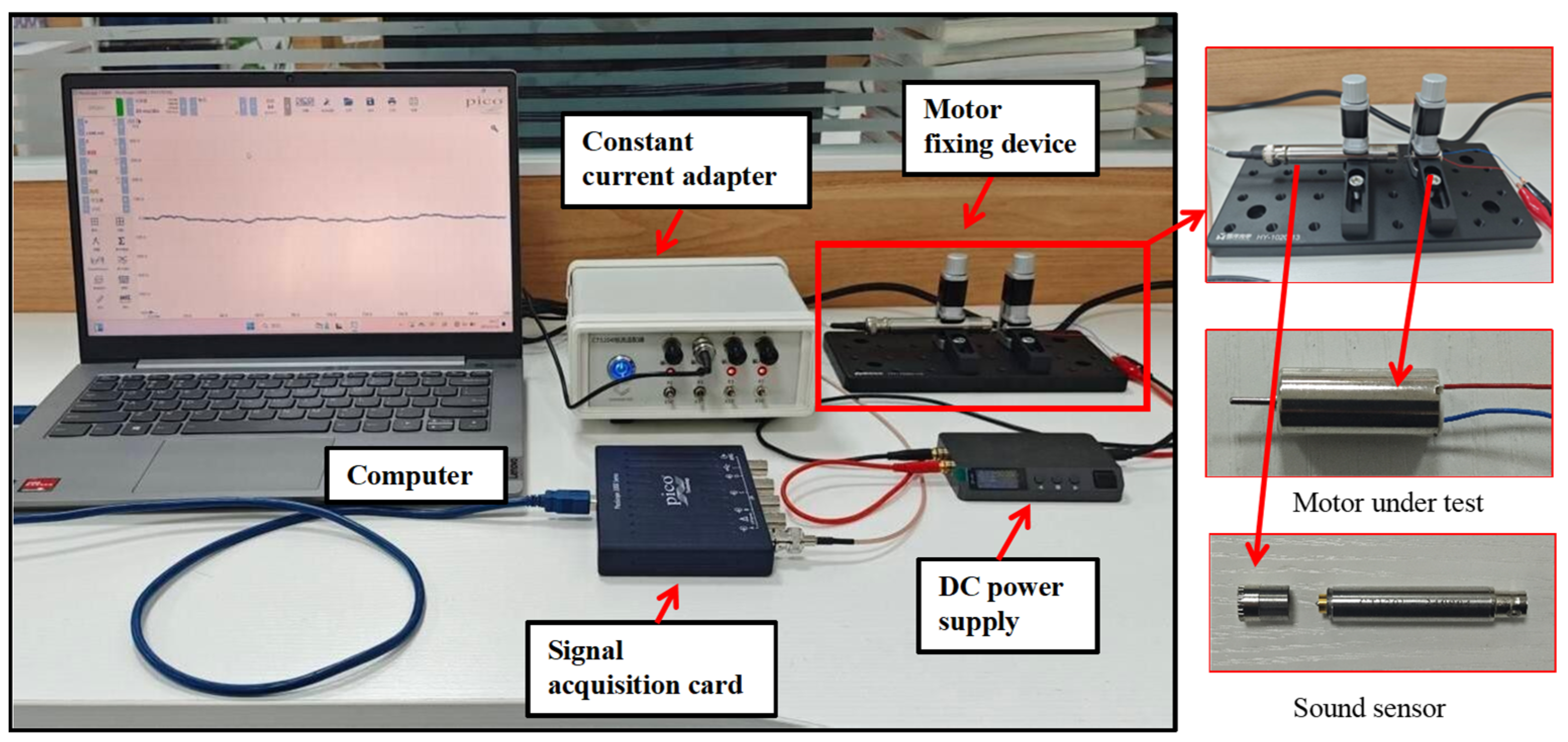
To verify the effectiveness of the proposed JMD-SDP-ICNN method, a micro-motor fault identification platform was constructed, as shown in Figure 7. The platform is mainly composed of the motor to be tested, DC power supply (DP100 numerical control power supply), sound sensor (CT1213 microphone with CT1201 amplifier, Shanghai Chengke Electronics of China), sensor adapter (CT5204 four-channel constant current adapter, Shanghai Chengke Electronics of China), signal acquisition card (PicoScope 2406 B, Pico Technology Company of UK), computer, and fixed platform. The sound sensor is capable of capturing frequencies in the range of 20 Hz to 20 kHz. The acquisition card has a bandwidth of 50 MHz and can achieve a maximum sampling rate of 1 GHz for a single active channel. The specific sample of the micro-motor used in this study was an 8520 hollow cup motor, and the detailed parameters are presented in

Table 2. Parameters of the micro-motor.

Parameters	Voltage	Current	Rotational Speed	Length	Diameter of Housing	Shaft Diameter
Value	3.7 V	150 mA	30,000 rpm	20 mm	8.5 mm	1 mm

. Throughout the experimental procedures, all motors and sound sensors were securely affixed to the fixed platform using an L-clamp.

During the experiment, the acquisition card was configured with a sampling rate of 500 kHz with a sampling duration of 2 s. Sound signals were collected from the motor under normal operating conditions and in three distinct fault states. The three fault states are (1) commutator wear (fault state A), (2) shaft bending (fault state B), and (3) housing deformation (fault state C). Multiple experiments were conducted for each condition to enhance the robustness of the data, allowing the collection of an extensive array of sample sets. The original signals were sampled in a piecewise manner to facilitate analysis.

3.2. Data Acquisition

The sound from a micro-motor can be unstable and affected by background noise. To improve its quality, we preprocess the data captured from the sound sensor. This step reduces interference and helps us extract important sound features. In this study, we focus on removing low-frequency trends from the original signal to clarify it for further analysis. Then, the preprocessed signal was decomposed by the JMD. It is crucial to set the five parameters $K$, $\alpha$, $\beta$, ${\tau }_2$, and $b$ appropriately in Equation (6) to ensure the effectiveness and convergence of the JMD decomposition. To conduct a priori analysis based on the characteristics of the signal to identify suitable values, and an adaptive strategy may be employed to dynamically adjust these parameters [31]. And in reference [11], some suggested ranges for adjusting the parameters are provided: (i) α = 10³–10⁵, (ii) 0 < β ≤ 1, (iii) τ₂ = 1.1–50, (iv) b = 0.1–0.9. Taking into account prior knowledge and the characteristics of the signal, this paper dynamically adjusted the parameters of the JMD method, and better results can be achieved with a specific set of parameters: $K=6$, $\alpha =10000$, $\beta =0.35$, $b=0.32$, ${\tau }_2=3$. It can decompose the sound signals. In this section, the sound signal is decomposed into six IMFs. Subsequently, multi-layer components are employed to multi-layer IMF components are employed to construct SDP images in this paper, which are effective in classifying various faults.

The selection of an appropriate number of decomposition variables as inputs for SDP is crucial, as it directly influences the representation of image features. Thus, to inform this selection, it is essential to analyze the importance of each IMF layer. Two key indicators for assessing the significance of the IMFs in each layer are the correlation between the decomposed signal IMFs and the original signal, along with the energy content of each IMF. To select IMFs, this study employs a correlation coefficient–energy model, $X_{\mathrm{i}}=(R_{\mathrm{i}}+E_{\mathrm{i}})/2$, where $R_{\mathrm{i}}$ is the correlation coefficient and $E_{\mathrm{i}}$ denotes the energy. The results of the six-layer decomposition parameters calculated using this formula are listed in

Table 3. Signal IMFs selection results (normal motor).

IMFs	Correlation Coefficient Ri	Energy Ei	Xi	Ranking
IMF1	0.6384	18.66%	0.4125	1
IMF2	0.3381	3.85%	0.1883	2
IMF3	0.2059	0.80%	0.1069	3
IMF4	0.1333	0.82%	0.0708	4
IMF5	0.1234	0.36%	0.0635	5
IMF6	0.0168	0.01%	0.0084	6

. From these results, the top 50% of IMFs were selected as the final signal for feature extraction in this study. Therefore, IMF1, IMF2, and IMF3 were chosen as the basis for the subsequent identification of fault conditions and served as the input for the SDP channels.

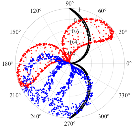
To accurately assess the occurrence of faults in the micro-motor and classify the specific fault types, this study employs three selected IMF layers as inputs for generating the SDP image. As described in Section 2.2, the parameters associated with the generation of the SDP image are determined as follows: ${\theta }_s=360 S/N$ and $S=0,1,2,\dots ,N-1$, where $N$ denotes the number of generated petals. Given that the input comprises three IMFs, $N$ is set to 3. Accordingly, the corresponding $\theta$ values for the three pairs of petals were 0, 120, and 240, respectively. Moreover, the angle amplification factor $g=60$ and the time interval coefficient $l=8$ are used to obtain non-overlapping modes. Figure 8 illustrates the SDP images for the normal motor and the three faulty motors. In these figures, the black, red, and blue petals represent IMF1, IMF2, and IMF3 components, respectively. Specifically, Figure 8a illustrates the normal condition, and Figure 8b–d correspond to commutator wear, shaft-bending fault, and housing deformation, respectively.

When comparing the images of the four working conditions of the motor shown in Figure 8, we can observe notable differences in the blue petals. Under conditions (b), (c), and (d), the blue petals exhibit an outward spread, whereas in condition (a), they converge inward. Furthermore, the black petals in conditions (b), (c), and (d) were noticeably more expansive than those in condition (a). The red petals in conditions (b), (c), and (d) display a narrower form than those in condition (a). The blue petals in (b) exhibit notable differences when compared with those in (c) and (d). Furthermore, the red petals in (c) are also distinct from those in (b) and (d). Therefore, normal and faulty micro-motors can be intuitively distinguished based on these observed differences.

4. Fault Diagnosis Analysis of Micro-Motor

The fault signal is decomposed using JMD to generate a color image, which is subsequently saved in the JPG format. A dataset of JPG images was divided into four distinct categories, specifically labeled as follows: normal, commutator wear (A fault state), shaft bending (B fault state), and housing deformation (C fault state). In this study, the sample dataset consists of 800 images, while the test dataset comprises 210 images. Then, we conducted the ICNN method mentioned in Section 2.3 for fault model learning and fault classification. This paper will verify the effectiveness of the proposed method by the following three parts:

(1)

Comparison and verification of different SDP parameter selection schemes

To validate the superiority of the SDP parameter selection in this paper, comparative experiments were conducted using several different sets of g and l values. The parameter sets selected were: (a) $g=60$, $l=8$, (b) $g=90$, $l=8$, (c) $g=90$, $l=2$, and (d) $g=60$, $l=2$. The experimental results for each parameter set are shown in

Table 4. Comparison of prediction results of different SDP paramete.

Parameter Sets	g = 60, l = 8	g = 90, l = 8	g = 90, l = 2	g = 60, l = 2
Accuracy	99.2381%	80.4762%	81.9048%	84.3809%
Schematic diagram

. When $g=90$, the petals have a certain degree of overlap, which causes some features to fail and cannot be recognized, and the final accuracy is low. When l is too small, the width of the petal is too narrow to fully display the features, and the final recognition accuracy is not satisfactory. So, we choose (a) as the values of SDP.

(2)

Comparison and verification of different decomposition approaches

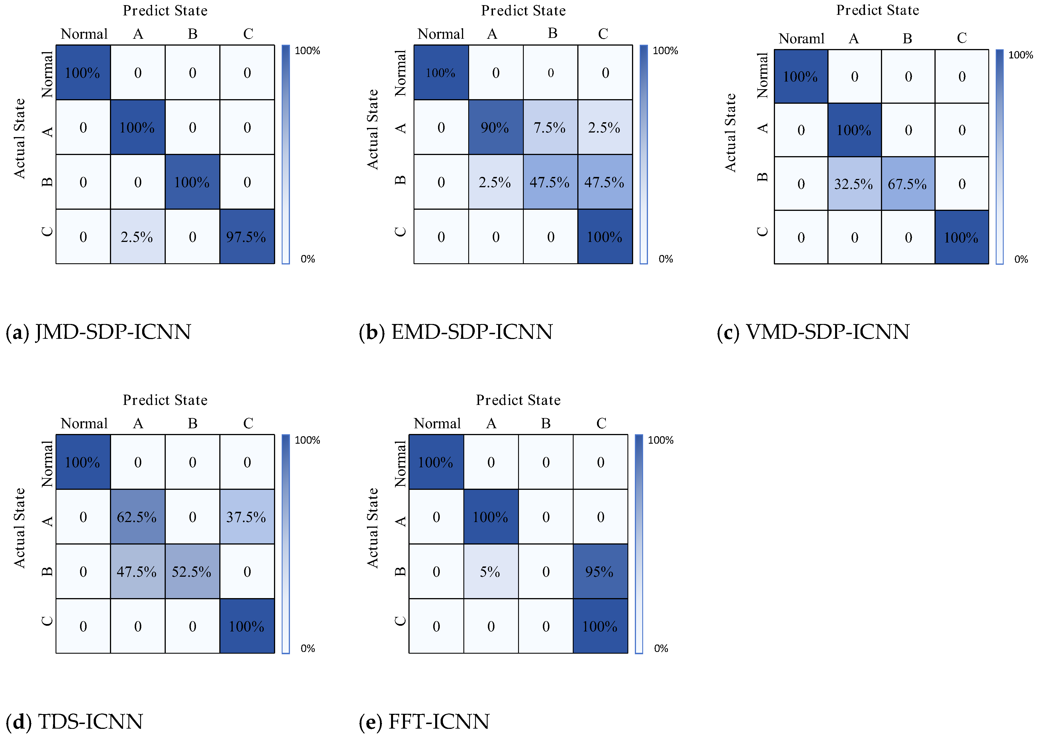
To further validate the superiority of the proposed method, we use EMD-SDP-ICNN, VMD-SDP-ICNN, TDS-ICNN (Time-Domain Signal-ICNN) and FFT-ICNN are compared with the model proposed in this paper. All methods utilize the ICNN system with identical parameters. The recognition results for the JMD-SDP-ICNN, VMD-SDP-ICNN, and EMD-SDP-ICNN are detailed in

Table 5. Comparison of prediction results of different decomposition approaches.

Models	JMD-SDP-ICNN	EMD-SDP-ICNN	VMD-SDP-ICNN	TDS-ICNN	FFT-ICNN
Accuracy	99.2381%	88.2857%	94.2857%	83.8095%	80.9524%

. The accuracy of model recognition improved significantly from 83.81% to 99.24%.

Furthermore, Figure 9 depicts the confusion matrices for these five methods, which illustrate the performance of the methods for classifying motor fault states. The vertical axis delineates the actual labels associated with the test set samples, and the horizontal axis indicates the labels predicted by the model. The figures reveal that the JMD-SDP-ICNN method can completely classify the normal, A, and B fault states into their respective categories, and the identification of the C fault state also achieves a high accuracy rate. Additionally, the EMD-SDP-ICNN approach exhibits a significantly low recognition accuracy of only 47.5% for fault state B, which misclassifies a significant number of shaft bends as commutator wear. In contrast, the VMD-SDP-ICNN approach misclassifies a certain amount of shaft bends as commutator wear. For TDS-ICNN, the confusion between fault states A and B is very serious because the input signal is not processed. However, FFT-ICNN fails to identify fault state B. Compared with other methods, the proposed JMD-SDP-CNN method achieved superior accuracy and a better diagnostic effect in diagnosing fault types and missing faults.

(3)

Comparison and verification of different trained models

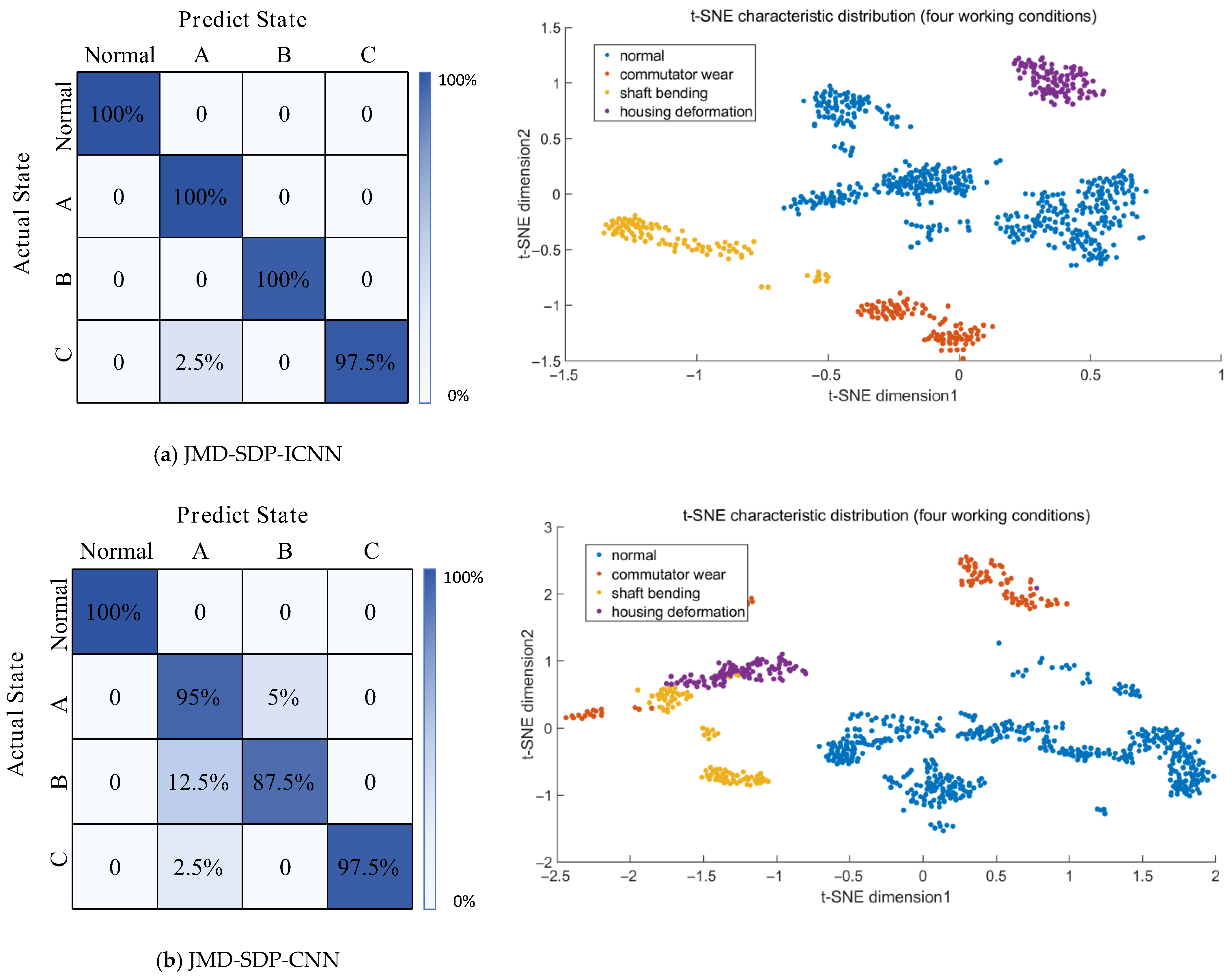
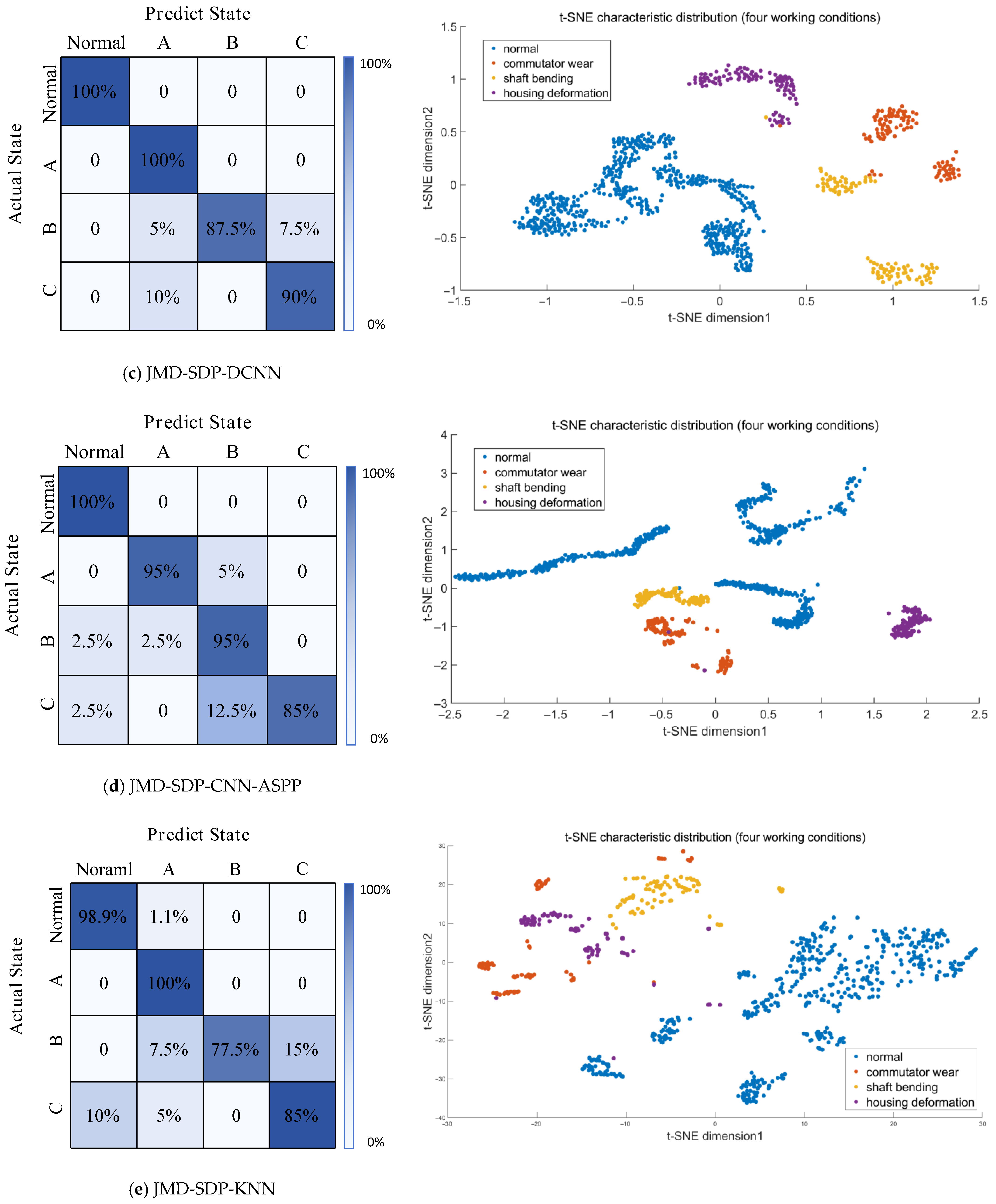
To evaluate the accuracy of the ICNN training, image data from the sample set were systematically input into five distinct classification models: ICNN, CNN, DCNN (Deep Convolutional Neural Network), CNN-ASPP (Convolutional Neural Network–Atrous Spatial Pyramid Pooling), and K-Nearest Neighbor (KNN). A comparative analysis was conducted on the recognition performances of the SDP-CNN, SDP-KNN, and SDP-SVM models. The results of the experimental predictions and training time are listed in

Table 6. Comparison of prediction results of different trained models.

Models	Accuracy	Training Time (s)	Number of Iterations
JMD-SDP-ICNN	99.2381%	10	375
JMD-SDP-CNN	94.9424%	14	250
JMD-SDP-DCNN	97.5238%	37	250
JMD-SDP-CNN-ASPP	95.3333%	141	1500
JMD-SDP-KNN	92.3810%	22	/

. It can be seen from the table that ICNN takes less time than CNN and DCNN with more iterations; this advantage means that the model proposed in this paper will be adapted to more industrial scenarios. At the same time, the recognition accuracy of JMD-SDP-ICNN for different working conditions reaches 99.2381%, which is better than other methods.

The confusion matrices identified by different models for the four working conditions and the t-SNE plot are shown in Figure 10. As can be seen in this figure, JMD-SDP-ICNN has high accuracy in the recognition of four working conditions, and the distribution boundaries of features in different working conditions are clear, which is significantly better than other models.

(4)

Comparison and verification of another public dataset

To further verify the practicality and robustness of the proposed model, the bearing fault public datasets from Case Western Reserve University (CWRU) were used for performance validation. Specifically, four working conditions—normal, inner race fault, ball fault, and outer race fault—under no-load conditions, rotational speed of 1797 rpm, and fault diameter of 0.007” were selected as the original data. The classification task was conducted for these four conditions. After manual-assisted optimization, the JMD parameters were determined as follows: $K=6$, $\alpha =100000$, $\beta =0.86$, $b=0.35$, ${\tau }_2=1.1$. The classification accuracy results are presented in

Table 7. Comparison of prediction results of the public dataset.

Models	JMD-SDP-ICNN	JMD-SDP-CNN	JMD-SDP-DCNN	JMD-CNN-ASPP	JMD-KNN
Accuracy	99.9091%	98.6364%	98.8182%	98.0909%	96.3636%

. Figure 11 displays the confusion matrix and t-SNE plots of the classification results for each model. As shown in the table and figures, the proposed model demonstrates excellent classification performance and robustness.

5. Conclusions

In this paper, we propose a novel method for micro-motor fault diagnosis based on JMD-SDP-ICNN. By employing a multi-level signal processing and feature extraction framework, this approach significantly improves the ability to extract features from weak acoustic signals, achieving the accuracy and rate of identifying various fault types.

(1)

Firstly, the JMD method was employed to effectively solve the problem of signal aliasing, which is often encountered in traditional signal processing. This method offers distinct advantages, particularly in handling jump signals. By constructing non-stationary signals for verification, it is demonstrated that the method is especially suitable for separating characteristic components of motor fault signals.

(2)

Secondly, the multi-channel SDP visualization method was introduced to effectively convert the selected IMF components into 2D faulty petal images in polar space. This technique enhances the clarity of signal features and supports intuitive fault classification.

(3)

At last, we proposed an ICNN method with the LeakyReLU activation function to replace the traditional CNN to identify SDP images. This modification allows the network to continue receiving gradient updates even when it encounters negative inputs during training, ultimately enhancing the stability and performance of the fault type identification model.

(4)

The ICNN fault classification model was used to classify the generated SDP images efficiently. Through experimental verification, this method performs well in multiple fault classification tests, and the accuracy rates on the self-built platform and the CWRU public dataset reached 99.2381% and 99.9091%, respectively, which has significant advantages compared with other methods.

This method overcomes the reliance on high-precision sensors that are typically required for traditional vibration detection. Instead, it utilizes low-cost acoustic signals to diagnose multiple faults in micro-motors accurately. Future research will focus on refining this approach to better accommodate more complex industrial scenarios and meet higher accuracy requirements for fault diagnosis.

References

1. Zhao, H.; Ye, M.; Nelson, B.J.; Wang, X. A Selectively Controllable Triple-Helical Micromotor. IEEE Robot. Autom. Lett. 2024, 9, 4742–4749. [Google Scholar] [CrossRef]
2. Niu, Y.; Jin, X.; Wen, Z. Research on Command and Control Technology in Small-UAV Defense System. In Proceedings of the 2021 International Conference on Computer Information Science and Artificial Intelligence, Kunming, China, 17–19 September 2021; pp. 673–677. [Google Scholar] [CrossRef]
3. Sawa, K.; Ueno, T.; Nakano, K.; Toya, K. Effects of Brush Spring Force on Brush Wear and Arc Behaviors of Small DC Motor. In Proceedings of the 2023 IEEE 68th Holm Conference on Electrical Contacts (HOLM), Seattle, WA, USA, 4–11 October 2023; pp. 1–6. [Google Scholar] [CrossRef]
4. Gretskov, A.; Boyarkina, U.; Vorokh, D. Application of Radio-Wave Motion Transducers to Measure the Parameters of Bending Vibrations of a Turbine Unit Shaft. In Proceedings of the 2024 IEEE Ural-Siberian Conference on Biomedical Engineering, Radioelectronics and Information Technology (USBEREIT), Yekaterinburg, Russia, 13–15 May 2024; pp. 241–244. [Google Scholar] [CrossRef]
5. Wu, J.; Xu, Q.; Xu, L. A Study on Winding MMF Harmonic and Vibration of Polyphase Motor. In Proceedings of the 2021 Power System and Green Energy Conference (PSGEC), Shanghai, China, 20–22 August 2021; pp. 732–737. [Google Scholar] [CrossRef]
6. Javorskyj, I.; Yuzefovych, R.; Lychak, O.; Trokhym, G.; Varyvoda, M. Methods of Periodically Non-Stationary Random Processes for Vibrations Monitoring of Rolling Bearing with Damaged Outer Race. Digit. Signal Process. 2024, 145, 104343. [Google Scholar] [CrossRef]
7. Han, J.; Song, J.H. Phase Current-Balance Control Using DC-Link Current Sensor for Multiphase Converters with Discontinuous Current Mode Considered. IEEE Trans. Ind. Electron. 2016, 63, 4020–4030. [Google Scholar] [CrossRef]
8. Chen, C.; Li, H.; Feng, Y.; Chen, J.; Cai, S.; Yin, J. Research on Low Temperature Characteristics and Application of Temperature Sensor in Alpine Region. In Proceedings of the 2022 IEEE 5th International Electrical and Energy Conference (CIEEC), Nangjing, China, 27–29 May 2022; pp. 1551–1556. [Google Scholar] [CrossRef]
9. Gu, J.; Peng, Y. An Improved Complementary Ensemble Empirical Mode Decomposition Method and Its Application in Rolling Bearing Fault Diagnosis. Digit. Signal Process. 2021, 113, 103050. [Google Scholar] [CrossRef]
10. Chen, J.; Li, S.; Zhu, J.; Liu, M.; Li, R.; Cui, X.; Li, L. Significant Wave Height Prediction Based on Variational Mode Decomposition and Dual Network Model. Ocean Eng. 2025, 323, 120533. [Google Scholar] [CrossRef]
11. Nazari, M.; Korshøj, A.R.; ur Rehman, N. Jump Plus AM-FM Mode Decomposition. IEEE Trans. Signal Process 2024, 73, 1081–1093. [Google Scholar] [CrossRef]
12. Gbashi, S.M.; Adedeji, P.A.; Olatunji, O.O.; Madushele, N. Optimal Feature Selection for a Weighted K-Nearest Neighbors for Compound Fault Classification in Wind Turbine Gearbox. Results Eng. 2025, 25, 103791. [Google Scholar] [CrossRef]
13. Ren, H.; Liu, S.; Qiu, B.; Guo, H.; Zhao, D. A Novel Intelligent Fault Diagnosis Method of Bearing Based on Multi-Head Self-Attention Convolutional Neural Network. Artif. Intell. Eng. Des. Anal. Manuf. AIEDAM 2024, 38, e9. [Google Scholar] [CrossRef]
14. Pickover, C.A. On the use of symmetrized dot patterns for the visual characterization of speech waveforms and other sampled data. J. Acoust. Soc. Am. 1986, 80, 955–960. [Google Scholar] [CrossRef]
15. Xian, X.; Tang, H.; Tian, Y.; Liu, Q.; Fan, Y. Performance Analysis of Different Machine Learning Algorithms for Identifying and Classifying the Failures of Traction Motors. J. Phys. Conf. Ser. 2021, 2095, 012058. [Google Scholar] [CrossRef]
16. Zhu, X.; Hou, D.; Zhou, P.; Han, Z.; Yuan, Y.; Zhou, W.; Yin, Q. Rotor Fault Diagnosis Using a Convolutional Neural Network with Symmetrized Dot Pattern Images. Meas. J. Int. Meas. Confed. 2019, 138, 526–535. [Google Scholar] [CrossRef]
17. Rani, S.; Memoria, M.; Almogren, A.; Bharany, S.; Joshi, K.; Altameem, A.; Rehman, A.U.; Hamam, H. Deep Learning to Combat Knee Osteoarthritis and Severity Assessment by Using CNN-Based Classification. BMC Musculoskelet. Disord. 2024, 25, 817. [Google Scholar] [CrossRef] [PubMed]
18. Goh, K.W.; Surono, S.; Afiatin, M.Y.F.; Mahmudah, K.R.; Irsalinda, N.; Chaimanee, M.; Onn, C.W. Comparison of Activation Functions in Convolutional Neural Network for Poisson Noisy Image Classification. Emerg. Sci. J. 2024, 8, 592–602. [Google Scholar] [CrossRef]
19. Wang, L.H.; Zhao, X.P.; Wu, J.X.; Xie, Y.Y.; Zhang, Y.H. Motor Fault Diagnosis Based on Short-Time Fourier Transform and Convolutional Neural Network. Chin. J. Mech. Eng. 2017, 30, 1357–1368. [Google Scholar] [CrossRef]
20. Xing, Y.; Li, H. Rolling Bearing Fault Diagnosis Based on Model Migration. In Intelligent Computing Theories and Application; Lecture Notes in Computer Science; Springer Nature: Berlin, Germany, 2022; Volume 13393, pp. 135–146. [Google Scholar] [CrossRef]
21. Dragomiretskiy, K.; Zosso, D. Variational Mode Decomposition. IEEE Trans. Signal Process. 2014, 62, 531–544. [Google Scholar] [CrossRef]
22. Zhang, C.H. Nearly Unbiased Variable Selection Under Minimax Concave Penalty. Ann. Stat. 2010, 38, 894–942. [Google Scholar] [CrossRef]
23. Cicone, A.; Huska, M.; Kang, S.H.; Morigi, S. JOT: A Variational Signal Decomposition into Jump, Oscillation and Trend. IEEE Trans. Signal Process. 2022, 70, 772–784. [Google Scholar] [CrossRef]
24. Wu, B.; Tang, W.; Zhou, Z.; Tan, Y.; Chen, S.; Feng, Y. An Improved Adaptive EMD-SVD Method for Railway Bridge Dynamic LG-Strain Processing under Moving Trainloads. Structures 2025, 80, 109777. [Google Scholar] [CrossRef]
25. Long, Z.; Guo, J.; Ma, X.; Wu, G.; Rao, Z.; Zhang, X.; Xu, Z. Motor Fault Diagnosis Based on Multisensor-Driven Visual Information Fusion. ISA Trans. 2024, 155, 524–535. [Google Scholar] [CrossRef]
26. González, J.; Oro, J.M.F.; Delgado, L.; Méndez, D.; Argüelles, K.M.; Velarde-suárez, S.; Rodríguez, D. Symmetrized Dot Pattern Analysis for the Unsteady Vibration State in a Sirocco Fan Unit. Appl. Acoust. 2019, 152, 1–12. [Google Scholar] [CrossRef]
27. Xu, X.; Liu, H.; Zhu, H.; Wang, S. Fan Fault Diagnosis Based on Symmetrized Dot Pattern Analysis and Image Matching. J. Sound Vib. 2016, 374, 297–311. [Google Scholar] [CrossRef]
28. Gu, Y.; Zeng, L.; Qiu, G. Bearing Fault Diagnosis with Varying Conditions Using Angular Domain Resampling Technology, SDP and DCNN. Measurement 2020, 156, 107616. [Google Scholar] [CrossRef]
29. Zhang, C.; Wang, W.; Li, H. Tool Wear Prediction Method Based on Symmetrized Dot Pattern and Multi-Covariance Gaussian Process Regression. Measurement 2022, 189, 110466. [Google Scholar] [CrossRef]
30. Shiney, S.A.; Seetharaman, R.; Sharmila, V.J.; Prathiba, S. Deep Learning Based Gasket Fault Detection: A CNN Approach. Sci. Rep. 2025, 15, 4776. [Google Scholar] [CrossRef] [PubMed]
31. Li, H.; Liu, T.; Wu, X.; Chen, Q. An Optimized VMD Method and Its Applications in Bearing Fault Diagnosis. Measurement 2020, 166, 108185. [Google Scholar] [CrossRef]
Figure 1. Comparison of JMD, EMD, and VMD decomposition for the same signal, the dashed black lines represent the original components of the signal, while the red, green, and blue solid lines represent the decomposition results of JMD, EMD, and VMD, respectively.
Actuators 14 00405 g001
Figure 2. Comparison of the frequency spectrum of the oscillatory components obtained by JMD, EMD, and VMD decomposition.
Actuators 14 00405 g002
Figure 3. Effect of parameter g variation on SDP image, red, green, black, yellow, purple and blue represent petals of 0°, 60°, 120°, 180°, 240° and 300°, respectively.
Actuators 14 00405 g003
Figure 4. Effect of parameter l variation on SDP image, red, green, black, yellow, purple and blue represent petals of 0°, 60°, 120°, 180°, 240° and 300°, respectively.
Actuators 14 00405 g004
Figure 5. The entire ICNN framework for fault classification.
Actuators 14 00405 g005
Figure 6. Overall flowchart of fault diagnosis classification by proposed JMD-SDP-ICNN.
Actuators 14 00405 g006
Figure 7. Micro-motor sound signal acquisition platform.
Actuators 14 00405 g007
Figure 8. SDP images under different working conditions, black, red and blue petals represent IMF1, IMF2 and IMF3, respectively.
Actuators 14 00405 g008
Figure 9. Prediction results of four working conditions for three models in a training session, (ac) represent commutator wear, shaft bending, and housing deformation.
Actuators 14 00405 g009
Figure 10. Confusion matrix and t-SNE plot of the recognition results of different models (the legends of normal, commutator wear, shaft bending, and housing deformation are blue, orange, yellow, and purple, respectively).
Actuators 14 00405 g010aActuators 14 00405 g010b
Figure 11. Confusion matrix and t-SNE plot of the recognition results of different models (the legends of normal, inner race fault, ball fault, and outer race fault are blue, orange, yellow, and purple, respectively).
Actuators 14 00405 g011aActuators 14 00405 g011b