1. Introduction
Permanent magnet synchronous motors (PMSMs) exhibit superior attributes such as high efficiency, power density, and precision controllability [
1,
2]. These advantages have contributed to the widespread adoption of PMSMs in various fields, including industrial automation, transportation, and home appliances. As performance indicators such as power density, overload capacity, and lightweight design continue to improve, the electromagnetic load on the motor also increases, leading to a corresponding rise in vibration intensity [
3,
4,
5]. Moreover, the motor’s performance can be severely compromised when exposed to high temperatures for extended periods, as limited installation space and inadequate heat dissipation can lead to the degradation of the permanent magnets. Therefore, ensuring safe and reliable operation of permanent magnet synchronous motors (PMSMs) remains a critical industrial priority, driving accelerated interdisciplinary research in design optimization.
Reducing torque ripple is critical for enhancing the operational smoothness, vibration, and noise performance of permanent magnet and reluctance motors, driving research into various solutions based on electromagnetic design optimization and control strategies. Rafaq et al. [
6] systematically investigated torque ripple generation mechanisms and proposed a current waveform modulation strategy for effective suppression; Yamashita et al. [
7], focusing on synchronous reluctance motors, combined iron loss sensitivity analysis using the adjoint variable method with topology optimization via the level set method to improve torque characteristics while minimizing iron losses.
Research has been focusing on optimizing diverse structural parameters to achieve high efficiency, high torque, and robust operation. For instance, Xing and Zezhic [
8] studied a 60-slot/4-pole IPMSM with a non-uniform air gap, systematically considering geometric structure, permanent magnet (PM) arrangement, and rotor flux barrier design. They proposed an optimization method to achieve the optimal PM arrangement for a U-shaped rotor, successfully reducing both torque ripple and electromagnetic vibration intensity. Naik et al. [
9] applied the meta-heuristic Rao algorithm combined with the finite element method to investigate the impact of air gap magnetic flux density, electromagnetic torque, and flux density on IPMSM efficiency under varying stator slot configurations and operating conditions. Zhu et al. [
10] conducted topology optimization on dual-armature flux-switched permanent magnet (DA-FSPM) motors (featuring U-type, E-type, and C-type), performing detailed parameter analysis encompassing copper loss distribution, magnetic pole radius, stator tooth radius, and yoke thicknesses to maximize average torque. Furthermore, Reyes et al. [
11] highlighted the influence of input parameter uncertainty on motor performance and employed a 2D finite element surrogate model for the robust optimization design of permanent magnet-assisted synchronous reluctance motors. Their study demonstrated the necessity of robust strategies for achieving both optimal and stable performance under consistent operating conditions. Collectively, these studies illustrate that PMSM design optimization is a complex, multi-parameter, multi-objective process spanning geometry, materials, electromagnetics, and control, requiring simultaneous consideration of deterministic performance and robustness.
In multi-objective optimization studies, the complex nonlinear relationships between design variables and objective functions necessitate the development of accurate mathematical models, which are critical for effective problem-solving. Significant efforts have thus been dedicated to high-precision modeling techniques [
12,
13,
14]. Xu et al. [
15] established a mathematical model for the built-in PMSM used in traction drives. They conducted a multi-objective optimization design based on flat wire winding technology, which effectively suppressed torque ripple and validated the proposed methodology; Sun et al. [
16], addressing the dynamic performance and energy consumption of PMSMs under complex operating conditions, developed a finite element characterization method using equivalent points on the speed–torque plane and proposed a multi-objective structural optimization method to simultaneously reduce torque ripple and energy consumption. To address computational burden, Kim et al. [
17] proposed an adaptive response surface method that minimizes finite element evaluations required for determining the response surface parameters. By optimizing computation time based on the structure of the computing cluster, this method enabled efficient reliability evaluation of power electronic modules; Zhang et al. [
18] integrated adaptive response surfaces with a Gaussian global harmony search algorithm into a double-loop framework, demonstrating its global optimization capability using NASA aircraft stiffener plates.
Current research on PMSM performance enhancement primarily emphasizes single-dimensional approaches—whether through structural topology optimization, electromagnetic theory refinement, or advanced control techniques. While effective for specific performance metrics, these conventional methods often neglect synergistic improvements across multiple operational parameters. To bridge this critical gap, this investigation establishes a comprehensive optimization framework through systematic analysis of a 12-pole/36-slot built-in PMSM.
The main contributions of the study are as follows:
We conduct large-scale exploration of the design space through DOE sampling, making large-scale exploration of the interaction between electromagnetic structures possible.
Leveraging sampling data obtained from large-scale design space exploration via design of experiments (DOE), we develop a high-fidelity predictive metamodel that closely approximates the actual system’s behavior.
Sensitivity analysis is conducted on critical optimization design parameters to identify those exhibiting the highest sensitivity to the target performance metrics, which are subsequently selected as primary design variables.
The proposed methodology not only enhances the output torque, but also achieves concurrent reductions in stator core loss, torque ripple, and radial electromagnetic force, thereby delivering a significant improvement in overall motor performance efficiency.
2. The Best Predictive Metamodel for PMSM
The Moving Least Squares (MLS) method employs kernel-based weighting to prioritize proximal data points for localized approximation. Enhanced by an AMLS approach, this framework dynamically adjusts weight functions, basis functions, and algorithm parameters in response to local data characteristics, noise levels, and cross-validation metrics.
The optimal adaptive metamodel is constructed via MFS-MLS methodology, integrating Moving Frame Method with Moving Least Squares. The MFS-MLS methodology was selected owing to its distinctive capabilities in addressing PMSM-specific optimization challenges, characterized by three key features:
Local Adaptability: Achieved via an adaptive moving-window mechanism employing modified Gaussian weighting functions (refer to
Section 2), which facilitates a dynamic response to localized nonlinearities within electromagnetic field distributions, crucial for accurately capturing abrupt variations in torque ripple and radial force density.
Computational Efficiency: Attained through the resolution of localized least-squares problems (refer to Equations (8)–(11)), this approach obviates the need for computationally burdensome inversions of large-scale covariance matrices, as required in Gaussian processes, thereby diminishing computational overhead in high-dimensional design spaces (e.g., 7 variables as indicated in
Table 1).
Multi-Fidelity: Integration facilitated by scaling function a0(x) (Equation (2)) to incorporate low-fidelity data, a capability absent in pure interpolation methods such as radial basis functions (RBFs).
For the sampled data point set {(
xi,
yi)}, the error is minimized by fitting a polynomial function
P(
x) to approximate the true model. The polynomial model’s predicted response
P(x) is mathematically expressed as:
where
x represents the vector of design variables within the n-dimensional design space, and
denote the polynomial coefficients. To overcome limitations of conventional regression methods, this work develops an MFS-MLS model.
The high-precision prediction metamodel for PMSM, constructed using the MLS method, acknowledges that not all sample points hold equal significance when estimating the regression coefficients. Therefore, when constructing the loss function, each squared residual is assigned a weight that varies based on the distance between the point to be predicted and each observed data point. Moreover, the coefficients of the moving least squares model are functions of the input x. At each predicted point x_new, the coefficients are computed using the sample points within the neighborhood of x_new. This neighborhood defines the influence domain of the point x_new, with sample points outside this domain being excluded. As the prediction point moves, the influence domain adjusts accordingly.
This approach enables the high-fidelity analysis model to automatically determine both the size of the influence domain based on the sample points and the varying scale factors of the predicted points, providing enhanced flexibility and accuracy. The expression is mathematically defined as follows [
19]:
where
is a function of the design variable
X,
is the scaling function of the low-fidelity model
, and
is the coefficient of the basis function. The coefficient vector is augmented to form the equation that includes
and
,
Here, m represents the number of terms in the basis function. The term
is defined as the difference function.
is a monomial basis function, which is extended to form the integrated vector
.
In the absence of specific knowledge about the properties of real functions, linear and quadratic polynomials are typically used as basic functions [
20]. A complete quadratic basis function can be written as
. Therefore, the ensemble vector
can be expressed as
. To compute the coefficient vector
, an objective function
, consisting of weighted discrete
norms, must be minimized.
where
represents the
high-fidelity sampling points near the evaluation point
, and
is the weighting function applied to the samples.
Equation (3) is expressed in matrix form as
where
with
Taking the derivative of Equation (4) with respect to a(x) and setting it to zero yields:
where
Consequently, the solution for a(x) is:
Substituting a(x) back into Equation (2), we obtain the estimated response:
As shown in Equation (11), the parameter k is adjusted to control the decay speed of the Gaussian weight function , which represents the weight of each sample point. This adjustment allows the model to better adapt to varying data distributions and enhances fitting accuracy.
The Gaussian weight function is given by [
21]:
where
is a constant influencing the effect of the Euclidean distance between points
x and
, and
are the standard deviation of the Gaussian distribution.
3. The Kriging Surrogate Model
In multidisciplinary and multi-objective optimization, the relationship between dependent and independent variables is explored using surrogate modeling. Surrogate modeling has become an indispensable tool across engineering, scientific, and economic domains for approximating complex simulations and experimental processes, enabling accelerated computation, cost reduction, and data-driven optimization. Among prevalent surrogate techniques—including polynomial regression, support vector machines, and neural networks—the Kriging model distinguishes itself through its capacity to provide minimum-variance unbiased predictions while delivering quantitative uncertainty estimates.
The Kriging framework assumes stationarity, where the covariance between any two points depends solely on their spatial separation rather than absolute position:
where
denotes the covariance kernel function.
The goal of Kriging interpolation is to determine a set of weighting coefficients that minimize the prediction error
, which can be expressed as follows:
where
is the weighting coefficient;
is the objective function value at the known data point
.
The weighting coefficients are determined by solving the Kriging equation
where C is the covariance matrix between training samples, λ is the weight vector, and
is the covariance vector between the prediction point
and training data.
The coefficient of determination is an index used to assess the fitting accuracy of a polynomial regression model. It is defined as the percentage of variation explained by the fitted value of the response parameter, with its value ranging from 0 to 1. The closer the value is to 1, the better the model’s fitting performance. Its expression is:
where the sum of squared residuals
is the sum of the squared differences between the observed and predicted values;
is the total sum of squares, representing the sum of the squared differences between the observations and the mean of the observations.
Considering models of varying complexity, the adjusted coefficient of determination
is expressed as
where
n is the number of samples and m is the number of independent variables.
In the study, the sample space is partitioned, and the coefficient of determination is calculated using the cross-validation algorithm. The predicted values
are obtained through the regression model. By evaluating and combining the predictive qualities of both the interpolation and regression models, the optimal adaptive meta-model that meets the required criteria is determined based on the coefficient of determination. As shown in
Figure 1, the predicted coefficients for total COP all reached over 90%, meeting the high precision requirement for a multi-objective optimization problem.
4. Sensitivity Analysis
Table 2 lists the key structural parameters of the motor under study in this paper.
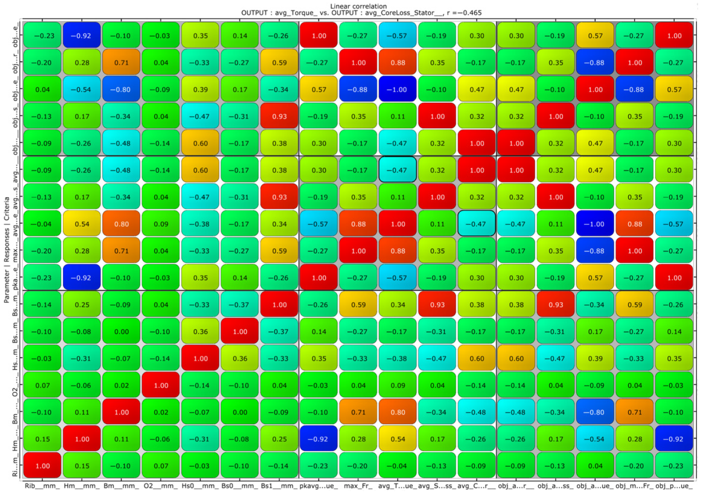
In the optimal predictive adaptive metamodel, uncertainty in the input parameters may lead to uncertainty in the model output parameters. To further improve the quality of the best fit, sensitivity analysis is essential prior to conducting the multi-objective optimization design, which employs local gradient-based derivatives to assess the primary influence of design variables on motor performance. This approach is suitable due to the approximately linear relationship observed between key motor performance and structural parameters within the optimized design domain, reducing the need for higher-order sensitivity analysis. Further, the inherent ability of the multi-objective optimization algorithm to explore interactions via Pareto solutions compensates for the relative simplicity of this sensitivity method. Additionally, the tenfold increase in samples required for Sobol indices compared to gradient-based methods was deemed prohibitively expensive given Finite Element Method simulation costs. The correlation coefficients in
Figure 2 represent normalized partial derivatives; their sign indicates the influence direction (e.g., increasing B
m decreases torque ripple but increases radial force). The correlation coefficient between the optimization variables and the objective function f is defined as follows.
where
is the j-th optimization variable, and
represents the correlation coefficient between
and f.
The structural parameters of the motor are shown in
Figure 3. Based on previous research, torque ripple, stator core loss, electromagnetic force amplitude, and output average torque are chosen as the performance optimization objectives. The key structural parameters that influence the motor’s performance, such as slot width
Bs0, slot heart width
Bs1, slot height
Hs0, permanent magnet width
Hm, slot spacing Rib between adjacent poles, distance
O2 between the bottom of the permanent magnet and the inner circle of the rotor, and permanent magnet thickness
, are selected as the optimization design variables. The initial values and ranges of the variables initially selected in the experimental design are presented in
Table 1. Design variable boundaries in multi-objective optimization are defined by physical constraints and electromagnetic viability. As
Table 1 shows, physical constraints set mechanical integrity lower bounds and saturation prevention upper bounds to avoid lamination distortion during stamping. Electromagnetic constraints limit flux leakage while maintaining greater than 70% slot-fill factor for feasible winding.
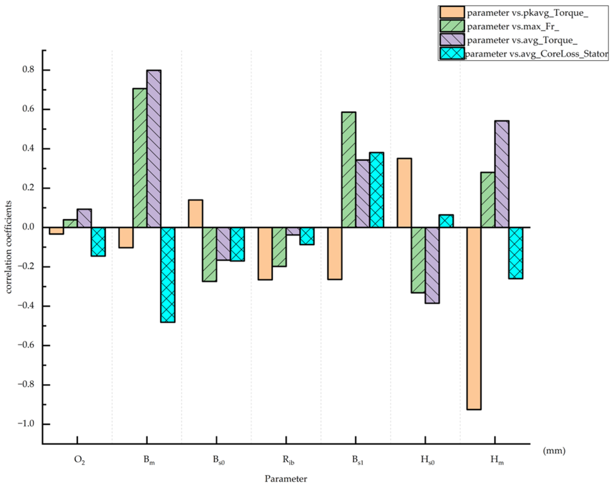
Sensitivity analysis was performed on the four objectives concerning the seven design variables, yielding the correlation coefficients between the optimization objectives and design variables, as shown in
Figure 3. The positive and negative signs of the sensitivity coefficients indicate the direction of the correlation between the parameters and the objectives. Specifically, a positive coefficient indicates a positive correlation, while a negative coefficient indicates a negative correlation. The absolute value of the sensitivity coefficient reflects the magnitude of the influence that parameter changes have on the optimization objective. The larger the absolute value, the more significant the influence of the parameter on the objective.
Figure 4 demonstrates notable differences in the sensitivities of various design variables across the objectives. For instance, stator core loss is predominantly affected by the slot height
Hs0, slot core width
Bs1, and permanent magnet thickness
Bm, while it is less affected by the slot width
Bs0 and the distance between the magnet bottom and the inner rotor circle. The output torque is influenced not only by the permanent magnet thickness
Bm and permanent magnet width
Hm, but also by the slot height
Hs0 and slot core width
Bs1. The variables that have the greatest impact on the radial electromagnetic force are the permanent magnet thickness
Bm and the slot core width
Bs1; while torque ripple is primarily dependent on the magnet width
Hm, it is also affected by
Hs0,
Bs1, and the slot spacing
Rib of the magnets at adjacent poles.
This is largely because the slot spacing between adjacent magnets influences the harmonic distribution of the air-gap magnetic field in the permanent magnet synchronous motor, along with factors such as the rotor distance O2 and the slot spacing Rib between adjacent poles.
5. Multi-Objective Optimization Model of PMSM Performance
Based on the results of the sensitivity analysis, the selected optimization design variables are the permanent magnet thickness
Bm, permanent magnet width
Hm, slot height
Hs0, and slot core width
Bs1. The optimized parameters of the multi-objective genetic algorithm (MOGA) are listed in
Table 2, with their formulation as follows:
where
avg(CoreLoss(stator)) is the average value of the stator core loss of the motor under rated operating conditions,
avg(Torque) is the average output torque,
pkavg(Torque) represents the torque ripple, and
max(Fr) denotes the peak amplitude of the radial electromagnetic force.
The efficacy of NSGA-II is substantially contingent upon the initial parameters, as evidenced in
Table 3. The population size N necessitates a proportional adjustment in accordance with the objective dimension M and the design variables D. In the context of this study, which encompasses four objectives (M = 4) and four design variables (D = 4), the minimum population size Nmin is established at 64, though empirically expanded to 100 to augment diversity. The maximum permissible percentage of the Pareto front is increased to 20% to preserve a distribution of trade-off solutions. To mitigate the sparsity of solutions in high-dimensional spaces, to improve the efficiency of global search, and to avoid local entrapment, the crossover probability is fixed at 0.95. The maximum iteration count and the mutation probability are pivotal factors that influence computational efficiency, convergence of solutions, and the quality of optimization. These parameters necessitate a thorough evaluation, taking into account the complexity of the problem, the size of the population, the computational resources available, the landscape of the objectives, and the rate of change of the Pareto front. Consequently, the maximum iteration count is set at 60, with the mutation probability at 0.05. Based on sensitivity analysis, parameters such as slot width and permanent magnet thickness exhibit a high degree of sensitivity with respect to torque and iron loss. Therefore, the percentage stability is configured at 70.
The response surfaces in
Figure 5,
Figure 6 and
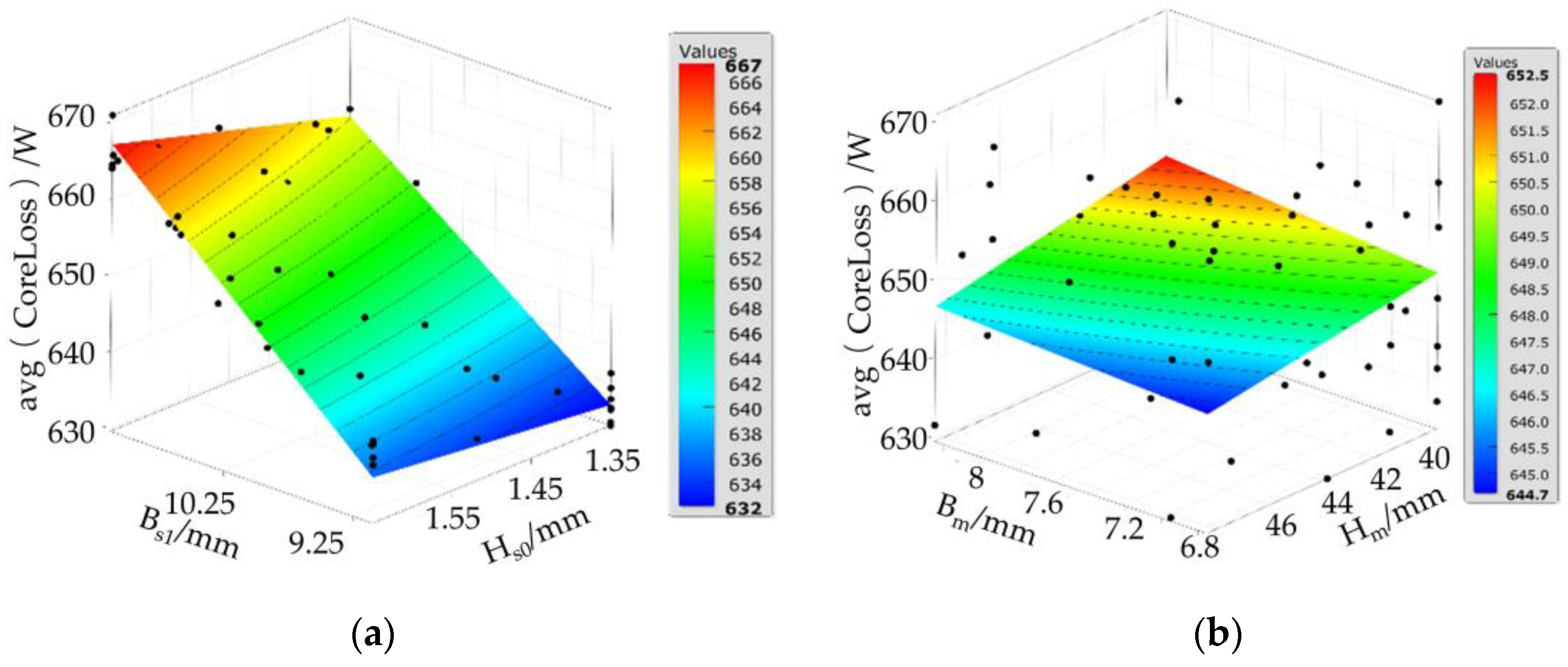
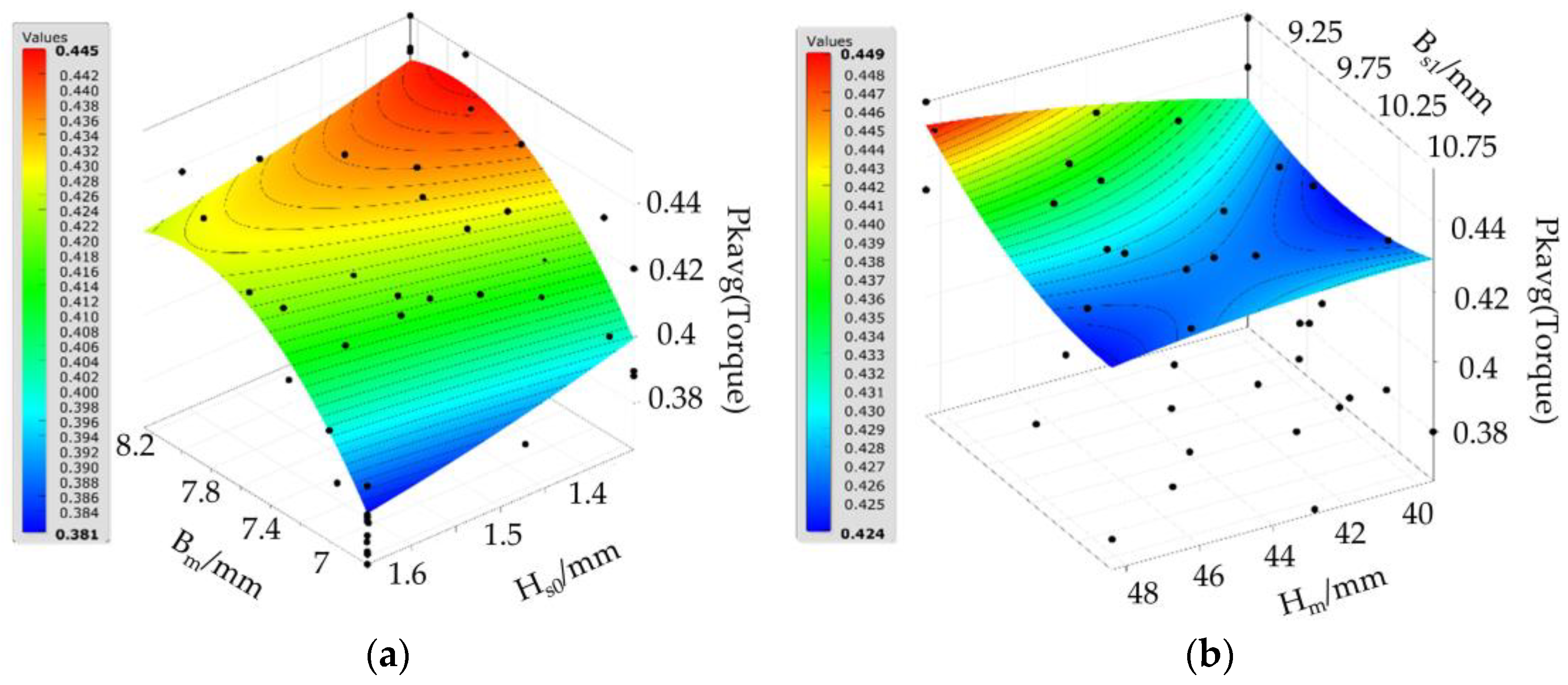
Figure 7 are based on regression analysis using the MFS-MLS method. The 3D response surface of the stator core loss is shown in
Figure 5. The average stator core loss ranges from 630 W to 670 W. As illustrated in
Figure 5a, the average stator core loss increases gradually with both the slot core width
Bs1 and slot height
Hs0, reaching a maximum value of 667 W, with a steep gradient on the response surface. From
Figure 5b, as the permanent magnet thickness
Bm increases and the magnet width
Hm decreases, the average stator core loss also tends to increase, reaching a maximum value of 652.5 W, although the gradient in this region is less steep.
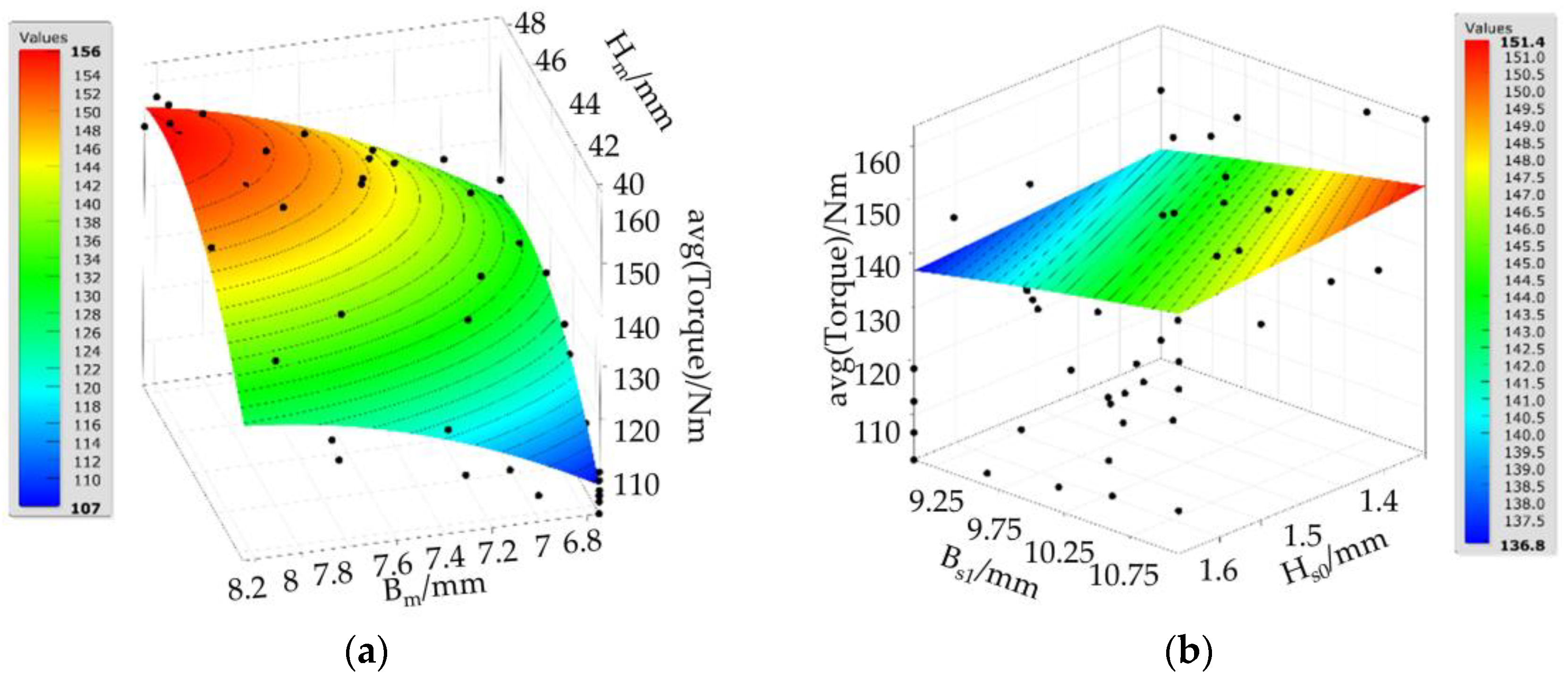
The 3D response surface of the average output torque is depicted in
Figure 6. As shown, increasing both the thickness
Bm and width
Hm of the permanent magnet results in a gradual increase in the average output torque, with a steep response surface gradient. Additionally, the torque increases as the slot core width
Bs1 expands from 9.25 mm to 10.75 mm, while the slot height
Hs0 decreases from 1.6 mm to 1.35 mm.
Figure 7 displays the 3D response surface of the torque ripple. As observed in
Figure 6a, increasing
Bm from 6.8 mm to 8.2 mm and decreasing
Hs0 from 1.6 mm to 1.35 mm causes the torque ripple to increase, with a notable steep gradient. In
Figure 6b, reducing
Bs1 10.75 mm to 9.25 mm and increasing
Hm increases from 40 mm to 48 mm initially decreases the torque ripple, but further increases in Hm lead to a rise in ripple.
Figure 8 illustrates the 3D response surface of the radial electromagnetic force amplitude on the circle. Enlarging both the slot core width
Bs1 from 9.25 mm to 10.75 mm and the magnet width
Hm from 40 mm to 48 mm, as well as increasing the magnet thickness
Bm from 6.8 mm to 8.2 mm and decreasing
Hs0 from 1.6 mm to 1.35 mm, leads to a corresponding increase in the radial electromagnetic force.
As shown in
Table 4, we conducted an empirical comparison using the same DOE samples (
Section 3) to evaluate MFS-MLS against three common techniques.
Table 4 demonstrates that MFS-MLS achieved superior R
2 values for torque-related responses due to its adaptive weighting mechanism. In contrast, Kriging exhibited limitations in handling non-stationary responses, notably the abrupt variations in electromagnetic force at H
m = 46.3 mm. Furthermore, neural networks required a training dataset three times larger than MFS-MLS to attain comparable accuracy, rendering them computationally prohibitive within the 60-iteration MOGA framework.
The structural parameters of the PMSM before and after optimization are summarized in
Table 5. The optimized design parameters are as follows: the width of the permanent magnet
Hm is 46.338 mm, the thickness of the permanent magnet
Bm is 6.914 mm, the width of the slot core
Bs1 is 9.324 mm, and the height of the slot
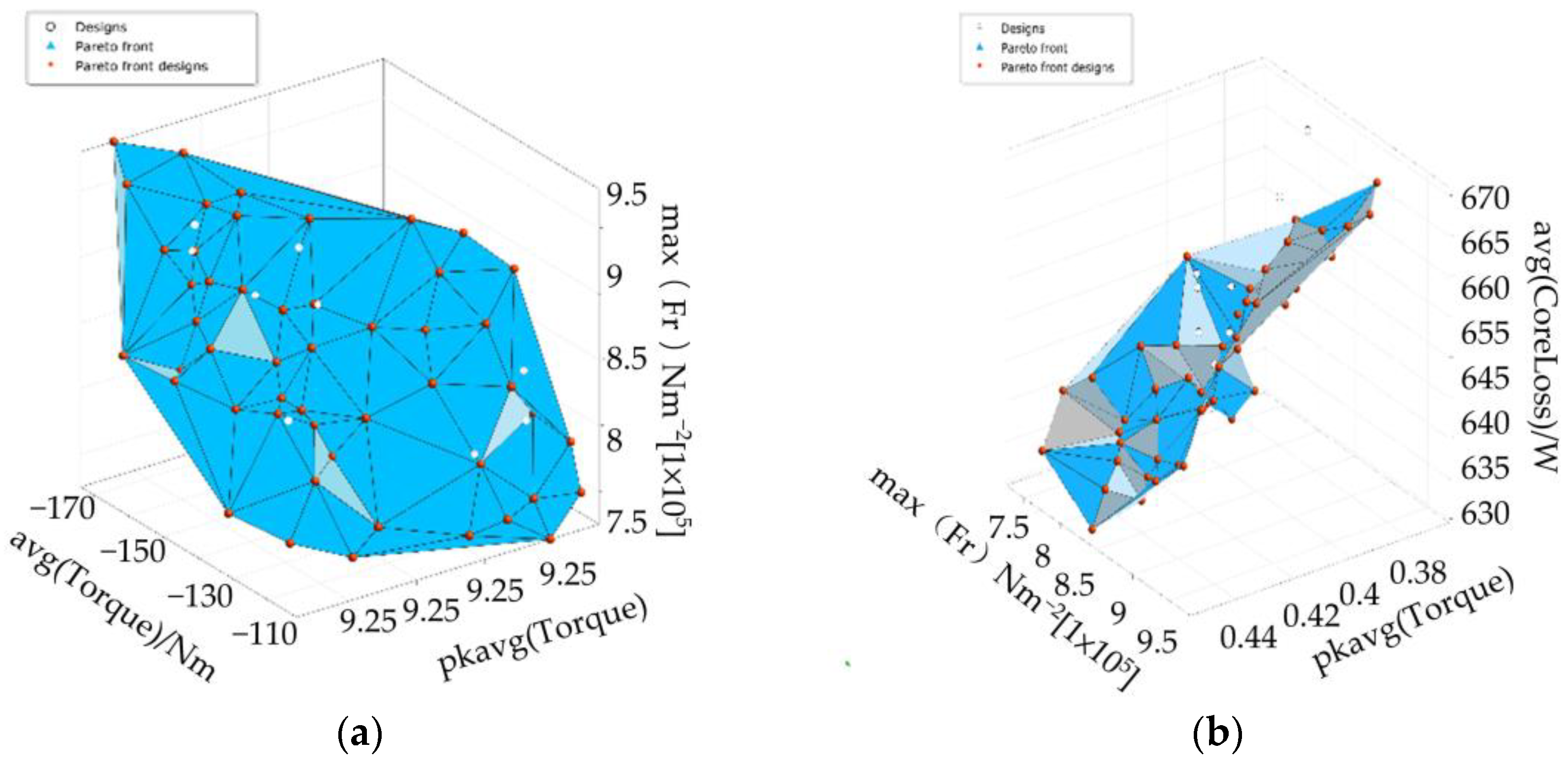
Hs0 is 1.495 mm. The Pareto front of the multi-objective optimization for the PMSM is depicted in
Figure 8. As shown, decreasing the average output torque concurrently reduces both the torque ripple and the radial electromagnetic force. Conversely, increasing the radial electromagnetic force tends to decrease torque ripple but results in higher stator core losses.
Figure 9 presents a comprehensive illustration of the characteristics of the Pareto front, encompassing the following: (1) complete coverage of core loss (ranging from 630 W to 670 W), achievement of 90% of the torque target (spanning from 0.38 N·m to 0.44 N·m), and a comprehensive representation of the force density spectrum (varying between 7.5 N/m
2 and 9.5 × 10
5 N/m
2), with an irregular polyhedral structure that confirms a balanced trade-off among multiple objectives; (2) the formation of a continuous front (depicted by red dots) devoid of discontinuities, juxtaposed with densely distributed design points (indicated by blue triangles). This configuration displays continuous distributions across objectives, uniform spacing of core loss (without clustering), dispersed torque solutions (absence of dense regions), and stepwise intervals for force density (exhibiting balanced spacing). The integrated continuity results in optimal spacing metrics (less than 0.1) and a high hypervolume (HV exceeding 0.85), collectively substantiating the superior quality of solutions for motor optimization design.


 ,
, 


