Flow-Induced Vibration Stability in Pilot-Operated Control Valves with Nonlinear Fluid–Structure Interaction Analysis

Abstract

Control valves in nuclear systems operate under high-pressure differentials generating intense transient fluid forces that induce destructive structural vibrations, risking resonance and the valve stem fracture. In this study, computational fluid dynamics (CFD) was employed to characterize the internal flow dynamics of the valve, supported by experiment validation of the fluid model. To account for nonlinear structural effects such as contact and damping, a coupled fluid–structure interaction approach incorporating nonlinear perturbation analysis was applied to evaluate the dynamic response of the valve core assembly under fluid excitation. The results indicate that flow separation, re-circulation, and vortex shedding within the throttling region are primary contributors to structural vibrations. A comparative analysis of stability coefficients, modal damping ratios, and logarithmic decrements under different valve openings revealed that the valve core assembly remains relatively stable overall. However, critical stability risks were identified in the lower-order modal frequency range at 50% and 70% openings. Notably, at a 70% opening, the first-order modal frequency of the valve core assembly closely aligns with the frequency of fluid excitation, indicating a potential for critical resonance. This research provides important insights for evaluating and enhancing the vibration stability and operational safety of control valves under complex flow conditions.

1. Introduction

As a strategic cornerstone of the national energy structure, nuclear power places utmost importance on safety and reliability. Within nuclear systems, particularly in the reactor’s cooling, heat exchange, and steam circulation circuits, there are complex demands for water flow and pressure regulation. Control valves play a critical role in managing the flow of the coolant and steam—especially in the reactor cooling system—where they precisely regulate coolant flow and pressure to maintain safe reactor temperatures and prevent overheating or equipment failure [1,2,3]. However, under conditions of high-pressure differentials, the narrow flow paths inside control valves can give rise to complex hydrodynamic behavior. The resulting transient, high-energy fluid forces act on the valve core assembly, inducing flow-induced vibrations through dynamic structural response. In severe cases, this may even lead to the resonance and fracture of the valve core components [4,5,6]. The dynamic sensitivity of the valve structure to such fluid excitation is governed by its natural frequency, vibration modes, and damping characteristics.

Extensive research has been conducted on flow-induced vibrations in control valves subjected to fluid excitation forces. F. Chen et al. [7,8,9] combined theoretical analysis and numerical simulation to investigate FIV and noise in fuel control valves used in gas turbines. Their study identified that asymmetric flow at the throttling region causes uneven forces on the valve core, with deflected flow being the primary driver. The use of perforated plates was found effective in correcting this flow asymmetry. Wei A. et al. [10] performed a fluid–structure interaction (FSI) analysis of cryogenic control valves using liquid nitrogen. By employing user-defined functions and dynamic mesh techniques, they simulated the motion of the valve core and revealed the evolution of cavitation flow patterns and their coupling mechanisms with valve core vibrations under cryogenic conditions. Zhang Y. et al. [11] conducted numerical simulations of FIV in nuclear power plant ejectors and established an experimental loop to validate their fluid model. They explored the impact of gas-phase cavitation and pressure fluctuations on structural vibrations, noting that the vibrations exhibited broadband characteristics. Jin H. et al. [12] investigated vibration behavior in multi-stage reverse-flow channels of pressure-reducing control valves using FSI simulations. Their results showed that vortex shedding induced by high-pressure flow through the valve core channel was the dominant excitation mechanism. Phase analysis of valve core vibration intensity further clarified its behavior across different operational stages. Y. Duan. et al. [13] combined simulation and experiments to examine fluid flow around the spindle of a high-pressure valve. By monitoring the frequency of fluid-induced excitation forces and analyzing the influence of the valve opening, they observed a linear decrease in excitation force with an increasing opening, offering insights into identifying high-frequency vibration risks. A. Zeid. et al. [14] conducted three-dimensional FSI simulations on control valves with various recess geometries and openings. The study compared flow characteristics and assessed their impact on vibration and noise, providing design references for low-noise and high-efficiency valve optimization. G. Zhang et al. [15] analyzed cryogenic cavitation-induced vibration in LNG butterfly valves via numerical simulation. By incorporating the thermal effects of cryogenic media into the cavitation model, they studied the dynamic cavitation intensity under different valve openings and the interaction between cavitation and vortex structures. H. Yang. et al. [16] performed a numerical analysis of cavitation-induced vibration in flapper-nozzle servo valves. The study compared the effects of inlet pressure, casing diameter, and gap size on cavitation behavior and proposed the introduction of continuous micro-jets into the main nozzle stream to suppress cavitation. W. Haimin. et al. [17] employed CFD methods to analyze a three-dimensional unsteady flow inside a triple-eccentric butterfly valve. He obtained the Strouhal number of vortex shedding frequency and conducted experimental modal analysis to determine the natural frequency of the valve disk–stem assembly. The results indicated that the structural natural frequency was sufficiently distant from peak steam pressure fluctuation frequencies, thus avoiding resonance or lock-in phenomena. D. Xu et al. [18] used spectral data of transverse lift coefficients induced by vortex shedding as an indicator for valve vortex-induced vibration. By analyzing dominant vibration frequencies and amplitudes, they found that pressure differentials were the main factor influencing vortex-induced vibration. Additionally, a thermal-fluid-structural coupled modal analysis was carried out to assess whether the vortex shedding frequency matched structural modal frequencies, thereby identifying potential resonance risks. Most existing studies on flow-induced vibration (FIV) in control valves focus primarily on the evolution of internal flow fields and the frequency response of fluid excitation forces. However, the structural dynamic behavior of valve components is often analyzed under linear assumptions, without accounting for nonlinear effects such as frictional damping and spring damping arising from contact interactions between internal mechanical components.

To address this gap, the present study conducts CFD simulations to investigate the transient flow field evolution and dominant flow structures within a pilot-operated control valve. Comparative analyses are performed on the frequency characteristics of fluid excitation forces under different valve openings. Furthermore, a nonlinear perturbation-based fluid–structure interaction (FSI) approach is employed to conduct complex modal analysis of the valve core assembly. This study aims to assess the structural stability of the pilot valve under fluid excitation and to provide theoretical insights and practical guidance for the design of more efficient and robust control valves.

2. Flow Analysis of Pilot-Operated Regulating Valve

2.1. Structure and Working Principle of Control Valve

The pilot-operated control valve, as shown in Figure 1, primarily comprises a valve body, valve core, valve seat, and sleeve, with Figure 2 illustrating the sleeve’s 2D structure diagram. Fluid enters through the inlet on the left, passes through the throttling section formed by the valve core, and exits to the right through the sleeve. The actuator regulates the valve core position, thereby adjusting the valve opening and controlling the flow area within the valve body. This enables the precise regulation of both flow rate and pressure. The operating conditions of the pilot-operated control valve and the physical properties of its key components are listed in

Table 1. Operating conditions of the pilot-operated control valve.

Name	Nominal Diameter	Operating Temperature	Operating Pressure	Valve Stroke	Working Medium
Parameter	DN50	25 °C	1 MPa	22 mm	water

and

Table 2. Material parameters of the pilot-operated control valve parts.

Parts	Material	Destiny ρ/(kg/m3)	Poisson Ratio	Elastic Modulus E (GPa)
Valve core, valve stem	304	7930	0.29	200
Valve body	CF8	7850	0.29	193
Valve bonnet	F304	7930	0.29	193

, respectively.

2.2. Flow Analysis

2.2.1. Turbulence Model

The fluid in the regulating valve will generate strong swirling flow during the flow process, using standard k-ɛ. The turbulence model can generate simulation distortion, so this chapter uses RNG k-ɛ. The two-equation turbulence model is used for the transient simulation of the internal flow field of the regulating valve. This model not only corrects the turbulent viscosity, but also considers the rotation situation and time-averaged strain rate in the fluid flow, improving simulation accuracy. In addition, the source term in the model is not only related to the fluid flow situation, but also a function of spatial coordinates, which can better handle flows with high strain rates and large streamline curvature. The basic control equation of the RNG k-ɛ model is shown in the following equation.

$${\displaystyle \frac{\mathsf{\partial }k}{\mathsf{\partial }t}}+{\displaystyle \frac{\mathsf{\partial }(k{u}_i)}{\mathsf{\partial }{x}_i}}={\displaystyle \frac{1}{\rho }}{\displaystyle \frac{\mathsf{\partial }}{\mathsf{\partial }{x}_j}}\left[a_k(\mu +\rho C_{\mu }{\displaystyle \frac{k^2}{\epsilon }}){\displaystyle \frac{\mathsf{\partial }k}{\mathsf{\partial }{x}_j}}\right]+{\displaystyle \frac{G_k}{\rho }}+\epsilon ,$$

(1)

$${\displaystyle \frac{\mathsf{\partial }\epsilon }{\mathsf{\partial }t}}+{\displaystyle \frac{\mathsf{\partial }(\epsilon u_i)}{\mathsf{\partial }{x}_i}}={\displaystyle \frac{1}{\rho }}{\displaystyle \frac{\mathsf{\partial }}{\mathsf{\partial }{x}_j}}\left[a_{\epsilon }(\mu +\rho C_{\mu }{\displaystyle \frac{k^2}{\epsilon }}){\displaystyle \frac{\mathsf{\partial }\epsilon }{\mathsf{\partial }{x}_j}}\right]+{\displaystyle \frac{1}{\rho }}{\displaystyle \frac{\epsilon C_{i\epsilon }^{*}{G}_k}{k}}-{\displaystyle \frac{{\epsilon }^2{C}_{2\epsilon }}{k}},$$

(2)

In the equation, $G_{\mathrm{k}}$ is the turbulent kinetic energy generation term caused by the average velocity gradient, and its equation is

$$G_{\mathrm{k}}={\mu }_{\mathrm{t}}\left\{\begin{array}{l}2\left[{\left({\displaystyle \frac{\mathsf{\partial }u}{\mathsf{\partial }x}}\right)}^2+{\left({\displaystyle \frac{\mathsf{\partial }v}{\mathsf{\partial }y}}\right)}^2+{\left({\displaystyle \frac{\mathsf{\partial }w}{\mathsf{\partial }z}}\right)}^2\right]+\\ {\left({\displaystyle \frac{\mathsf{\partial }u}{\mathsf{\partial }y}}+{\displaystyle \frac{\mathsf{\partial }v}{\mathsf{\partial }x}}\right)}^2+{\left({\displaystyle \frac{\mathsf{\partial }u}{\mathsf{\partial }z}}+{\displaystyle \frac{\mathsf{\partial }w}{\mathsf{\partial }x}}\right)}^2+{\left({\displaystyle \frac{\mathsf{\partial }v}{\mathsf{\partial }z}}+{\displaystyle \frac{\mathsf{\partial }w}{\mathsf{\partial }y}}\right)}^2\end{array}\right\},$$

(3)

Among them $k={\displaystyle \frac{\overline{u_i^{\prime }{u}_j^{\prime }}}{2}}={\displaystyle \frac{1}{2}}(\overline{u^{\prime 2}}+\overline{v^{\prime 2}}+\overline{w^{\prime 2}})$, $\epsilon ={\displaystyle \frac{\mu }{\rho }}({\displaystyle \frac{\mathsf{\partial }{u}_i^{\prime }}{\mathsf{\partial }{x}_k}})({\displaystyle \frac{\mathsf{\partial }{u}_j^{\prime }}{\mathsf{\partial }{x}_k}});$

$C_{1\epsilon }^{*}=1.42-{\displaystyle \frac{\eta (1-\eta /4.377)}{1+0.012{\eta }^3}}$;

$\eta ={(2E_{ij}\cdot E_{ij})}^{1/2}{\displaystyle \frac{k}{\epsilon }}$, $E_{ij}={\displaystyle \frac{1}{2}}({\displaystyle \frac{\mathsf{\partial }{u}_i}{\mathsf{\partial }{x}_j}}+{\displaystyle \frac{\mathsf{\partial }{u}_j}{\mathsf{\partial }{x}_i}})$;

$C_{\mu }=0.0845, {\alpha }_k={\alpha }_{\epsilon }=1.39, C_{2\epsilon }=1.68$.

The inlet is set to the pressure inlet boundary condition, and the outlet is set to the pressure outlet boundary condition. The wall function processes the near-wall area. The above control equations are discretized in space. The coupling of velocity and pressure is realized by the couple algorithm. The discretization method of the pressure term adopts the Standard format, and the other terms adopt the second-order upwind format. During calculation, a steady-state calculation is performed first, and the result is used as the initial value of the unsteady calculation to ensure the stability and convergence speed of the calculation. In order to ensure that the flow characteristics can be fully observed on the microscopic time scale, and to save computing resources as much as possible, the simulation time step here is set to ∆t = 0.1 μs.

2.2.2. Flow Domain Geometry and Computational Mesh

Geometric models of the pilot-operated control valve were established for various valve openings. To ensure fully developed flow conditions, straight pipe extensions measuring five and ten times the nominal diameter were added upstream and downstream of the valve, respectively. To enhance computational efficiency and improve convergence without compromising accuracy, minor geometric features such as filets and chamfers—considered to have minimal influence on fluid behavior—were appropriately simplified. Based on the simplified geometry, the internal flow domain was extracted through reverse modeling to generate the computational flow passage model. The resulting flow domain of the pilot-type contoured sleeve control valve is illustrated in Figure 3.

The Fluent Mosaic™ meshing technology was employed to discretize the flow domain of the pilot-operated control valve. In the regular regions and areas distant from geometric boundaries—such as the upstream and downstream pipelines—structured hexahedral meshes were applied. For complex geometries within the valve chamber, such as the flow passages, polyhedral meshes were generated to accurately capture intricate flow behavior. In critical regions like the throttling orifice, the minimum mesh size was refined to 0.01 mm to ensure sufficient resolution for capturing high-speed flow features while maintaining mesh quality. To ensure a smooth mesh transition, a combination of tetrahedral and pyramidal elements was used in intermediate regions. Local mesh refinement was applied in areas requiring high-resolution flow capture, such as the throttling gaps, sharp corners, and narrow passages within the valve. Boundary layer meshes were generated to resolve near-wall flow features, which are essential for turbulence models based on wall functions. For these models, the ideal y⁺ value range lies between 30 and 100. The thickness of the first boundary layer, Δy₁, can be estimated either through preliminary calculations or empirical formulas. Assuming a target y⁺ of 30, a friction velocity (u_τ) of 0.1 m/s, and a dynamic viscosity (μ) of water as 1.002 × 10⁻³ Pa·s, the estimated Δy₁ is approximately 0.301 mm. Seven layers were used in the boundary layer mesh, with a thickness growth ratio of 1.2 between adjacent layers to ensure the smooth transition and accurate resolution of the boundary layer. To maintain mesh quality and numerical stability, boundary layer elements were designed to be as orthogonal as possible, with a skewness less than 0.85. All simulations were performed using ANSYS Fluent 2022 R1. The convergence criteria were set so that the residuals for continuity and momentum equations were reduced below 1 × 10⁻⁵, and key physical quantities such as pressure drop and velocity reached stable values over successive iterations. Using the Fluent Mosaic™ meshing strategy, four mesh configurations for the control valve flow domain were generated, as summarized in

Table 3. Mesh independence verification.

Mesh	Nodes Number	Elements Number	Flow Rate (kg/h)
1	695,141	3,413,174	5173.2
2	843,521	4,300,733	5778.5
3	10,733,368	5,313,572	5892.4
4	13,406,521	6,503,801	5894.7
5	13,406,521	6,503,801	5894.7

and illustrated in Figure 4. A mesh independence study was conducted, and the final mesh model adopted for the flow domain is shown in Figure 5.

A comparative analysis was conducted using five mesh configurations with varying numbers of cells. For each configuration, the inlet pressure was recorded throughout the simulation, as shown in Figure 5. The results indicate that all mesh configurations exhibited a similar trend: the inlet pressure gradually increased with the number of iterations. Meshes with fewer cells converged more quickly but resulted in slightly different final pressure values. To ensure the accuracy of the comparison, the average inlet pressure over the final 500 iterations was used for evaluation. The analysis revealed a notable increase in average inlet pressure as the mesh size increased from 3.4 million to 5.3 million cells. However, when the mesh size was further increased to 6.5 million cells, the pressure slightly decreased. A detailed examination of the pressure variation shows the following: compared to the 3.4 million-cell mesh, the 4.3 million-cell mesh yielded a 5.1% increase in average inlet pressure. Increasing the mesh to 5.3 million cells led to a further 1.9% rise. However, the increase from 5.3 million to 6.5 million cells resulted in only a 0.9% change, indicating diminishing returns in pressure accuracy. Based on these findings, the mesh configuration with 5.3 million cells was selected for subsequent analysis.

2.2.3. Experimental Procedure

A flow testing system was designed and constructed to evaluate the performance of a control valve and its associated piping under various operating conditions, as illustrated in the schematic diagram shown in Figure 6. The experimental setup is depicted in Figure 7. The system was developed to measure the flow rate through the control valve at specific valve openings (10%, 30%, 50%, 70%, and 100%) to assess its flow conditions. The test setup included a centrifugal pump, stainless steel piping (DN50), a throttling valve downstream of the control valve, and an EMERSON8750W (Emerson Electric Co., St. Louis, MO, USA) series electromagnetic flowmeter positioned upstream to continuously monitor and record flow rate data in real time.

During testing, the upstream pressure of the valve was maintained at 1 MPa, while the downstream side was exposed to atmospheric pressure. The working fluid was water at an ambient temperature of 20 ± 2 °C, ensuring consistent fluid properties across all tests. The EMERSON8750W flowmeter, with a nominal diameter of DN50 and an accuracy class of 0.5, was selected for its high precision in turbulent flow regimes. The flowmeter was calibrated before testing using a certified reference standard to ensure measurement accuracy within ±0.5% of the full scale.

2.2.4. Validation of Numerical Model

Validation of the current numerical model was performed to ensure the accuracy of the simulated results. Figure 8 shows a comparison between simulations by three different turbulence models and the experimental results of the mass flow rate of different openings. And the three turbulence models include Realizable k-ε, RNG k-ε, and SST k-ω. It can be seen that three turbulence models are in good agreement with the experimental data and the results obtained by the RNG k-ε model is closer to the experimental data. The errors between experimental data and numerical simulations are less than 10%. The greater the opening, the higher the calculation accuracy. Hence, considering its advantages, the RNG k-ε model was employed in this study and the validation of the current numerical model was performed.

2.3. Flow Analysis Results and Discussion

A comprehensive analysis of pressure contours, velocity streamlines, and turbulent kinetic energy (TKE) distributions within the pilot-operated control valve was conducted to identify the key factors contributing to flow-induced instabilities. Figure 9 illustrates the pressure distribution inside the valve at different time steps. As shown, when fluid passes through the throttling region, a pressure drop can occur due to increased flow velocity or flow separation as the fluid is compressed. Notable pressure fluctuations are observed at the main valve inlet and in the downstream valve chamber. These variations are primarily driven by the alternating behavior of valve modulation and dynamic flow conditions. The pressure distribution near the main valve spool inlet exhibits an asymmetric and non-uniform pattern, with localized high- and low-pressure zones. These features are closely associated with turbulence, recirculation, and flow separation phenomena within the valve.

Figure 10 presents the flow patterns and turbulence characteristics within the control valve. The streamline distributions reveal that as the fluid passes through the throttling components, its flow behavior is significantly influenced by the valve’s geometry. In particular, regions near the throttling orifice and valve seat exhibit clear signs of flow separation, recirculation, and vortex formation. These complex flow features indicate a high degree of flow instability and the onset of turbulence, especially under high Reynolds number conditions, which can lead to drastic changes in flow regime. The presence of recirculation zones and vortices may induce vibrations in the valve’s moving components and negatively affect the efficiency and stability of flow regulation.

Figure 11 shows the distribution of turbulent kinetic energy (TKE) within the control valve. The results indicate that TKE is primarily concentrated in the local throttling regions of the valve, which are typically associated with flow separation, recirculation, and vortex formation. These high-TKE regions reflect significant velocity fluctuations and strong flow instability. The distribution of TKE is heavily influenced by the geometry of the throttling zones, leading to complex flow patterns in these areas. This effect becomes more pronounced at smaller valve openings, where higher fluid velocities intensify the turbulence. As the fluid navigates through multiple sharp turns within the valve, the TKE increases significantly, potentially resulting in severe flow phenomena such as vortex shedding and flow separation.

Under a constant pressure drop condition (ΔP = 1 MPa), the flow-induced excitation forces acting on the spool of the pilot-operated control valve were analyzed using time- and frequency-domain methods across four representative valve openings (10%, 30%, 50%, and 70%). As shown in Figure 12, at a 30% valve opening, the dynamic load from the incompressible fluid exhibited pronounced nonlinear behavior, with the axial excitation force reaching a peak amplitude of 6000 N—over a 500% increase compared to other operating conditions. Frequency-domain analysis revealed that, at this opening, the high-energy excitation forces were concentrated within the 100–300 Hz range, with the dominant excitation frequency observed at 157 Hz. In contrast, for the 50% and 70% openings, the time-domain excitation force amplitudes remained below 1000 N, indicating more stable flow conditions. The 50% opening showed a dual-peak energy spectrum centered at a base frequency of 200 Hz and its third harmonic at 600 Hz. The 70% opening exhibited a broadband excitation pattern, with energy distributed up to 1000 Hz and containing multiple higher-order harmonic components. These findings indicate that, under a 1 MPa pressure drop, the primary energy of flow-induced excitation forces is concentrated below 500 Hz across all valve openings. However, the 30% opening condition demonstrates critical-level energy density due to intensified turbulent kinetic energy dissipation caused by abrupt flow channel changes.

3. Nonlinear Modal Analysis

3.1. Principle of Fluid–Structure Coupling Modal Analysis

To analyze the inherent modal matrix of a multi-degree-of-freedom fluid–structure interaction system in a control valve, a coordinate transformation is performed, transforming the system into a series of single-degree-of-freedom systems described by principal coordinates. These systems are then solved individually, and the solution to the multi-degree-of-freedom system is obtained using the principle of superposition. When solving for the control valve core-motion component structure’s inherent modes, the influence of the surrounding fluid needs to be considered. The governing equations for the structure–fluid system of the control valve core-motion component can be written as

$$M_s\ddot{r}+C_s\dot{r}+K_{s}r=B^{T}p-f_0,$$

(4)

$$E\ddot{p}+A\dot{p}+Hp=-\rho B\ddot{r}-q_0,$$

(5)

For incompressible fluids, A→0, and when the free surface effect is neglected, E→0. If, in this context, the input excitation vector is also ignored, the undamped free vibration equations of the FSI system (C_s = 0, f₀ = 0) can be represented as

$$\left[\begin{array}{c}{H}_{rr} H_{rh}\\ H_{hr} H_{hh}\end{array}\right]\left[\begin{array}{c}{p}_r\\ P_h\end{array}\right]=\left[\begin{array}{c}0\\ -\rho B\ddot{r}\end{array}\right],$$

(6)

$$M_0\ddot{r}+K_{n}r=B^{T}p,$$

(7)

In these equations, p_h represents the node pressure vector at the fluid–structure interface of the control valve core-motion component structure, while p_r represents the pressure vector at the remaining nodes. The matrices H_rr, H_rh, H_hr, and H_hh are submatrices of H corresponding to P_h and P_r. By combining the first and second rows of Equation (6), we obtain

$$p_h=-\rho H_h^{-1}B\ddot{r},$$

(8)

In the motion equation of the control valve core-motion component structure system given by Equation (7), the right-hand term contains the node pressure vector p, which can be reduced to its subset p_h, the node pressure vector at the fluid–structure interface. Substituting Equation (8) into Equation (7) yields

$$(M_s+M_a)\ddot{r}+K_{a}r=0,$$

(9)

Here, M_a represents the mass matrix of the control valve core-motion component structure, $M_a=\rho B^T{H}_h^{-1}B$, Ms is the added mass matrix, and Ka is the structure’s stiffness matrix. As observed, when considering fluid–structure coupling, the inertial terms in the undamped free vibration equation are influenced by the added mass effect.

Matrix Ma contains H_h⁻¹, thus making Ma a full matrix. The dimension of matrix Ma is generally smaller than that of M_s, with the bandwidth primarily determined by the size of M_a if the interface is large.

The characteristic equation of Equation (9) is given by |K_a−λ_n²(M_s+ M_a)| = 0, where λ_n represents the damped mode frequency of the fluid–structure coupled system of the valve core-motion component of the regulating valve. From this, the natural frequencies and damped mode vectors φ of the fluid–structure system of the valve core-motion component can be determined.

Let

$$\phi =\left[\begin{array}{c}{\phi }_0\\ {\phi }_1\end{array}\right],r=\left[\begin{array}{c}{r}_0\\ r_1\end{array}\right]\begin{array}{cc}& \end{array}r=\phi .q,$$

(10)

where 0 refers to “dry” node codes, 1 refers to “wet” node codes, r is the displacement vector at the fluid–structure interface, and q is the generalized coordinate vector. Equation (9) can then be simplified to

$$\left[\begin{array}{cc}{M}_{00}& M_{01}\\ M_{10}& M_{11}+M_a\end{array}\right]\left[\begin{array}{c}{\ddot{r}}_0\\ {\ddot{r}}_1\end{array}\right]+\left[\begin{array}{cc}{K}_{00}& K_{01}\\ K_{10}& K_{11}\end{array}\right]\left[\begin{array}{c}{r}_0\\ r_1\end{array}\right]=0,$$

(11)

By substituting Equation (10) into Equation (11) for diagonalization, we obtain:

$${\left[\begin{array}{c}{\phi }_0\\ {\phi }_1\end{array}\right]}^T\left[\begin{array}{cc}{M}_{00}& M_{01}\\ M_{10}& M_{11}+M_a\end{array}\right]\left[\begin{array}{c}{\phi }_0\\ {\phi }_1\end{array}\right].\ddot{q}+{\left[\begin{array}{c}{\phi }_0\\ {\phi }_1\end{array}\right]}^T\left[\begin{array}{cc}{K}_{00}& K_{01}\\ K_{10}& K_{11}\end{array}\right]\left[\begin{array}{c}{\phi }_0\\ {\phi }_1\end{array}\right].q=0,$$

(12)

where ${\left[\begin{array}{c}{\phi }_0\\ {\phi }_1\end{array}\right]}^T\left[\begin{array}{cc}{M}_{00}& M_{01}\\ M_{10}& M_{11}+M_a\end{array}\right]\left[\begin{array}{c}{\phi }_0\\ {\phi }_1\end{array}\right]=I$,${\left[\begin{array}{c}{\phi }_0\\ {\phi }_1\end{array}\right]}^T\left[\begin{array}{cc}{K}_{00}& K_{01}\\ K_{10}& K_{11}\end{array}\right]\left[\begin{array}{c}{\phi }_0\\ {\phi }_1\end{array}\right]={\Lambda }_0^{\prime }$

${\mathrm{\Lambda }}_0^{\prime }=\left[\begin{array}{cccc}{\lambda }_{01}^2& & & \\ & {\lambda }_{02}^2& & \\ & & & \\ & & & {\lambda }_{0n}^2\end{array}\right]$

In the formula, $\mathit{\Lambda }{\prime }_0$ is the wet mode natural frequency of the valve core-motion component.

3.2. Boundary Conditions

To accurately assess the structural dynamic characteristics of the control valve under operational conditions, the effects of fluid excitation forces and nonlinear contact interactions between internal components were incorporated. The fluid pressure field was initially computed using ANSYS Fluent 2022 R1. The resulting pressure distribution was then mapped and applied as a boundary load to the structural model analyzed in ANSYS Mechanical, establishing a fluid–structure coupling. To address the limitations of traditional real-mode analysis—particularly the neglect of asymmetric damping effects—a nonlinear perturbation approach was adopted for the prestressed FSI modal analysis of the control valve, reflecting the nonlinear behavior due to large deformations, frictional contacts, and dynamic interactions.

During the FSI prestress analysis, realistic contact relationships among structural components were meticulously defined, including frictional contact between the valve spool and sleeve, which introduces nonlinear force-displacement relationships varying with contact state and relative motion, as well as the nonlinear damping effects of springs within the pilot valve spool assembly. Using the perturb command, a small-displacement analysis was conducted around the system’s equilibrium state. To account for matrix asymmetry and the influence of large deformations on the stiffness matrix, a non-symmetric Newton–Raphson solver was employed, with both large deformation and restart options enabled, further addressing the nonlinear stiffness and damping behavior under prestress conditions. The QR damping algorithm was also activated to enhance the stability of eigenvalue computations for the asymmetric system matrix. Given the structural complexity and large matrix size of the control valve model, the Lanczos method was utilized to compute the complex eigenmodes in the FSI prestressed modal analysis. The relevant APDL code used for this analysis is as follows:

ANTYPE, STATIC, RESTART, PERTURB

PERTURB, MODAL

SOLVE, ELFORM

QRDOPT, ON

MODOPT, UNSYM, 24

MXPAND

SOLVE

3.3. Structural Geometry and Computational Mesh

The geometric model of the spool-stem assembly of the pilot-operated control valve, which retains the core structural features such as the valve spool, stem, and sleeve, is shown in Figure 13. A mixed mesh strategy dominated by hexahedral elements was employed, using a Body-Fitted Cartesian meshing approach for the spool-stem assembly. This method combines global structured Cartesian meshing with local geometry-adaptive cutting, enabling high-fidelity representation of curved sleeve boundaries while preserving the computational advantages of structured grids. Local adaptive mesh refinement was applied in regions with geometric discontinuities—such as damping holes—to effectively reduce stress inaccuracies typically caused by staircase-like boundaries. Automatic topology optimization was used to mitigate cell distortion issues common in unstructured meshes. Additionally, a background grid–cut cell coupling algorithm was implemented to maintain the stiffness matrix stability, thereby enhancing numerical convergence without compromising computational efficiency or accuracy.

To verify mesh independence, six levels of progressively refined meshes were generated for modal analysis. The first six natural frequencies (wet modes) were extracted, and the relative deviations between adjacent mesh levels were quantified. Figure 14 presents the modal frequency comparison across different mesh densities. The results show that within the range of 173,000 to 185,000 elements, modal frequencies increased with mesh density, with deviations as high as 9%. Beyond 193,000 elements, the frequencies began to stabilize, and the deviation reduced to approximately 0.5%. Based on this analysis, a final mesh configuration with 193,607 elements was selected. The corresponding mesh model is shown in Figure 13.

3.4. Results and Discussion

Modal participation factors were calculated based on the modal analysis results of the control valve to determine the effective modes through modal truncation. For the i-th mode, the modal participation factor was computed using the following equation:

$${\mathit{\Gamma }}_i={\displaystyle \frac{{\mathit{\varphi }}_i^T\cdot \mathit{F}}{{\mathit{\omega }}_i^2\cdot {\mathit{\varphi }}_i^T\cdot \mathit{m}\cdot {\mathit{\varphi }}_i}},$$

(13)

where φ_i is the mode shape vector of the i-th mode, F is the external force vector applied to the structure, ${\omega }_i^2$ is the natural frequency of the i-th mode, m is the mass matrix of the structure, and φ_i^T is the transpose of the mode shape vector. The modal participation factors for each direction were calculated and are shown in

Table 4. Modal Participation Factor.

Direction	Modal Participation Factor
X	0.892
Y	0.899
Z	0.875
ROTX	0.937
ROTY	0.924
ROTZ	0.940

.

The computed modal participation factors in the X, Y, and Z translational directions were all between 0.8 and 0.9, while those in the X, Y, and Z rotational directions exceeded 0.9. These values satisfy the commonly accepted threshold for significant modal participation (≥0.8), confirming the reliability of the modal analysis. As a result, the first twelve mode shapes were selected for further analysis.

3.4.1. Modal Frequency and Modal Shape

Figure 15 illustrates the first twelve mode shapes of the valve stem–spool assembly, covering a frequency range from low to mid-high frequencies. The first mode exhibits an overall longitudinal extension and contraction vibration of the assembly, with the maximum displacement occurring at the connection between the valve stem and spool, gradually decreasing toward the constrained boundaries. This mode reflects the fundamental axial stiffness characteristics of the structure. The 2nd mode is dominated by the lateral vibration of the spool, showing pronounced transverse deformation of the spool while the valve stem remains largely undeformed. The 3rd and 5th modes feature the valve stem undergoing S-shaped coupled bending vibrations, with two opposite bending nodes forming spatial S-shaped waveforms; the spool deformation is minimal in these modes. The 4th, 6th, 10th, and 11th modes exhibit torsional vibrations of the valve stem, characterized by two opposite torsion points in the midsection of the stem, indicating torque transmission under asymmetric support conditions. The 7th mode shows the lateral vibration localized in the pilot valve spool. The 8th and 9th modes display segmented coupled vibrations with multiple wave peaks, representing higher-order bending harmonics. The twelfth mode reveals localized high-frequency vibrations at the edges of the pilot valve spool (indicated by yellow-green spots), which may be related to fluid excitation effects.

For the multi-degree-of-freedom damping system considering the spring damping within the valve spool assembly and the nonlinear contact damping between components, the damped modal frequency is expressed as

$$f_{di}=f_{ni}\sqrt{1-{\varsigma }_i^2},$$

(14)

where f_di is the damped frequency of the i-th mode (Hz), f_ni is the undamped natural frequency of the i-th mode (Hz), and ζ_i is the modal damping ratio of the i-th mode.

Using fluid–structure interaction complex modal analysis, the damped frequencies of the first twelve modes of the valve spool assembly were obtained under various valve openings. These results were compared against the undamped real modal frequencies calculated without considering nonlinear contact behaviors and structural damping between spool components. Figure 16 presents the comparison of the first twelve real and complex modal frequencies of the valve spool assembly across different valve openings.

As shown in Figure 16, at valve openings of 10% and 30%, the first two modal frequencies of the valve spool assembly are relatively low, with the first mode frequencies measured at 788.75 Hz and 1183 Hz, respectively. Modal frequencies increase progressively with mode order, exceeding 5000 Hz for higher modes. At 50% and 70% openings, the first four modal frequencies remain relatively low, with the first modal frequencies at 559.57 Hz and 1214.2 Hz, respectively. The trend of higher-order modal frequencies at these openings is consistent with that observed at 10% and 30%. Notably, the high-order damped modal frequencies exhibit minimal variation across different valve openings.

By calculating the relative shift between the complex modal frequencies and the real modal frequencies, it is evident that the complex modal frequencies are slightly lower due to the damping effects introduced by nonlinear contact interactions among spool components and the spring damping. The maximum relative frequency shifts at 10%, 30%, 50%, and 70% valve openings are 4.89%, 2.7%, 1.42%, and 0.46%, respectively. Overall, the complex modal frequency shifts remain modest, all within 5%.

3.4.2. Stability Coefficients

To evaluate the stability of the multi-degree-of-freedom damping system considering both spring damping within the valve spool assembly and nonlinear contact damping between components, the modal stability coefficients of the valve spool system were calculated. For the structure dynamic control Equation (9), assuming its solution form as $\psi e^{{\lambda }_{i}t}$, substitution into Equation (9) yields

$$\left({\lambda }_i^2\left[M\right]+\left[K\right]\right)\left\{\Psi \right\}=\left[D({\lambda }_i)\right]\left\{\Psi \right\}=\left\{0\right\}$$

(15)

The necessary and sufficient condition for the existence of a non-zero solution in Equation (15) is $\left|\left[D({\lambda }_i)\right]\right|=0$

This results in a pair of conjugate roots ${\lambda }_i={\sigma }_i\pm j{f}_d$.

For complex modal analysis, based on the eigenvalue expression, the system’s stability is determined by the real part of the eigenvalues, denoted as σ_i. When the real part σ is negative, the system is stable, when σ_i = 0, the system is marginally stable, and when σ_i is positive, the system is unstable. To assess the stability of the multi-degree-of-freedom damping system that accounts for spring damping within the valve spool assembly and nonlinear contact damping between components, the modal stability coefficients of the valve spool system were calculated. As illustrated in Figure 17, the modal stability coefficient is typically related to the location of the system poles.

As shown in Figure 17, the modal stability coefficients of the multi-degree-of-freedom damping system for the control valve spool assembly are negative across both low and high-order modes, indicating that the system is generally stable. At valve openings of 10% and 30%, the stability coefficients for the 1st, 2nd, and 7th modes approach zero, while at 50% and 70% openings, the stability coefficients of the 1st through 4th modes are also close to zero. This suggests that the system is prone to marginal stability or even potential instability under these modal frequencies. Furthermore, the stability coefficient exhibits a negative correlation with modal order, indicating that the system tends to be more stable and secure under high-frequency excitations.

3.4.3. Modal Damping Ratios and Logarithmic Decrement

To investigate the damping effect of the spring within the control valve spool assembly, as well as the damping induced by nonlinear contact interactions between components, the system’s vibration attenuation capability is evaluated through the analysis of the modal damping ratio. The modal damping ratio ζ is defined as

$$\zeta =c/c_c,$$

(16)

where c is the actual damping coefficient, and c_c is the critical damping coefficient.

Furthermore, the effect of damping on vibration attenuation is quantified using the logarithmic decrement δ_i, which is calculated based on the natural logarithm of the ratio of adjacent vibration amplitudes. The parameter δ_i is based on modal decomposition, where the free decay response of each individual mode is separately fitted

$${\delta }_i=\ln (A_i(t+n{T}_i)/A_i(t))/n$$

(17)

where A_i(t) and A_i(t + nT_i) represent the vibration amplitudes of the i-th mode separated by n periods. This approach enables a quantitative assessment of the system’s damping performance and stability characteristics.

As shown in Figure 18, the modal damping ratios of the multi-degree-of-freedom spool assembly damping system in the control valve are all greater than zero but much less than one across both low- and high-order modes, indicating an underdamped state. Under the action of fluid-induced excitation forces, the system exhibits gradually decaying vibrations, suggesting that the spool assembly system remains relatively stable.

At valve openings of 10% and 30%, the modal damping ratios for the first and seventh modes are nearly zero. Similarly, at 50% opening, the first and fifth modes, and at 70% opening, the third and seventh modes exhibit damping ratios close to zero. This indicates that the system approaches critical stability at these modal frequencies, where its ability to dissipate energy is significantly compromised, making it highly susceptible to sustained vibrations triggered by minor disturbances or continuous fluid excitation. Modal shape analysis reveals that these low-damping modes are typically associated with localized dynamic amplification in specific regions of the valve core assembly, particularly near the transition area between the valve stem and the valve core. These regions are prone to high-cycle fatigue, localized resonance, or contact instability during prolonged operation.

The distribution of modal damping ratios across different modal orders and valve openings is relatively concentrated and generally less than 0.05. Notably, at 10% and 30% openings, the 10th mode, and at 50% and 70% openings, the 12th mode, exhibit significantly higher damping ratios compared to other modes. This demonstrates that the structure is more stable and secure at these modal frequencies.

As shown in Figure 19, the trend of logarithmic decrement for the damping system aligns closely with that of the modal damping ratios. At 10% and 30% openings, the 10th mode, and at 50% and 70% openings, the 12th mode, display markedly higher logarithmic decrements than other modal orders. This indicates that stronger damping effects correspond to faster vibration attenuation.

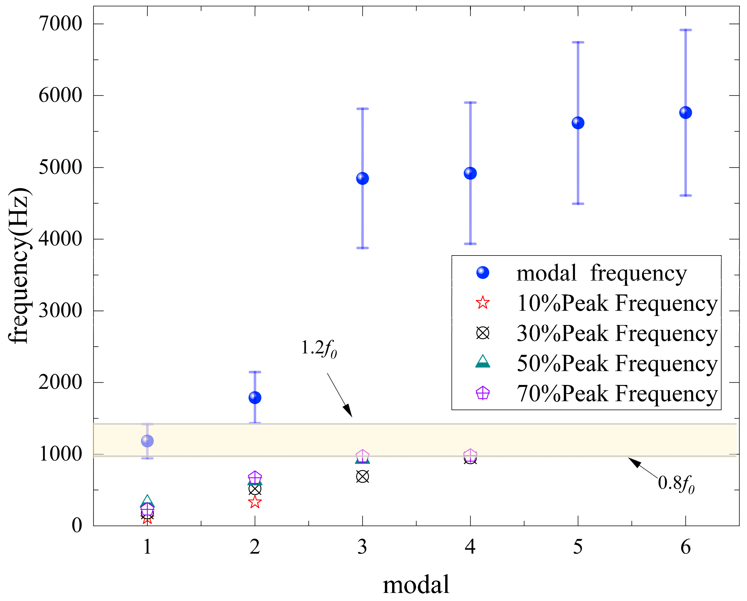
3.4.4. Comparison of Modal and Fluid Excitation Force Frequency

Figure 20 compares the dominant peak frequencies of fluid excitation forces and the complex modal frequencies of the pilot-operated control valve under typical valve openings. As shown, the first six complex modal frequencies of the valve core-stem assembly are all above 1000 Hz, with the first mode at 1183 Hz. In engineering practice, the frequency range between 0.8 and 1.2 times the excitation frequency is typically defined as the resonance zone.

At a 10% valve opening, the dominant excitation frequency is 329 Hz, which differs from the first modal frequency by approximately 72%, indicating low resonance risk. As the valve opening increases, the excitation spectrum becomes broader and the peak frequency increases. At a 70% opening, the peak excitation frequency rises to 959 Hz, which falls within the 0.8–1.2 range of the first modal frequency.

Combining this with the analysis of modal stability factors, modal damping ratios, and logarithmic decrement, it is evident that the valve core-stem assembly is prone to near-critical stability behavior around its first complex modal frequency of 1183 Hz. Therefore, under 50% and 70% openings, the excitation frequency approaches the resonance zone of the first modal frequency, increasing the likelihood of resonance.

4. Conclusions

This paper investigates the fluid flow characteristics inside a pilot-operated control valve under varying flow conditions, focusing on large pressure differential and different valve openings. The accuracy of the numerical simulation for the valve’s flow was validated through experimental tests. Based on the flow analysis results, a fluid–structure coupled nonlinear perturbation analysis method was employed to study the structural dynamics of the valve’s core motion under fluid forces. Resonance analysis was conducted to provide insights for assessing and determining the stability of the valve’s vibrations. The key conclusions are as follows:

(1)

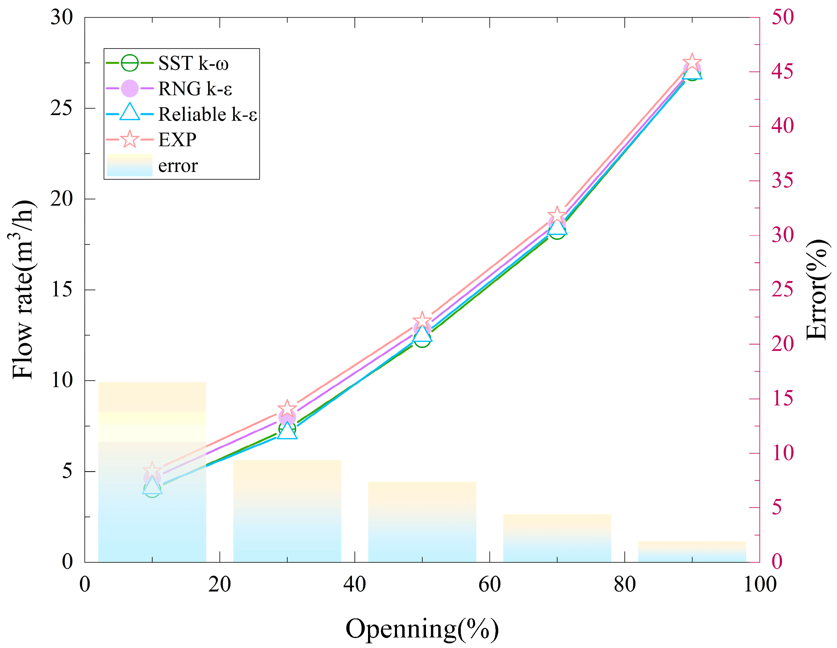
Numerical simulations of the pilot-operated control valve’s flow were conducted using the Realizable k-ε, RNG k-ε, and SST k-ω turbulence models. Comparison with flow test results showed that the RNG k-ε model had the best agreement, with a deviation of less than 10%.

(2)

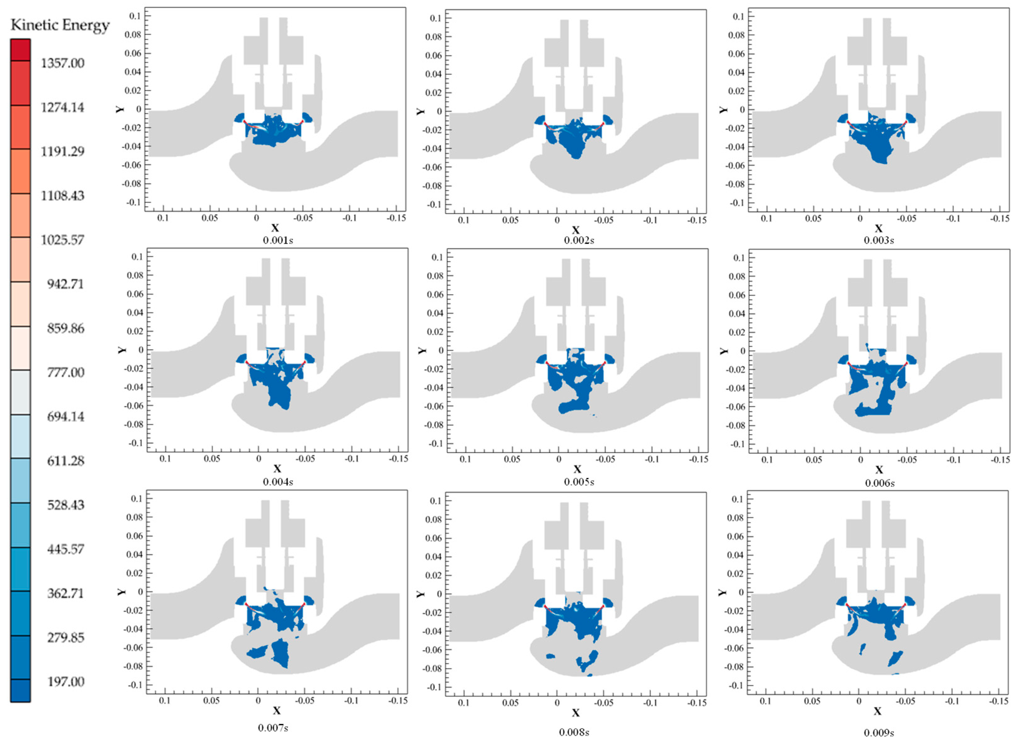
The primary instability factors for the pilot-operated control valve’s core assembly include flow separation, backflow, and vortex formation at the throttling area of the valve core. The peak fluid excitation frequencies experienced by the valve core at typical openings ranged from 100 to 300 Hz, with the fluid excitation force at 70% opening showing a wide frequency band, with harmonic components reaching up to 1000 Hz.

(3)

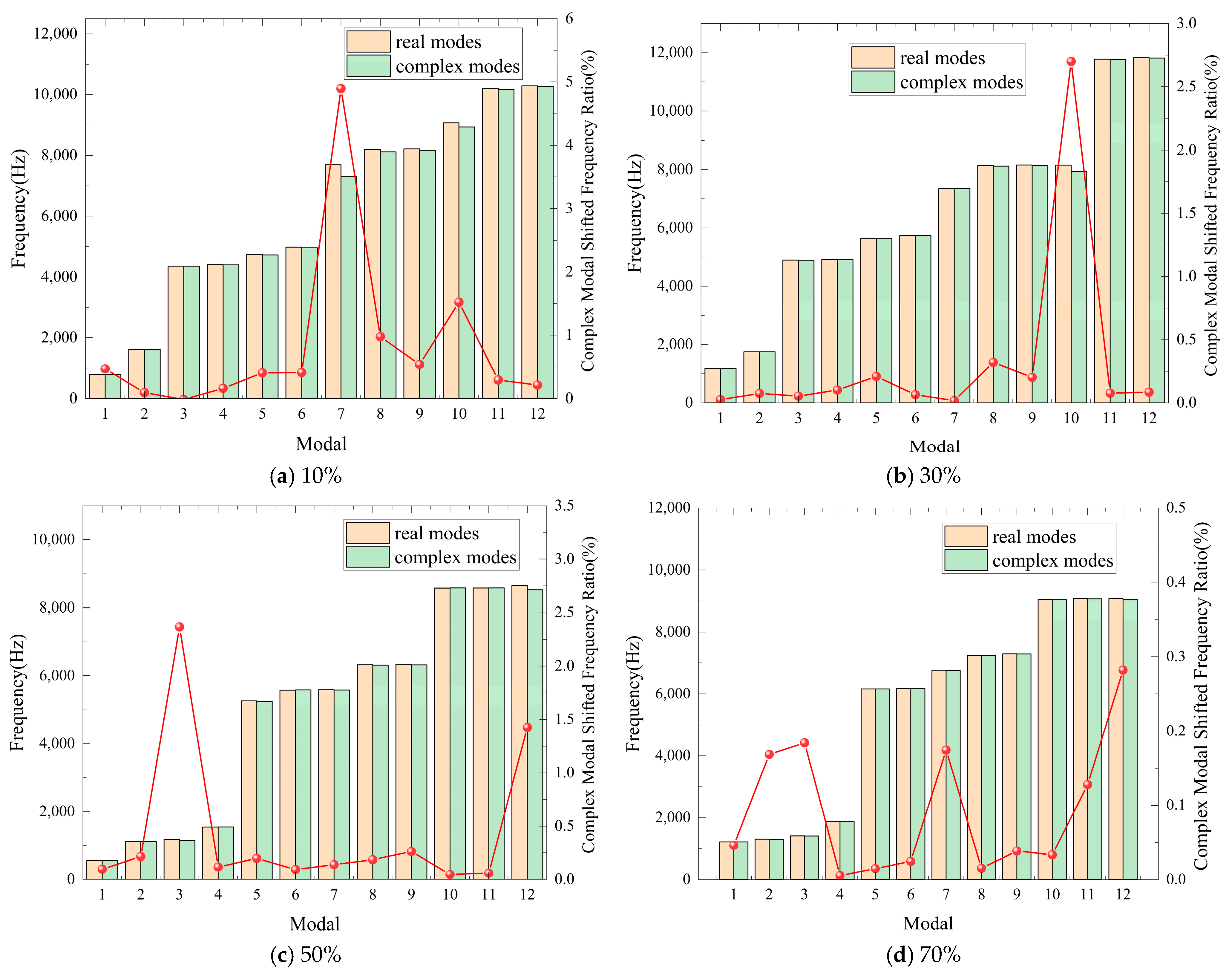
The damping effect caused by the nonlinear relationship in the valve core assembly results in a lower complex modal frequency compared to the real modal frequency. At 10%, 30%, 50%, and 70% openings, the maximum shifts in the complex modal frequency were 4.89%, 2.7%, 1.42%, and 0.46%, respectively. Overall, the complex modal shifts remained small, all under 5%.

(4)

The stability coefficient for the valve core assembly across all modal orders was negative, indicating the relative stability of the valve core system. The stability coefficient of the lower-order modes was near zero, especially for the first-order mode, where critical stability conditions can occur. The stability coefficient showed a negative correlation with the modal order, suggesting that the structure remains relatively stable and safe under high-frequency excitation.

(5)

The modal damping ratios for the valve core assembly’s damping system were greater than 0 but significantly less than 1 across all modal orders, indicating an underdamped state. Under fluid excitation, vibrations gradually decay, and the logarithmic decay rate followed a consistent trend, suggesting the system remains relatively stable. The damping ratio of the first mode was close to 0, and excitation at the first mode frequency could lead to critical stability issues.

(6)

A comparison between the modal frequencies of the valve core assembly and the peak excitation frequencies from the fluid showed that at a 70% opening, the peak excitation frequency reached 959 Hz. At openings of 50% and 70%, the first-order modal frequencies of the valve core assembly were close to the resonance range of the fluid excitation frequency, making resonance likely.

References

1. Jiang, Q.; Li, J.; Wang, P. Study on control characteristics of a nuclear power plant with coupled heat-pipe reactor and sCO2 Brayton cycle. Nucl. Eng. Des. 2025, 432, 113819. [Google Scholar] [CrossRef]
2. Guillen, D.P. Review of passive heat removal strategies for nuclear microreactor systems. Nucl. Technol. 2023, 209, S21–S40. [Google Scholar] [CrossRef]
3. Hajar, I.; Kassim, M.; Minhat, M.S.; Azmi, I.N. Optimal efficiency on nuclear reactor secondary cooling process using machine learning model. Int. J. Electr. Comput. Eng. 2024, 14, 6287–6299. [Google Scholar] [CrossRef]
4. Guo, F.; Lyu, Y.; Duan, Z.; Fan, Z.; Li, W.; Chen, F. Analysis of Regulating Valve Stem Fracture in a Petrochemical Plant. Processes 2023, 11, 1106. [Google Scholar] [CrossRef]
5. Zhou, C.L.; Yan, A.J.; Wei, X.; Fan, Z.D.; Zhu, L. Fracture Failure Analysis of a High-Pressure Bypass Valve Stem. J. Fail. Anal. Prev. 2023, 23, 1038–1045. [Google Scholar] [CrossRef]
6. Jin, H.; Zheng, Z.; Ou, G.; Zhang, L.; Rao, J.; Shu, G.; Wang, C. Failure analysis of a high pressure differential regulating valve in coal liquefaction. Eng. Fail. Anal. 2015, 55, 115–130. [Google Scholar] [CrossRef]
7. Chen, F.-q.; Cai, Q.-r.; Wei, X.-y.; Xu, Q.; Zhu, Z.-j.; Liu, W.-k.; Fan, X.-f. Study on suppression of flow-induced noise in gas turbine fuel control valves. Flow Meas. Instrum. 2025, 104, 102904. [Google Scholar] [CrossRef]
8. Wang, P.; Liu, Y. Unsteady flow behavior of a steam turbine control valve in the choked condition: Field measurement, detached eddy simulation and acoustic modal analysis. Appl. Therm. Eng. 2017, 117, 725–739. [Google Scholar] [CrossRef]
9. Wang, P.; Liu, Y. Influence of a circular strainer on unsteady flow behavior in steam turbine control valves. Appl. Therm. Eng. 2017, 115, 463–476. [Google Scholar] [CrossRef]
10. Wei, A.-b.; Gao, R.; Zhang, W.; Wang, S.-h.; Zhou, R.; Zhang, X.-b. Computational fluid dynamics analysis on flow-induced vibration of a cryogenic poppet valve in consideration of cavitation effect. J. Zhejiang Univ.-Sci. A 2022, 23, 83–100. [Google Scholar] [CrossRef]
11. Zhang, Y.; He, C.; Li, P.; Qiao, H. Numerical and experimental investigation of flow induced vibration of an ejector considering cavitation. J. Appl. Fluid Mech. 2023, 17, 251–260. [Google Scholar]
12. Jin, H.; Xu, H.; Zhang, J.; Wang, C.; Liu, X. Fluid–Structure Coupling Analysis of the Vibration Characteristics of a High-Parameter Spool. Fluids 2025, 10, 105. [Google Scholar] [CrossRef]
13. Duan, Y.; Revell, A.; Sinha, J.; Hahn, W. A computational fluid dynamics (CFD) analysis of fluid excitations on the spindle in a high-pressure valve. Int. J. Press. Vessel. Pip. 2019, 175, 103922. [Google Scholar] [CrossRef]
14. Zeid, A.; Shouman, M. Flow-Induced Vibration on the Control Valve with a Different Concave Plug Shape Using FSI Simulation. Shock Vib. 2019, 2019, 8724089. [Google Scholar] [CrossRef]
15. Zhang, G.; Wang, W.W.; Wu, Z.Y.; Chen, D.S.; Kim, H.D.; Lin, Z. Effect of the opening degree on evolution of cryogenic cavitation through a butterfly valve. Energy 2023, 283, 128543. [Google Scholar] [CrossRef]
16. Yang, H.; Wang, W.; Lu, K.; Chen, Z. Cavitation reduction of a flapper-nozzle pilot valve using continuous microjets. Int. J. Heat Mass Transf. 2019, 133, 1099–1109. [Google Scholar] [CrossRef]
17. Wang, H.; Hu, F.; Kong, X.; Chen, S. Pressure fluctuation of steam on the disc in a triple eccentric butterfly valve. SN Appl. Sci. 2020, 2, 1193. [Google Scholar] [CrossRef]
18. Xu, D.; Ge, C.; Li, Y.; Liu, Y. Evaluation the possibility of vortex-induced resonance for a multistage pressure reducing valve. PLoS ONE 2022, 17, e0266414. [Google Scholar] [CrossRef] [PubMed]
Figure 1. Geometric model of the pilot-operated control valve.
Actuators 14 00372 g001
Figure 2. Structural diagram of the sleeve.
Actuators 14 00372 g002
Figure 3. Flow domain model.
Actuators 14 00372 g003
Figure 4. Inlet pressure monitoring curves of the control valve under five different mesh schemes.
Actuators 14 00372 g004
Figure 5. Computational mesh.
Actuators 14 00372 g005
Figure 6. Experimental testing system 1. Water tank 2 and 6. Butterfly valve 3. Check valve 4. Pump 5. Spherical flexible joint 7, 9, 13, and 18. Electric globe valve 8. Pressure stabilizing tank 10 and 12. Manual globe valve 11. Solenoid valve 14. Tested control valve 15. Back pressure valve 16. Back pressure valve 17. Collection tank 19. Pressure relief valve.
Actuators 14 00372 g006
Figure 7. The experimental testing.
Actuators 14 00372 g007
Figure 8. Comparisons between simulations by different turbulence models and the experimental results of the mass flow rate.
Actuators 14 00372 g008
Figure 9. Distribution of pressure inside the valve.
Actuators 14 00372 g009
Figure 10. Distribution of velocity inside the valve.
Actuators 14 00372 g010
Figure 11. Distribution of turbulent kinetic energy inside the valve.
Actuators 14 00372 g011
Figure 12. Time and frequency domain plots of fluid forces on the valve spool.
Actuators 14 00372 g012
Figure 13. Geometry model and computational mesh.
Actuators 14 00372 g013
Figure 14. Mesh independence verification of modal analysis.
Actuators 14 00372 g014
Figure 15. First 12 mode shapes of the control valve core assembly.
Actuators 14 00372 g015
Figure 16. Comparison of the real and complex modal frequencies at different openings.
Actuators 14 00372 g016
Figure 17. Comparison of stability coefficients at different valve openings.
Actuators 14 00372 g017
Figure 18. Comparison of Damping Ratios at Different Valve Openings.
Actuators 14 00372 g018
Figure 19. Comparison of logarithmic decrement at different valve openings.
Actuators 14 00372 g019
Figure 20. Comparison of modal frequency and fluid forces frequency.
Actuators 14 00372 g020