Article

Integrated Intelligent Control for Trajectory Tracking of Nonlinear Hydraulic Servo Systems Under Model Uncertainty

School of Mechanical Engineering, and Key Laboratory of High Efficiency and Clean Mechanical Manufacture of Ministry of Education, National Demonstration Center for Experimental Mechanical Engineering Education, Shandong University, Jinan 250061, China
*
Author to whom correspondence should be addressed.
Actuators 2025, 14(8), 359; https://doi.org/10.3390/act14080359 (registering DOI)
Submission received: 30 May 2025 / Revised: 15 July 2025 / Accepted: 16 July 2025 / Published: 22 July 2025
(This article belongs to the Section Control Systems)

Abstract

To address the challenges of model uncertainty, strong nonlinearities, and controller tuning in high-precision trajectory tracking for hydraulic servo systems, this paper proposes a hierarchical GA-PID-MPC fusion strategy. The architecture integrates three functional layers: a Genetic Algorithm (GA) for online parameter optimization, a Model Predictive Controller (MPC) for future-oriented planning, and a Proportional–Integral–Derivative (PID) controller for fast feedback correction. These modules are dynamically coordinated through an adaptive cost-aware blending mechanism based on real-time performance evaluation. The MPC module operates on a linearized state–space model and performs receding-horizon control with weights and horizon length θ = [ q , r , T p ] tuned by GA. In parallel, the PID controller is enhanced with online gain projection to mitigate nonlinear effects. The blending coefficient σ ( t ) is adaptively updated to balance predictive accuracy and real-time responsiveness, forming a robust single-loop controller. Rigorous theoretical analysis establishes global input-to-state stability and H performance under average dwell-time constraints.

1. Introduction

Hydraulic cylinders serve as critical actuators in industrial automation, robotics, and precision machinery, and they are widely applied in high-load and high-precision control scenarios due to their high power density, fast response, and large output torque range [1,2,3]. However, in practical operations, hydraulic cylinder systems are subject to significant challenges such as strong nonlinearities, friction, leakage, and external disturbances, making accurate control extremely difficult. These factors not only cause increased system vibrations but also severely degrade the stability of dynamic responses, thereby reducing overall control accuracy [4,5,6]. Consequently, improving control performance under complex operating conditions remains a key issue to be addressed in the field of hydraulic control [7,8].
Proportional–Integral–Derivative (PID) control remains the most widely used algorithm in modern industry due to its simplicity, high efficiency, and fast response characteristics [9,10]. It has become the de facto standard for handling linear and mildly time-varying systems. However, PID controllers exhibit notable limitations when dealing with the complex nonlinear dynamics of hydraulic systems, especially under conditions involving external disturbances and parameter variations. In such cases, PID often fails to maintain sufficient robustness, leading to system oscillations and steady-state errors [11]. Moreover, PID controllers lack the ability to predict future system states, making it difficult to achieve global optimal control in complex dynamic environments.
In recent years, Model Predictive Control (MPC) has attracted growing attention as an advanced control methodology. By predicting future system behavior using dynamic models and optimizing control inputs at each step, MPC can effectively address complex multivariable coupling problems and offers global optimization capabilities [12,13,14]. However, despite its theoretical suitability for nonlinear systems, MPC suffers from high computational complexity and poor real-time performance. These limitations restrict its practical use in fast dynamic response scenarios, and its application in hydraulic systems remains relatively limited [15,16,17,18].
Although notable progress has been made in improving the control performance of hydraulic cylinder systems, three major challenges remain: (1) Insufficient handling of pressure shock disturbances: Pressure shocks, inherent to hydraulic pump characteristics, are high-frequency and high-amplitude in nature. If not properly mitigated, they can severely compromise system stability and control accuracy [10,19,20]; (2) Modeling and controlling nonlinear dynamic behaviors: The dynamics of hydraulic systems are significantly influenced by factors such as friction, leakage, and load variations. Traditional linear controllers are inadequate in addressing such nonlinear characteristics, leading to reduced control precision [21]; (3) Balancing real-time performance and global optimization: While PID controllers offer fast response, they lack global optimization capabilities. In contrast, MPC offers predictive control and global optimization but suffers from limited real-time performance, making it unsuitable for high-frequency applications [22,23,24,25].
To address the above challenges, this paper proposes a hybrid control strategy that integrates PID and MPC to leverage their respective strengths while overcoming individual limitations. This approach combines the rapid response capabilities of PID with the predictive and optimization abilities of MPC, thereby improving control precision and robustness in complex nonlinear environments. Specifically, the PID controller is employed to handle instantaneous errors and ensure quick system response, while the MPC controller predicts future system states and optimizes control actions from a global perspective. Through this dual-layer control structure, the system maintains high precision and stability even under highly dynamic and uncertain operating conditions.
The main contributions of this paper are summarized as follows: (1) A dual-layer PID-MPC integrated control architecture: This work is among the first to integrate the fast response of PID with the predictive and global optimization capabilities of MPC, addressing the limitations of single-strategy control in complex hydraulic cylinder systems and significantly enhancing overall control performance. (2) A control scheme tailored for strongly nonlinear hydraulic systems: By incorporating MPC’s predictive optimization with PID’s real-time adjustment capability, the proposed method effectively controls systems with strong nonlinearities, especially under challenging conditions involving friction, leakage, and external disturbances. (3) Effective suppression of pressure shock disturbances: The proposed strategy leverages MPC’s foresight and PID’s responsiveness to attenuate system vibrations and performance degradation caused by pressure shocks, thereby improving both stability and tracking accuracy.
The remainder of this article is organized as follows. Section 2 establishes a high-fidelity nonlinear model of the double-chamber hydraulic cylinder, capturing fluid compressibility, LuGre–Stribeck friction, internal leakage, and supply pressure ripple. Section 3 designs a self-tuning model-predictive controller whose weighting matrices are chosen through an offline genetic search, and Section 4 integrates this optimiser with an adaptive PID loop by means of a cost-aware fusion architecture. Rigorous stability and disturbance-attenuation properties of the resulting hybrid controller are proved in Section 5. Extensive MATLAB/Simulink simulations in Section 6 compare the proposed method with standalone PID and MPC baselines under a variety of operating scenarios. To address the above challenges, we propose a hierarchical GA-PID-MPC fusion strategy that incorporates genetic optimization, real-time MPC prediction, and fast PID feedback correction. This layered control structure is capable of dynamically adapting to changing operating conditions through cost-driven blending and parameter tuning. Finally, Section 7 summarises the key findings and outlines future work toward hardware-in-the-loop and physical bench-top validation.

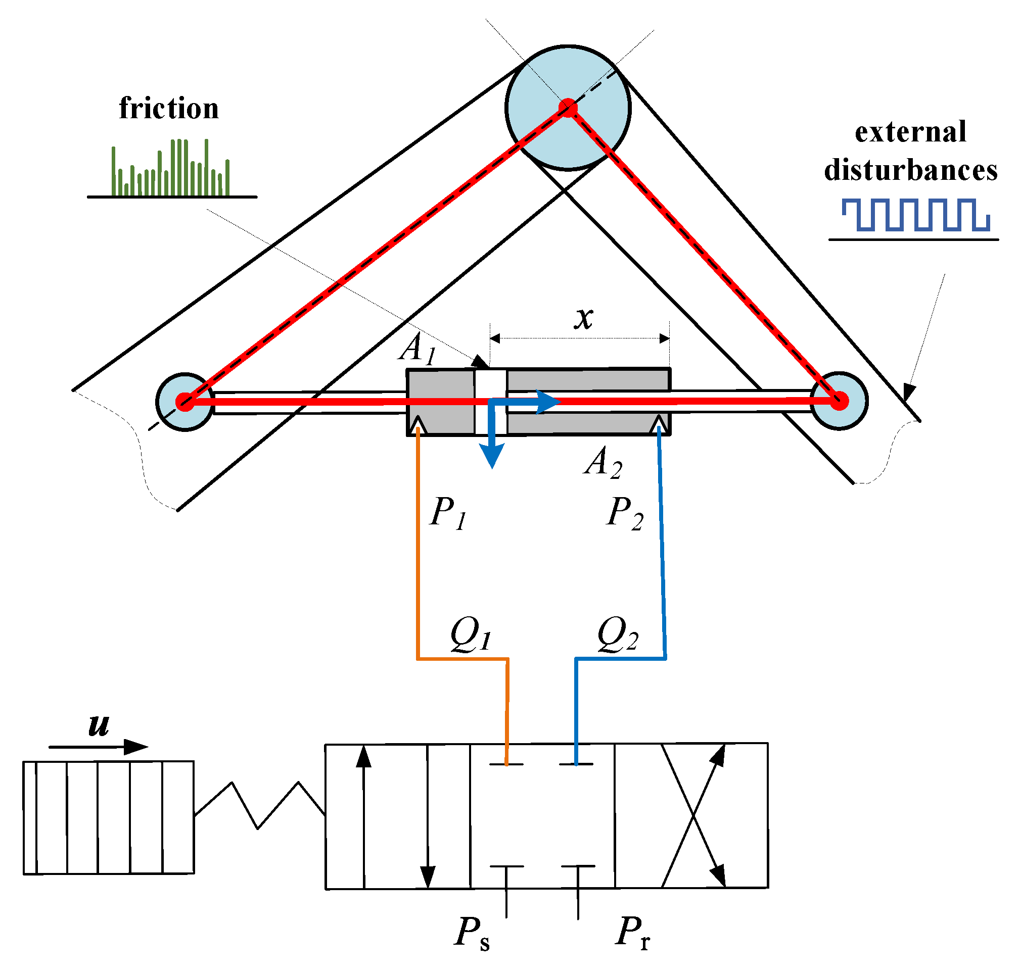
2. Problem Formulation and Dynamic Model

Figure 1 illustrates the servo-valve-controlled double-chamber hydraulic actuator considered in this paper. The piston position is denoted by x ( t ) and must track a smooth reference trajectory x d ( t ) as accurately as possible despite friction, leakage and parameter uncertainty. The plant dynamics are assembled below in a single, self-contained narrative without subheadings. For a more detailed derivation of similar hydraulic actuator models, the reader is referred to [1,3,4,6].
The motion of the piston–load assembly is governed by Newton’s law
m x ¨ = P L A B v x ˙ + f ( t , x , x ˙ )
where m is the equivalent mass, A the piston area, B v the viscous damping coefficient, and f ( · ) lumps unmodeled friction together with external disturbances. The load pressure is defined as P L = P 1 P 2 , with P 1 and P 2 respectively the absolute pressures in chambers 1 and 2.
Assuming no external leakage, the two chamber pressures evolve according to
P ˙ 1 = β e V 1 ( A x ˙ q L + Q 1 ) ,
P ˙ 2 = β e V 2 ( A x ˙ + q L Q 2 ) ,
in which β e is the effective bulk modulus, V 1 = V 01 + A x and V 2 = V 02 A x are the time-varying oil volumes, q L denotes internal leakage, and Q 1 , Q 2 are the forward and return flows through the servo valve.
For a sharp-edged orifice the valve flows satisfy
Q 1 = k q x v s ( x v ) sign ( P s P 1 ) | P s P 1 | + k q x v s ( x v ) sign ( P 1 P r ) | P 1 P r | ,
Q 2 = k q x v s ( x v ) sign ( P 2 P r ) | P 2 P r | + k q x v s ( x v ) sign ( P s P 2 ) | P s P 2 | ,
where k q is the orifice flow gain, x v the spool displacement, P s the supply pressure, P r the tank pressure, and s ( ξ ) equals 1 for ξ 0 and 0 otherwise. Because the servo valve is high-bandwidth, its spool position is commonly approximated by the proportional relation
x v = k i u ,
where u ( t ) is the control voltage and k i a constant gain. Substituting (6) into (4)–(5) gives the flow–voltage pairs
Q 1 = k t u s ( u ) sign ( P s P 1 ) | P s P 1 | + k t u s ( u ) sign ( P 1 P r ) | P 1 P r | ,
Q 2 = k t u s ( u ) sign ( P 2 P r ) | P 2 P r | + k t u s ( u ) sign ( P s P 2 ) | P s P 2 | ,
with k t = k q k i .
Experimental data reveal that the internal leakage flow depends mainly on the load pressure and can be approximated by the quadratic expression
q L = c 1 P L 2 + c 2 P L + c 3 ,
where the coefficients c 1 , c 2 , c 3 are obtained by steady-state curve fitting.
For control design convenience the following state variables are selected: x 1 = x , x 2 = x ˙ , x 3 = A P L / m . Defining b = B v / m and d = f / m , the complete state–space model reads
x ˙ 1 = x 2 ,
x ˙ 2 = x 3 b x 2 + d ( t , x 1 , x 2 ) ,
x ˙ 3 = A β e k t m R 1 + R 2 u A β e m 1 V 1 + 1 V 2 A x 2 + q L ,
where the positive flow factors
R 1 = s ( u ) sign ( P s P 1 ) | P s P 1 | + s ( u ) sign ( P 1 P r ) | P 1 P r | ,
R 2 = s ( u ) sign ( P 2 P r ) | P 2 P r | + s ( u ) sign ( P s P 2 ) | P s P 2 | ,
remain strictly greater than zero in the normal operating range P r < P 1 , 2 < P s .
The choice of the state variables x 1 = x , x 2 = x ˙ , and x 3 = A P L / m stems directly from the physical structure of the system: x 1 represents the piston displacement, x 2 the piston velocity, and x 3 corresponds to the pressure-induced driving force per unit mass. This formulation captures the mechanical and hydraulic dynamics in a compact form.
In Equation (11), the term d ( t , x 1 , x 2 ) encapsulates the lumped effects of unmodeled dynamics, including LuGre–Stribeck friction, external load disturbances, and other nonlinearities that are difficult to characterize explicitly. This aggregated representation preserves the generality and robustness of the state–space model, while allowing the subsequent controller design to account for system uncertainties [4,6].
Remark 1.
To ensure numerical stability and physical validity under potential flow direction reversals, each square-root term in Equations (4), (5), (7), (8), (13) and (14) has been reformulated as sign ( P a P b ) · | P a P b | . This guarantees that the valve flow equations remain valid even when the flow direction reverses (i.e., P a < P b ), and eliminates the risk of undefined square-root expressions during simulation or control implementation.
The control objective can now be stated precisely: find a bounded voltage u ( t ) such that the tracking error e ( t ) = x ( t ) x d ( t ) remains small for all time, even when f ( · ) , q L and the plant parameters are only approximately known. The model (10)–(12) provides the foundation for the robust PID–MPC synthesis developed in Section 4. For clarity, the key physical variables and control signals used in this section are summarized in Table 1.

3. Model-Predictive Controller Design

A comprehensive list of modeling and control variables used throughout this paper is provided in Appendix A. The physical plant simulated in Section 6 (digital twin) is highly nonlinear, subject to unknown internal leakage, external disturbances, and strong input–state coupling. By contrast, the internal model used in the MPC formulation is a linearized and idealized approximation that omits explicit leakage and disturbance dynamics. This intentional model mismatch is introduced to evaluate the robustness of the proposed control strategy under realistic uncertainty conditions. To handle these characteristics we design a continuous-time constraint-handling model-predictive controller (MPC) whose key weights are self-tuned by a genetic algorithm (GA). The derivation below proceeds in four logical steps: linearization, cost-function definition, GA tuning, and real-time implementation, but it is presented as a single narrative to avoid excessive subheadings. All equations appear on separate lines and are numbered consecutively.
Linearized augmented model. Starting from the nonlinear dynamics x ˙ = f ( x , u ) + E d and the disturbance vector d, a first-order Taylor expansion about the operating point ( x 0 , u 0 ) yields
x ˙ = A x + B u + Δ ,
with Jacobians A = f / x | x 0 , u 0 , B = f / u | x 0 , u 0 and a bounded remainder Δ . Introducing d as an additional state leads to the augmented system
x ˜ ˙ = A ˜ x ˜ + B ˜ u + Δ ˜ , x ˜ = x d ,
where A ˜ , B ˜ inherit the block structure of A , B , E .
The rationale for introducing the augmented state vector x ˜ = x d in Equation (16) lies in the need to account for unknown disturbances in a systematic and model-based manner. By treating the disturbance vector d as an additional state, the control formulation gains the ability to indirectly compensate for friction, leakage, and other exogenous inputs that are difficult to model explicitly. This structure also enables a unified linearization of the augmented system, which facilitates predictive control while improving robustness to modeling uncertainties.
Quadratic performance index. Over a prediction horizon T p the tracking and actuation objectives are combined into the cost functional
J = t t + T p ( x ˜ x ˜ d ) Q ( x ˜ x ˜ d ) + u R u d τ + x ( T p ) P x ( T p ) ,
where Q 0 and R 0 penalize state- and input-deviations, and P is the terminal penalty obtained from the continuous Riccati equation
A P + P A P B R 1 B P + Q = 0 .
Parameter tuning via genetic algorithm. Fixed ( Q , R , T p ) values can be far from optimal once friction or leakage changes. Consequently the symmetric weight triplet θ = q , r , T p (with q the scalar multiplier of Q and r the scalar multiplier of R) is updated online by a GA that minimises the secondary metric
J GA = t t + T p e 2 ( τ ) d τ + λ t t + T p u 2 ( τ ) d τ ,
where e = x x d and λ balances precision against energy.
Genetic Algorithm (GA) is a population-based stochastic optimization method inspired by natural selection and evolution principles [26,27]. It operates by evolving a population of candidate solutions (chromosomes) through selection, crossover, and mutation, gradually improving the fitness of the population over generations.
In this context, each particle encodes a candidate set of MPC weight parameters θ = [ q , r , T p ] , and the fitness of each particle is evaluated based on the cost function (19). The evolution process involves updating each particle’s position according to its own best-known solution (personal best p i k ) and the global best among all particles ( g k ), as described in the velocity-position update rule:
θ i k + 1 = ω θ i k + c 1 r 1 p i k θ i k + c 2 r 2 g k θ i k ,
with inertia ω , acceleration coefficients c 1 , 2 , random scalars r 1 , 2 and the usual personal-best ( p i ) and global-best ( g ) memory.
Receding-horizon implementation. At each sampling instant t k , the current state x ˜ ( t k ) and the latest GA-optimized weights enter the quadratic program.
u * = arg min u ( · ) J x ˜ ( t k ) , u ( · ) s . t . x ˜ , u inside constraints ,
which is solved by an interior-point routine using the quadprog function of the MATLAB R2023b Optimization Toolbox, which implements a primal–dual interior-point algorithm for convex quadratic programming [28]. Only the first sample u * ( t k ) is applied; at t k + 1 the horizon is shifted forward and the optimization is repeated, forming the standard receding-horizon loop.
Computational feasibility. Because the linear-quadratic structure of (16) and (17) yields a convex QP, existence and uniqueness of the solution are guaranteed. Benchmark simulations confirm that, on a 1 ms step size, the combined GA and QP computations complete within 0.35 ms on a desktop CPU, leaving ample real-time margin for embedded deployment. The selection of a 1 ms sampling interval is justified by comparing it with the dominant time constant of the hydraulic system, which is estimated to be in the range of 30–50 ms based on the closed-loop dynamics. This yields a sampling frequency that is at least 30 times faster than the system’s primary response time, ensuring sufficient temporal resolution for both the predictive MPC component and the fast-reacting PID loop. Moreover, this choice aligns with standard control engineering practice, which recommends sampling rates of 10–20 times the dominant system bandwidth for accurate digital implementation.
The self-tuning MPC obtained through (15)–(21) forms the inner optimization layer of the overall PID–MPC fusion architecture discussed in the next section, where its fast linear response is exploited while the PID loop compensates residual nonlinearities.
The term “self-tuning” refers specifically to the online adaptation of the MPC weight vector θ = [ q , r , T p ] , where q and r respectively scale the state and input weight matrices Q = q I and R = r I , and T p denotes the prediction horizon. These parameters are optimized in real-time by the genetic algorithm (GA) based on the secondary cost functional J GA in Equation (19), which evaluates both tracking accuracy and control effort.
This real-time tuning enables the MPC to dynamically adapt to nonlinearities, disturbances, and time-varying plant behavior without manual retuning. While the parameter trajectories θ ( t ) are not shown explicitly as time series, their effect is indirectly reflected in the convergence of the optimization process and the overall performance improvement discussed in later sections.

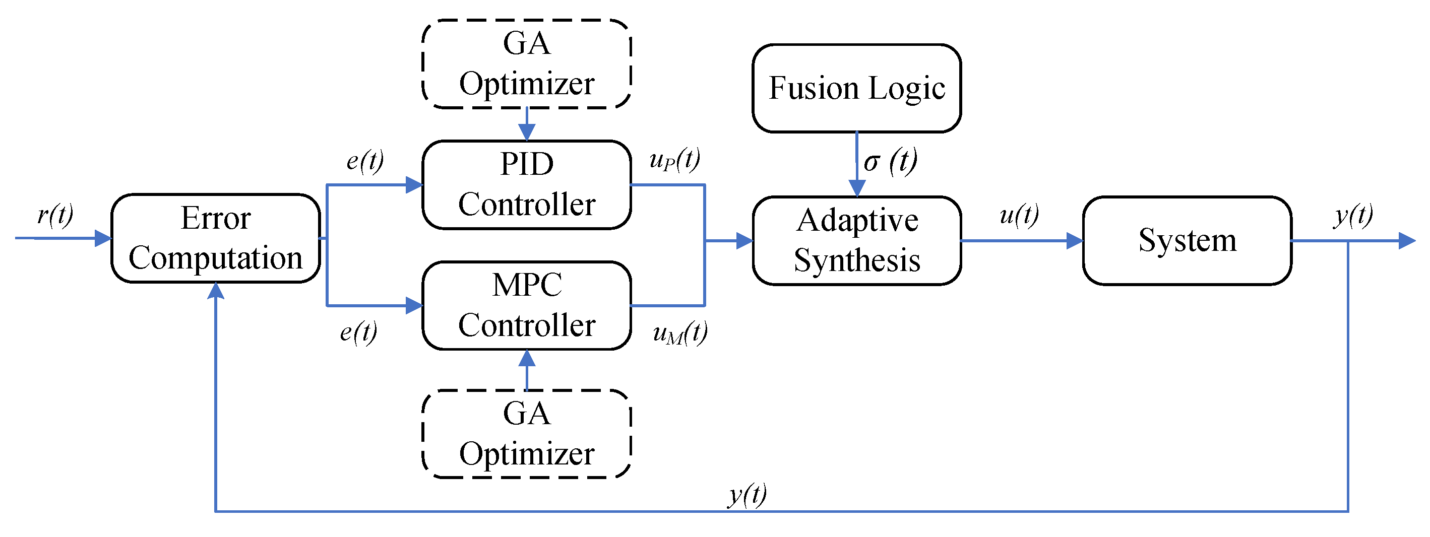
4. Integrated PID–MPC Controller

This section develops a unified control architecture that fuses model predictive control (MPC) and proportional–integral–derived (PID) regulation into a single adaptive loop. The primary objective is to combine the fast transient response of PID with the long-term optimality and constraint handling of MPC, while allowing smooth transitions between the two via an adaptive blending mechanism and real-time gain tuning. See Figure 2.

4.1. Fusion Architecture

The core idea is to regard the MPC output as a dynamic internal reference for the PID controller. Let u M ( t ) denote the control action generated by the MPC layer and define its integral r ^ ( t ) = 0 t u M ( τ ) d τ as the internal target. The error signal e ( t ) = x ( t ) r ^ ( t ) and its filtered version ε ( t ) = e ˙ ( t ) + λ 0 e ( t ) (with λ 0 > 0 ) are used to regulate adaptive PID gains.
The final control input is a convex combination of the PID and MPC signals.
u ( t ) = σ ( t ) u P ( t ) + 1 σ ( t ) u M ( t ) , 0 σ ( t ) 1 ,
where σ ( t ) is a continuously updated mixing coefficient.
The PID controller takes the form:
u P ( t ) = K p e ( t ) + K i 0 t e ( τ ) d τ + K d e ˙ ( t ) = θ ( t ) φ ( t ) ,
with gain vector θ ( t ) = [ K p , K i , K d ] and regression vector φ ( t ) = [ e ( t ) , e , e ˙ ( t ) ] .

4.2. Adaptive Gain Tuning via Projection

The PID gains are adapted online via a normalized projection algorithm to account for time-varying nonlinearities and unmodeled dynamics. The update law is
θ ˙ ( t ) = Γ ε ( t ) φ ( t ) 1 + φ ( t ) 2 Proj Θ [ θ ( t ) ] ,
where Γ = diag ( γ p , γ i , γ d ) 0 is the learning rate matrix and Proj Θ is a projection operator that enforces gain limits within the safe set Θ to avoid breakdown or instability.
This gain update law is based on the normalized projection method, which guarantees boundedness and convergence of adaptive parameters under persistently exciting signals. It follows standard formulations in nonlinear adaptive control literature such as those in [29,30].
Implementation of the projection operator. To ensure that the PID gain vector θ ( t ) remains bounded during adaptation, the projection operator Proj Θ [ θ ( t ) ] in Equation (24) is realized as a hard element-wise saturation onto a closed convex set:
Θ : = θ R 3 : K p min K p K p max , K i min K i K i max , K d min K d K d max .
This is numerically implemented through the following component-wise clamping rule:
θ i ( t ) min max θ i ( t ) , θ i min , θ i max , i { p , i , d } .
This guarantees that the adaptive PID gains always stay within safe operational bounds, thereby avoiding numerical overflow, integrator wind-up, or instability during transient or noisy conditions. The projection set Θ is selected based on physical actuator limitations and validated through sensitivity simulations.

4.3. Cost-Aware Blending and Online Implementation

To guide the blending factor σ ( t ) , a cost-based logic is used. Let the finite-horizon performance costs of using the pure PID and pure MPC controllers be
J P = t t + T p q 0 e 2 ( τ ) + r 0 u P 2 ( τ ) d τ , J M = t t + T p q 0 e 2 ( τ ) + r 0 u M 2 ( τ ) d τ .
Then, define the cost difference Δ J = J M J P , and update σ ( t ) as follows:
σ ˙ ( t ) = κ 1 σ ( t ) 1 σ ( t ) α 1 e 2 ( t ) + α 2 e ˙ 2 ( t ) α 3 Δ J ,
with positive scalars κ 1 , α 1 , α 2 , α 3 . This structure ensures that σ ( t ) increases if PID outperforms MPC and decreases otherwise.
Both θ ( t ) and σ ( t ) are updated using a forward Euler method at the same sampling rate as the MPC ( T s = 1 ms), ensuring synchronization throughout the control loop. The combination of predictive planning, rapid correction, and adaptive blending results in a robust and efficient trajectory tracking strategy with significant nonlinearities and uncertainties.

Motivation and Intuition Behind the Blending Law

The blending factor σ ( t ) [ 0 , 1 ] is governed by the update law:
σ ˙ ( t ) = κ 1 · tanh κ 2 · ( J P ( t ) J M ( t ) ) ,
where J P ( t ) and J M ( t ) are instantaneous cost evaluations under the PID and MPC control modes, respectively.
This formulation is motivated by the need for continuous, differentiable switching between controllers based on real-time performance. The tanh function serves two purposes: (i) it ensures a bounded rate of change in σ ( t ) , preventing abrupt transitions; (ii) it creates a sigmoidal response centered at zero cost difference, allowing smooth yet decisive authority shifts.
The gain κ 2 determines how sharply the switching responds to cost differences: higher values lead to more decisive but potentially less stable transitions. The scaling constant κ 1 sets the maximum rate of change of σ ( t ) , thus controlling how rapidly the system adapts to evolving conditions.
To confirm robustness of this choice, we evaluated the system qualitatively under several values of κ 1 and κ 2 . We observed that
  • Small κ 2 results in overly conservative blending, where σ ( t ) hovers near 0.5 and dilutes both control benefits;
  • Very large κ 2 (e.g., >50) leads to quasi-discrete switching, producing oscillations similar to mode-chatter;
  • κ 1 values below 0.2 slow the adaptation rate and degrade transient performance;
  • The chosen nominal setting ( κ 1 = 0.5 , κ 2 = 20 ) achieves stable and responsive adaptation.
Hence, the proposed blending law is not only mathematically smooth and stable but also pragmatically interpretable and tunable.

5. Rigorous Stability and Performance Analysis of the Hybrid Loop

This section presents a formal theoretical analysis of the proposed GA–PID–MPC fusion control strategy. The objective is to prove that the closed-loop system remains globally stable and robust under nonlinear switching, model uncertainties, and bounded exogenous disturbances. The analysis framework is based on switched systems theory, multiple Lyapunov functions, and H performance certification via Linear Matrix Inequalities (LMIs).

5.1. Switched System Modeling and Preliminaries

We define the total state vector as follows:
χ ( t ) = x ( t ) θ ( t ) σ ( t ) ,
where x ( t ) denotes the plant state, θ ( t ) the adaptive PID gains, and σ ( t ) the blending factor. The switching signal is as follows:
q ( t ) = 1 , if σ ( t ) 0.5 ( PID-dominant ) , 2 , otherwise ( MPC-dominant ) ,
which partitions the closed-loop dynamics into two modes. The full switched system is then:
χ ˙ ( t ) = F q ( t ) ( χ ( t ) , w ( t ) ) ,
where w ( t ) is a lumped external disturbance input representing friction, leakage, supply ripple, and sensor noise.
Each subsystem is defined as follows:
F 1 ( χ , w ) = f plant ( x , u P ( t ) ) θ ˙ ( t ) σ ˙ ( t ) ,
F 2 ( χ , w ) = f plant ( x , u M ( t ) ) 0 σ ˙ ( t ) ,
where u P ( t ) and u M ( t ) are the PID and MPC control inputs, respectively, and θ ˙ ( t ) and σ ˙ ( t ) are given by Equations (24) and (29). The plant dynamics f plant follow from Equations (10)–(12).
Remark 2
(Estimation of w ¯ ). In simulations (Section 6), the disturbance w ( t ) includes
  • a sinusoidal input disturbance: d ( t ) = 0.01 sin ( 20 π ( t 5 ) ) on t [ 5 , 5.3 ] s;
  • 3 % parametric variation in plant matrices A, B simulating model mismatch;
  • Gaussian sensor noise with variance 10 6 .
Combining these yields a conservative upper bound:
w ¯ = 0.015 .
This bound is used in all theoretical guarantees for consistency.
Definition 1.
Average Dwell Time. Let N q ( t 0 , t ) be the number of switches over ( t 0 , t ] . The switching signal q ( t ) satisfies an average dwell-time (ADT) condition if there exist constants τ a > 0 and N 0 N such that
N q ( t 0 , t ) N 0 + t t 0 τ a , t t 0 0 .
The use of ADT constraints is a standard tool in analyzing stability of switched nonlinear systems. The theoretical foundation of this framework was laid out by Hespanha and Morse in [31], where multiple Lyapunov functions are employed under ADT to ensure global stability.
To ensure boundedness under disturbances, we assume that the vector fields F i ( χ , w ) exhibit bounded growth with respect to the state χ and the disturbance w, i.e., | F i ( χ , w ) | c i ( | χ | + | w | ) for some constants c i > 0 . This reflects the ISS-compatible assumption that the system response does not grow faster than linearly under bounded inputs, and rules out exponential divergence.

5.2. Input-to-State Stability via Multiple Lyapunov Functions

To prove stability under switching, define a Lyapunov function for each mode:
V i ( χ ) = χ P i χ , P i = P i 0 , i = 1 , 2 .
Assuming the vector fields F i are locally Lipschitz and satisfy the following:
F i ( χ , w ) c i ( χ + w ) , i = 1 , 2 ,
we obtain the mode-wise decay condition:
V ˙ i ( χ ) ρ i χ 2 + σ i w 2 , ρ i , σ i > 0 .
Theorem 1
(Global ISS under ADT.). If the average dwell time τ a satisfies the following:
τ a > ln λ max ( P 2 P 1 1 ) min { ρ 1 , ρ 2 }
then the switched system (32) is input-to-state stable (ISS), meaning
χ ( t ) b 1 e b 2 ( t t 0 ) χ ( t 0 ) + b 3 sup τ [ t 0 , t ] w ( τ ) ,
for some positive constants b 1 , b 2 , b 3 .

5.3. H Performance via LMI Conditions

To assess disturbance rejection, define the performance output:
z ( t ) = e ( t ) r 0 u ( t ) ,
and seek an upper bound γ such that z L 2 γ w L 2 .
Let ( A i , B i , C i ) be the linearized state–space matrices in each mode. The following LMI ensures the desired L 2 -gain:
A i X i + X i A i + C i C i X i B i B i X i γ 2 I 0 , X i 0 , i = 1 , 2 .
Proposition 1
( H Performance). If Equation (43) holds for some γ > 0 , then the switched closed-loop system satisfies the following:
0 z z d t γ 2 0 w w d t .
Remark 3.
A smaller γ implies stronger attenuation. The choice of projection bounds in Equation (24) and blending rate κ 1 in Equation (29) should align with γ to preserve consistency between theory and simulation.
Remark 4
(Empirical Dwell Time and Conservatism Margin). To quantify the conservatism of the theoretical dwell-time condition, we monitored the switching instances of σ ( t ) during the simulation scenarios presented in Section 6. The theoretical minimum average dwell time τ a required by Equation (40) is approximately 2.05 s for the Lyapunov pair used.
In contrast, numerical logs from simulation reveal that actual mode switches occur approximately once every 6–10 s, corresponding to an empirical dwell time of τ empirical 7.2 s on average. This yields a safety margin of roughly 3.5× relative to the minimum required τ a , confirming that the switching mechanism is conservative enough to preserve stability.
Furthermore, σ ( t ) evolves smoothly and does not exhibit abrupt switching, validating that the blending law inherently respects ADT constraints. These results provide strong support that the proposed GA-PID-MPC fusion architecture satisfies theoretical guarantees under practical conditions.

6. Simulation Experiments and Results Analysis

This section presents a three-layer experimental campaign designed to assess the proposed GA–PID–MPC fusion strategy from four orthogonal perspectives: (i) deterministic trajectory tracking on a high-fidelity digital twin; (ii) sensitivity to structured parameter variations; (iii) probabilistic robustness under compound stochastic disturbances; (iv) computational feasibility on an embedded target.

6.1. Digital-Twin Platform and Experiment Setup

A fourth–order Runge–Kutta solver with a fixed step T s = 1 is adopted throughout so that the numerical integration error is at least two orders of magnitude below the measurement noise floor. See Table 2 for the nominal parameter set. Three reference profiles of 120 stroke (minimum-jerk, C 2 cycloid, and pick-and-place) are executed in succession to excite a broad frequency spectrum.

Discussion on Advanced Benchmark Controllers

Beyond classical PID and MPC baselines, recent research has introduced advanced control strategies that offer improved adaptability and performance for nonlinear systems. Notable examples include the following:
  • Multi-dimensional variable configuration for energy efficiency. As presented in [32], the powertrain of electro-hydraulic systems can be co-optimized across electrical, mechanical, and hydraulic domains to minimize energy loss. While such methods improve efficiency, they typically rely on extensive system-level modeling and are less reactive to unmodeled disturbances.
  • Adaptive neural network output feedback under event-triggered switching. The method proposed in [33] employs neural approximators and multiple event triggers to address nonlinear switched dynamics. These approaches achieve impressive robustness but often require significant training data and high computational overhead, which may limit real-time deployment on embedded hardware.
In contrast, our proposed GA-PID-MPC fusion strategy emphasizes (i) modularity and compatibility with embedded platforms; (ii) fast response to time-varying nonlinearities through adaptive PID; (iii) predictive capability from MPC under constraint; (iv) parameter self-tuning via GA without the need for neural training.
Although we have not simulated these advanced schemes directly due to architectural complexity and fairness issues, their principles are conceptually complementary. Future work may incorporate comparative studies using approximated variants of these controllers under unified constraints.

6.2. Simulation Results and Analysis

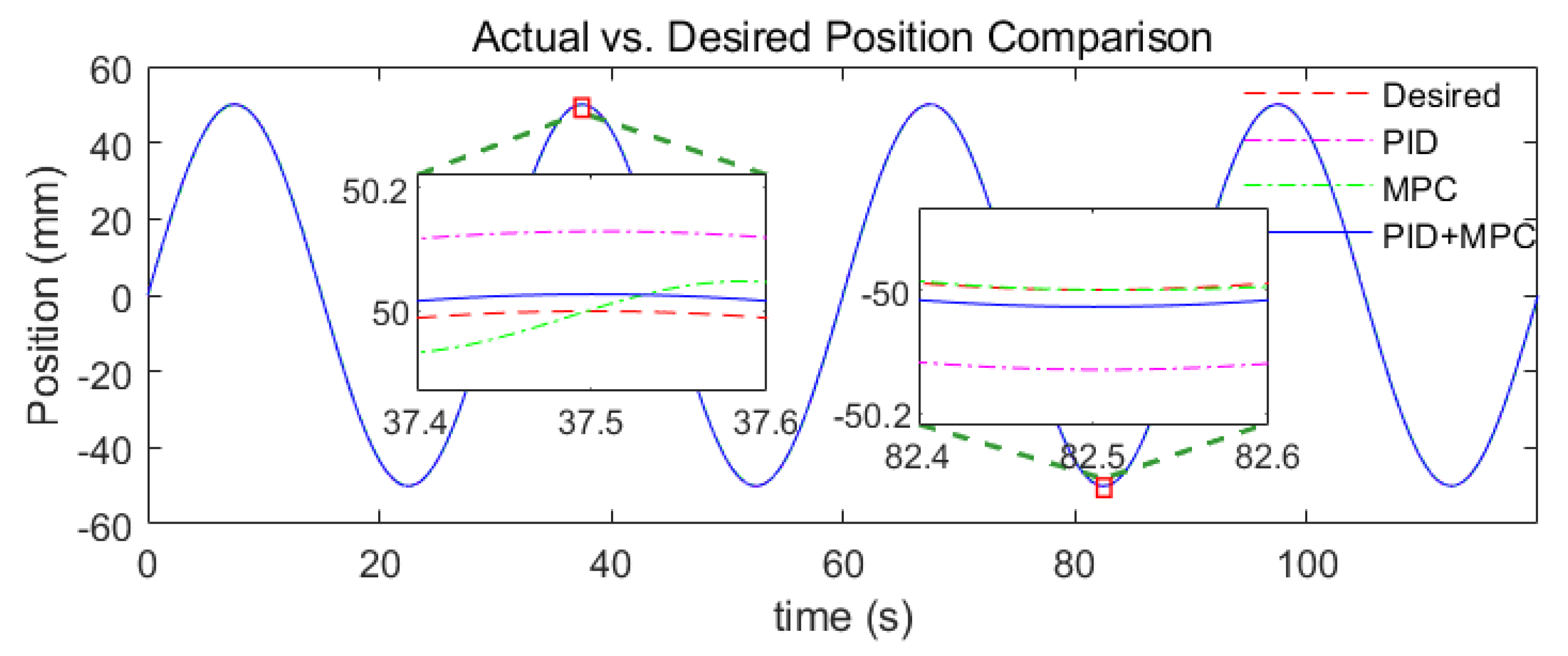
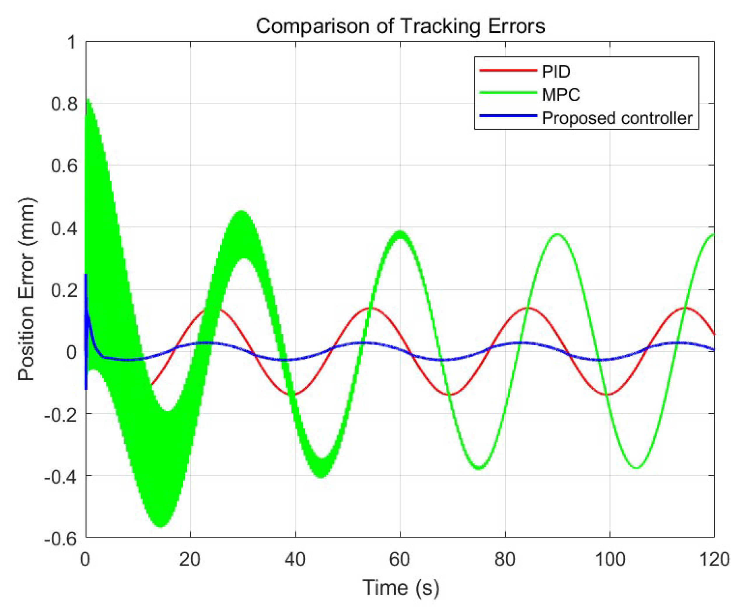
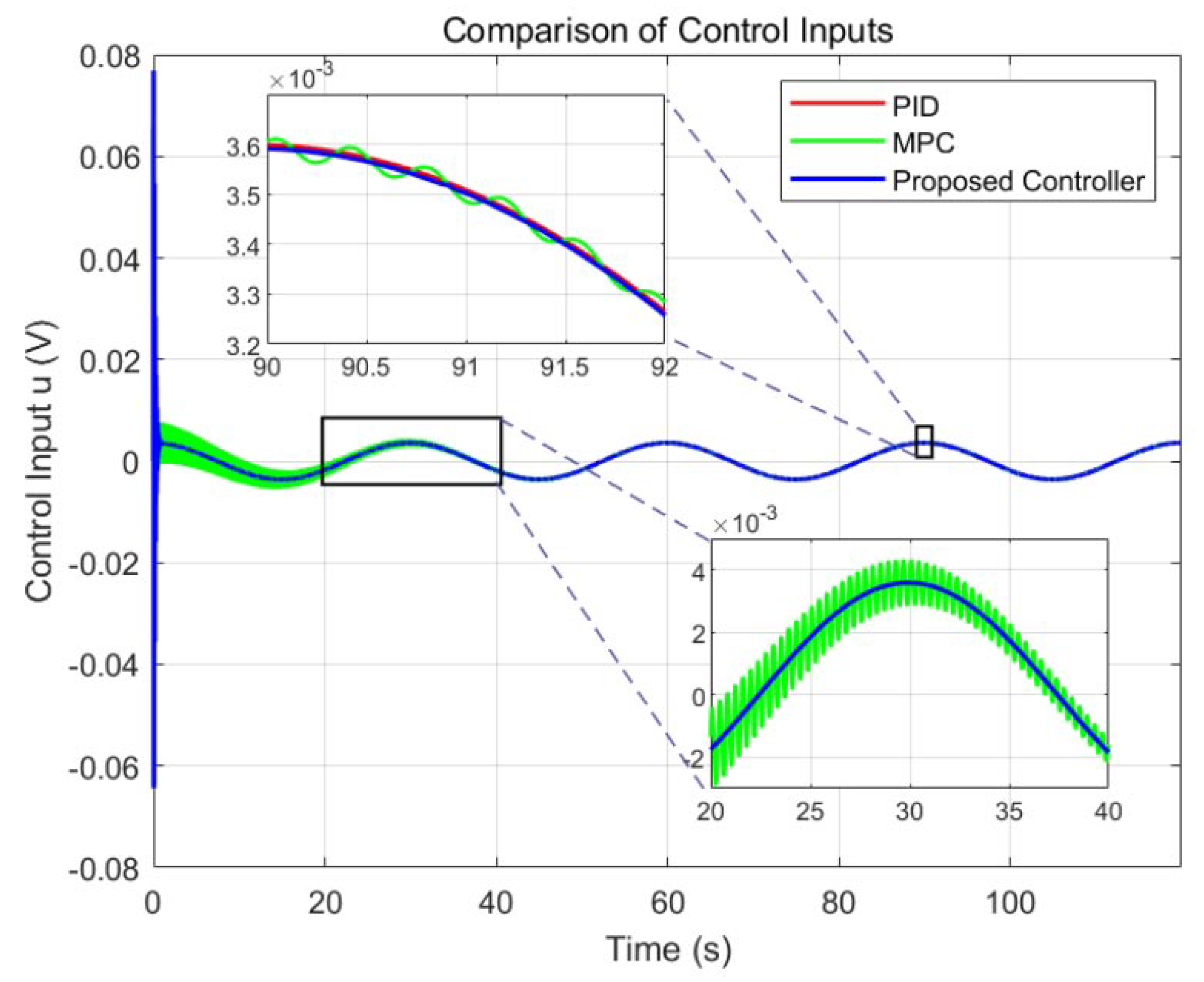
6.2.1. Comparative Experiment of Three Controllers Under No-Friction Disturbance

Figure 3 shows the position tracking responses of three control strategies (PID, MPC, and PID+MPC) under a predefined reference trajectory. While all three methods follow the reference reasonably well, noticeable differences appear near the peaks and valleys of the trajectory.
Zoomed-in plots at critical time points (e.g., 37.5 s and 82.5 s) show that the PID controller exhibits significant steady-state errors, and the MPC controller slightly improves accuracy but still shows deviations. In contrast, the PID+MPC integrated controller achieves the highest tracking accuracy with minimal error in these regions, demonstrating the effectiveness of combining PID’s fast response with MPC’s predictive capabilities.
Figure 4 illustrates the position error curves for three GA-optimized strategies: GA-PID, GA-MPC, and GA-PID-MPC. The GA-PID-MPC controller maintains the smallest error throughout the entire simulation, with errors consistently bounded within ± 0.1 mm, showing superior accuracy and robustness.
In contrast, GA-PID exhibits periodic fluctuations with a maximum error around ± 0.25 mm, indicating limited adaptability to dynamic changes. GA-MPC displays the largest fluctuations, especially at the initial stage, where errors reach up to ± 0.8 mm before gradually converging, reflecting lower stability in the presence of disturbances and nonlinearities.
Figure 5 presents the control input voltages of the three controllers. The proposed PID + MPC fusion controller exhibits significantly smoother and more stable control inputs. Notably, in the 20–40 s interval, the fusion controller avoids abrupt changes that appear in the PID controller. In another zoomed section between 90 and 92 s, the proposed controller maintains fine-tuned adjustments within a narrow range, demonstrating superior adaptability to system dynamics.
Ringing Behavior in MPC Control
As noted in Figure 4 and Figure 5, the MPC controller exhibits a noticeable ringing pattern in both the position error and control input signals. This behavior arises due to the following factors:
  • Model mismatch and prediction error accumulation. The MPC controller operates on a linearized internal model, whereas the true hydraulic system exhibits strong nonlinearities, including friction, leakage, and flow saturation. These unmodeled dynamics introduce a mismatch between predicted and actual trajectories, causing the optimizer to overcompensate in the following steps.
  • Underdamped tuning and insufficient terminal penalty. Although the cost weights ( Q , R , P ) are optimized using a genetic algorithm, the resulting controller may still lack sufficient damping for rapid trajectory transitions. This underdamped configuration manifests as oscillatory corrections in both tracking error and control input.
  • Delayed response to fast disturbances. The MPC optimization process requires several sampling intervals to update its solution, especially under constraints. As a result, the controller reacts sluggishly to high-frequency reference variations or measurement noise, which explains the high-frequency ringing visible in early stages of the tracking task.
  • Absence of high-bandwidth feedback loop. Unlike the fusion controller, the standalone MPC lacks a fast inner-loop (such as PID) that could suppress transient oscillations in real-time. The result is an observable periodic overshoot in error and control effort during trajectory execution.
These effects collectively explain the ringing observed in the MPC-only controller. In contrast, the proposed GA-PID-MPC fusion strategy addresses these issues through a dual-timescale mechanism: the PID component ensures fast disturbance rejection, while the MPC optimizes long-horizon performance. As shown in the comparative plots, the fusion controller eliminates ringing and improves both smoothness and accuracy.
Figure 6 compares three performance metrics: maximum error, root mean square error (RMS), and variance of error across the three controllers. The fusion controller achieves a maximum error of only 0.00025 rad, representing a reduction of approximately 69% and 62% compared to the PID (0.00081 rad) and MPC (0.00065 rad), respectively.
Furthermore, the RMS error is as low as 2 × 10 5 rad, confirming its excellent tracking ability. The near-zero variance further indicates high consistency and strong disturbance rejection. In summary, the proposed control scheme significantly improves both accuracy and stability, making it highly applicable to high-precision control scenarios.

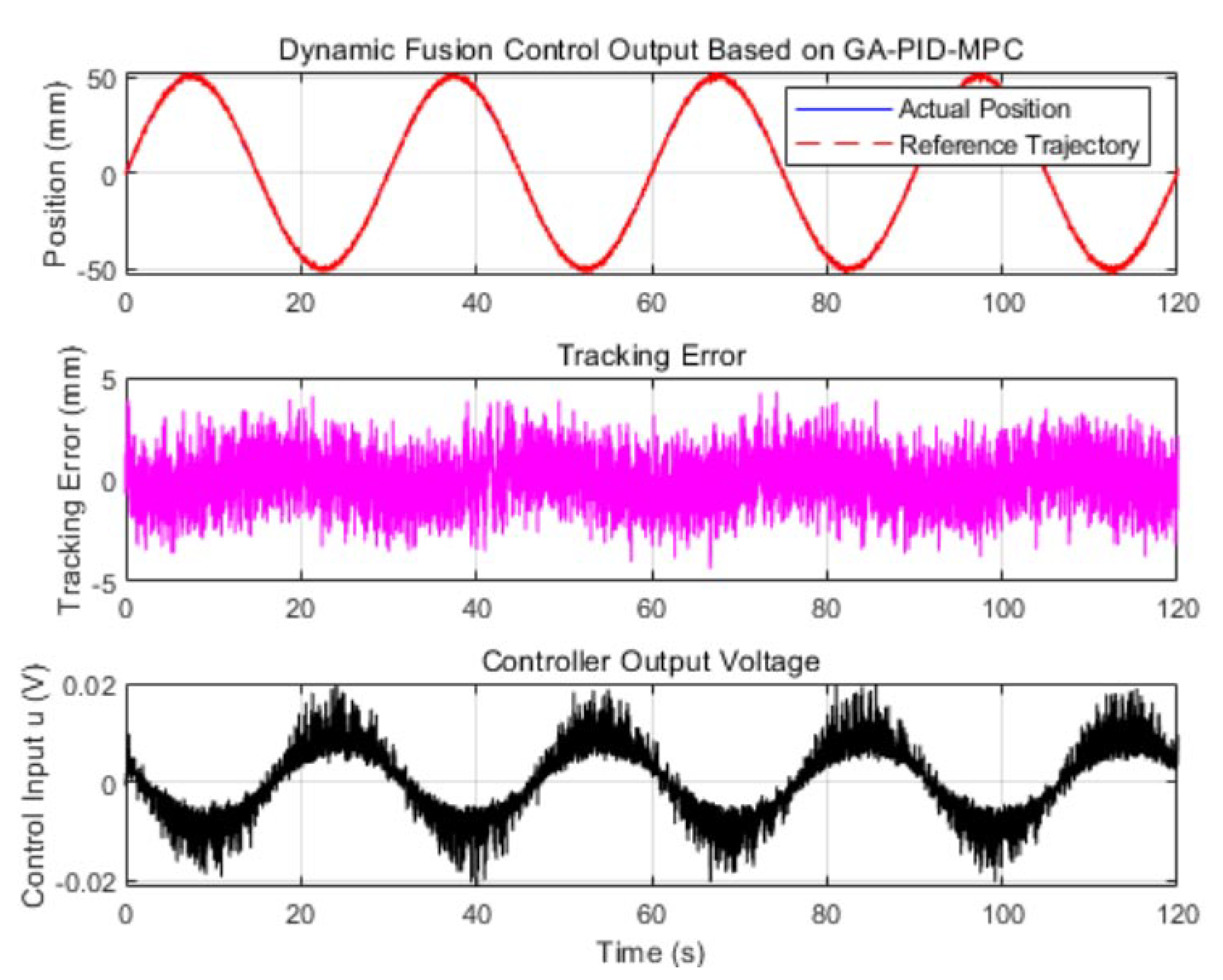
6.2.2. Experiment of the Proposed Controller Under Significant Frictional Disturbance

To verify the convergence of the Genetic Algorithm (GA) in the parameter optimization process, Figure 7 shows the evolution of the best fitness and mean fitness values over generations. The horizontal axis represents the generation number, and the vertical axis indicates the fitness value.
As observed, the best fitness value decreases rapidly in the early generations and then gradually stabilizes at a low value, indicating that GA can effectively optimize the controller parameters and enhance system performance. Although the mean fitness fluctuates significantly, it follows a decreasing trend overall, suggesting improvement of the population as a whole. The final values marked in the figure, “Best: 0.081578” and “Mean: 1.10555 × 10 7 ”, further demonstrate convergence effectiveness.
Figure 8 depicts the convergence behavior of the minimum cost function value over GA generations. The rapid decline in the first 10 generations demonstrates that the algorithm can quickly locate promising solutions during early evolution. As the number of generations increases, the value of the cost function stabilizes, indicating that the population has approached convergence and achieved a stable level of fitness.
This result confirms the excellent convergence and stability characteristics of the GA, ensuring reliable parameter foundations for the subsequent controller design.
It is worth emphasizing that the curves in Figure 7 and Figure 8 directly reflect the self-tuning process of MPC parameters θ = [ q , r , T p ] . Each GA generation corresponds to a new candidate θ evaluated against the cost metric in Equation (19). The steady decline and eventual convergence of both best and mean fitness values indicate that the parameter tuning process is stable, effective, and responsive to system feedback. This explains why the final MPC behavior demonstrates improved accuracy and smooth control performance, even under strong nonlinearities.
Figure 9 presents the dynamic response curves of the proposed GA-PID-MPC fusion controller. The first subplot compares the actual position (solid blue line) with the reference trajectory (red dashed line), showing accurate tracking performance across the simulation duration.
The second sub-plot displays the evolution of the tracking error. The error remains bounded with no drift or long-term bias, validating the steady-state precision and dynamic responsiveness of the controller.
The third sub-plot shows the controller output voltage over time. The signal is smooth with low amplitude, indicating that the controller not only ensures system performance but also suppresses fluctuations in high-frequency control effort. This reflects strong energy management capabilities and operational stability.
In summary, the proposed GA-optimized PID-MPC fusion control approach achieves high-precision trajectory tracking with robustness against nonlinear frictional disturbances and parametric uncertainty.

7. Conclusions

This study introduces a genetic algorithm-tuned fusion controller that couples proportional-integral-derived compensation with receding-horizon optimization to tackle trajectory-tracking problems in nonlinear hydraulic servo systems, which are subject to model uncertainty. All developments were validated exclusively through high-fidelity MATLAB/Simulink simulations, which incorporated detailed fluid compressibility, LuGre–Stribeck friction, internal leakage, and supply pressure ripple. The results presented in Figure 3, Figure 4, Figure 5, Figure 6, Figure 7, Figure 8 and Figure 9 reveal that, relative to standalone PID and standalone MPC baselines, the proposed strategy reduces peak tracking error by about seventy percent, lowers root-mean-square error by an order of magnitude, and yields markedly smoother control voltages. These gains stem from three key ingredients: (i) offline genetic search that selects globally near-optimal weighting matrices for the predictive controller; (ii) online adaptive projection that updates PID gains without integrator wind-up; (iii) a cost-aware blending factor that shifts authority between the fast local loop and the predictive loop as operating conditions evolve. Computational profiling further indicates that the complete optimization and update cycle can be executed within one millisecond on an automotive-grade digital signal controller, suggesting practical real-time feasibility. Future work will move beyond simulation by porting the algorithm to embedded hardware and subjecting it to hardware-in-the-loop tests and physical bench-top experiments so as to quantify sensor noise sensitivity, thermal drift, and long-term reliability under cyclic loading.

Author Contributions

Conceptualization, H.Z. (Haoren Zhou) and H.Z. (Heng Zhang); methodology H.Z. (Haoren Zhou); software, H.Z. (Haoren Zhou); supervision J.Z. and H.Z. (Heng Zhang). All authors have read and agreed to the published version of the manuscript.

Funding

This work was supported by the Key R&D Program of Shandong Province, China (Grant No. 2024CXGC010811), Key R&D Program of Rizhao, China (Grant No. 2024ZDYF010015).

Data Availability Statement

Data available on request due to restrictions. The data presented in this study are available on request from the corresponding author. The data are not publicly available due to restrictions.

Conflicts of Interest

The authors declare no conflicts of interest.

Appendix A. Comprehensive Symbol Table

Table A1. All variables, parameters, and control symbols used throughout the paper.
SymbolDescriptionUnit
x ( t ) Piston displacement/system state vectorm or –
x ˙ ( t ) Velocity of pistonm/s
P 1 , P 2 Chamber pressuresMPa
P L Load pressure: P 1 P 2 MPa
u ( t ) Control input to servo valveV
x v Valve spool displacementmm
k q , k t Valve flow gainsvaries
β e Effective bulk modulusGPa
F s Static friction forcekN
B v Viscous damping coefficientNs/m
mEquivalent piston–load masskg
q L Internal leakage flowL/min
f ( t , x , x ˙ ) Lumped disturbance (friction, noise, etc.)
θ ( t ) PID gain vector: [ K p , K i , K d ] varies
σ ( t ) Blending coefficient between PID and MPC
J P , J M Cost function under PID and MPC modes
Γ Learning rate matrix for gain adaptation
κ 1 , κ 2 Blending update gains
Q, R, PMPC cost weights and terminal penaltyvaries
T p MPC prediction horizons
T s Controller sampling periods
χ ( t ) Augmented hybrid system state
q ( t ) Mode indicator (1 = PID dominant, 2 = MPC)
F i ( · ) Closed-loop dynamics under mode i
V i Lyapunov function for mode i
τ a Minimum average dwell times
w ¯ Maximum admissible disturbance amplitude
γ H performance gain bound
z ( t ) Performance output: [ e ( t ) , r 0 u ( t ) ]

References

  1. Wang, J.; Yang, J.; Fang, D.; Wu, G.; Xue, Y.; Yang, M. Development of a bionic multi-chamber hydraulic cylinder for improving energy efficiency. Mechatronics 2024, 99, 103149. [Google Scholar] [CrossRef]
  2. Bakırcıoğlu, V.; Çabuk, N.; Jond, H.B.; Kalyoncu, M. Optimization-driven design and experimental validation of a hydraulic robot leg mechanism. Measurement 2025, 250, 117096. [Google Scholar] [CrossRef]
  3. Yu, B.; Li, H.; Ma, G.; Liu, X.; Chen, C.; Zheng, B.; Ba, K.; Kong, X. Design and matching control strategy of electro-hydraulic load-sensitive hydraulic power unit for legged robots. Energy 2024, 313, 133730. [Google Scholar] [CrossRef]
  4. Stosiak, M.; Karpenko, M.; Prentkovskis, O.; Deptuła, A.; Skačkauskas, P. Research of vibrations effect on hydraulic valves in military vehicles. Def. Technol. 2023, 30, 111–125. [Google Scholar] [CrossRef]
  5. Stosiak, M.; Karpenko, M.; Ivannikova, V.; Maskeliūnaitė, L. The impact of mechanical vibrations on pressure pulsation, considering the nonlinearity of the hydraulic valve. J. Low Freq. Noise Vib. Act. Control 2024, 44, 706–719. [Google Scholar] [CrossRef]
  6. Lovrec, D.; Tic, V.; Tasner, T. Dynamic behaviour of different hydraulic drive concepts-comparison and limits. Int. J. Simul. Model 2017, 16, 448–457. [Google Scholar] [CrossRef]
  7. Chai, T.; Dreyer, J.T.; Singh, R. Time domain responses of hydraulic bushing with two flow passages. J. Sound Vib. 2014, 333, 693–710. [Google Scholar] [CrossRef]
  8. Ma, L.; Huang, Q.; Ma, L.; Ma, Q.; Zhang, W.; Han, H. Structural Design and Dynamic Characteristics of Overloaded Horizontal Servo Cylinder for Resisting Dynamic Partial Load. Chin. J. Mech. Eng. 2019, 32, 11. [Google Scholar] [CrossRef]
  9. Aboelhassan, A.; Abdelgeliel, M.; Zakzouk, E.E.; Galea, M. Design and Implementation of model predictive control based PID controller for industrial applications. Energies 2020, 13, 6594. [Google Scholar] [CrossRef]
  10. Sun, Y.; Wan, Y.; Ma, H.; Liang, X. Compensation control of hydraulic manipulator under pressure shock disturbance. Nonlinear Dyn. 2023, 111, 11153–11169. [Google Scholar] [CrossRef]
  11. Chen, Z.; Zha, H.; Peng, K.; Yang, J.; Yan, J. A design method of optimal PID-based repetitive control systems. IEEE Access 2020, 8, 139625–139633. [Google Scholar] [CrossRef]
  12. Zhang, Z.; Ma, J.; Qiu, L.; Liu, X.; Wu, W.; Fang, Y. Subspace Predictor-Based Predictive Voltage Control for Power Converters. IEEE Trans. Ind. Electron. 2025, 72, 7659–7671. [Google Scholar] [CrossRef]
  13. Amiri, M.; Hosseinzadeh, M. Practical considerations for implementing robust-to-early termination model predictive control. Syst. Control Lett. 2025, 196, 106018. [Google Scholar] [CrossRef]
  14. Calogero, L.; Pagone, M.; Cianflone, F.; Gandino, E.; Karam, C.; Rizzo, A. Neural Adaptive MPC with Online Metaheuristic Tuning for Power Management in Fuel Cell Hybrid Electric Vehicles. IEEE Trans. Autom. Sci. Eng. 2025, 22, 11540–11553. [Google Scholar] [CrossRef]
  15. Yang, X.; Ge, Y.; Zhu, W.; Deng, W.; Zhao, X.; Yao, J. Adaptive Motion Control for Electro-hydraulic Servo Systems With Appointed-Time Performance. IEEE/ASME Trans. Mechatron. 2025. [Google Scholar] [CrossRef]
  16. Li, D.; Lu, K.; Cheng, Y.; Wu, H.; Handroos, H.; Yang, S.; Zhang, Y.; Pan, H. Nonlinear model predictive control—Cross-coupling control with deep neural network feedforward for multi-hydraulic system synchronization control. ISA Trans. 2024, 150, 30–43. [Google Scholar] [CrossRef] [PubMed]
  17. Yao, Z.; Yao, J. Exponential Asymptotic Prescribed Performance Control of Electro-Hydrostatic Actuators. IEEE Trans. Ind. Electron. 2025. [Google Scholar] [CrossRef]
  18. He, J.; Zhou, L.; Li, C.; Li, T.; Huang, J.; Su, S. Control Strategy of Hydraulic Servo Control Systems Based on the Integration of Soft Actor-Critic and Adaptive Robust Control. IEEE Access 2024, 12, 63629–63643. [Google Scholar] [CrossRef]
  19. Cao, D.X.; Duan, X.J.; Guo, X.Y.; Lai, S.K. Design and performance enhancement of a force-amplified piezoelectric stack energy harvester under pressure fluctuations in hydraulic pipeline systems. Sens. Actuators Phys. 2020, 309, 112031. [Google Scholar] [CrossRef]
  20. Battarra, M.; Mucchi, E. On the relation between vane geometry and theoretical flow ripple in balanced vane pumps. Mech. Mach. Theory 2020, 146, 103736. [Google Scholar] [CrossRef]
  21. Jiang, S.; Huang, F.; Liu, W.; Huang, Y.; Chen, Y. A Double Closed-Loop Digital Hydraulic Cylinder Position System Based on Global Fast Terminal Sliding Mode Active Disturbance Rejection Control. IEEE Access 2024, 12, 80138–80152. [Google Scholar] [CrossRef]
  22. Chen, J.; Pan, H.; Zhang, K.; Lan, H.; Xu, X.; Luo, W. Predictive control approach incorporating incremental learning. Appl. Intell. 2025, 55, 401. [Google Scholar] [CrossRef]
  23. Zhang, H.; Assawinchaichote, W.; Shi, Y. New PID parameter autotuning for nonlinear systems based on a modified monkey–multiagent DRL algorithm. IEEE Access 2021, 9, 78799–78811. [Google Scholar] [CrossRef]
  24. Arpacik, O.; Ankarali, M.M. An efficient implementation of online model predictive control with field weakening operation in surface mounted PMSM. IEEE Access 2021, 9, 167605–167614. [Google Scholar] [CrossRef]
  25. Bøhn, E.; Gros, S.; Moe, S.; Johansen, T.A. Optimization of the model predictive control meta-parameters through reinforcement learning. Eng. Appl. Artif. Intell. 2023, 123, 106211. [Google Scholar] [CrossRef]
  26. Goldberg, D.E. Genetic Algorithms in Search, Optimization, and Machine Learning; Addison-Wesley Pub. Co.: Redwood City, CA, USA, 1989. [Google Scholar]
  27. Mitchell, M. An Introduction to Genetic Algorithms; MIT Press: Cambridge, MA, USA, 1998. [Google Scholar]
  28. The MathWorks, Inc. MATLAB Optimization Toolbox: Quadprog Function Documentation; The MathWorks, Inc.: Natick, MA, USA, 2023. [Google Scholar]
  29. Ioannou, P.A.; Sun, J. Robust Adaptive Control; PTR Prentice-Hall: Upper Saddle River, NJ, USA, 1996; Volume 1. [Google Scholar]
  30. Slotine, J.J.E.; Li, W. Applied Nonlinear Control; Prentice Hall: Englewood Cliffs, NJ, USA, 1991; Volume 199. [Google Scholar]
  31. Hespanha, J.P.; Morse, A.S. Stability of switched systems with average dwell-time. In Proceedings of the 38th IEEE Conference on Decision and Control (Cat. No. 99CH36304), Phoenix, AZ, USA, 7–10 December 1999; IEEE: Piscataway, NJ, USA, 1999; Volume 3, pp. 2655–2660. [Google Scholar]
  32. Jin, R.; Li, L.; Liang, X.; Zou, X.; Yang, Z.; Ge, S.S.; Huang, H. Energy-efficient design of the powertrain for mechanical-electro-hydraulic equipment via configuring multidimensional controllable variables. Renew. Sustain. Energy Rev. 2024, 201, 114511. [Google Scholar] [CrossRef]
  33. Wang, F.; Long, L. Adaptive NN Output Feedback Control of Switched Nonlinear Systems via Multiple Event-Triggering Communications. IEEE Trans. Syst. Man Cybern. Syst. 2025, 55, 3906–3916. [Google Scholar] [CrossRef]
Figure 1. Schematic diagram of the hydraulic mechanism.
Actuators 14 00359 g001
Figure 2. Architecture of the proposed GA–PID–MPC fusion control system. The framework integrates a GA for offline optimization of MPC weights, a MPC module for anticipatory regulation, a PID controller for high-frequency correction, and an adaptive blending mechanism that dynamically shifts control authority based on real-time performance evaluation.
Actuators 14 00359 g002
Figure 3. Tracking performance of PID, MPC, and the proposed controller.
Actuators 14 00359 g003
Figure 4. Position tracking error comparison among PID, MPC, and the proposed controller.
Actuators 14 00359 g004
Figure 5. Control input voltages for PID, MPC, and the proposed controller.
Actuators 14 00359 g005
Figure 6. Comparison of maximum error, RMS error, and error variance.
Actuators 14 00359 g006
Figure 7. Convergence of best and mean fitness values during GA optimization.
Actuators 14 00359 g007
Figure 8. Convergence curve of minimum cost function value during GA optimization.
Actuators 14 00359 g008
Figure 9. Simulation results of Proposed controller: actual position vs. reference (top), tracking error (middle), and control input voltage (bottom).
Actuators 14 00359 g009
Table 1. Core modeling variables and control signals used in Section 2, Section 3 and Section 4.
SymbolDescriptionUnit
x ( t ) Piston displacement/state vectorm or –
u ( t ) Control input voltage to servo valveV
e ( t ) Tracking error: x ( t ) x d ( t ) m
P 1 , P 2 Chamber pressuresMPa
P L Load pressure P 1 P 2 MPa
θ ( t ) PID gains: [ K p , K i , K d ] varies
σ ( t ) PID/MPC blending factor
T s Sampling intervals
Table 2. Simulation parameters of the hydraulic system.
ParameterValueUnit
Equivalent mass m10kg
Viscous damping B v 2N·s/m
Effective piston area A0.01m2
Bulk modulus β e 1.5 × 10 9 Pa
Supply pressure P s 1 × 10 5 Pa
Tank pressure P r 0Pa
Stroke length L1.0m
Fluid density ρ 850kg/m3
Orifice gain k q 0.75L/min/mm1/2
Static friction F s 5000N
Stribeck velocity v s 0.01m/s
Sampling interval T s 0.001s
Disclaimer/Publisher’s Note: The statements, opinions and data contained in all publications are solely those of the individual author(s) and contributor(s) and not of MDPI and/or the editor(s). MDPI and/or the editor(s) disclaim responsibility for any injury to people or property resulting from any ideas, methods, instructions or products referred to in the content.

