A Hybrid Flying Robot Utilizing Water Thrust and Aerial Propellers: Modeling and Motion Control System Design

Abstract

In this paper, a hybrid flying robot that utilizes water thrust and aerial propeller actuation is proposed and analyzed, with the aim of applications in hazardous tasks in the marine field, such as firefighting, ship inspections, and search and rescue missions. For such tasks, existing solutions like drones and water-powered robots inherited fundamental limitations, making their use ineffective. For instance, drones are constrained by limited flight endurance, while water-powered robots struggle with horizontal motion due to the couplings between translational motions. The proposed hydro-aerodynamic hybrid actuation in this study addresses these significant drawbacks by utilizing water thrust for sustainable vertical propulsion and propeller-based actuation for more controllable horizontal motion. The characteristics and mathematical models of the proposed flying robots are presented in detail. A state feedback controller and a proportional–integral–derivative (PID) controller are designed and implemented in order to govern the proposed robot’s motion. In particular, a linear matrix inequality approach is also proposed for the former design so that a robust performance is ensured. Simulation studies are conducted where a purely water-powered flying robot using a nozzle rotation mechanism is deployed for comparison, to evaluate and validate the feasibility of the flying robot. Results demonstrate that the proposed system exhibits superior performance in terms of stability and tracking, even in the presence of external disturbances.

1. Introduction

In recent years, innovations in embedded systems, lightweight materials, and AI have made it both feasible and efficient to design and deploy flying robots such as drones and unmanned aerial vehicles (UAVs). As a result, its market has increased from USD 2.38 billion in 2000 to USD 47.93 billion in 2024 [1,2]. In particular, the use of drones has significantly grown in maritime-related applications, such as ship inspections, search and rescue missions, and environmental monitoring [3,4,5]. The real-time information collected, such as ocean currents, water quality, and weather conditions, allows more precise and timely decision-making for maritime operations. Such data are crucial for enhancing navigational safety, optimizing maritime routes, and minimizing ecological impact. Furthermore, the application of flying robots also extends to the field of rescue and firefighting. For example, the commercial SK-XF07 can be equipped with up to four firefighting bombs and a working duration of 20 min, making it effective for high-altitude firefighting [6].

Despite these advancements and expanding applications, conventional drone designs still face inherent limitations that affect their effectiveness in certain operations. Conventional drones can be generally classified into fixed-wing and rotary-wing configurations. However, fixed-wing drones are limited by their inability to hover or maneuver in confined spaces. Furthermore, their reliance on large-scale launch and recovery sites complicates their deployment in many practical scenarios. In contrast, rotary-wing drones offer superior maneuverability, vertical takeoff, and landing capabilities but are constrained by low-speed flight, complex structure, and difficulty in control. To overcome these limitations, several fixed-wing VTOL (vertical takeoff and landing) UAVs have been proposed, such as tiltmotor/tiltwing, tailsitter, and ducted fan UAVs. They combine the VTOL capabilities of propeller systems with efficient transitions between hovering and horizontal flight, thereby eliminating the need for runways while enhancing flight speed and operational range. Nevertheless, the aerodynamic nature still brings inevitable problems, and these vehicles still face significant limitations in flight endurance and payload capacity due to the shortcomings of traditional battery systems and dead weight [3,7,8,9,10,11]. Moreover, their applications in certain scenarios, such as firefighting and ocean rescue, still carry safety issues. Specifically, the airflow generated by the high-speed propellers may spread the flames to neighboring areas, reducing firefighting effectiveness. Similarly, in rescue missions, the strong winds and waves may make a close approach risky, potentially destabilizing or even sinking the boat in need of rescue. Even if other disadvantages are addressed, the high-speed propellers are still a source of danger, resulting in serious injuries to people in close proximity.

To address these drawbacks, researchers have explored alternative propulsion and control strategies, with water-powered flying systems emerging as a promising solution. These systems, often referred to as unmanned water-powered aerial vehicles (UWAVs), use high-pressure water as the main thrust source. By doing so, they reduce dependence on batteries as the main thrust source and eliminate the risks associated with high-speed rotating blades. Additionally, they offer extended operational time and environmental adaptability, particularly in water-rich or hazardous conditions. Fundamentally, this type of robot typically consists of three primary components: a water pump, a water hose, and a flying robot. In operation, the pump pressurizes water and then delivers it to the flying robot through the hose. This pressurized water is then jetted out at the outlet of nozzles to generate thrust [12,13,14]. Several drive mechanisms have been proposed to manipulate these water jets, thus generating the actuating forces and torques needed for the robots’ free flight. These mechanisms can be classified into two promising categories: flow-regulating and nozzle rotation. The first-mentioned mechanism is the combination of multiple valves to regulate the amount of water jetted out at the outlet of the nozzles [14]. However, as the required water pressure increases, the actuator must have greater precision and consume more power to guarantee the fast and continuous opening and closing of the valves. Furthermore, the flow fluctuation resulting from the valves’ actions also affects the stability of the system. The second approach involves the cooperative rotation of multiple nozzles to control the direction of the water thrust acting on the head system [12,13,15,16,17,18,19]. Therefore, designing a cooperative, rotatable multi-nozzle system capable of operating under high water pressure is challenging. As a result, in practical tests, all prototype models face the same issues of limited maneuverability and low stability due to the narrow operating range. Overall, attempts to adjust the water flow and/or nozzles’ thrust direction have generally failed to meet expectations in practice due to complex designs and the need for high-end actuators. Furthermore, traditional water-powered systems generally struggle with maneuverability due to the coupling between motion directions. This is because all control forces and torques originate from the same water thrust source, causing altitude to be mostly affected whenever there is a change in other directional movements.

These limitations emphasize the need for developing a hybrid method that utilizes waterpower for thrust while employing other controllable power sources for maneuvering. This approach decouples the motions, thereby enhancing flight maneuverability and stability. One of the early proposed methods is the weight-shifting mechanism, introduced in concept by T. Huynh et al. [15] and C. T. Dinh et al. [20]. These designs incorporate one or two adjustable mass blocks positioned on the head to influence the robot’s balance and motion. The change in weight distribution generates actuating forces and torques to perform the system’s motions. This approach simplifies the overall design of the head system compared to the two previously mentioned mechanisms. However, current designs suffer from an increase in the overall mass of the head unit, requiring greater water thrust to lift. Furthermore, the changes in the speed of the weight blocks cause the non-minimum phase phenomenon, which is the primary factor limiting the system’s maneuverability. Therefore, the need for more advanced autonomous water-powered flying robots has become increasingly urgent.

Several control strategies have been developed, such as derivative controller [12,15,16,17], proportional–derivative (PD) controller [13,18], and proportional–integral–derivative (PID) controller [21] have been deployed to stabilize the jet-actuated flying robots in the air. However, the restricted nozzle rotation range is the main cause of the poor stability performance of these studies. This limitation arises from the design of the Dragon Fire Fighter (DFF), which features multiple rotating nozzles mounted along a long, flexible pipe. Due to significant structural deformation during operation, each nozzle unit must maintain a certain range of angular motion to preserve the linear stability of the system. Nevertheless, the working range of the nozzle angle control mechanism—the swivel joint—is restricted, thereby reducing the effective angular mobility of the nozzles. As a result, the overall performance of the DFF system is significantly constrained. Another study [14] proposed a robust sliding mode controller to govern the flight motion of the flow-regulated flying robot. However, because of the discontinuous term in the control law, the chattering phenomenon has been captured in the control action. This high-frequency switching not only reduces control precision in simulations but can also excite unmodeled dynamics, potential risk in actuator wear, and compromise overall system stability in practical applications. Therefore, despite its robustness, the sliding mode controller requires further refinement to ensure smooth and reliable operation in real-world scenarios. In addition, a robust tracking and disturbance rejection controller [20,21] has been designed for the flying robot using a weight-shifting mechanism. Despite these efforts, the yaw motion has not been controlled [21], and the non-minimum phase phenomenon strongly limits the control system’s bandwidth [20,21].

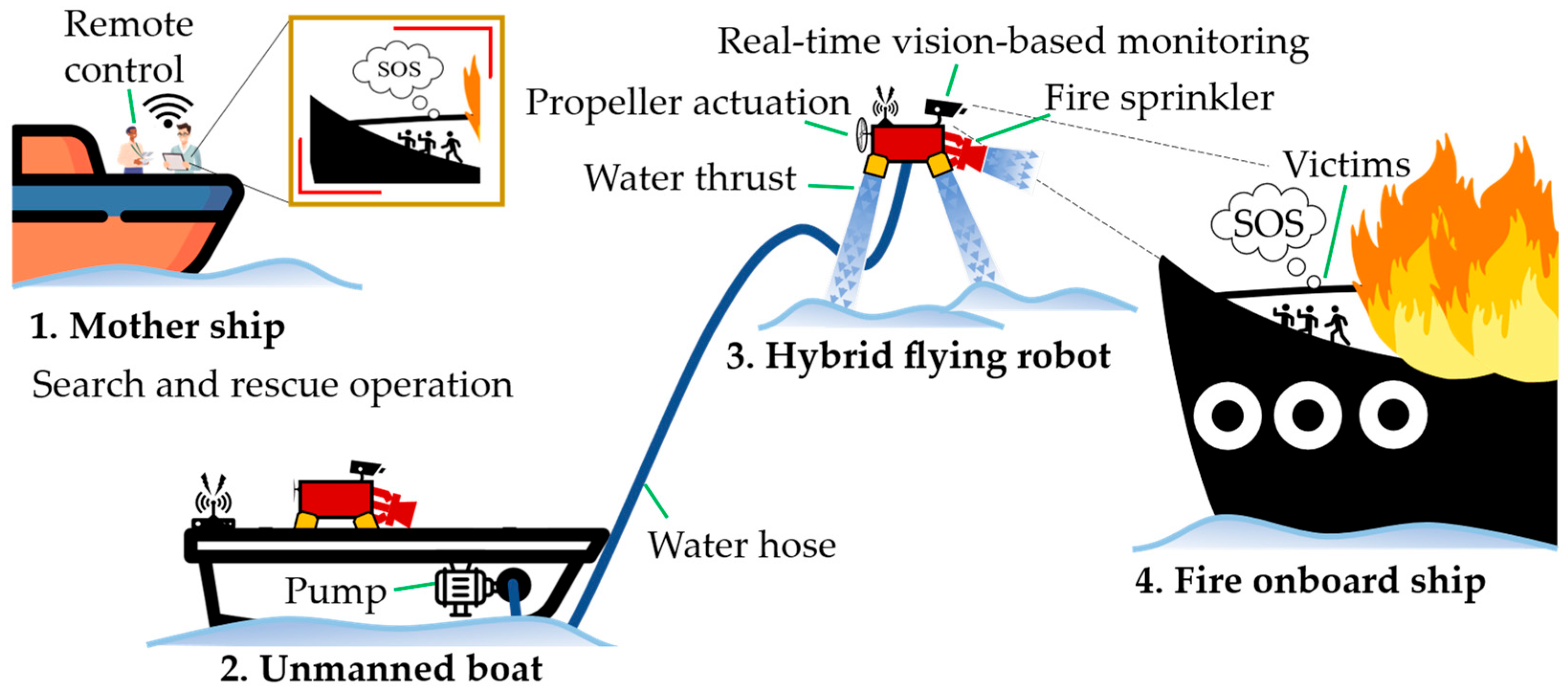
To address the limitations mentioned, this paper proposes a novel water-powered flying robot equipped with aerial propellers and designs a state feedback control scheme to govern its movement. Specifically, four propellers are horizontally positioned on top of the flying robot. This configuration utilizes the air thrust generated by the propellers to produce the actuating forces and torques required for robot motion. By using lightweight propeller modules, this approach overcomes the issues of unnecessary increases in the overall mass of the robot and the non-minimum phase phenomenon, while maintaining the simplicity of the overall system design. The most important aspect of the proposed design is its universal applicability. The propeller mechanism can be integrated with any existing water-powered flying robot without requiring major modifications to the original system. The target application scenario of the system is illustrated in Figure 1. Particularly, by integrating advanced equipment, e.g., camera systems and water sprinklers, the robot is capable of performing firefighting and search-and-rescue missions.

In summary, the contributions of this study can be outlined as follows:

• A novel conceptual design of the water-powered flying robot equipped with propellers is proposed.
• A mathematical model of this proposed system is formulated to reflect its dynamical characteristics.
• Full-state feedback designed based on a linear matrix inequality (LMI) approach is developed, incorporating an integral action control law and a control allocation method to fulfill the stability and tracking performance of the system.
• Comparative simulation studies are conducted to evaluate and validate the feasibility of the proposed flying robot.

The rest of the paper is written as follows. Section 2 introduces the conceptual design of the proposed flying robot, analyzes the robot configuration, and derives its mathematical model. In Section 3, the control system designs are conducted. Section 4 comprehensively overviews the simulation setup and the resulting findings. Finally, the conclusions are outlined in Section 5.

2. Conceptual Design and System Modeling

In this section, the conceptual design and mathematical model for the proposed flying robot are presented, highlighting the key equations and dynamics that govern their behavior. This model provides the foundation for understanding the control strategies employed in the system.

2.1. Conceptual Design of the Flying Robot

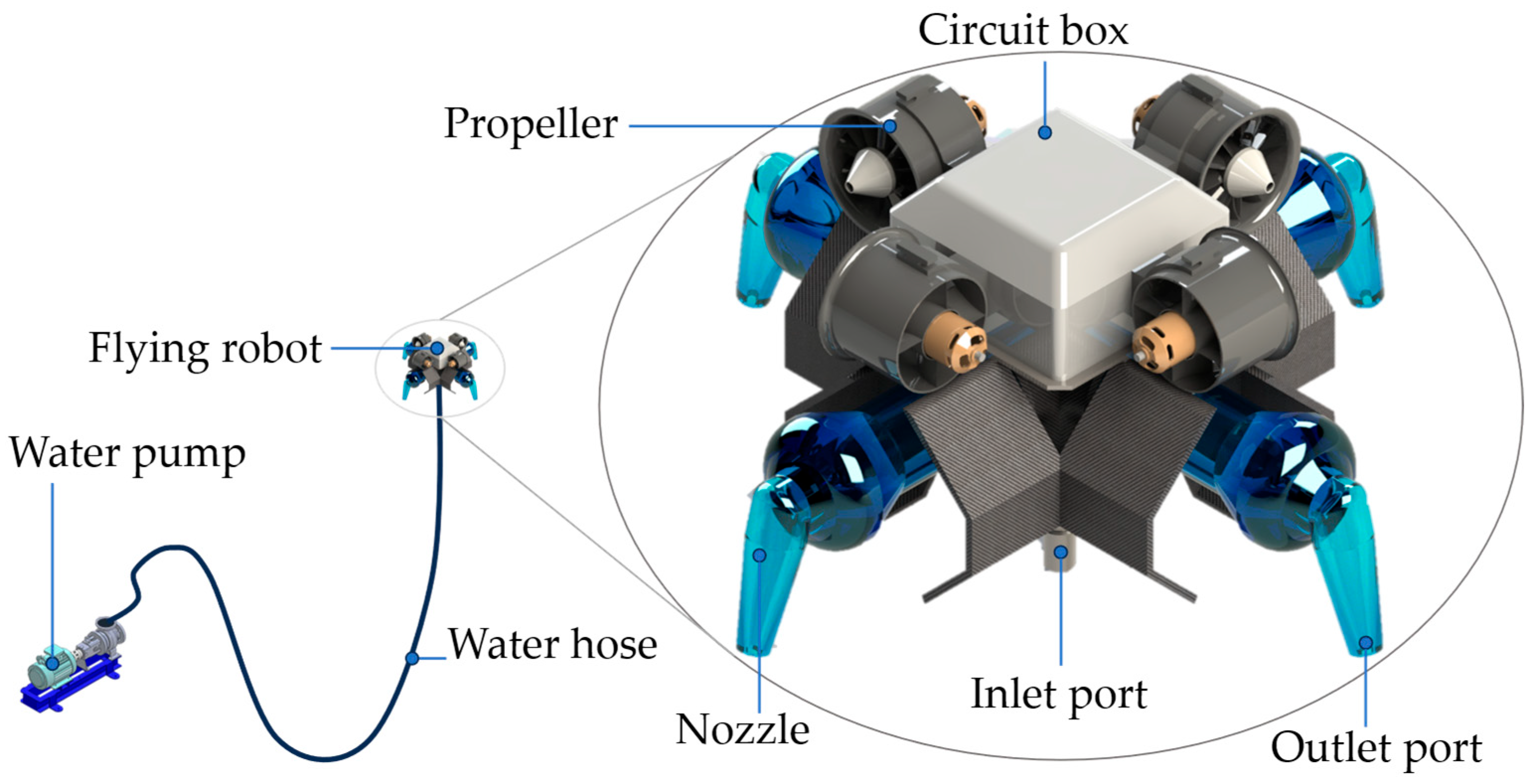
This study proposes a flying robot designed to operate in and around aquatic environments, allowing it to carry out various tasks such as firefighting, assisting marine towing operations, and more. The structural design of this system consists of three main components: a water pump, a water hose, and a flying robot. The overall structure of the system is depicted in Figure 2.

The water pump can be positioned either on the ground or on a floating platform, depending on the location of the available water source. High-pressure water is forced through a hose connected from the pump to the input port of the robot, where it is expelled through four downward-facing nozzles. As water is expelled downward at high speed, an equal and opposite reaction force pushes the robot upward. The cross-sectional area of the nozzle outlet is significantly smaller than that of the water inlet port of the robot, allowing the pressurized water to accelerate as it exits. Furthermore, the flow rate of the water pump is actively controlled to enable precise altitude adjustments of the flying robot.

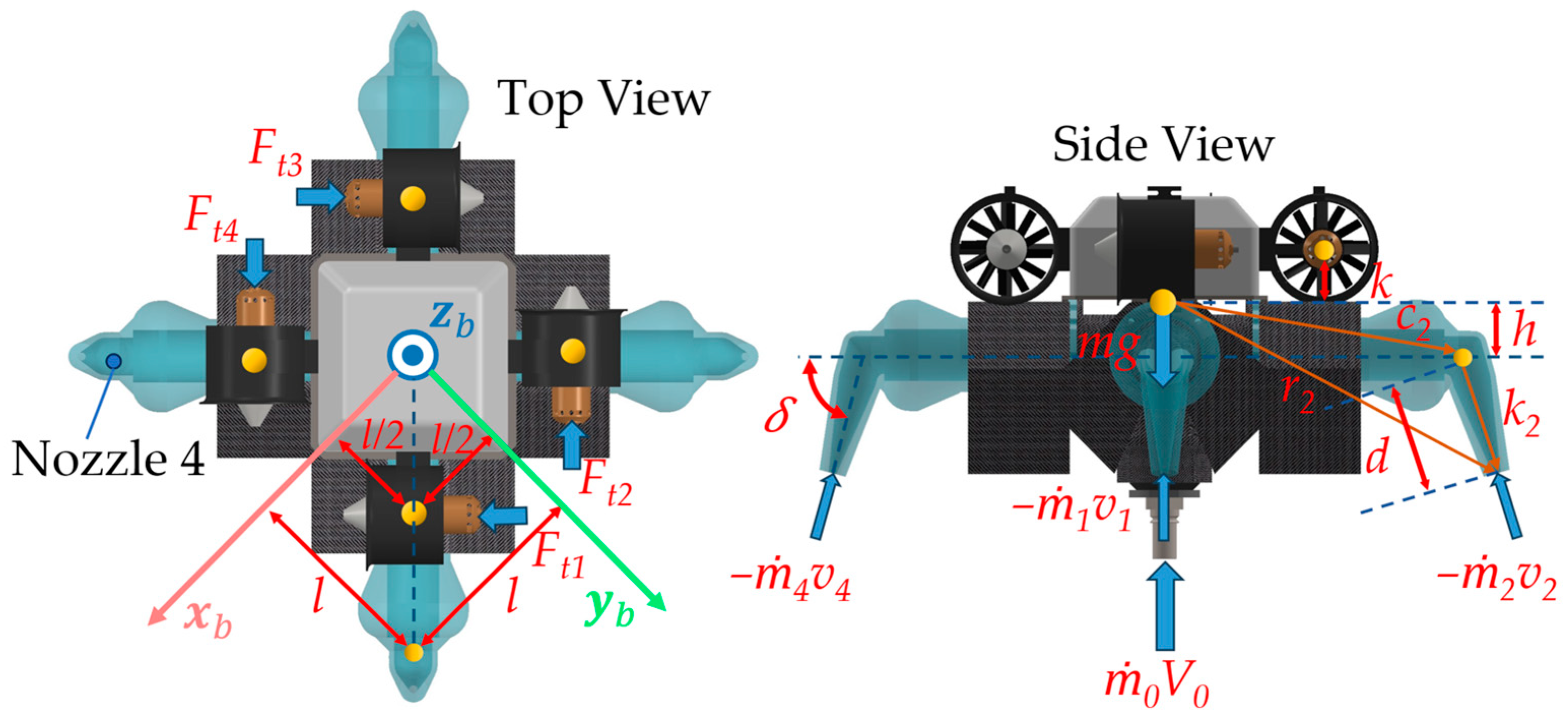
The proposed flying robot is equipped with four fixed nozzles and four propellers. The nozzles spray high-speed water jets to generate thrust. All four nozzles are directed downward, producing thrust in the vertical direction. They are arranged symmetrically around the robot’s vertical axis, spaced at 90-degree intervals. Each pair of opposing nozzles is aligned symmetrically across the central plane. This configuration effectively cancels out horizontal forces and moments. As a result, the thrust primarily contributes to vertical lift while minimizing unintended rotational or translational motion in the horizontal plane.

In addition, to supply the remaining forces and moments required for full control of 6-DOF, four horizontally oriented propellers are evenly distributed around the robot, generating airflow parallel to the horizontal plane. This design helps overcome limitations commonly encountered in traditional drone designs, particularly in achieving stable horizontal motion and rotational control. Each propeller operates in a fixed rotational direction, generating a thrust force $F_{ti} (i=1~4),$ as shown in Figure 3. In this configuration, each pair of opposing propellers generates two opposite forces, while each pair of adjacent propellers produces two perpendicular (orthogonal) forces. By integrating this propeller configuration with controlled flow rate regulation from the water pump, the robot is capable of producing the necessary forces and moments across all axes. Therefore, precise maneuvering and robust attitude stabilization are more easily achieved.

Moreover, unlike conventional quadrotors or drones, where horizontal motion is achieved subsequently through angular tilting and rolling, the propellers in this system can directly generate horizontal forces. This unique feature is expected to provide enhanced controllability for movement. By adjusting the water mass flow rate of the pump and the thrust forces generated by the propellers, the proposed system can achieve full flight in the air.

2.2. Kinematics Analysis

To derive the characteristics of the proposed robot in the air, two Cartesian coordinate systems, i.e., the body-fixed frame $O_b{x}_b{y}_b{z}_b$ and Earth reference frame $Oxyz$, are used, as depicted in Figure 4, in which the body-fixed frame has its origin placed at the mass center of the robot and its $x_b-$, $y_b-$, and $z_b-$ axes point along forward, leftward, and upward directions, respectively. We assume that the mass center is also the centroid of the robot, for the sake of simplicity. The latter coordinates follow the east, north, and up directions, respectively. Moreover, the kinematic relationship between the two coordinates can be described via the following transformation matrices:

$$\left[\begin{array}{c}\dot{x}\\ \dot{\phi }\end{array}\right]=\left[\begin{array}{cc}{R}_b^E& O_3\\ O_3& T_b^E\end{array}\right]\left[\begin{array}{c}{\dot{x}}_b\\ {\dot{\phi }}_b\end{array}\right]$$

(1)

where $\dot{x}={\left[\begin{array}{ccc}\dot{x}& \dot{y}& \dot{z}\end{array}\right]}^T$ and ${\dot{x}}_b={\left[\begin{array}{ccc}{\dot{x}}_b& {\dot{y}}_b& {\dot{z}}_b\end{array}\right]}^T$ are the state vectors. $R_b^E$ is the rotation matrix of the former $\left(O_b{x}_b{y}_b{z}_b\right)$ relative to the latter $\left(Oxyz\right)$. ${\dot{\phi }}_b={\left[\begin{array}{ccc}{\dot{\varphi }}_b& {\dot{\theta }}_b& {\dot{\psi }}_b\end{array}\right]}^T$ is the rotation rate of the body-fixed frame and $\dot{\phi }={\left[\begin{array}{ccc}\dot{\varphi }& \dot{\theta }& \dot{\psi }\end{array}\right]}^T$ is the rate vector of the three Euler angles describing the orientation of this frame relative to the reference frame. $T_b^E$ is the transformation matrix between them [22]. Moreover, $O_3$ is a 3-by-3 zero matrix.

2.3. Dynamics Analysis

The dynamics of the proposed flying robot are described by the Newton–Euler equations, that is:

$$\left[\begin{array}{cc}m{I}_3& O_3\\ O_3& J\end{array}\right]\left[\begin{array}{c}{\ddot{x}}_b\\ {\ddot{\phi }}_b\end{array}\right]+\left[\begin{array}{c}{\dot{\phi }}_b\times {\dot{x}}_b\\ {\dot{\phi }}_b\times J{\dot{\phi }}_b\end{array}\right]=\left[\begin{array}{c}{F}_b\\ {\tau }_b\end{array}\right]$$

(2)

where $I_3$ represents the identity matrix of size three, m is the mass of the flying robot with its contained water, and $J=diag\left\{J_{bx}, J_{by}, J_{bz}\right\}$ is its inertia matrix, assuming that it is diagonal. Moreover, $F_b$ and ${\tau }_b$ represent forces and torques acting on the robot and can be interpreted as follows:

$$\begin{array}{c}{F}_b=F_p+F_n+m{\left(R_b^E\right)}^{T}g+{\left[0 0 {\dot{m}}_0{V}_0+PA\right]}^T+d_F\\ {\tau }_b={\tau }_p+{\tau }_n+d_{\tau }\end{array}$$

(3)

In the above equation, $F_p$ is the vector of the actuating forces generated by the propeller’s thrust, and ${\tau }_p$ represents their resultant torques. $F_n$ and ${\tau }_n$ contain the forces and torque, respectively, generated by the water thrust. Additionally, $g={\left[0 0 -g\right]}^T$ is the gravitational acceleration vector observed from the reference frame, with $g$ the gravitational acceleration. $\left({\dot{m}}_0{V}_0+PA\right)$ is the vertical force created by the inlet water flow and pressure, where ${\dot{m}}_0$ is its mass flow rate through the inlet port, $V_0={\dot{m}}_0{\left(\rho A\right)}^{-1}$, with $\rho$ the water density and A the inlet’s cross-sectional areas, is the axial velocity of the water flow, and P is the supplying pressure created by the pump. Finally, $d_F$ and $d_{\tau }$ are the remaining unmodeled terms, including wind gust, ground effect, and water hose effect.

Accordingly, $F_p$ and ${\tau }_p$ relate to each propeller thrust as follows:

$$F_p={\displaystyle \sum _{i=1}^4{F}_{pi}}={\displaystyle \frac{\sqrt{2}}{2}}\left[\begin{array}{c}{F}_{t1}-F_{t2}-F_{t3}+F_{t4}\\ -F_{t1}-F_{t2}+F_{t3}+F_{t4}\\ 0\end{array}\right], {\tau }_p={\displaystyle \sum _{i=1}^4{p}_i\times F_{pi}}={\displaystyle \frac{\sqrt{2}}{2}}\left[\begin{array}{c}k\left(-F_{t1}-F_{t2}+F_{t3}+F_{t4}\right)\\ k\left(F_{t1}-F_{t2}-F_{t3}+F_{t4}\right)\\ l\left(-F_{t1}+F_{t2}-F_{t3}+F_{t4}\right)\end{array}\right]$$

(4)

where the position of the ith propeller ($p_i$) is determined as follows:

$$p_i={\left[{(-1)}^{(i-1)(i-4)/2}{\displaystyle \frac{l}{2}}{(-1)}^{(i-1)(i-2)/2}{\displaystyle \frac{l}{2}}k\right]}^T, i=1\sim 4$$

(5)

with k is the distance between the propeller’s center of gravity and the robot’s $O_b{x}_b{y}_b$ plane with respect to the $z_b$–axis.

In a similar manner, the outlet position of each nozzle is defined as follows:

$$\begin{array}{c}{ r}_i=c_i+k_i, c_i={\left[\begin{array}{c}{(-1)}^{(i-1)(i-4)/2}l{(-1)}^{(i-1)(i-2)/2}l-h\end{array}\right]}^T\\ k_i=R_i{\left[\begin{array}{ccc}0& d& 0\end{array}\right]}^T, R_i=R_{\beta }^{z_b}{R}_{-\delta }^{x_b}, \beta =-0.75\pi +0.5\pi i\end{array}$$

(6)

where vectors $c_i$ and $k_i$ describe the position of the center of the rotation of the ith $\left(i=1~4\right)$ nozzle and the part of the nozzle’s rotation with a length of d, respectively. In which, $R_{-\delta }^{x_b}$ and $R_{\beta }^{z_b}$ denote the rotation matrices of the rotations $\delta$ and β about the corresponding $x_b$–axis and $z_b$–axis, respectively. Then, $F_n$ and ${\tau }_n$ are rewritten in terms of the forces at the nozzle outlets as follows:

$$\begin{array}{c}{F}_n={\displaystyle \sum _{i=1}^4{F}_{ni}}=\left[\begin{array}{c}\cos \delta \left(F_{n1}-F_{n2}-F_{n3}+F_{n4}\right)\\ \cos \delta \left(F_{n1}+F_{n2}-F_{n3}-F_{n4}\right)\\ \sin \delta \left(F_{n1}+F_{n2}+F_{n3}+F_{n4}\right)\end{array}\right], {\tau }_n={\displaystyle \sum _{i=1}^4{r}_i\times F_{ni}}=\sigma \left[\begin{array}{c}{F}_{n1}+F_{n2}-F_{n3}-F_{n4}\\ -F_{n1}+F_{n2}-F_{n3}+F_{n4}\\ 0\end{array}\right],\\ \sigma =l+{\displaystyle \frac{\sqrt{2}d\cos \left(\delta \right)}{2}}+h+d\sin \left(\delta \right)\end{array}$$

(7)

since $F_{n1}=F_{n2}=F_{n3}=F_{n4}$, the force and torque of the water thrust can be written as follows:

$$F_n={\displaystyle \sum _{i=1}^4{F}_{ni}}=\left[\begin{array}{c}0\\ 0\\ 4F_{ni}\sin \delta \end{array}\right], {\tau }_p=0$$

(8)

The proof of the equality of the forces generated by the nozzle is provided in the Section 2.4.

2.4. Actuator Modeling

The thrust generated by the propellers can be written as follows:

$$F_{ti}=\varsigma {\Omega }_i^2\mathrm{sgn}(\Omega )$$

(9)

with $\varsigma$ the propeller’s thrust coefficient depending on the design of the propeller, and $\Omega$ being the propeller’s rotation velocity, and $\mathrm{sgn}(•)$ the signum function of the corresponding $(•)$. As shown in Equation (9), the generated thrust is proportional to the square of the velocity. Therefore, controlling the propeller’s rotational velocity is effectively equivalent to controlling the generated thrust.

Remark 1.

The direction of propeller rotation determines the direction of thrust. In the case of a unidirectional propeller, which rotates in a pre-defined direction, the resulting thrust is constrained to be non-negative.

In order to model the water force generated at each nozzle outlet ($F_{ni}$), let us adopt the following popular assumption:

Assumption 1.

The water volume is frictionless and steady [23].

Assumption 2.

The body distributor and its contained water volume are not deformable.

Assumption 3.

The water mass flow rate of the water outlet ports is equal to each other and to fourth of the water mass flow rate of the water inlet port.

Furthermore, the relative velocity of the jetted water at the nozzle’s outlet, ${\overline{v}}_i$, is derived similarly to $k_i$, and the absolute velocity of the jetted water $v_i$ is therefore interpreted as the following:

$$v_i={\overline{v}}_i+v_b, {\overline{v}}_i=R_i{\left[0 V_i 0\right]}^T$$

(10)

where $V_i$ represents the axial velocity of the water flowing out at the ith nozzle’s outlet.

Under Assumption 2, the water-induced thrust forces of each nozzle can be obtained from the differential linear momentum equation for incompressible flow, as follows:

$$F_{ni}=-{\displaystyle \frac{{\dot{m}}_i^2}{a\rho }}\left[\begin{array}{c}-\cos \left(\delta \right)\sin \left(\beta \right)\\ \cos \left(\delta \right)\cos \left(\beta \right)\\ -\sin \left(\delta \right)\end{array}\right]+\left(-{\dot{m}}_i\right)\left(v_b+{\dot{\phi }}_b\times r_i\right)$$

(11)

where

• ${\dot{m}}_i={\dot{m}}_0/4$ (Assumption 3): Mass flow rates at the water outlet ports.
• a: Cross-sectional areas of water outlet ports.

Given that the velocity of the water jet expelled from the nozzles is significantly greater than the velocity of the robot itself, the resulting water force can be reasonably approximated by the following expression:

$$F_{ni}\approx -{\displaystyle \frac{{\dot{m}}_i^2}{a\rho }}\left[\begin{array}{c}-\cos \left(\delta \right)\sin \left(\beta \right)\\ \cos \left(\delta \right)\cos \left(\beta \right)\\ -\sin \left(\delta \right)\end{array}\right]$$

(12)

Hence, the thrust force at the ith nozzle outlet is a function of the mass flow rate through the ith nozzle and the mentioned Assumption 3, so the resulting water thrust forces from all nozzles are equal.

By substituting (8), (5) into (3), (3) into (2), and using the kinematic relationship (1), the translational and rotational dynamics of the flying robot in the Earth-fixed frame can be obtained as follows:

$$\ddot{x}=R_b^E{C}_{x}U+F_x, \ddot{\phi }=T_b^E{C}_{\phi }U+F_{\phi }$$

(13)

Here, the control input is identified as follows:

$$\begin{array}{c}U={\left[\begin{array}{cccc}\Delta F_x& \Delta F_y& \Delta F_{\psi }& {{\dot{m}}_0}^2\end{array}\right]}^T , \\ \Delta F_x=F_{t1}-F_{t2}-F_{t3}+F_{t4}, \Delta F_y=-F_{t1}-F_{t2}+F_{t3}+F_{t4}, \Delta F_{\psi }=-F_{t1}+F_{t2}-F_{t3}+F_{t4}\end{array}$$

(14)

and the term $C_x$ and $C_{\phi }$ are obtained as follows:

$$\begin{array}{c}{C}_x=\left[\begin{array}{cccc}{c}_1& 0& 0& 0\\ 0& c_1& 0& 0\\ 0& 0& 0& c_2\end{array}\right], C_{\phi }=\left[\begin{array}{cccc}0& -c_3& 0& 0\\ c_4& 0& 0& 0\\ 0& 0& c_5& 0\end{array}\right], \\ c_1={\displaystyle \frac{\sqrt{2}}{2m}}, c_2={\displaystyle \frac{\sin \left(\delta \right)}{4ma\rho }}+{\displaystyle \frac{1}{mA\rho }}, c_3={\displaystyle \frac{\sqrt{2}k}{2J_{bx}}}, c_4={\displaystyle \frac{\sqrt{2}k}{2J_{by}}}, c_5={\displaystyle \frac{\sqrt{2}l}{2J_{bz}}}\end{array}$$

(15)

Beyond that, the matrices $F_x$ and $F_{\phi }$ are internal dynamics of the system and are expressed as follows:

$$\begin{array}{c}{F}_x=E\dot{x}+R_b^{E}F{\left(T_b^E\right)}^{-1}\dot{\phi }+g+F_{dx},\\ F_{\phi }=T_b^{E}M{\left(R_b^E\right)}^T\dot{x}+N\dot{\phi }+F_{d\phi }\end{array}$$

(16)

where the matrices E, F, M, and N in Equation (16) are expanded as follows:

$$\begin{array}{c}E=-{\displaystyle \frac{{\dot{m}}_0}{m}}diag\left\{1, 1, 1\right\}, F={\displaystyle \frac{{\dot{m}}_0{\sigma }_1}{m}}\left[\begin{array}{ccc}0& 1& 0\\ 1& 0& 0\\ 0& 0& 0\end{array}\right],\\ M=\left[\begin{array}{ccc}0& -{\displaystyle \frac{{\dot{m}}_0{\sigma }_1}{J_{bx}}}& 0\\ {\displaystyle \frac{{\dot{m}}_0{\sigma }_1}{J_{by}}}& 0& 0\\ 0& 0& 0\end{array}\right], N=-\left[\begin{array}{ccc}{\displaystyle \frac{{\dot{m}}_0{\sigma }_3}{J_{bx}}}& 0& 0\\ 0& {\displaystyle \frac{{\dot{m}}_0{\sigma }_3}{J_{by}}}& 0\\ 0& 0& {\displaystyle \frac{2{\dot{m}}_0{{\sigma }_2}^2}{J_{bz}}}\end{array}\right]\end{array}$$

(17)

with:

$${\sigma }_1=h+d\sin \left(\delta \right), {\sigma }_2=l+{\displaystyle \frac{\sqrt{2}d\cos \left(\delta \right)}{2}}, {\sigma }_3={{\sigma }_1}^2+{{\sigma }_2}^2$$

(18)

For completeness, $F_{dx}$ and $F_{d\phi }$ represent the remaining terms after substitution; they include input–output coupling terms, higher-order nonlinearities, and external disturbances.

In addition, the derived dynamic equations of the proposed flying robot reveal several distinctive features, which are outlined in the following remarks.

Remark 2.

The system itself exhibits nonlinear dynamics.

Remark 3.

With five actuators controlling six degrees of freedom, the system is underactuated.

Remark 4.

The water pump generates purely vertical thrust for lift, while the propellers solely produce horizontal thrust and the corresponding torques. This configuration enables independent actuation between the two propulsion sources.

Remark 5.

Coupling exists between the translational motions in the x and y directions and the rotational motions in roll and pitch. However, thanks to the incorporation of a novel actuator, the system successfully decouples the horizontal actuation from the water thrust. As a result, the robot achieves enhanced maneuverability and greater operational flexibility.

3. Control System Design

For this study, the control strategies are implemented to evaluate the performance of the proposed actuation system. To achieve this objective, two effective control strategies are utilized for flying robots. These include state feedback control and PID control, applied to the general tasks of stabilization and trajectory tracking. Each method offers unique advantages for various aspects of the control system. When integrated effectively, they can provide a robust and reliable solution for the trajectory tracking problem.

3.1. PID Controller Design

Given a desired trajectory for the flying robot, the PID controller processes the error between the desired and actual response of the flying robot. Based on that, it can generate control inputs that minimize this error over time. Figure 5 depicts the control scheme for this controller.

In Equations (13) and (16), let $F_{PID}$ represent the controllable forces and torques for the 6-degree-of-freedom motion. That is:

$$\left[\begin{array}{c}\ddot{x}\\ \ddot{\phi }\end{array}\right]=F_{PID}+\left[\begin{array}{l}g\\ O_{3\times 1}\end{array}\right]+\left[\begin{array}{l}E\dot{x}+R_b^{E}F{\left(T_b^E\right)}^{-1}\dot{\phi }+F_{dx}\\ T_b^{E}M{\left(R_b^E\right)}^T\dot{x}+N\dot{\phi }+F_{d\phi }\end{array}\right], \mathrm{with} F_{PID}=\left[\begin{array}{c}{R}_b^E{C}_x\\ T_b^E{C}_{\phi }\end{array}\right]U$$

(19)

Let us define the desired reference, including both translational motion $x_d={\left[\begin{array}{ccc}{x}_d& y_d& z_d\end{array}\right]}^T$ and orientation ${\phi }_d={\left[\begin{array}{ccc}{\varphi }_d& {\theta }_d& {\psi }_d\end{array}\right]}^T$, in which the roll and pitch reference angles are zero to reflect the requirement of a stable flight motion. Then, the tracking error can be expressed as $e={\left[\begin{array}{cc}{x_d}^T-x^T& {{\phi }_d}^T-{\phi }^T\end{array}\right]}^T$. Following that, the PID control law for this system is formulated as follows:

$$F_{PID}=K_{P}e+K_I{\displaystyle \underset{0}{\overset{t}{\int }}e(t)dt+K_D\dot{e}-\left[\begin{array}{c}g\\ O_{3\times 1}\end{array}\right]}$$

(20)

with $K_P, K_I \mathrm{and} K_D$ representing the controller’s gains, which are selected to ensure the stability of the control system. Gravitational acceleration is also incorporated into the control law. The PID law computes the forces and torques required for the motion in each direction.

Then, from the definition of $F_{PID}$, the control input U is obtained as follows:

$$U=R_m{F}_{PID}, C_m=\left[\begin{array}{c}{C}_x\\ C_{\phi }\end{array}\right], R_m={C_m}^{†}\left[\begin{array}{cc}{\left(R_b^E\right)}^{-1}& 0\\ 0& {\left(T_b^E\right)}^{-1}\end{array}\right]$$

(21)

The term ${C_m}^{†}$ denotes the pseudo-inverse of $C_m$, which is a generalized inverse that can be computed even for non-square or rank-deficient matrices.

3.2. State Feedback Controller Design with Linear Matrix Inequality

The primary objective of designing a state feedback controller using linear matrix inequalities (LMIs) is to achieve robust and stable control performance for dynamic systems, particularly for the proposed flying robot, which exhibits nonlinear dynamics and is subject to external disturbances. To come up with the control law, the flying robot’s dynamics is transformed into the Earth reference frame using the kinematic relationship (1), which is expressed as Equation (10). Then, the dynamics of the proposed flying robot can be linearized with respect to the specified state variables, control inputs, and system outputs as detailed below:

$$\begin{array}{c}X={\left[x y z-\overline{z} \varphi \theta \psi \dot{x} \dot{y} \dot{z} \dot{\varphi } \dot{\theta } \dot{\psi }\right]}^T,\\ Y={\left[\begin{array}{cccc}x& y& z-z_0& \psi \end{array}\right]}^T, \\ \overline{U}={\left[\begin{array}{cccc}\Delta F_x& \Delta F_y& \Delta F_{\psi }& {\dot{m}}_0-{\dot{\overline{m}}}_0\end{array}\right]}^T\end{array}$$

(22)

The system is then linearized around a local equilibrium point, where the flying robot is stabilized at the desired altitude $\overline{z}$ with an appropriate constant mass flow rate ${\dot{\overline{m}}}_0$ to maintain flight at this position. At this equilibrium, the horizontal and rotational motions are zero, and the propellers are considered inactive. Based on these conditions, let us define the local equilibrium point as follows:

$$X_0={\left[\begin{array}{ccc}{O}_{1\times 2}& \overline{z}& O_{1\times 9}\end{array}\right]}^T, U_0={\left[\begin{array}{cccc}0& 0& 0& {\dot{\overline{m}}}_0\end{array}\right]}^T$$

(23)

The standard linear state-space form of the system is obtained as follows:

$$\dot{X}=AX+B\overline{U}+D, Y=CX$$

(24)

in which matrices A and B are obtained by Lyapunov’s linearization method, and C is the output matrix; these matrices are presented as below:

$$A=\left[\begin{array}{cc}{O}_6& I_6\\ O_{6\times 3}& \begin{array}{ccccccccc}0& a_5& 0& a_1& 0& 0& 0& {\displaystyle \frac{a_2}{m}}& 0\\ -a_5& 0& 0& 0& a_1& 0& {\displaystyle \frac{-a_2}{m}}& 0& 0\\ 0& 0& 0& 0& 0& a_1& 0& 0& 0\\ 0& 0& 0& 0& {\displaystyle \frac{-a_2}{J_{bx}}}& 0& {\displaystyle \frac{a_3}{J_{bx}}}& 0& 0\\ 0& 0& 0& {\displaystyle \frac{a_2}{J_{by}}}& 0& 0& 0& {\displaystyle \frac{a_3}{J_{by}}}& 0\\ 0& 0& 0& 0& 0& 0& 0& 0& {\displaystyle \frac{a_4}{J_{bz}}}\end{array}\end{array}\right], \begin{array}{c}\begin{array}{l}B=\left[\begin{array}{c}{O}_{6\times 4}\\ \begin{array}{cccc}{b}_1& 0& 0& 0\\ 0& b_1& 0& 0\\ 0& 0& 0& b_2\\ 0& -b_3& 0& 0\\ b_4& 0& 0& 0\\ 0& 0& b_5& 0\end{array}\end{array}\right]\\ \end{array}\\ C=\left[\begin{array}{c}\begin{array}{cc}{I}_3& O_{3\times 9}\end{array}\\ \begin{array}{ccc}{O}_{1\times 5}& 1& O_{1\times 6}\end{array}\end{array}\right]\end{array}$$

(25)

with:

$$\begin{array}{c}{a}_1={\displaystyle \frac{-{\dot{\overline{m}}}_0}{m}}, a_2={\dot{\overline{m}}}_0\left[h+d\sin \left(\delta \right)\right], a_3=-{\dot{\overline{m}}}_0\left\{4{\left[h+d\sin \left(\delta \right)\right]}^2+4{\left[l+{\displaystyle \frac{\sqrt{2}}{2}}d\cos \left(\delta \right)\right]}^2\right\},\\ a_4=-2{\dot{\overline{m}}}_0{\left[l+{\displaystyle \frac{\sqrt{2}}{2}}d\cos \left(\delta \right)\right]}^2, a_5={\displaystyle \frac{{{\dot{\overline{m}}}_0}^2\sin \left(\delta \right)}{4m\rho a}}, b_1={\displaystyle \frac{\sqrt{2}}{2m}}, b_2=2{\dot{\overline{m}}}_0\left({\displaystyle \frac{\sin \left(\delta \right)}{4ma\rho }}+{\displaystyle \frac{1}{mA\rho }}\right),\\ b_3={\displaystyle \frac{\sqrt{2}k}{2J_{bx}}}, b_4={\displaystyle \frac{\sqrt{2}k}{2J_{by}}}, b_5={\displaystyle \frac{\sqrt{2}l}{2J_{bz}}}\end{array}$$

(26)

Lastly, vector $D$ represents the remaining nonlinear elements and disturbances.

In order to derive a robust state feedback control for the flying robot, let us take into consideration an integral action of the tracking error. That is, the system with its state variables defined by tracking errors is as follows:

$$\begin{array}{c}\dot{\tilde{X}}=\tilde{A}\tilde{X}+\tilde{B}\overline{U}+B_d\tilde{D},\\ \tilde{Y}=\tilde{C}\tilde{X}\end{array}$$

(27)

with augmented matrices as follows:

$$\begin{array}{c}\tilde{X}={\left[\begin{array}{cc}{\xi }^T& e^T\end{array}\right]}^T, \tilde{Y}={\left[\begin{array}{cccc}-\varphi & -\theta & {\dot{\epsilon }}^T& e^T\end{array}\right]}^T, \tilde{A}=\left[\begin{array}{cc}-A& O_{12\times 4}\\ C& O_4\end{array}\right], \tilde{B}=\left[\begin{array}{c}-B\\ O_4\end{array}\right],B_d=\left[\begin{array}{c}{O}_{6\times 10}\\ I_{10}\end{array}\right], \\ \tilde{C}=\left[\begin{array}{c}\begin{array}{ccc}{O}_{2\times 3}& I_2& O_{2\times 11}\end{array}\\ \begin{array}{cc}{O}_{10\times 6}& I_{10}\end{array}\end{array}\right], \epsilon ={\left[\begin{array}{cccccc}{x}_d-x& y_d-x& z_d-z& -\varphi & -\theta & {\psi }_d-\psi \end{array}\right]}^T , \xi =\left[\begin{array}{c}\epsilon \\ \dot{\epsilon }\end{array}\right]\\ \dot{e}={\left[\begin{array}{cccc}{x}_d-x& y_d-y& z_d-z& {\psi }_d-\psi \end{array}\right]}^T\end{array}$$

(28)

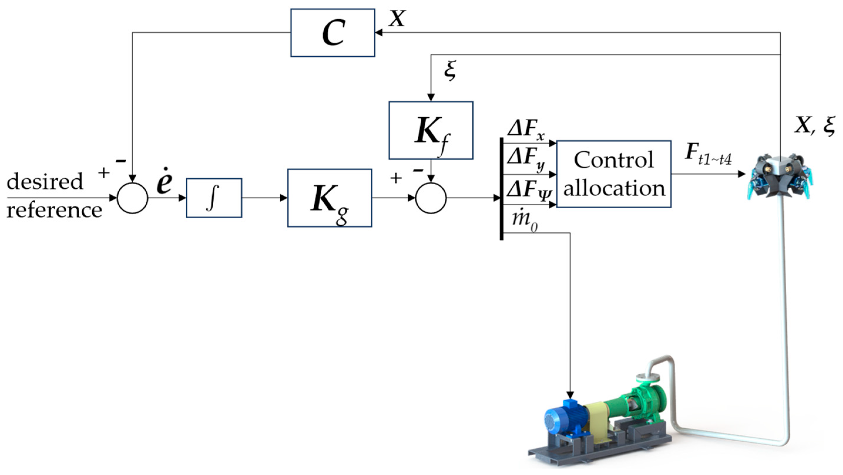
Based on the linear state feedback, the control law is proposed in the form:

$$\overline{U}=K\tilde{X}=-K_f\xi +K_{g}e, K=\left[\begin{array}{cc}-K_f& K_g\end{array}\right]$$

(29)

The schematic representation of this control strategy is illustrated in Figure 6. To analyze the stability conditions of the closed-loop control system, let us define a Lyapunov function candidate as follows:

$$V={\tilde{X}}^{T}P\tilde{X}$$

(30)

where P is a 16-by-16 positive definite and symmetrical matrix. The time derivative of the Lyapunov function candidate is obtained as follows:

$$\dot{V}={\tilde{X}}^T\left({\tilde{A}}^{T}P+K^T{\tilde{B}}^{T}P+P\tilde{A}+P\tilde{B}K\right)\tilde{X} +{\tilde{X}}^{T}P{B}_d\tilde{D}+{\tilde{D}}^T{B_d}^{T}P\tilde{X}$$

(31)

Given a $\gamma >0$, let us consider the following inequality:

$$\dot{V}+{\tilde{Y}}^T\tilde{Y}-{\gamma }^2{\tilde{D}}^T\tilde{D}\le 0$$

(32)

This inequality can be rewritten in the form of a matrix inequality as follows [24]:

$$\left[\begin{array}{cc}{\tilde{A}}^{T}P+K^T{\tilde{B}}^{T}P+P\tilde{A}+P\tilde{B}K+C^{T}C& P{B}_d\\ B_d^{T}P& -{\gamma }^{2}I\end{array}\right]\le 0$$

(33)

This is a bilinear matrix inequality that is difficult to solve. By denoting $Q=P^{-1}$ and $Z=KQ$, Equation (33) is equivalent to the following linear matrix inequality [24]:

$$\left[\begin{array}{ccc}Q{\tilde{A}}^T+\tilde{A}Q+Z^T{\tilde{B}}^T+\tilde{B}Z& B_d& Q{\tilde{C}}^T\\ B_d^T& -\gamma I_{10}& O_{10\times 12}\\ \tilde{C}Q& O_{12\times 10}& -\gamma I_{12}\end{array}\right]\le 0$$

(34)

One can see that if there exist Q and Z such that Equation (34) holds, it implies ${\tilde{Y}}^T\tilde{Y}-{\gamma }^2{\tilde{D}}^T\tilde{D}\le 0$. This inequality results in $L_2:=\underset{{‖\tilde{D}‖}_2\ne 0}{\sup }\left({\displaystyle \raisebox{1ex}{${‖\tilde{Y}‖}_2$}\!\left/ \!\raisebox{-1ex}{${‖\tilde{D}‖}_2$}\right.}\right)\le \gamma$, where $L_2$ denotes the $L_2$ gain, i.e., $H_{\infty }$ norm, of the system [21]. Minimizing $\gamma$ over the variables Z and Q results in the smallest upper bound on the $L_2$ gain of the system. Then, the optimal feedback gain K is derived.

3.3. Control Allocation Design

In the proposed control system, the control inputs $\Delta F_x$, $\Delta F_y$, and $\Delta F_{\psi }$ are analyzed to compute the corresponding input values $F_{t1}, F_{t2}, F_{t3},$ and $F_{t4}$. From Equation (14), the system of equations has fewer equations than unknowns, the coefficient matrix has full row rank (rank 3), and the system is always consistent. Therefore, the system of equations has infinitely many solutions for any real values of $\Delta F_x$, $\Delta F_y$, and $\Delta F_{\psi }$. Furthermore, the flying robot employs a unidirectionally rotating propeller, which inherently produces thrust in a single, positive direction. This section presents the methodology employed to address this problem.

Initially, by sequentially combining the equations of the element $\Delta F_x$, $\Delta F_y$, and $\Delta F_{\psi }$ in Equation (14), the following result is obtained:

$$\left\{\begin{array}{c}2F_{t1}=-\Delta F_{\psi }-\Delta F_y+2F_{t4}\\ 2F_{t2}=-\Delta F_x-\Delta F_y+2F_{t4}\\ 2F_{t3}=-\Delta F_x-\Delta F_{\psi }+2F_{t4}\end{array}\right.$$

(35)

From Equation (35), the requirement of the propellers’ force being positive can be achieved by:

$$\left\{\begin{array}{c}2F_{t4}\ge \Delta F_x+\Delta F_y\\ 2F_{t4}\ge \Delta F_x+\Delta F_{\psi }\\ 2F_{t4}\ge \Delta F_{\psi }+\Delta F_y\\ F_{t4}\ge 0\end{array}\right.$$

(36)

By choosing $F_{t4}$ as follows:

$$F_{t4}=\max \left({\displaystyle \frac{\Delta F_x+\Delta F_y}{2}}, {\displaystyle \frac{\Delta F_x+\Delta F_{\psi }}{2}}, {\displaystyle \frac{\Delta F_{\psi }+\Delta F_y}{2}}, 0\right)$$

(37)

Finally, the above requirements are achieved, and the values of the propellers’s thrust are derived.

4. Simulation Studies

4.1. The Comparative System with Nozzle Rotation Mechanism

For comparison purposes, a flying robot using pure waterpower and nozzle rotation mechanisms [25] is mentioned. The system utilizes swivel joints positioned between each nozzle and the water distributor, permitting rotational control of the nozzles. Actuation is achieved using four servos, each operating at a 1:1 ratio via a servo arm and linkage. This configuration allows each nozzle to rotate 180 degrees downward. Nozzles no. 2 and 4 are designated according to a counterclockwise orientation.

The position of the nozzle’s outlet in this system is determined in the same manner as in the proposed system; however, the rotation matrix is modified as follows:

$$R_i=R_{\beta }^{z_b}{R}_{\alpha }^{y_b}{R}_{-\delta }^{x_b}, \alpha ={\left(-1\right)}^{i-1}\left({\alpha }_i-{\displaystyle \raisebox{1ex}{$\pi $}\!\left/ \!\raisebox{-1ex}{$2$}\right.}\right)$$

(38)

where ${\alpha }_i \left(i=1\sim 4\right)$ denotes the rotational angle of the ith nozzle and $R_{\alpha }^{{\mathit{y}}_b}$ represents the rotation matrix describing a rotation by ${\alpha }_i$ about its associated $y_b$–axis. Therefore, the control inputs for this system comprise the rotation angles of the four nozzles and the mass flow rate of the water pump. The linearization is performed around a local equilibrium point where the flying robot is stabilized at a specified altitude $\overline{z}$, with all nozzle rotation angles set at $\pi /2$, and a constant mass flow rate ${\dot{\overline{m}}}_0$ applied to ensure steady hovering at that location.

Moreover, the matrices associated with the control input are redefined to match the appropriate dimensions required by the control design.

4.2. Simulation Setups

Initially, based on the designed model of the proposed flying robot, its specifications are presented in

Table 1. Specifications of the flying robot.

Description	Parameter	Value	Unit
Mass of the flying robot	m	4	kg
Inertia value	J	diag{41,956 × 10−6, 41,956 × 10−6, 41,956 × 10−6}	kg·m2
Cross-sectional area of the inlet and outlet ports	A, a	4.9087 × 10−4, 2.8274 × 10−5	m2
Dimensions of the flying robot	l, h, d, k	0.153, 0.781, 0.098, 0.035	m
Angle between the nozzle and the horizontal plane	δ	5π/12	rad
Initial mass flow rate	${\dot{\overline{m}}}_0$	2.3	kg/s
Water density (25 °C and at 1 atm)	ρ	997	kg/m3
Bound on ∞-norm	γ	1.6	-
Time constants of first-order filters	Pump Propeller Nozzle	0.1 0.01 0.01	s

.

To validate the proposed control systems, a step-like scenario simulating common motion trajectories is presented as follows:

$$\begin{array}{l}{x}_d=\left\{\begin{array}{cc}1+\sin \left(\left(t-3\right)\pi /6\right)& 12<t\le 18\\ 2& 18<t\le 24\\ 1+\sin \left(\left(t-21\right)\pi /6\right)& 24<t\le 30\\ 0& \mathrm{otherwise}\end{array}\right., y_d=\left\{\begin{array}{cc}1+\sin \left(\left(t+3\right)\pi /6\right)& 6<t\le 12\\ 2& 12<t\le 18\\ 1+\sin \left(\left(t-15\right)\pi /6\right)& 18<t\le 24\\ 0& \mathrm{otherwise}\end{array}\right.,\\ z_d=\left\{\begin{array}{cc}1+\sin \left(\left(t+9\right)\pi /6\right)& 0<t\le 6\\ 2& 6<t\le 30\\ 1+\sin \left(\left(t-27\right)\pi /6\right)& 30<t\le 36\\ 0& \mathrm{otherwise}\end{array}\right., \begin{array}{c}{\varphi }_d={\theta }_d=0, \\ {\psi }_d=\left\{\begin{array}{cc}\left(30\pi /180\right)\sin \left(\left(t-6\right)\pi /10\right)& 6<t\le 36\\ 0& \mathrm{otherwise}\end{array}\right.\hfill \end{array}\end{array}$$

(39)

In the practical testing, the flying robot is subject to various external disturbances, such as wind gusts, ground effect, and water hose effect. At this stage of the system’s development, external disturbances are modeled as an applied force $d_F$ and torque $d_{\tau }$, as shown in Equation (3), acting on the robot’s head. The values of the disturbances were adopted directly from [13], where they were also used to evaluate and validate the robustness of the flying robot. In detail, the disturbances are given by:

$$\left[\begin{array}{c}{F}_{dx}\\ F_{dy}\\ F_{dz}\\ {\tau }_{d\varphi }\\ {\tau }_{d\theta }\\ {\tau }_{d\psi }\end{array}\right]=\left[\begin{array}{c}0.1\sin \left(0.1t\right)\\ 0.1\sin \left(0.1t+0.3\right)\\ 0.1\sin \left(0.1t-0.1\right)\\ 0.15\sin \left(0.3t+0.2\right)\\ 0.15\sin \left(0.3t-0.25\right)\\ 0.15\sin \left(0.3t\right)\end{array}\right]$$

(40)

The simulation is conducted in MATLAB Simulink (version R2024b) to solve the model and validate the performance of the proposed flying robots under complex trajectories and disturbance effects.

4.3. Results and Discussions

This section presents and analyzes the performance of two distinct flying robot systems: the propeller control system and the nozzle rotation control system. In addition, the simulation results derived from implementing two different control strategies, namely, a state feedback controller and a PID controller, are thoroughly examined and compared. These controllers were applied to assess their respective impacts on the system’s performance and dynamic response. In order to provide a more comprehensive understanding of each controller’s long-term behavior and stability characteristics, the simulation time was deliberately extended to 50 s. Each controller is tested in two scenarios, one involving numerous disturbances and the other in baseline condition.

Figure 7 and Figure 10 present the 3D trajectory plots of two six-degree-of-freedom (6-DoF) systems, whereas Figure 8 and Figure 11 illustrate the corresponding system responses, encompassing both translational and rotational motions. The control inputs are depicted in Figure 9 and Figure 12, which include the mass flow rate of the water pump, the thrust forces generated by the propellers in the propeller control system, and the nozzle rotation angle in the nozzle control system. Moreover, key performance metrics, namely, the root mean square errors (RMSEs) and the integral of squared values (ISVs), are computed to evaluate control, accuracy, and efficiency. The detailed results are presented in

Table 2. Control effort of the two designs using the state feedback control.

	Systems	RMSE		ISV
		Position [m]	Orientation [rad]	Mass Flow Rate [kg/s]
Without disturbances	Proposed	0.0254	0.0394	184.9649
	Comparison	0.0566	0.0394	185.2665
With disturbances	Proposed	0.0283	0.0556	184.7982
	Comparison	0.0719	0.0612	185.3519

and

Table 3. Control effort of the two designs using the PID control.

	Systems	RMSE		ISV
		Position [m]	Orientation [rad]	Mass Flow Rate [kg/s]
Without disturbances	Proposed	0.0394	0.0375	1849.2123
	Comparison	0.0683	0.0378	1852.1436
With disturbances	Proposed	0.0442	0.0447	1847.5385
	Comparison	0.1667	0.1028	1857.8722

. Specifically, RMSEs are computed for position and orientation motions, while ISVs are calculated based on the control input signals.

Figure 7. Tracking performance in three-dimensional geometry under the state feedback control: (a) without disturbances and (b) with disturbances.

Figure 7. Tracking performance in three-dimensional geometry under the state feedback control: (a) without disturbances and (b) with disturbances.

Figure 8. Time response of translational and rotational motions under the state feedback control: (a) without disturbances and (b) with disturbances.

Figure 8. Time response of translational and rotational motions under the state feedback control: (a) without disturbances and (b) with disturbances.

Figure 9. Control inputs for reference tracking under the state feedback control: (a) without disturbances and (b) with disturbances.

Figure 9. Control inputs for reference tracking under the state feedback control: (a) without disturbances and (b) with disturbances.

Figure 10. Tracking performance in three-dimensional geometry under the PID control: (a) without disturbances and (b) with disturbances.

Figure 10. Tracking performance in three-dimensional geometry under the PID control: (a) without disturbances and (b) with disturbances.

Figure 11. Time response of translational and rotational motions under the PID control: (a) without disturbances and (b) with disturbances.

Figure 11. Time response of translational and rotational motions under the PID control: (a) without disturbances and (b) with disturbances.

Figure 12. Control inputs for reference tracking under the PID control: (a) without disturbances and (b) with disturbances.

Figure 12. Control inputs for reference tracking under the PID control: (a) without disturbances and (b) with disturbances.

4.3.1. Case Study 1: State Feedback Controller

In the first case study, both flying robots, operating under the state feedback controllers, demonstrate robust tracking performance by accurately following the desired reference trajectory, even in the presence of external disturbances.

Overall, both systems met the desired performance criteria; however, the tracking performance shown in Figure 7 and the time responses in each direction illustrated in Figure 8 indicate that the proposed control system outperforms the nozzle rotation control system. Furthermore, the propeller control system demonstrated reduced overshoot in translation, roll, and pitch motions, suggesting improved damping characteristics under state feedback control. Moreover, the control signals sent to the water pump in the propeller control system exhibit reduced overshoot and oscillation, which contributes to smoother operation and facilitates more stable and efficient control.

As observed in the zoomed-in views of Figure 8, clear interaction among translational motions is evident in the nozzle rotation control system, i.e., variations in longitudinal or lateral motions cause deviations in others. At the same time, the altitude control performance is degraded due to the water thrust distributed to horizontal forces. As a result, significant oscillations are observed in the roll and pitch motions, which act to compensate for horizontal position errors and thrust deviations. In contrast, under the propeller control system, such interactions are barely noticeable. This is because the water thrust solely contributes to the altitude, while the propellers handle horizontal motion independently.

Additionally, the performance metrics presented in Table 2 indicate a significant improvement in tracking accuracy of the propeller control system compared to the nozzle rotation control system, leading to better performance. Furthermore, the ISV of the mass flow rate for the propeller control system was lower, albeit marginally, indicating a slight improvement in control performance.

4.3.2. Case Study 2: PID Controller

In the second case study, both flying robots controlled by the PID controller show satisfactory tracking performance as they successfully follow the desired reference trajectory.

Similar to the findings in the first case study, the PID controller demonstrates superior tracking performance and time response in the propeller control system when compared to the nozzle rotation control system, as shown in Figure 10 and Figure 11. In addition, the propeller control system’s control inputs and control effort are more efficient than those in the other system.

On the other hand, one can see that with both controllers, the propeller control system effectively ensures that the desired trajectories are accurately followed. However, the PID controller causes the chattering phenomenon more than the LMI controller. In summary, the propeller control system exhibits robust stability and superior performance with both controllers, with the LMI controller offering smoother operation.

Overall, the results reveal that the nozzle rotation system places a high demand on the control strategy to ensure stability and tracking performance. In contrast, the proposed actuation system enhances the inherent stability of the flying robot by decoupling the water thrust from the horizontal actuation. As a result, even a simple PID controller is sufficient to achieve proper control performance. In other words, one can say that the proposed system outperforms the nozzle rotation system in terms of controllability and ease of control implementation.

5. Conclusions

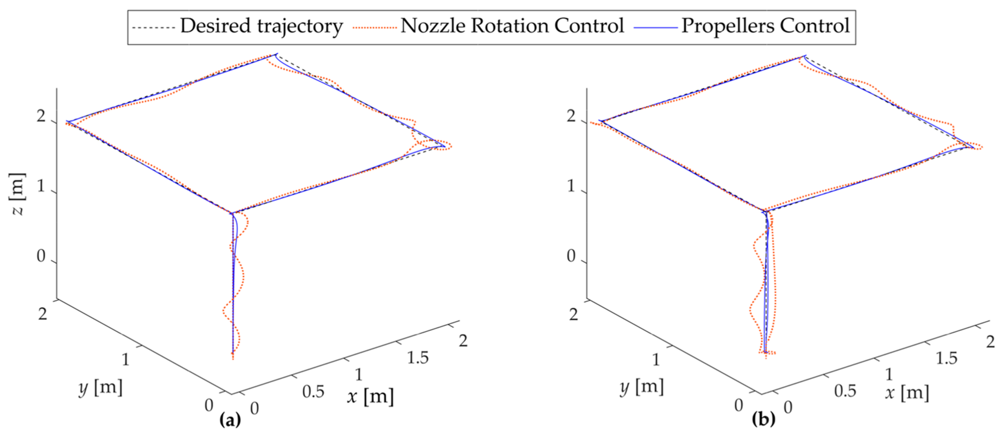
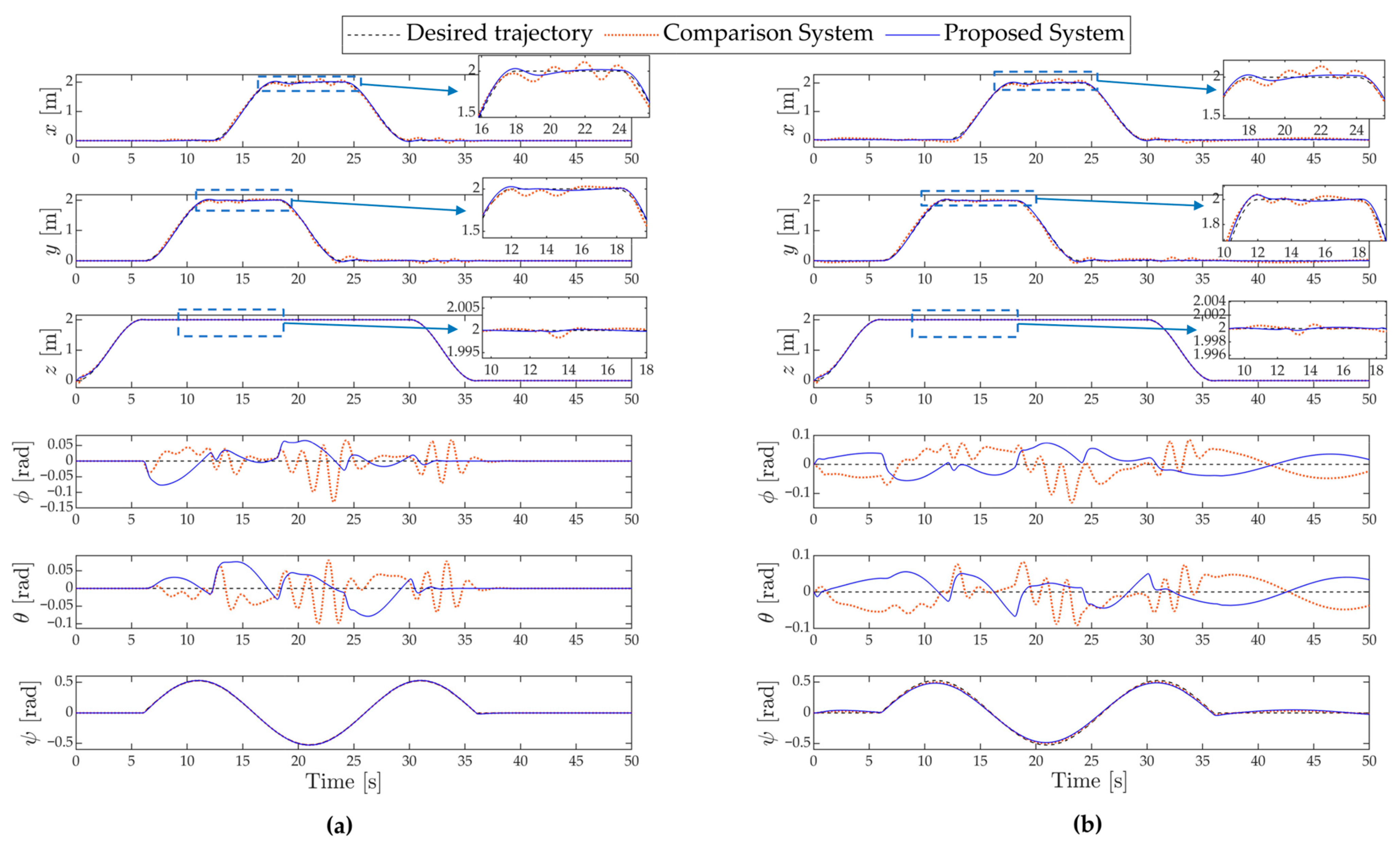
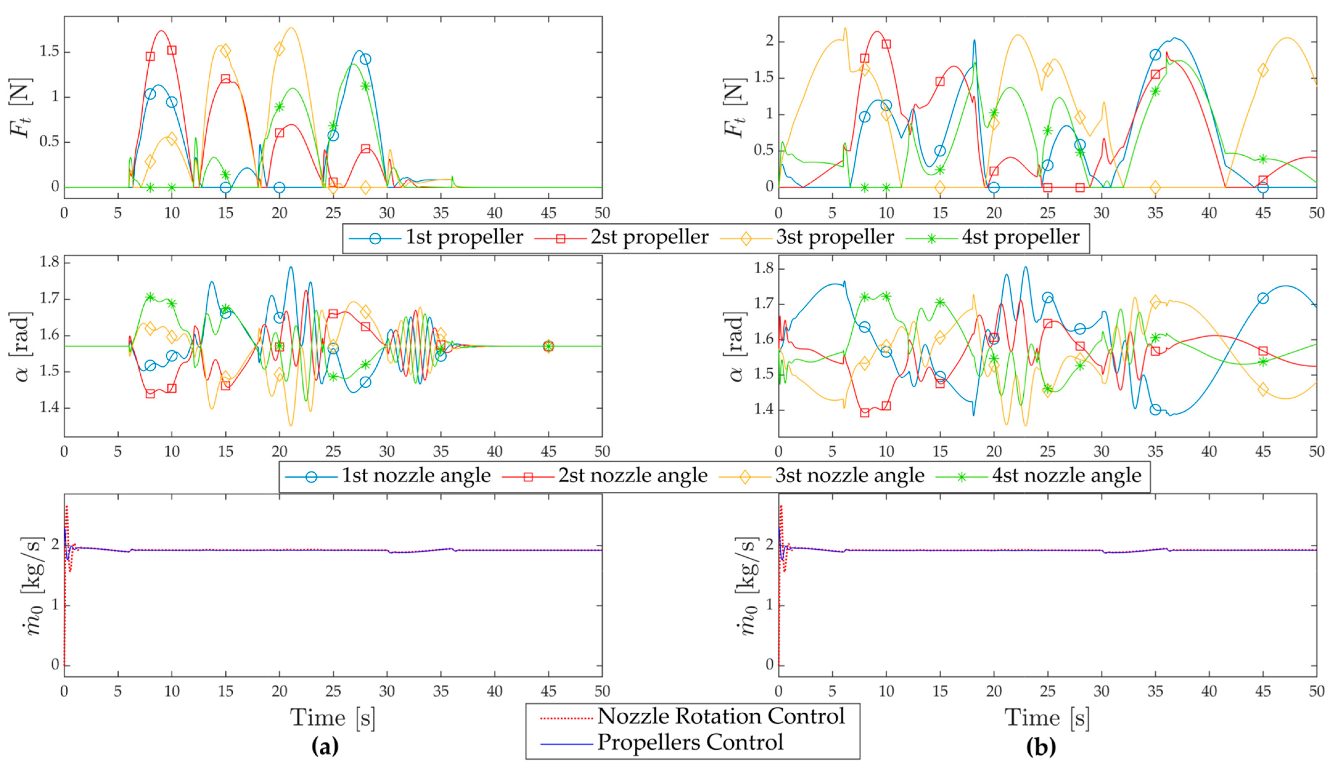
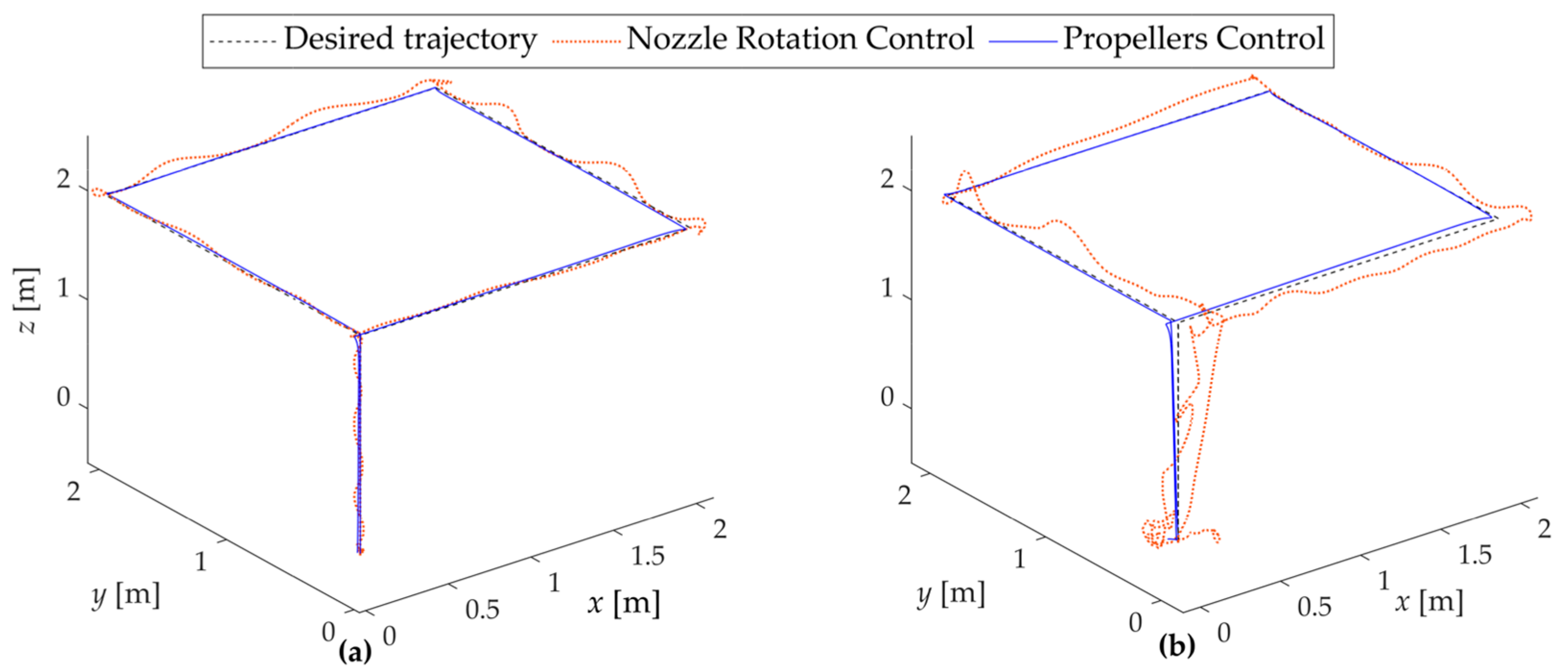
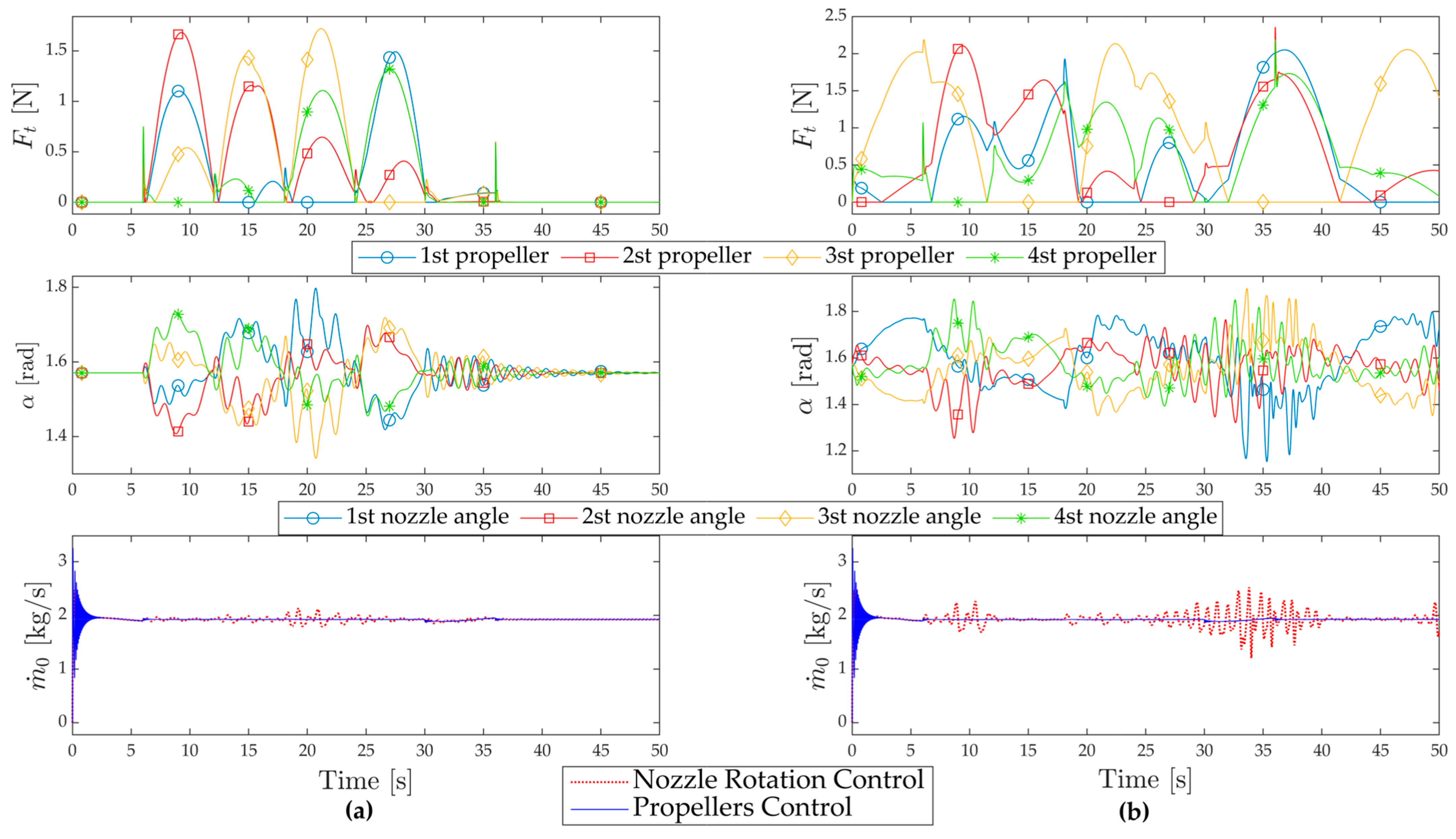
In this study, comparative simulations demonstrate that both flying robots are capable of following the desired reference trajectories effectively. However, the propeller control system exhibits superior performance in terms of tracking accuracy and robustness. Consequently, the propeller control system is selected for further development. In addition, the simulation results contribute to the precise selection of key devices, including the propeller, water distributor, and water pump.

Despite these promising outcomes, a key limitation lies in the system’s reliance on accurate modeling for effective control, particularly under highly dynamic water conditions and water pipe oscillations. For future work, more advanced control techniques will be explored to enable greater flexibility in executing complex trajectories. Furthermore, integrating the propeller control system with the nozzle rotation control system will be considered to further enhance the flying robot’s overall performance. Finally, experimental studies will be conducted to validate the proposed approaches and simulation findings.