Article

Gaussian Process Regression-Based Fixed-Time Trajectory Tracking Control for Uncertain Euler–Lagrange Systems

Key Laboratory of Intelligent Bionic Unmanned Systems, Ministry of Education, School of Intelligence Science and Technology, University of Science and Technology Beijing, Beijing 100083, China
*
Author to whom correspondence should be addressed.
Actuators 2025, 14(7), 349; https://doi.org/10.3390/act14070349
Submission received: 18 June 2025 / Revised: 9 July 2025 / Accepted: 11 July 2025 / Published: 16 July 2025
(This article belongs to the Section Aerospace Actuators)

Abstract

The fixed-time trajectory tracking control problem of the uncertain nonlinear Euler–Lagrange system is studied. To ensure the fast, high-precision trajectory tracking performance of this system, a non-singular terminal sliding-mode controller based on Gaussian process regression is proposed. The control algorithm proposed in this paper is applicable to periodic motion scenarios, such as spacecraft autonomous orbital rendezvous and repetitive motions of robotic manipulators. Gaussian process regression is employed to establish an offline data-driven model, which is utilized for compensating parametric uncertainties and external disturbances. The non-singular terminal sliding-mode control strategy is used to avoid singularity and ensure fast convergence of tracking errors. In addition, under the Lyapunov framework, the fixed-time convergence stability of the closed-loop system is rigorously demonstrated. The effectiveness of the proposed control scheme is verified through simulations on a spacecraft rendezvous mission and periodic joint trajectory tracking for a robotic manipulator.

1. Introduction

Euler–Lagrange systems are a large class of practical control systems, including rigid robotic manipulators, aircraft, spacecraft, and so on. These practical objects have been popularly employed in many related fields, including military affairs and manufacturing. Trajectory tracking of Euler–Lagrange systems has always been a research hotspot. Because of the uncertainties of the dynamic model, the existence of unknown external disturbances, and the coupling effect, it is hard for Euler–Lagrange systems to complete the trajectory tracking control task precisely and quickly, which makes the study on the trajectory tracking control of Euler–Lagrange systems exceedingly challenging.
Fractional sliding-mode control can guarantee system convergence in finite time. Based on the fractional sliding-mode surface, researchers have studied a number of sliding-mode control schemes with the features of converging in finite time [1,2]. In [3], a novel adaptive fuzzy terminal sliding-mode (AFTSM) controller was proposed to control an uncertain system that contains disturbances. The fuzzy logic system was used to approximate the dynamics of a nonlinear control system, which improved the tracking accuracy and robustness of the control system. However, the scheme is suitable for the second-order nonlinear system with the matched disturbance, especially in the circumstance of the lack of mismatch. In [4], a linear sliding surface based on a polynomial reference trajectory was presented, which converged the trajectory tracking error within finite time. Linear state feedback can realize finite-time tracking and allocate convergence time arbitrarily beforehand. However, if the error between the initial measurement and the real state is small, the finite-time convergence cannot be realized.
Based on the finite-time stability of the terminal sliding surface, scholars proposed the fixed-time stability. Fixed-time stability was first discovered in [5] and defined in [6]. It was assumed that the settling time is unrelated to the initial states and is uniformly bounded. In [7], a control approach for fixed-time terminal sliding mode was introduced for a kind of second-order nonlinear systems with matching uncertainty and perturbation. It ensured a predictable time for convergence regardless of the initial states, greatly facilitating practical applications. In [8], a cascade control structure based on a fixed-time stability distributed observer was proposed, which realized fixed-time consistent tracking control. A fixed-time controller was employed in a high-order integrator multi-agent system, which expanded the application scope. In [9], the research progress and the latest research results of fixed-time collaborative control of multi-agent systems were reviewed, and there were some challenging problems in this field.
Intelligent learning methods are certainly developing rapidly today, and as a result, an increasing number of control schemes are employed to approximate the unknown dynamics of control systems to complete high-accuracy tracking control tasks [10,11,12,13]. Gaussian process regression (GPR) is a data-driven supervised learning method that requires a small prior knowledge of arbitrary functions and a good trade-off between generalization and smoothness for small datasets [14,15]. In [16], a data-driven method based on GPR was applied to the feed-forward compensation of system uncertain dynamics, and a high-accuracy trajectory tracking effect was achieved in the circumstance of low feedback gain. However, this study did not extend GPR to other control methods. In [17], GPR and quaternion-based command filtering backstepping control framework were proposed. The control body structure based on GPR used a Bayesian nonparametric representation to estimate the perturbation distribution, which made the control system have good robust performance. In [18], a control framework based on the uncertain control Lyapunov method for Gaussian process modeling was proposed for affine systems. The model fidelity estimation of the Gaussian process model was used to finally achieve high probability asymptotic stability. Both [17,18] employed non-parametric estimation methods to effectively handle noise with minimal prior knowledge. In [19], a trajectory tracking method for underdriven balancing robots based on GP was presented. GP models capture coupling effects between driven and non-driving subsystems through constructed equilibrium manifolds. The algorithm of data selection was adopted to achieve a better tracking effect. However, the GP-based learning method was used for estimating the system’s uncertain dynamics of the robots; the unknown interference was not compensated [20]. In recent work [21], a GP-based adaptive sliding-mode controller was presented, which enabled the tracking error to converge to zero with high probability. Simulation examples illustrated effectiveness and superiority. Based on [21], a GPR-based fixed-time controller is designed.
For Euler–Lagrange systems with uncertainties, a control method combining non-singular terminal sliding-mode control with GPR is designed in this paper. This control system has the feature of fast convergence in fixed time. The stability of the closed-loop control system is proved, and all signals are proved to be bounded. The effectiveness and superiority of the algorithm are proven by simulations. The following are the primary contributions and unique innovations of this article. (1) Compared with previous work [21], this article combines non-singular terminal sliding-mode control with GPR to study the trajectory tracking of a kind of Euler–Lagrange systems. The stability of the system is analyzed under the probability-based Lyapunov framework. The tracking error of the system approaches a small region around zero with high probability. (2) In periodic motion scenarios, the method of data-driven offline learning is used to predict and fit the parametric uncertainties and external disturbances of the control system, which allows the system to realize a better tracking effect under the condition of low gains. The rationality and rigor of the above control method are verified through spacecraft rendezvous missions and robotic manipulator joint trajectory tracking.
The rest of this paper is structured as follows. Section 2 presents GPR and the theory of fixed-time stability. In Section 3, the model of the Euler–Lagrange system is described and the research problem is presented. In Section 4, a GPR-based fixed-time controller is proposed, and the stability of the control system is proved. Section 5 shows the numerical simulations.

2. Preliminaries

Notations: R n × n is a set of n × n real matrices, and R n and R + are a set of n-dimensional real vectors and positive real numbers, respectively. · and | · | denote the Euclidean vector norm and the absolute value, respectively. For a vector z = z 1 , z 2 , , z n and a constant γ , we define sig γ ( z ) = | z 1 | γ sign ( z 1 ) , | z 2 | γ sign ( z 2 ) , , | z n | γ sign ( z n ) , where sign ( · ) is the standard signum function.

2.1. Gaussian Process Regression

The GP is a stochastic real function or discrete function f GP ( x , χ ) that is measurable function of x L and χ Ω , where the set L R n with n N * represents the index set and Ω is the sample space. The GP is entirely assigned by its mean function m ( x ) and covariance function k ( x , x ) as the measurement of the relevance of points x and x . m ( x ) is usually assigned to zero, since there is no previous knowledge available of m ( x ) . In this paper, the GP is described as
f ( x ) GP ( m ( x ) , k ( x , x ) ) , f ( x ) : R n R n , x , x L
to approximate a nonlinear function f ( x ) . The measurement value of f ( x ) is expressed as y = f ( x ) + ω , where ω N ( 0 , diag { σ 1 2 , σ 2 2 , , σ n 2 } ) represents Gaussian noise with the standard deviation σ 1 , σ 2 , , σ n .
The training of the GP needs to be equipped with input and output pairs. Therefore, the training data pairs are defined as D = X , Y with training input matrix X = [ x 1 , x 2 , , x l ] R n × l and training output matrix Y = [ y 1 , y 2 , , y l ] R l × n . The prediction output value of y * R at test value x * R n is a Gaussian distributed variable attained from a Gaussian joint distribution
Y y * N 0 , k ( X , x * ) K ( X , X ) + σ d 2 I N k ( x * , x * ) k ( X , x * )
where σ d is the standard deviation of Gaussian noise; I N is an identity matrix; the matrix function K ( X , X ) R n × n is covariance matrix, where each element denotes the covariance between two points of training input data set X; and the covariance function k ( X , x * ) R l represents the covariance between x * and X. In this paper, the squared exponential covariance function with the set of hyperparameters ϕ = σ n R + * , σ f R + is chosen as the kernel function, which probably is the most generally employed covariance function in GP modeling
k ϕ ( x , x ) = σ f 2 exp x x 2 2 σ e 2
where σ e describes the length-scale, and σ f 2 denotes signal variance, representing the mean distance between f GP ( x ) and m ( x ) . The hyperparameters ϕ = σ f , σ e in the kernel function are trained by the maximum marginal likelihood function [22]
ϕ * = argmax log p ( Y | X , ϕ ) log p ( Y | X , ϕ ) = 1 2 Y ( K + σ n 2 I N ) 1 Y n 2 log ( 2 π ) 1 2 | K + σ d 2 I N |
Remark 1.
For regression methods for nonlinear systems, selecting an appropriate kernel function is more convenient than selecting an appropriate parametric structure, because the unique limitation on kernel functions is that the covariance matrix has to be positive-definite. The squared exponential kernel function has the following characteristics. The members of the corresponding reproducing kernel Hilbert space (RKHS) can consistently and accurately approximate a continuous function on the compact set. A detailed description of the kernels and their respective properties is provided in [23].
The conditional Gaussian distribution of the prediction of f * is obtained with
μ ( f i * | x * , X , Y ) = k ϕ ( x * , X ) ( K ϕ + σ d 2 I N ) 1 Y i var ( f i * | x * , X , Y ) = k ϕ ( x * , x * ) k ϕ ( x * , X ) ( K ϕ + σ d 2 I N ) 1 k ϕ ( x * , X )
GP is generally used for performing multiple regression, so a regression of n outputs needs n GPs. The n-dimensional multi-variable distribution is
f * | x * , D N ( μ ( f * | x * , D ) , ( f * | x * , D ) ) μ ( f * | x * , D ) = [ μ ( f 1 * | x * , D ) , , μ ( f n * | x * , D ) ] ( f * | x * , D ) = diag { var ( f 1 * | x * , D ) , , var ( f n * | x * , D ) }
A part of the prediction variance in x * can be obtained by marginalizing. φ * R n 1 is assumed as a subset of x * with n 1 n . The marginal variance of φ * is
var ( f i * | φ * , X , Y ) = k ϕ ( φ * , φ * ) k ϕ ( φ * , X ) ( K ϕ + σ d 2 I N ) 1 k ϕ ( φ * , X )
At the same time, the hyperparameter set is also reduced to a dimension corresponding to φ * . Therefore, the combined marginal variance can be written as
( f * | φ * , D ) = diag { var ( f 1 * | φ * , D ) , , var ( f n 1 * | φ * , D ) }
Lemma 1
([16]). Consider a nonlinear uncertain system where each component of the function f is approximated by the corresponding GP. As f has a bounded RKHS norm on the known kernel function k, that is, f k , the model error is bounded by
P μ ( f | x * , D ) f ( x * ) ϑ 1 2 ( f | x * , D ) η
where η ( 0 , 1 ) is the probability, ϑ R n , ϑ j = 2 f j k 2 + 300 κ j ln 3 l 1 η 1 n 1 2 , κ R n , κ j = max 1 2 ln | I N + σ j 2 k j ( x , x ) | is the maximum information gain, and I N is an identity matrix.

2.2. Fixed-Time Stability Theory

Consider a system of nonlinear differential equations
x ˙ ( t ) = f ( x ( t ) ) , x ( 0 ) = x 0 , f ( 0 ) = 0
where x = [ x 1 , x 2 , , x n ] ; f ( x ) : K R n is continuous on an open neighborhood K R n of the origin.
Definition 1
([24]). For (8), if the origin and the positive-definite settling time function T ( x ) : D 0 ( 0 , ) have an open neighborhood D K , such that, for all x 0 D 0 , satisfy lim t T ( x 0 ) x ( t ) = 0 for any t [ 0 , T ( x 0 ) ) , then one can conclude that the zero solution of (8) is finite-time convergent. If the origin satisfies both finite-time convergence and Lyapunov stability, the origin is finite-time stable. Moreover, the origin is called as globally finite-time stability when D = K = R n .
However, the settling time of finite-time stability in Definition 1 relies on the system’ initial states, which limits practical application. The theory of fixed-time stability was presented in [6].
Definition 2.
For system (8), the origin is called as fixed-time stability equilibrium if it is globally finite-time stable and the settling time function  T ( x 0 )  is bounded, that is, ∃  T m a x , T ( x 0 ) T m a x , for all x 0 R n .
Lemma 2
([6,25]). Considering (8), one assumes that there is a positive-definite Lyapunov function V ( x ) satisfying
V ˙ ( x ) α V ( x ) a + β V ( x ) b p + ζ
where α, β, a, b, p, and ζ are positive parameters satisfying a p < 1 , b p > 1 and 0 < ζ < . Then, the origin of (8) is fixed-time stable. Furthermore, the state of system converges to the residual set Ω x in fixed-time T, which can be expressed as
Ω x = x | x min α p ζ 1 θ 1 p a , β p ζ 1 θ 1 p b
where θ is a scalar satisfying 0 < θ < 1 . The convergence time is denoted as
T 1 α p θ p ( 1 a p ) + 1 β p θ p ( b p 1 )
Remark 2.
According to Lemma 2, one can know that the upper-bound prior value of the convergence time is independent of the initial states of the system, but only related to the parameters α, β, a, b, p, and θ in (10). This means that the designer can choose the right parameters to ensure the convergence time according to the specific requirements.
Lemma 3
([26]). For z j R , ( j = 1 , 2 , n ) , 0 < r 1 1 and r 2 > 1 , the inequalities below are satisfied.
j = 1 n | z j | r 1 j = 1 n | z j | r 1 j = 1 n | z j | r 2 n r 2 1 j = 1 n | z j | r 2

3. Problem Statement

Consider the dynamic model of the Euler–Lagrange system as
H ( q ) q ¨ + C ( q , q ˙ ) q ˙ + g ( q ) = u d ( t ) + u ( t )
where q represents the generalized coordinate of the Euler–Lagrange system; H ( q ) R n × n is the inertial matrix with symmetric and positive-definite; C ( q , q ˙ ) and g ( q ) are the Coriolis force matrix and the gravitational force vector, respectively; u d ( t ) is the external disturbance vector; u ( t ) is the control input vector. In the actual modeling process, the dynamic model of the Euler–Lagrange system contains unknown modeling dynamics. Define them as follows:
H ( q ) = H 0 ( q ) + H d ( q ) C ( q , q ˙ ) = C 0 ( q , q ˙ ) + C d ( q , q ˙ ) g ( q ) = g 0 ( q ) + g d ( q )
where H 0 ( q ) , C 0 ( q , q ˙ ) , and g 0 ( q ) are known dynamics, and H d ( q ) , C d ( q , q ˙ ) , and g d ( q ) are unknown dynamics of H ( q ) , C ( q , q ˙ ) , and g ( q ) , respectively. Combining (12), the dynamics (11) is rewritten as
q ¨ = H 0 1 ( q ) u ( t ) + d ( t )
where d ( t ) = H 1 ( q ) u d ( t ) + H 1 ( q ) C ( q , q ˙ ) q ˙ g ( q ) + H ˜ d ( q ) u ( t ) is a compound disturbance of a Euler–Lagrange system that contains parametric uncertainties and external disturbances. H ˜ d ( q ) = H 1 ( q ) H 0 1 ( q ) .
Assumption 1.
The external disturbance vector u d ( t ) is unknown but bounded by u d ( t ) D ¯ , where D ¯ is a known parameter.
Assumption 2.
The desired state trajectory is second-order continuous differentiable and bounded by q d q ¯ d , q ˙ d q ˙ ¯ d with q ¯ d , q ˙ ¯ d > 0 .
The control objective of this article is to design a fixed-time terminal sliding-mode controller based on GPR, which satisfies Assumptions 1 and 2 so that the trajectories q and q ˙ of the system can track the desired trajectories q d and q ˙ d .

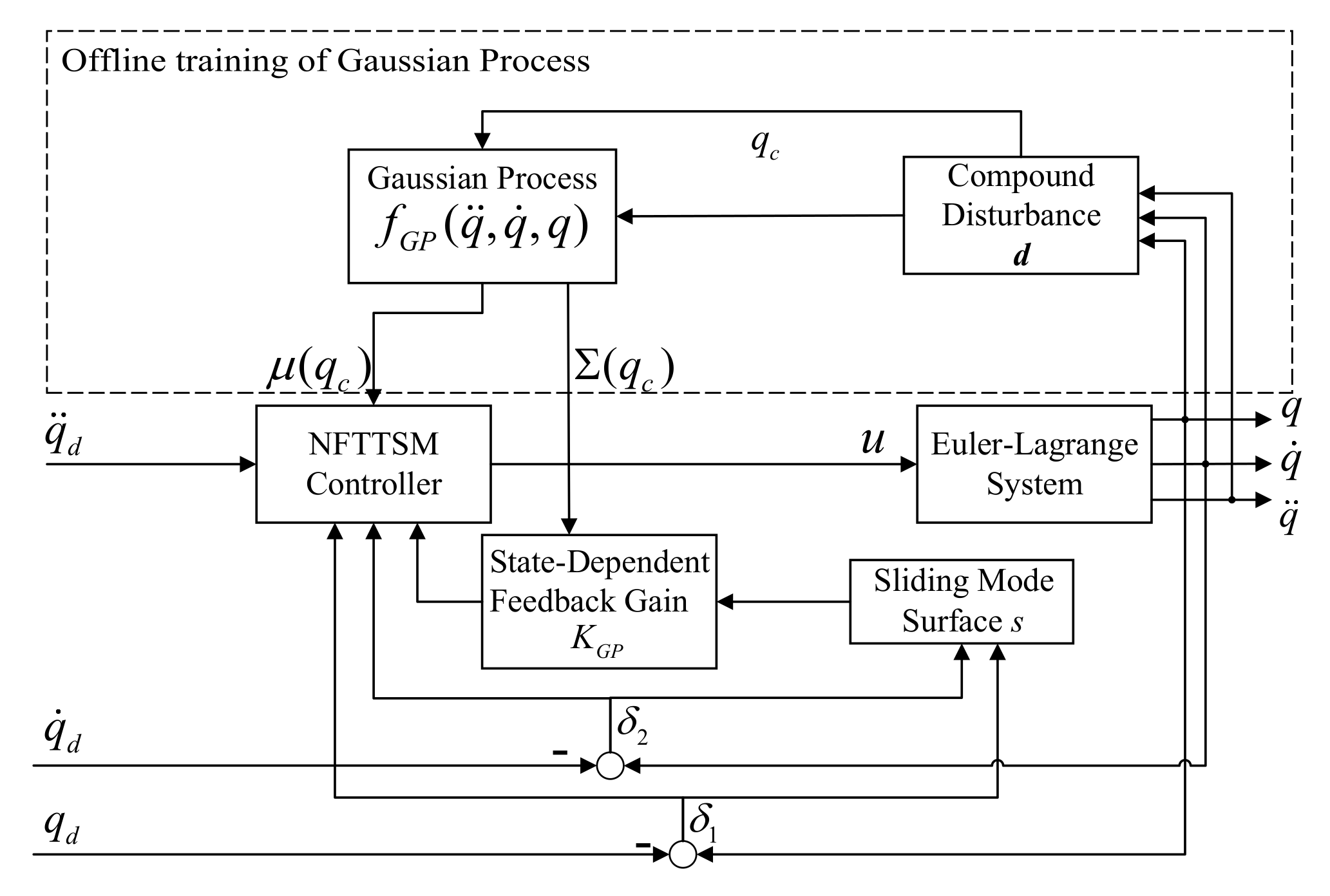
4. Controller Design and Stability Analysis

The tracking errors can be defined as
δ 1 = q q d δ 2 = q ˙ q ˙ d
where q d and q ˙ d denote the desired trajectory and its derivative, respectively.
Based on (13) and (14), the error dynamics of a Euler–Lagrange system can be denoted as
δ 1 ˙ = δ 2 δ 2 ˙ = H 0 1 u + d q ¨ d
In this section, a GP-based non-singular fixed-time terminal sliding-mode (GP-NFTTSM) controller is presented to achieve the control objective. The major reason for selecting NFTTSM is that it has the benefits of fast convergence and avoidance of singularity. GPs are utilized to compensate for the modeling uncertainties as well as external interferences, which enhances the anti-interference ability of the system and boosts the control performance.
For system (11), a novel NFTTSM surface is introduced as follows [27]:
s = R ( δ 1 ) δ 1 + sig ρ 2 ( δ 2 )
where R ( δ 1 ) = diag r ( δ 11 ) , r ( δ 12 ) , , r ( δ 1 n ) is a diagonal matrix and r ( δ 1 j ) , ( j = 1 , 2 , , n ) is expressed as
r ( δ 1 j ) = α | δ 1 j | p 1 r ρ 2 + β | δ 1 j | e 1 r ρ 2 r ρ 2
where α > 0 , β > 0 , r > 1 and ρ 2 > 1 , and p and e are positive parameters satisfying e r > 1 and 1 ρ 2 < p r < 1 .
Based on (16) and Notations in Preliminaries, the sliding-mode dynamics are expressed as
s ˙ = d R ( δ 1 ) d t δ 1 + R ( δ 1 ) δ 2 + ρ 2 Δ 2 δ ˙ 2 = R ¯ ( δ 1 ) δ 2 + R ( δ 1 ) δ 2 + ρ 2 Δ 2 δ ˙ 2
where Δ 2 = diag | δ 21 | ρ 2 1 , | δ 22 | ρ 2 1 , , | δ 2 n | ρ 2 1 , R ¯ ( δ 1 ) = diag r ¯ ( δ 11 ) , r ¯ ( δ 11 ) , , r ¯ ( δ 1 n ) is a diagonal matrix, and r ¯ ( δ 1 j ) , ( j = 1 , 2 , , n ) is expressed as
r ¯ ( δ 1 j ) = r ρ 2 α | δ 1 j | p 1 r ρ 2 + β | δ 1 j | e 1 r ρ 2 r ρ 2 1 α p 1 r ρ 2 | δ 1 j | p 1 r ρ 2 + β e 1 r ρ 2 | δ 1 j | e 1 r ρ 2
Theorem 1.
Consider the defined sliding-mode variable s in (16). If s = 0 is satisfied, δ 1 and δ 2 will converge to zero in fixed time.
Proof. 
If s = R ( δ 1 ) δ 1 + sig ρ 2 ( δ 2 ) = 0 is achieved, then one has [27]
δ ˙ 1 = sig r [ α sig p ( δ 1 ) + β sig e ( δ 1 ) ]
To prove the convergent nature of variable δ 1 , we define a Lyapunov function v = 1 2 δ 1 δ 1 . Combined with Lemma 3, the time derivative of v is
v ˙ = δ 1 δ ˙ 1 = δ 1 sig r [ α sig p ( δ 1 ) + β sig e ( δ 1 ) ] = i = 1 n δ 1 i sig r [ α sig p ( δ 1 i ) + β sig e ( δ 1 i ) ] = i = 1 n δ 1 i | α sig p ( δ 1 i ) + β sig e ( δ 1 i ) | r sign [ α sig p ( δ 1 i ) + β sig e ( δ 1 i ) ] = i = 1 n δ 1 i | α | δ 1 i | p sign ( δ 1 i ) + β | δ 1 i | e sign ( δ 1 i ) | r sign [ α | δ 1 i | p sign ( δ 1 i ) + β | δ 1 i | e sign ( δ 1 i ) ] = i = 1 n δ 1 i α | δ 1 i | p + β | δ 1 i | e r sign ( δ 1 i ) = i = 1 n | δ 1 i | α | δ 1 i | p + β | δ 1 i | e r = i = 1 n α ( | δ 1 i | 2 ) 1 + p r 2 r + β ( | δ 1 i | 2 ) 1 + e r 2 r r n 1 r α i = 1 n ( | δ 1 i | 2 ) 1 + p r 2 r + β i = 1 n ( | δ 1 i | 2 ) 1 + e r 2 r r n 1 r ω 1 v 1 + p r 2 r + ω 2 v 1 + e r 2 r r
where ω 1 = 2 1 + p r 2 r α and ω 2 = 2 1 + e r 2 r β . Thus, from [6], it can be concluded that δ 1 converges to zero in fixed-time T 2 , which is irrelevant to the initial states. Moreover, based on the error dynamics (15), we obtain s = 0 and lim t T 2 δ 1 ( t ) = 0 . Similarly, it can also be concluded that δ 2 converges to zero in fixed time. According to Lemma 2, we obtain
T 2 2 n 1 r ω 1 r θ r ( 1 p r ) + 2 n 1 r ω 2 r θ r ( e r 1 )
Next, the application of the GP in the controller design is stated.
In this paper, the GP learns the truth of function d ( t ) in (13) which contains the modeling uncertainties and the external disturbances. The dataset of the GP is denoted as D = q c , i , d i , ( i = 1 , 2 , , m ) which contains m data pairs, where q c = q ¨ , q ˙ , q R 3 n is the input data and d is the output data. Algorithm 1 illustrates the process of generating a dataset for GP training.
Algorithm 1 Data Generation for GP Learning.
 1:
Define a desired trajectory q d ( t ) for the system, then we can obtain q ˙ d ( t ) and q ¨ d ( t ) . The initial velocity q ˙ 0 and initial acceleration q ¨ 0 are set to zero.
 2:
m data pairs are generated uniformly in the state space as initial state q 0 and control torque.
 3:
The control torque in step 2 is exerted to system, then the position q , velocity q ˙ and acceleration q ¨ are recorded.
 4:
Based on (13) and step 3, we can obtain q ¨ , q ˙ , q and d .
 5:
The last step is collecting the dataset, that is, X q ¨ , q ˙ , q and Y d .
Remark 3.
Since GPR performance is highly dependent on data quality and selection, for uniformly generated initial states and control torques, theoretically, q , q ˙ and q ¨ recorded should not exhibit significant abrupt changes. However, due to the interference of system noise, the actual state of the data is uncertain. To address this, we manually select the data by retaining relatively smooth ones and eliminating those with large fluctuations, thereby improving the quality of the dataset.
After recording the training data pairs, the hyperparameters in the kernel function are trained using the maximum marginal likelihood function (3). Then, we construct a GP model f G P which has n Gaussian process posterior kernels with exponential squared functions
f G P ( q c ) = f G P 1 N ( μ 1 ( q c ) , var 1 ( q c ) ) f G P 2 N ( μ 2 ( q c ) , var 2 ( q c ) ) f G P n N ( μ n ( q c ) , var n ( q c ) ) ,
where
μ ( q c ) = k ϕ 1 ( x * , X ) ( K ϕ 1 + σ d 2 I N ) 1 Y 1 k ϕ 2 ( x * , X ) ( K ϕ 2 + σ d 2 I N ) 1 Y 2 k ϕ n ( x * , X ) ( K ϕ n + σ d 2 I N ) 1 Y n .
μ ( q c ) is used to approximate the truth value of d to compensate for the modeling uncertainties and the external disturbances.
Assumption 3.
Let the function p = diag { var ( d | q 1 , q ˙ 1 , D ) , , var ( d | q n , q ˙ n , D ) } : R n R n × n be the marginal variance that is defined by (6). K G P ( p ) : R n × n R n × n is a positive-definite diagonal matrix called variable feedback gain, which is denoted as K G P ( p ) = diag K G P , 11 ( 1 ) , , K G P , p p ( p ) + K c with K c R n × n . In addition, each diagonal element of K G P ( p ) is continuous and bounded by
k p 1 x 2 x K G P ( p ) x k p 2 x 2
for any q , q ˙ , x R n with k p 1 , k p 2 R + .
Remark 4.
During the selection of the training dataset, the area of the training point should resemble the desired operating area, and the dataset can be trained using the method of maximum likelihood optimization. When the quantity of training points approaches infinity, the tracking error is largely asymptotically convergent. The main advantage of using state-dependent feedback gain is that the confidence of the model is incorporated into the feedback control, and the feedback gain can be adjusted according to the confidence of the model and achieve robust performance. The choice of state-dependent feedback gain is enlightened from [28].
Then, we proceed to the design of the equivalent control law u e q ( t ) . If the system dynamics are known, u e q ( t ) keeps the states of the system on the sliding surface and eventually converges. However, in practical applications, system dynamics cannot be fully known. To allow the states of the system to meet the sliding requirement under the circumstances of external interferences and modeling uncertainties, we design the following control law u s w ( t ) .
u e q ( t ) = H 0 ( q ) 1 ρ 2 ( R ¯ ( δ 1 ) + R ( δ 1 ) ) sig 2 ρ 2 ( δ 2 ) q ¨ d + μ ( q c )
u s w ( t ) = H 0 ( q ) 1 ρ 2 Δ 2 1 sig ρ 4 ( ρ 5 sig ρ 1 ( s ) + ρ 6 sig ρ 3 ( s ) ) + K G P ( p ) s
where ρ 4 > 1 , ρ 4 ρ 1 < 1 , 1 < ρ 3 ρ 4 < ρ 4 , ρ 5 , and ρ 6 are positive constants. The GP-NFTTSM controller can be designed as
u ( t ) = u e q ( t ) + u s w ( t )
The structure of the proposed closed-loop controller is shown in Figure 1. The offline learning system of the GP regression model deals with compound disturbance in similar motion scenarios, encompassing the modeling uncertainties and external disturbances. The mean μ ( q c ) and variance ( q c ) of the GP are employed to compensate for the system compound disturbance and control gains, respectively. q is the vector of actual position, q d is the vector of desired position, and u is the vector of control input.
Theorem 2.
Consider the trajectory tracking and Euler–Lagrange dynamics system (11) with Assumptions 1 and 2. The control law (25) guarantees that the sliding-mode variable s converges to a small neighborhood of zero Ω s in fixed-time T 1 with a probability of at least η. Therefore, the tracking errors δ 1 and δ 2 of the system also converge to a small neighborhood of zero in fixed time with a probability of at least η. The upper bound of the convergence time is given by the following inequality
T < T m a x = T 1 + T 2
where
T 1 = 2 n 1 ρ 4 ( 2 ( 1 + ρ 1 ρ 4 ) / ( 2 ρ 4 ) ρ 5 θ ) ρ 4 ( 1 ρ 1 ρ 4 ) + 2 n 1 ρ 4 ( 2 ( 1 + ρ 3 ρ 4 ) / ( 2 ρ 4 ) ρ 6 θ ) ρ 4 ( ρ 3 ρ 4 1 )
T 2 = 2 n 1 r 2 ( 1 + p r ) / 2 ψ α r θ ( 1 p r ) + 2 n 1 r 2 ( 1 + e r ) / 2 ψ β r θ ( e r 1 )
Proof. 
Based on the dynamics of tracking errors (15) and the dynamics of sliding mode (18), one has
s ˙ = R ¯ ( δ 1 ) δ 2 + R ( δ 1 ) δ 2 + ρ 2 Δ 2 H 0 1 u + d q ¨ d
Considering the control law in (25), the dynamics of the closed-loop system is
s ˙ = R ¯ ( δ 1 ) δ 2 + R ( δ 1 ) δ 2 + ρ 2 Δ 2 H 0 1 ( u e q + u s w ) + d q ¨ d = R ¯ ( δ 1 ) δ 2 + R ( δ 1 ) δ 2 + ρ 2 Δ 2 H 0 1 H 0 1 ρ 2 ( R ¯ ( δ 1 ) + R ( δ 1 ) ) sig 2 ρ 2 ( δ 2 ) q ¨ d + μ ( q c ) H 0 1 ρ 2 Δ 2 1 sig ρ 4 ( ρ 5 sig ρ 1 ( s ) + ρ 6 sig ρ 3 ( s ) ) + K G P ( p ) s + d q ¨ d = R ¯ ( δ 1 ) δ 2 + R ( δ 1 ) δ 2 + ρ 2 Δ 2 1 ρ 2 ( R ¯ ( δ 1 ) + R ( δ 1 ) ) sig 2 ρ 2 ( δ 2 ) + q ¨ d μ ( q c ) 1 ρ 2 Δ 2 1 sig ρ 4 ( ρ 5 sig ρ 1 ( s ) + ρ 6 sig ρ 3 ( s ) ) + K G P ( p ) s + d q ¨ d = sig ρ 4 [ ρ 5 sig ρ 1 ( s ) + ρ 6 sig ρ 3 ( s ) ] K G P ( p ) s + ρ 2 Δ 2 d μ ( d | q r , D )
A Lyapunov candidate function V ( t ) = 1 2 s s is chosen to analyze system stability. Then, the time derivative of V ( t ) is
V ˙ ( t ) = s s ˙ = s sig ρ 4 [ ρ 5 sig ρ 1 ( s ) + ρ 6 sig ρ 3 ( s ) ] s K G P s + ρ 2 s Δ 2 d μ ( d | q r , D )
According to the Lemma 1, we know μ ( d | q r , D ) d ϑ 1 2 ( d | q r , D ) with probability η . Substituting the above-mentioned inequality into (31), we obtain
P V ˙ ( t ) s sig ρ 4 [ ρ 5 sig ρ 1 ( s ) + ρ 6 sig ρ 3 ( s ) ] s K G P s + ρ 2 s Δ 2 ϑ 1 2 ( d | q r , D ) η
For the next step, we consider the inequality given by v 1 x v 1 2 / v 2 + v 2 x 2 / 4 that hold x R n and v 1 , v 2 R + , one has ρ 2 s Δ 2 ϑ 1 2 ( d | q r , D ) ρ 2 2 Δ 2 2 ϑ 1 2 ( d | q r , D ) 2 / v 2 + v 2 / 4 s 2 . Moreover, based on Assumption 2, one has s K G P s k p 1 s 2 . Selecting the proper parameter v 2 ensures 0 < v 2 / 4 k p 1 . Therefore, (32) can be expressed as
P V ˙ ( t ) s sig ρ 4 ρ 5 sig ρ 1 ( s ) + ρ 6 sig ρ 3 ( s ) k p 1 s 2 + ρ 2 2 Δ 2 2 ϑ 1 2 ( d | q r , D ) 2 / v 2 + v 2 / 4 s 2 s sig ρ 4 ρ 5 sig ρ 1 ( s ) + ρ 6 sig ρ 3 ( s ) + ρ 2 2 Δ 2 2 ϑ 1 2 ( d | q r , D ) 2 / v 2 i = 1 n ρ 5 ( | s i | 2 ) ( 1 + ρ 1 ρ 4 ) / ( 2 ρ 4 ) + ρ 6 ( | s i | 2 ) ( 1 + ρ 3 ρ 4 ) / ( 2 ρ 4 ) ρ 4 + ρ 2 2 Δ 2 2 ϑ 1 2 ( d | q r , D ) 2 / v 2 n 1 ρ 4 ρ 5 i = 1 n ( | s i | 2 ) ( 1 + ρ 1 ρ 4 ) / ( 2 ρ 4 ) + ρ 6 i = 1 n ( | s i | 2 ) ( 1 + ρ 3 ρ 4 ) / ( 2 ρ 4 ) ρ 4 + ρ 2 2 Δ 2 2 ϑ 1 2 ( d | q r , D ) 2 / v 2 n 1 ρ 4 τ 1 V ( 1 + ρ 1 ρ 4 ) / ( 2 ρ 4 ) + τ 2 V ( 1 + ρ 3 ρ 4 ) / ( 2 ρ 4 ) ρ 4 + Ω 1 η
where τ 1 = 2 ( 1 + ρ 1 ρ 4 ) / ( 2 ρ 4 ) ρ 5 , τ 2 = 2 ( 1 + ρ 3 ρ 4 ) / ( 2 ρ 4 ) ρ 6 , Ω 1 = ρ 2 2 Δ 2 2 ϑ 1 2 ( d | q r , D ) 2 / v 2 . Based on Lemma 2, we can conclude that s will converge to the small neighborhood of zero defined by Ω s in fixed-time T 1 , where
Ω s = min 1 n 1 ρ 4 τ 1 ρ 4 Ω 1 1 θ 2 1 + ρ 1 ρ 4 , 1 n 1 ρ 4 τ 2 ρ 4 Ω 1 1 θ 2 1 + ρ 3 ρ 4
Remark 5.
From Theorem 1, we can deduce that when s tends to the neighborhood of zero, δ 1 and δ 2 also tend to the neighborhood of zero. Therefore, Theorem 1 is mainly used to show that the convergence of δ 1 and δ 2 depends on the convergence of the sliding-mode variable. Theorem 1 states that s = 0 is an attractor in the state space. Thus, as long as the sliding-mode variable s tends to the neighborhood of zero, δ 1 and δ 2 will tend to the neighborhood of zero.
Then, we introduce the proof of the convergences of δ 1 and δ 2 . Once the sliding-mode variable converges to set Ω s , one has
s ¯ = R ( δ 1 ) δ 1 + sig ρ 2 ( δ 2 ) , s ¯ Ω s
then
δ ˙ 1 = sig r α sig p ( δ 1 ) + β sig e ( δ 1 ) + s ¯ 1 r
Select the identical Lyapunov function as Theorem 1 v ( t ) = 1 2 δ 1 δ 1 . According to Theorem 1, one has
P { v ˙ ( t ) = δ 1 δ ˙ 1 n 1 r α i = 1 n ( | δ 1 i | 2 ) 1 + p r 2 r + β i = 1 n ( | δ 1 i | 2 ) 1 + e r 2 r r + δ 1 s ¯ 1 r n 1 r α r i = 1 n | δ 1 i | 1 + p r + β r i = 1 n | δ 1 i | 1 + e r + δ 1 s ¯ 1 r = n 1 r α r i = 1 n | δ 1 i | 1 + p r + ψ β r i = 1 n | δ 1 i | 1 + e r ( 1 ψ ) n 1 r β r i = 1 n | δ 1 i | 1 + e r + δ 1 s ¯ 1 r η
where 0 < ψ < 1 . If | δ 1 i | > s ¯ 1 r n 1 r β r ( 1 ψ ) 1 / e r , one has
P v ˙ ( t ) n 1 r 2 ( 1 + p r ) / 2 α r v ( 1 + p r ) / 2 + 2 ( 1 + e r ) / 2 ψ β r v ( 1 + e r ) / 2 η
Similarly, if | δ 1 i | > s ¯ 1 r n 1 r α r ( 1 ψ ) 1 / p r , one has
P v ˙ ( t ) n 1 r 2 ( 1 + p r ) / 2 ψ α r v ( 1 + p r ) / 2 + 2 ( 1 + e r ) / 2 β r v ( 1 + e r ) / 2 η
Thus, from Theorem 1 and [6], one can conclude that δ 1 i converges to the set Ω δ 1 i in fixed-time T 2 , where
Ω δ 1 i = min s ¯ 1 r n 1 r α r ( 1 ψ ) 1 / p r , s ¯ 1 r n 1 r β r ( 1 ψ ) 1 / e r
Based on (15), s = s ¯ and lim t T 2 δ 1 i ( t ) = Ω δ 1 i , one can also conclude that δ 2 converges to a small neighborhood of zero.
Moreover, the conclusion can be drawn that the closed-loop system is ultimately uniformly locally bounded and convergent to a small neighborhood of zero in fixed-time T = T 1 + T 2 with a probability of at least η . □
Remark 6.
Since the GP-NFTTSM controller is designed using a probabilistic GP model, the stability of the closed-loop system is described in terms of probability in Theorem 2. However, in fact, both the system (11) and the control algorithm (25) are deterministic, so stability analysis of the closed-loop system also relies on the deterministic Lyapunov theory. As long as the control gain is appropriate, the probability in Theorem 2 can be any value in ( 0 , 1 ) , so the existence of probability has no effect on the stability of the control system.

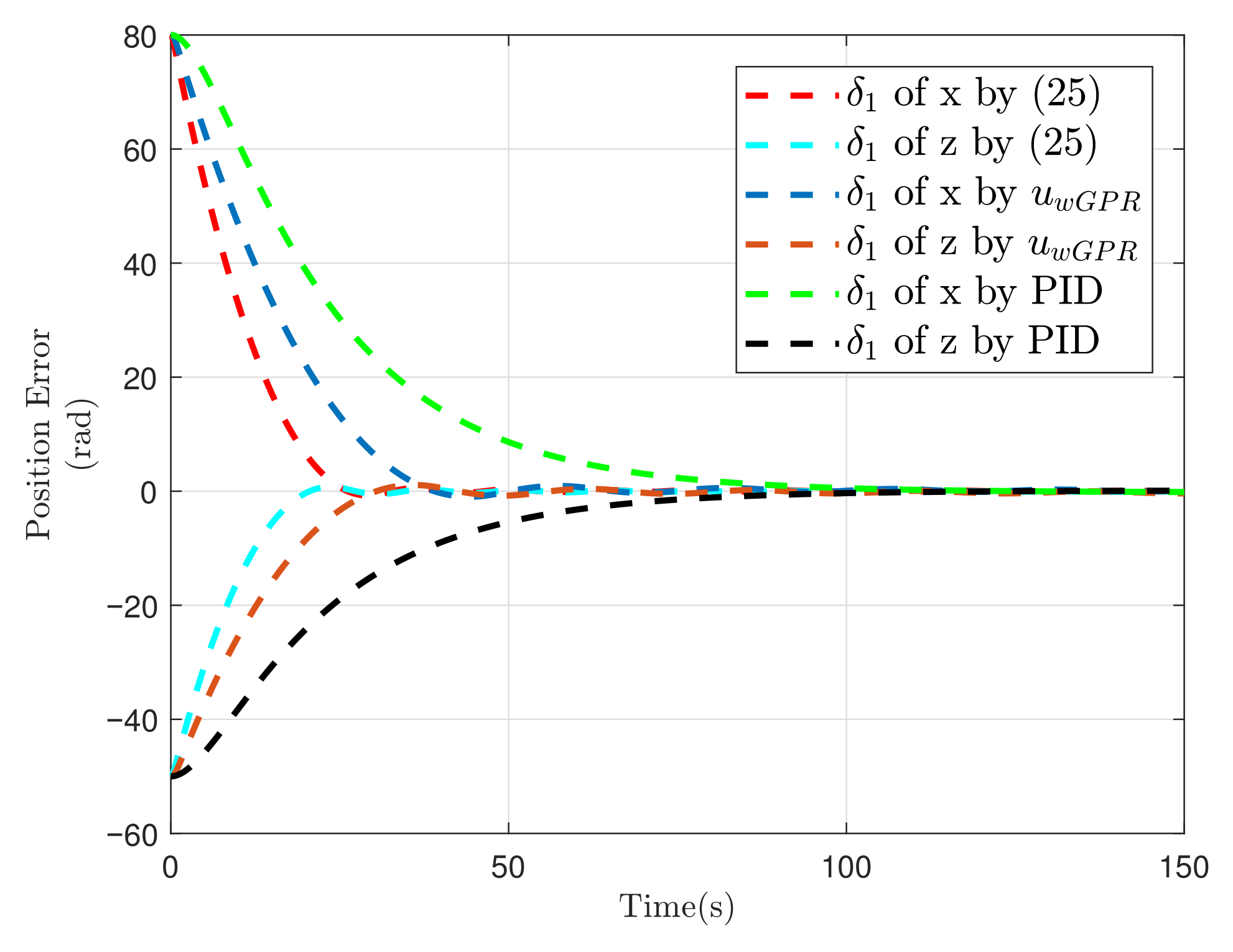
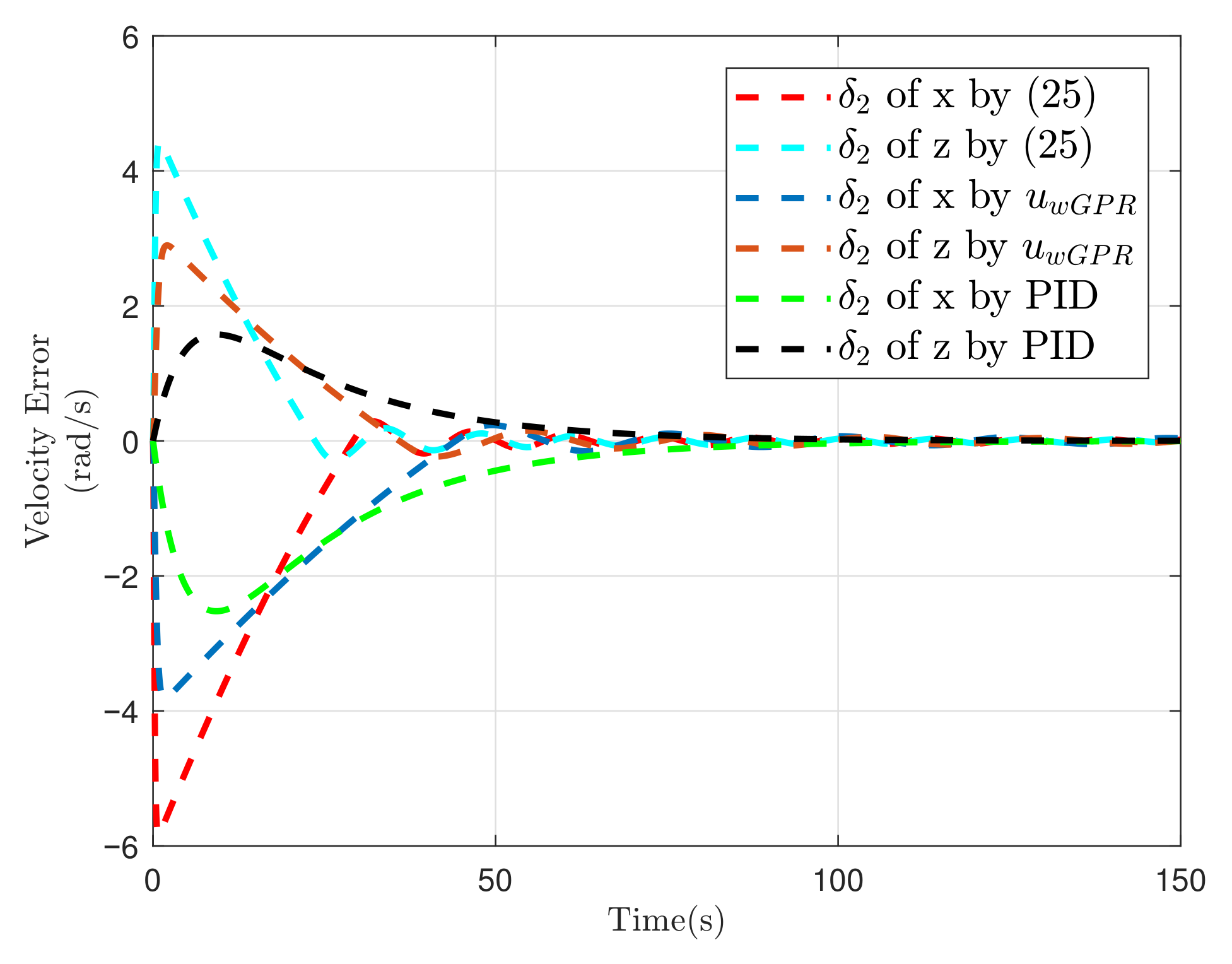
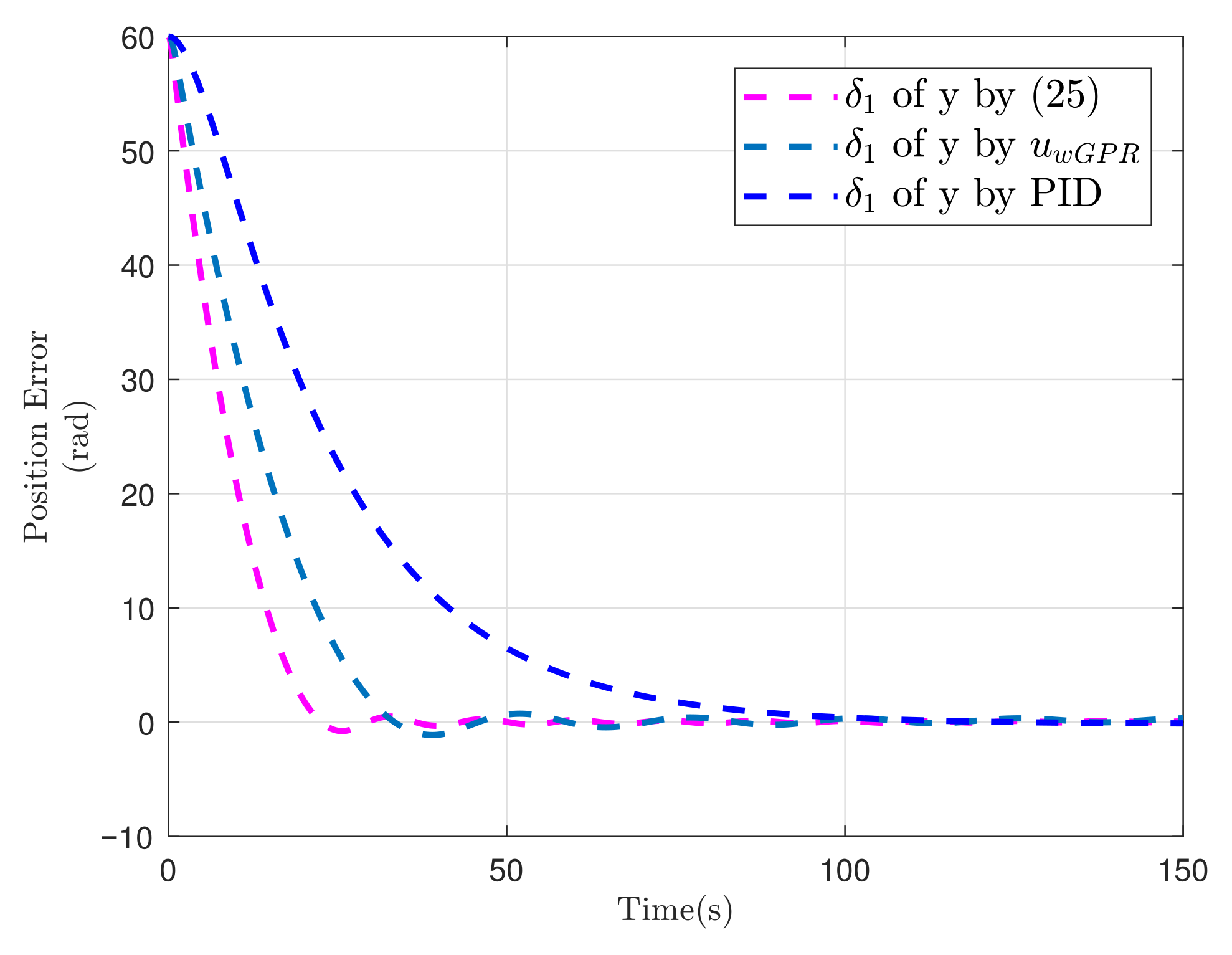
5. Numerical Simulation and Comparisons

For the purpose of verifying the effectiveness of the above-mentioned controller, we adopt the spacecraft rendezvous issue and the trajectory tracking issue of a two-link robotic manipulator for numerical simulations.

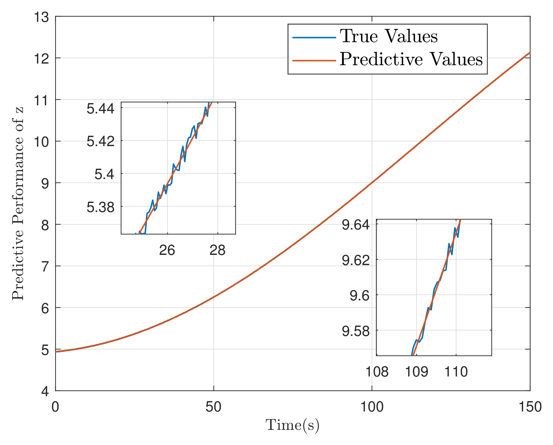
5.1. Simulation of Spacecraft Rendezvous Mission

The spacecraft rendezvous mission involves the execution of a series of orbital maneuvers during the close-proximity phase to nullify the relative positions and velocities between the chaser and the target [29,30,31]. Considering the issue of spacecraft rendezvous, we define e = x , y , z as the relative position of the chaser in the target local orbital coordinate frame. In the case where the orbital angular velocity of the target is precisely known, the dynamic equation is expressed as [32]
H = m c h I 3 , C = m c h C ¯ , g = m c h g ¯ ,
C ¯ = 0 2 n 0 0 2 n 0 0 0 0 0 0 , g ¯ = 3 n 0 2 0 0 0 0 0 0 0 n 0 2 e .
The mass of the chaser is defined as m c h = 300 ( kg ) . The angular velocity of the target orbit is defined as n 0 = 7.2722 × 10 5 ( rad / s ) . In addition, the external disturbance is
u d ( t ) = 2 × 5 + 3.5 sin ( π 100 t ) 1.5 cos ( π 100 t ) 4 2.5 sin ( π 100 t ) + cos ( π 100 t ) 5 + 2.5 sin ( π 100 t ) 0.5 cos ( π 100 t ) .
Then, the desired states are e d = 0 , 0 , 0 and e ˙ d = 0 , 0 , 0 . Assume the initial relative position and relative velocity between two spacecrafts are e ( 0 ) = 80 , 60 , 50 and e ˙ ( 0 ) = 0 , 0 , 0 , respectively. The parameters of NFTTSM controller are α = β = 1 , p = 0.7 , e = 10 / 9 , r = 6 / 5 , ρ 1 = 1 / 3 , ρ 2 = 6 / 5 , ρ 3 = 3 / 4 , ρ 4 = 2 , ρ 5 = ρ 6 = 2 and ϵ = 0.01 . To illustrate the validity of controller (25), the method is compared with the PID controller and the control law u w G P R , which is defined as the controller (25) without GPR. The three parameters of the PID controller are K p = 100 , K i = 0.01 and K d = 250 .
Figure 2, Figure 3, Figure 4 and Figure 5 show the curve of the relative position e and relative velocity e ˙ in three directions. Obviously, e and e ˙ can still converge to the zero neighborhood with external interferences and unmodeled dynamics. Figure 6 illustrates the variation curve of the thrust u of the chaser. Compared with u w G P R , the designed GP-NFTTSM control law has better anti-interference ability. Compared with the PID controller, the designed GP-NFTTSM control law accomplishes faster convergence speed and higher tracking accuracy. Despite its simple form, the PID control law exhibits poor disturbance rejection performance in the presence of significant external disturbances and poses certain difficulties in parameter adjustment. From Figure 7, Figure 8 and Figure 9, one can conclude that GPR can better predict the value of function d ( t ) in (13), which is utilized for compensating external disturbances and parametric uncertainties to enhance the tracking accuracy of Euler–Lagrange systems. The integrated absolute error criterion (IAE, defined by 0 t | δ ( x ) | d x ) and the integrated time absolute error criterion (ITAE, defined by 0 t x | δ ( x ) | d x ) are used to compare the performances of those methods. T p and T v represent the convergence time of position and velocity errors, respectively. e represents the norm steady-state value of error vector. The consequences are shown in Table 1. Obviously, the tracking performances of x, y, and z of controller (25) outperform controller u w G P R and PID.

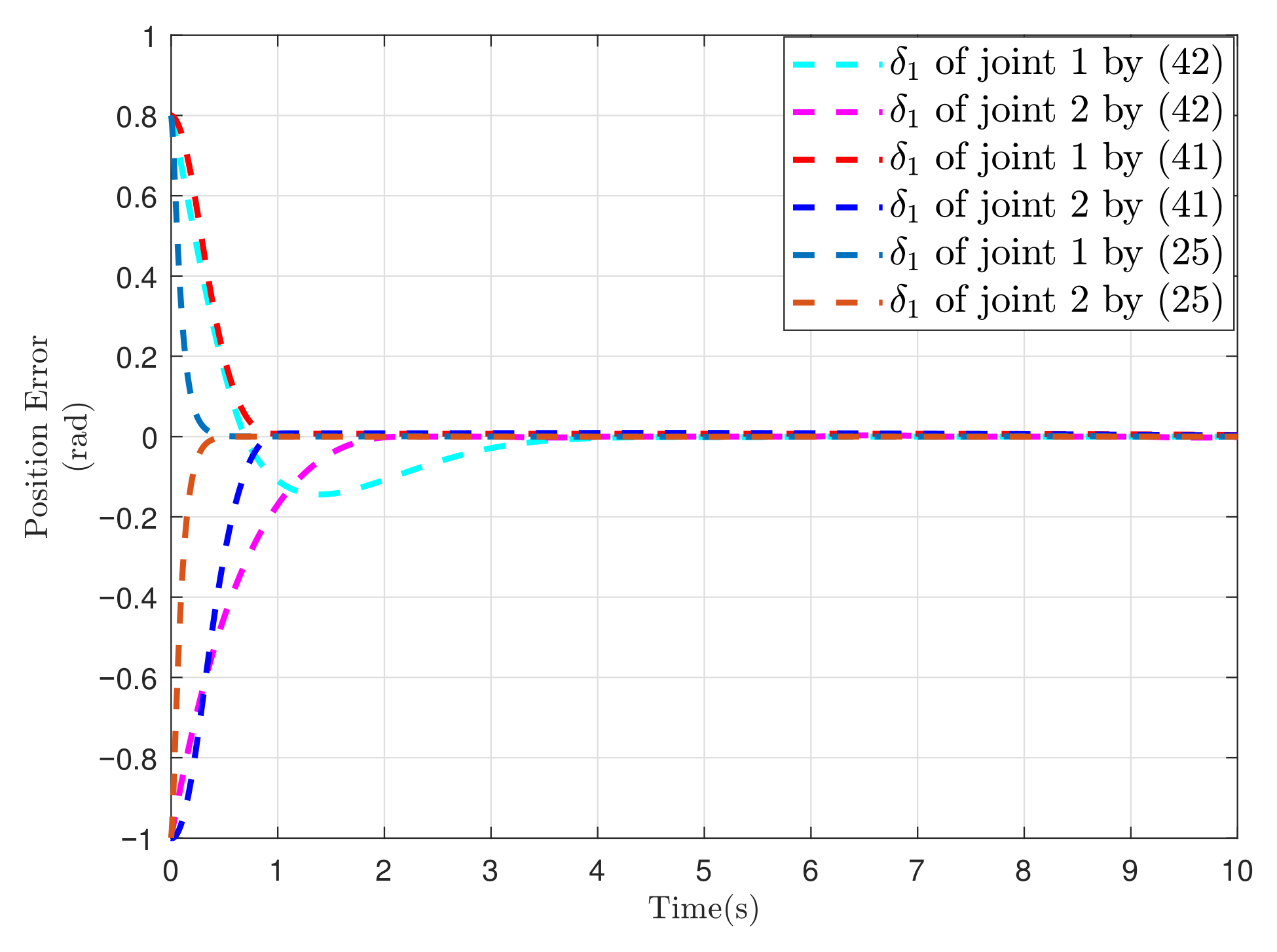
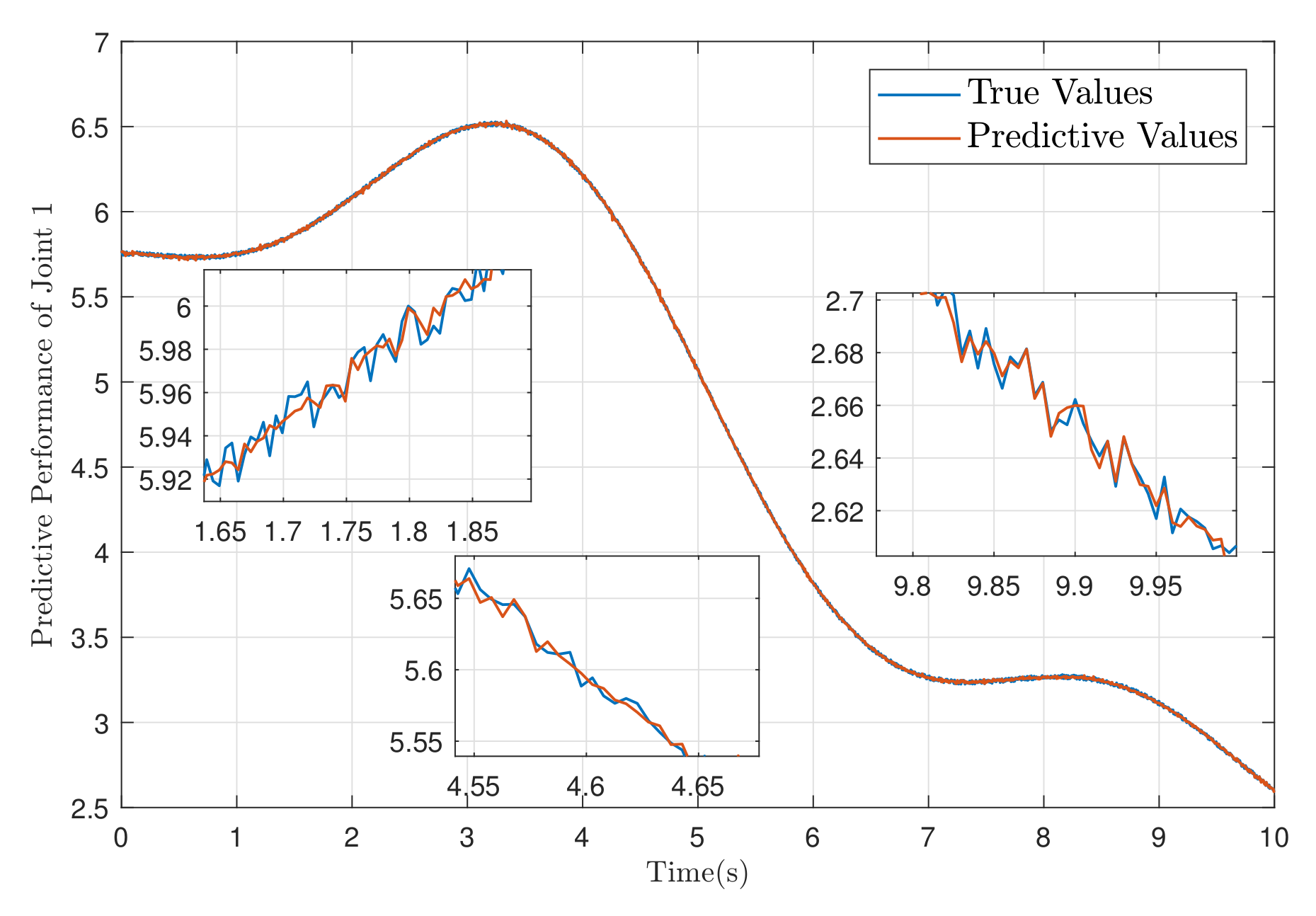
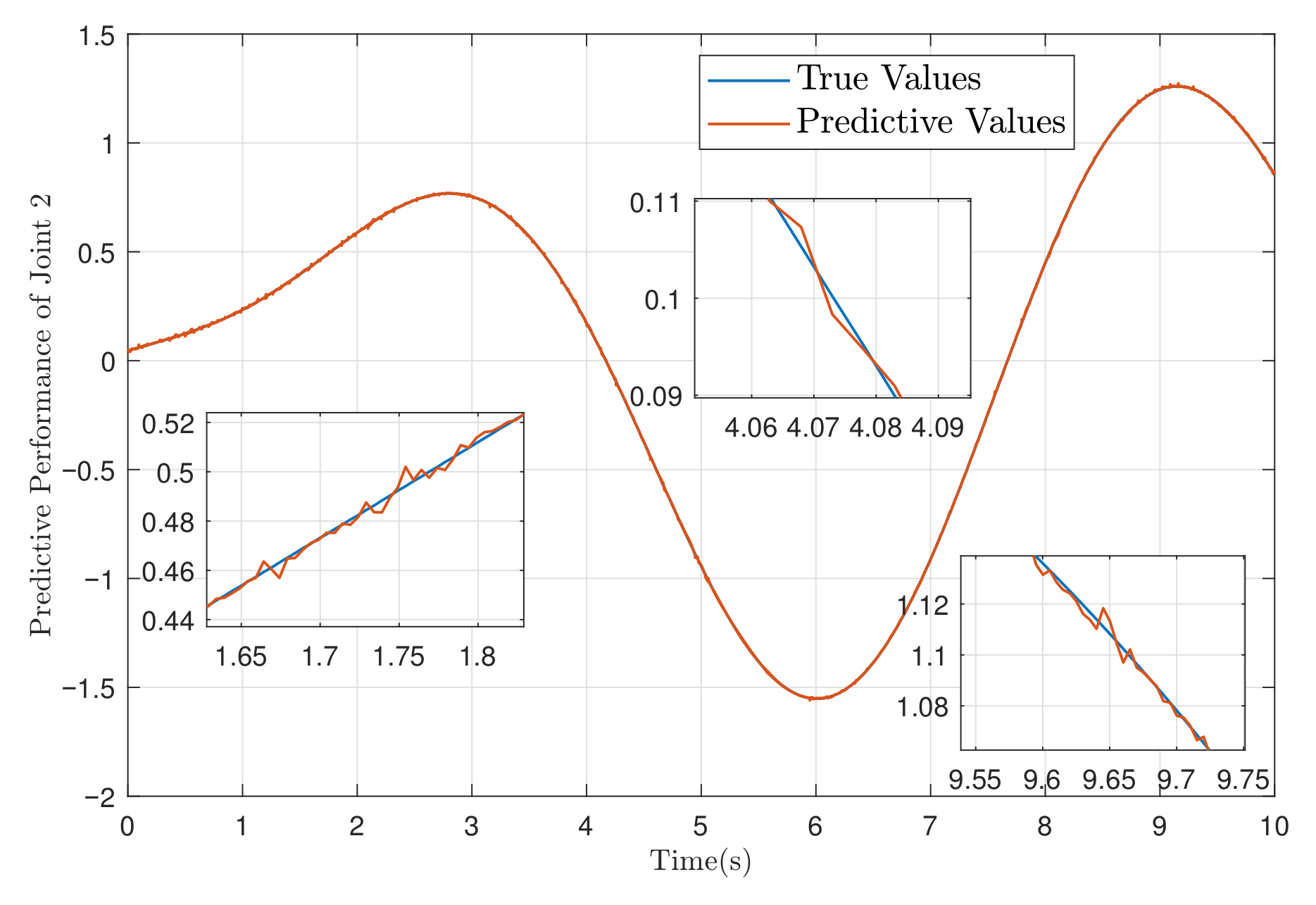
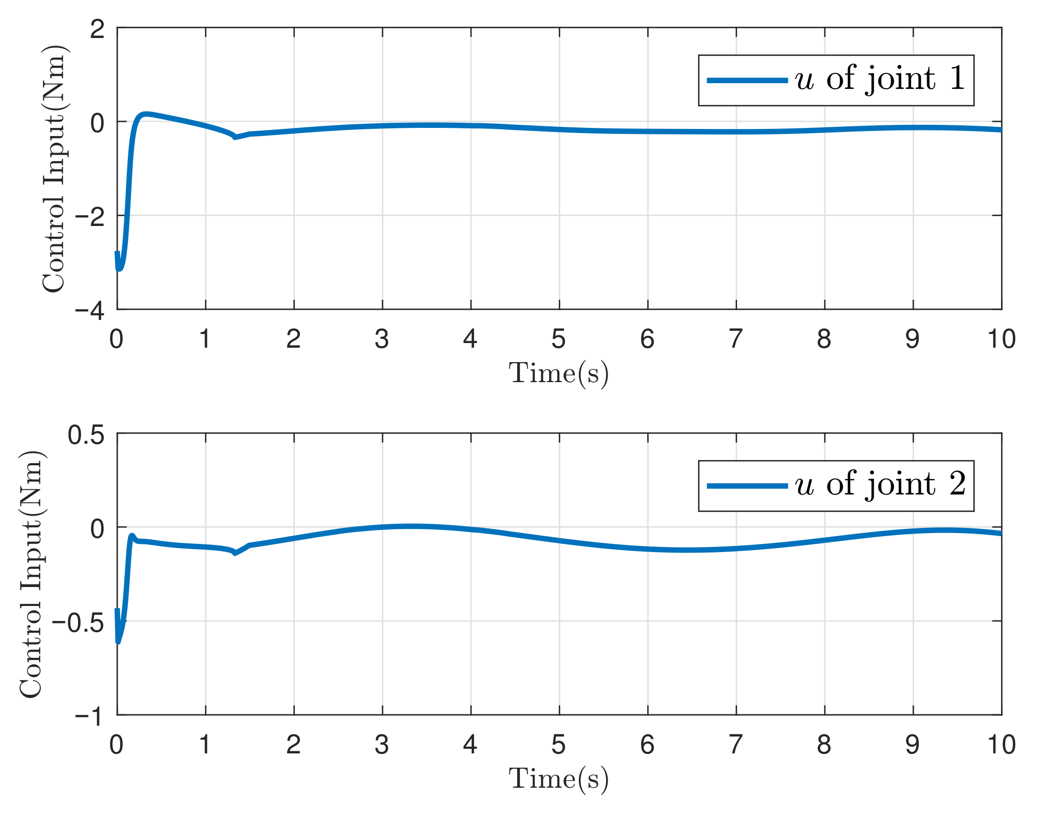
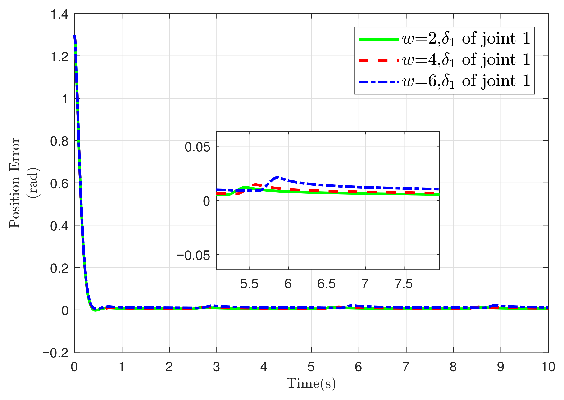
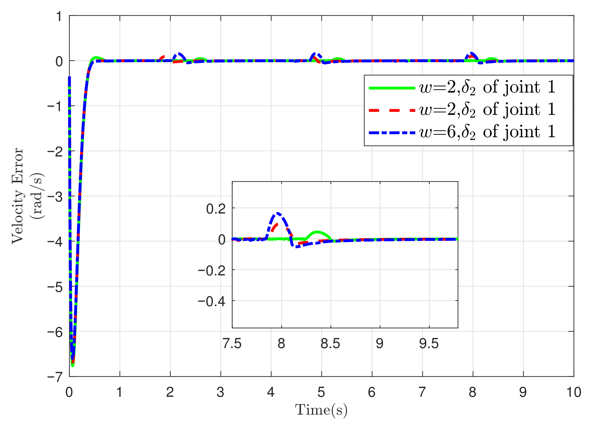
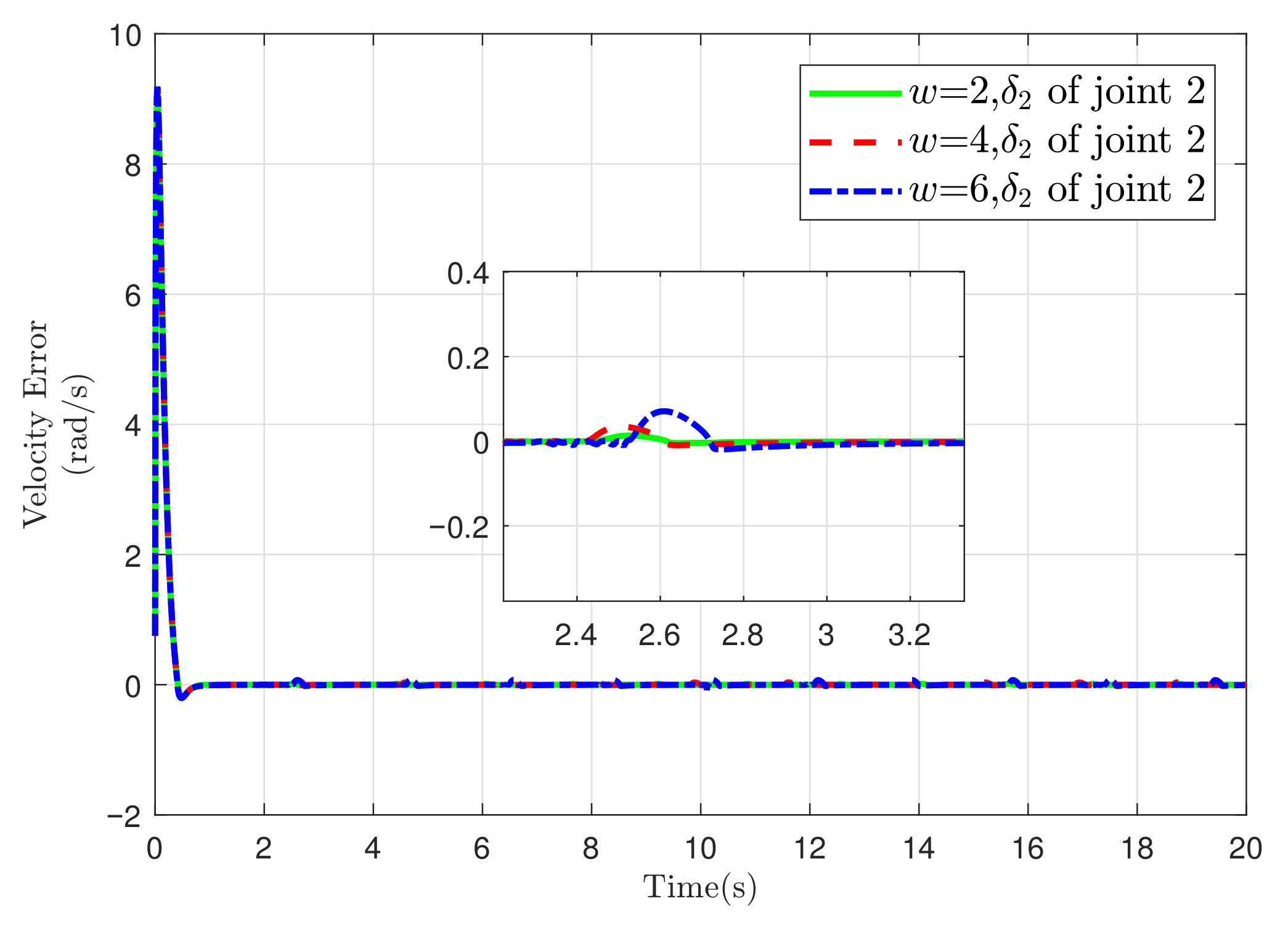
5.2. Simulation of Two-Link Robotic Manipulator

Considering the trajectory tracking issue of a two-link robotic manipulator, we define q 1 and q 2 as the two joint angles of the manipulator. The corresponding items in dynamic Equation (11) of robotic manipulator are denoted as
H ( q ) = H 11 ( q ) H 12 ( q ) H 21 ( q ) H 22 ( q ) , C ( q , q ˙ ) = C 11 ( q , q ˙ ) C 12 ( q , q ˙ ) C 21 ( q , q ˙ ) C 22 ( q , q ˙ ) , g ( q ) = g 1 ( q ) g 2 ( q ) ,
where
H 11 ( q ) = m 1 l c 1 2 + m 2 ( l 1 2 + l c 2 2 ) + 2 m 2 l 1 l 2 cos ( q 2 ) + I 1 + I 2 , H 12 ( q ) = H 21 ( q ) = m 2 l c 2 2 + m 2 l 1 l c 2 cos ( q 2 ) + I 2 , H 22 ( q ) = m 2 l c 2 2 + I 2 , C 11 ( q , q ˙ ) = m 2 l 1 l c 2 sin ( q 2 ) q ˙ 2 , C 12 ( q , q ˙ ) = m 2 l 1 l c 2 sin ( q 2 ) ( q ˙ 1 + q ˙ 2 ) , C 21 ( q , q ˙ ) = m 2 l 1 l c 2 sin ( q 1 ) q ˙ 1 , C 22 ( q , q ˙ ) = 0 , g 1 ( q ) = ( m 1 l c 2 + m 2 l 1 ) g cos ( q 1 ) + m 2 l c 2 g cos ( q 1 + q 2 ) , g 2 ( q ) = m 2 l c 2 g cos ( q 1 + q 2 ) .
The nominal parameters in the above equations are selected as [2] m 1 = 2 ( kg ) , l 1 = 0.35 ( m ) , m 2 = 0.85 ( kg ) , l 2 = 0.31 ( m ) , I 1 = 1 4 m 1 l 1 2 ( kg · m 2 ) , I 2 = 1 4 m 2 l 2 2 ( kg · m 2 ) , and g = 9.81 ( m / s 2 ) . l i is the length of link i, l c i is the distance from link i 1 to the centroid of link i, m i is the mass of link i, and I i is the inertia of link i, ( i = 1 , 2 ) . g is gravitational acceleration. In addition, the external disturbance is u d ( t ) = sin ( t ) + 0.25 sin ( π t ) , 0.5 cos ( 2 t ) + 0.25 sin ( π t ) . Then, the desired trajectory is q d ( t ) = 1.25 7 5 e 0.5 t + 7 20 e t , 1.25 + e 0.5 t + 1 4 e t . The nominal parameters in known dynamics are m 01 = 1.5 ( kg ) , m 02 = 0.5 ( kg ) , l 01 = 0.34 ( m ) , and l 02 = 0.3 ( m ) . The parameters of NFTTSM controller are adjusted as α = β = 3 , p = 0.7 , e = 10 / 9 , r = 6 / 5 , ρ 1 = 1 / 3 , ρ 2 = 6 / 5 , ρ 3 = 3 / 4 , ρ 4 = 2 , ρ 5 = ρ 6 = 2 , D ¯ = 2.3 , and ϵ = 0.01 . According to the conclusions of Theorem 2, the convergence time in (26) is calculated as 17.66 ( s ) .
In the subsequent stage, the GP model learns the truth of the function values of d ( t ) . In this case, we apply the parameters described in the preceding paragraph directly to the robotic manipulator model instead of employing an additional controller. According to Algorithm 1, we generate 1005 homogeneous distributed pairs for GP learning. The acceleration, velocity, and position of joints are collected as q ¨ , q ˙ , q . Then, based on (11), the truth values of u are saved in u . Training data pairs are composed of the values q ¨ , q ˙ , q , and u . These training pairs are used to train the GP and the gradient to optimize the hyperparameters of the squared exponential covariance function. Then, with the target trajectory and feedback gain equal, the proposed controller (25) is applied.
In order to illustrate the superiority of the GP-NFTTSM controller, it is compared with the non-singular terminal sliding-mode controller based on the extended state observer in [2] and the adaptive non-singular fast terminal sliding-mode (ANFTSM) controller in [33]. The control laws in [2,33] are given by (41) and (42), respectively.
u = H 0 ( q ) z 3 + σ γ sig γ 1 ( δ 2 ) + K 1 γ σ diag ( δ 2 ) γ 1 s + ξ + K 2 tanh ( s / ρ 2 ) q ¨ d
where z 3 is the output vector of an extended state observer. The parameters of controller (41) are adjusted as σ = 50 , γ = 1.28 , K 1 = K 2 = diag { 150 , 150 } and ρ = 0.1 .
u = H 0 ( q ) q ¨ d + C 0 ( q ˙ , q ) q ˙ + g 0 ( q ) H 0 ( q ) ξ 1 k 2 ( 1 + ξ 2 k 1 δ 1 ξ 2 1 ) sig 2 ξ 1 ( δ 2 ) H 0 ( q ) [ k s + ( b ^ 0 + b ^ 1 q + b ^ 2 q ˙ 2 + ς ) sign ( s ) ]
where the adaptive laws are b ^ ˙ 0 = λ 0 s δ 2 ξ 2 1 , b ^ ˙ 1 = λ 1 s δ 2 ξ 2 1 q , and b ^ ˙ 2 = λ 2 s δ 2 ξ 2 1 q ˙ 2 . The parameters of controller (42) are selected as ξ 1 = 5 / 3 , ξ 2 = 2 , ς = 0.5 , k 1 = k 2 = 1 , k = 250 and λ 0 = λ 1 = λ 2 = 0.01 . The initial values of b ^ 0 , b ^ 1 and b ^ 2 are set as b ^ 0 ( 0 ) = b ^ 1 ( 0 ) = b ^ 2 ( 0 ) = 0 .
From Figure 10 and Figure 11, we know the proposed GP-NFTTSM controller can realize the convergence of position and velocity tracking errors to 10 4 and 10 3 orders of magnitude respectively in a fixed time with compound disturbance. Compared with the controllers in (41) and (42), the simulations indicate that the proposed control scheme possesses superior capability with regard to fast and high-precision tracking. In the initial phase, the large initial position error leads to a large control input, and from Figure 12 one can obtain that the control input converges to the neighborhood of zero after 1 ( s ) . From Figure 13, one can see that the time responses of sliding-mode variables achieve fast convergence. From Figure 14 and Figure 15, one can conclude that Gaussian process regression can better predict the value of the function d ( t ) in (13) which contains modeling certainties, uncertainties and external disturbances. Compared with Figure 16 and Figure 17, the proposed control scheme has better control performance with smaller control inputs. In addition, the IAE criterion and the ITAE criterion are used to compare the performance of those methods. T p and T v represent the convergence time of position error and velocity error. The results are presented in Table 2. Obviously, the tracking effect of two joints of controller (25) is better than controller (41) and controller (42).
To investigate the effect of model parameters on system performance, we use different parameters for simulation. We can conclude that α , β , r, p, and e all affect the convergence time of the system. From Figure 18, we know that the increases of α and β can reduce the convergence time of the position error. But a value that is too large or too small can cause the amount of state to tremble. Suitable parameter selection can enable the position tracking error δ 1 to converge to the neighborhood of zero within 2 ( s ) and achieve satisfactory tracking performance.
Remark 7.
In the process of the simulation above, we focused on systematically validating the parameters α and β, which have a critical impact on the model, to fully ensure the stability and effectiveness of the proposed control strategy under conditions of parameter variations. For parameters r, p, and e, although no targeted verification experiments were conducted separately in the simulation, during the debugging phase of the overall scheme, their values were repeatedly optimized through multiple sets of comparative tests. Eventually, these parameters were adjusted to the optimal values, as indicated by both theoretical analysis and actual simulation results.
To validate the robustness of the proposed control strategy (25), digital signal disturbances and end-effector load are applied to the system for testing. We define u d ( t ) = [ w i sign ( sin ( 0.05 π t ) ) , w i sign ( sin ( 0.05 π t ) ) ] , ( i = 1 , 2 , 3 ) , where w 1 = 2 , w 2 = 4 , and w 3 = 6 . The load of the end-effector is considered as m l = 1.4 + sin ( t ) . From Figure 19, Figure 20, Figure 21 and Figure 22, one can conclude that under the influence of the load of the end-effector, when the digital signals are switched, the position and velocity tracking errors are affected and produce small fluctuation, but under the action of the proposed controller, the states δ 1 and δ 2 can converge to zero before long.
Conclusions A non-singular terminal sliding-mode controller based on GPR is proposed to guarantee that the tracking errors of uncertain Euler-Lagrange systems converge to a small neighborhood of zero in a fixed time. The non-singular terminal sliding-mode control strategy is used to avert singularity and ensure fast convergence of tracking errors. GPR is utilized to acquire a data-driven offline model. The model parameter uncertainties and external unknown interferences are compensated for by the training results of the model. Simulations demonstrate that the system, using the proposed control strategy, achieves robust tracking of the desired trajectory within a fixed time. The predictive algorithm based on GPR employed in this study demonstrates accurate prediction performance in motion scenarios similar to those of the offline-trained model. Our future efforts will focus on designing an online prediction algorithm to adapt to a broad range of motion scenarios.

Author Contributions

Conceptualization, L.S. and T.L.; methodology, T.L. and T.C.; software, T.L.; validation, T.L. and T.C.; formal analysis, L.S.; investigation, T.L.; resources, L.S.; data curation, T.L.; writing—original draft preparation, T.L. and T.C.; writing—review and editing, L.S.; visualization, T.C.; supervision, L.S.; project administration, L.S.; funding acquisition, L.S. All authors have read and agreed to the published version of the manuscript.

Funding

This research was funded by the National Natural Science Foundation of China (No. 62373038) and the Fundamental Research Funds for the Central Universities (No. FRF-IDRY-GD22-002).

Data Availability Statement

Data are contained within the article.

Conflicts of Interest

The authors declare no conflicts of interest.

References

  1. Yu, X.; Man, Z. Multi-input uncertain linear systems with terminal sliding-mode control. Automatica 1998, 34, 389–392. [Google Scholar] [CrossRef]
  2. Sun, L.; Liu, Y. Extended state observer augmented finite-time trajectory tracking control of uncertain mechanical systems. Mech. Syst. Signal Process. 2020, 139, 106374. [Google Scholar] [CrossRef]
  3. Rouhani, E.; Erfanian, A. A finite-time adaptive fuzzy terminal sliding mode control for uncertain nonlinear systems. Int. J. Control. Autom. Syst. 2018, 16, 1957–1964. [Google Scholar] [CrossRef]
  4. Sun, L.; Zheng, Z. Finite-time sliding mode trajectory tracking control of uncertain mechanical systems. Asian J. Control. 2017, 19, 399–404. [Google Scholar] [CrossRef]
  5. Andrieu, V.; Praly, L. Homogeneous approximation, recursive observer design and output feedback. Siam J. Control. Optim. 2008, 47, 1814–1850. [Google Scholar] [CrossRef]
  6. Polyakov, A. Nonlinear feedback design for fixed-time stabilization of linear control systems. IEEE Trans. Autom. Control. 2012, 57, 2106–2110. [Google Scholar] [CrossRef]
  7. Zuo, Z. Non-singular fixed-time terminal sliding mode control of non-linear system. IET Control Theory Appl. 2015, 9, 545–552. [Google Scholar] [CrossRef]
  8. Zuo, Z.; Tian, B.; Defoort, M.; Ding, Z. Fixed-time consensus tracking for multiagent system with high-order integrator dynamics. IEEE Trans. Autom. Control. 2018, 63, 563–570. [Google Scholar] [CrossRef]
  9. Zuo, Z.; Han, Q.; Ge, X.; Zhang, X. An overview of recent advances in fixed-time cooperative control of multiagent systems. IEEE Trans. Ind. Inform. 2018, 14, 2322–2334. [Google Scholar] [CrossRef]
  10. Cao, S.; Sun, L.; Jiang, J.; Zuo, Z. Reinforcement learning-based fixed-time trajectory tracking control for uncertain robotic manipulators with input saturation. IEEE Trans. Neural Netw. Learn. Syst. 2023, 34, 4584–4595. [Google Scholar] [CrossRef]
  11. Zheng, Y.; Li, Y.; Che, W.; Hou, Z. Adaptive NN-based event-triggered containment control for unknown nonlinear networked systems. IEEE Trans. Neural Netw. Learn. Syst. 2023, 34, 2742–2752. [Google Scholar] [CrossRef] [PubMed]
  12. Chen, C.; Han, Y.; Zhu, S.; Zeng, Z. Neural network-based fixed-time tracking and containment control of second-order heterogeneous nonlinear multiagent systems. IEEE Trans. Neural Netw. Learn. Syst. 2023, 35, 11565–11579. [Google Scholar] [CrossRef] [PubMed]
  13. Xiao, B.; Zhang, H.; Chen, Z.; Cao, L. Fixed-time fault-tolerant optimal attitude control of spacecraft with performance constraint via reinforcement learning. IEEE Trans. Aerosp. Electron. Syst. 2023, 59, 7715–7724. [Google Scholar] [CrossRef]
  14. Williams, C.K.I.; Rasmussen, C.E. Gaussian Processes for Machine Learning; MIT Press: Cambridge, MA, USA, 2006. [Google Scholar]
  15. Deisenroth, M.; Fox, D.; Rasmussen, C. Gaussian processes for data-efficient learning in robotics and control. IEEE Trans. Pattern Anal. Mach. Intell. 2015, 37, 408–423. [Google Scholar] [CrossRef]
  16. Beckers, T.; Umlauft, J.; Kulić, D.; Hirche, S. Stable Gaussian process based tracking control of Euler–Lagrange systems. Automatica 2019, 103, 390–397. [Google Scholar] [CrossRef]
  17. Cen, R.; Jiang, T.; Tang, P. Modified Gaussian process regression based adaptive control for quadrotors. Aerosp. Sci. Technol. 2021, 110, 106483. [Google Scholar] [CrossRef]
  18. Umlauft, J.; Hirche, L. An uncertainly-based control Lyapunov approach for control-affine systems modeled by Gaussian process. IEEE Control Syst. Lett. 2018, 2, 483–488. [Google Scholar] [CrossRef]
  19. Han, F.; Yi, J. Stable learning-based tracking control of underactuated balance robots. IEEE Robot. Autom. Lett. 2021, 6, 1543–1550. [Google Scholar] [CrossRef]
  20. Beckers, T.; Umlauft, J.; Hirche, S. Stable model-based control with Gaussian process regression for robot manipulators. IFAC-PapersOnLine 2017, 50, 3877–3884. [Google Scholar] [CrossRef]
  21. Li, T.; Sun, L.; Jiang, J. Gaussian process-based adaptive sliding mode tracking control for robotic manipulators. In Proceedings of the 2022 WRC Symposium on Advanced Robotics and Automation, Beijing, China, 19 August 2022. [Google Scholar]
  22. Srinivas, N.; Krause, A.; Kakade, S.M.; Seeger, M.W. Information-theoretic regret bounds for Gaussian process optimization in the bandit setting. IEEE Trans. Inf. Theory 2012, 58, 3250–3265. [Google Scholar] [CrossRef]
  23. Bishop, C.M.; Nasrabadi, N.M. Pattern Recognition and Machine Learning; Springer: New York, NY, USA, 2006. [Google Scholar]
  24. Bhat, S.P.; Bernstein, D.S. Finite-time stability of continuous autonomous systems. Siam J. Control Optim. 2000, 38, 751–766. [Google Scholar] [CrossRef]
  25. Zhu, Z.; Xia, Y.; Fu, M. Attitude stabilization of rigid spacecraft with finite-time convergence. Int. J. Robust Nonlinear Control 2011, 21, 686–702. [Google Scholar] [CrossRef]
  26. Zuo, Z. Nonsingular fixed-time consensus tracking for second-order multi-agent networks. Automatica 2015, 54, 305–309. [Google Scholar] [CrossRef]
  27. Huang, Y.; Jia, Y. Fixed-time consensus tracking control for second-order multi-agent systems with bounded input uncertainties via NFFTSM. IET Control Theory Appl. 2017, 11, 2900–2909. [Google Scholar] [CrossRef]
  28. Ravichandran, T.; Wang, D.W.L.; Heppler, G.R. Stability and robustness of a class of nonlinear controllers for robot manipulators. In Proceedings of the 2004 American Control Conference, Boston, MA, USA, 30 June 2004. [Google Scholar]
  29. Jiang, B.; Hu, Q.; Friswell, M.I. Fixed-time rendezvous control of spacecraft with a tumbling target under loss of actuator effectiveness. IEEE Trans. Aerosp. Electron. Syst. 2016, 52, 1576–1586. [Google Scholar] [CrossRef]
  30. Deng, Y.; Wang, X. Terminal sliding-mode controllers for spacecraft-integrated attitude and position motion using the power of twistors. IEEE Trans. Aerosp. Electron. Syst. 2023, 59, 8502–8520. [Google Scholar] [CrossRef]
  31. Liu, Y.; Wang, P.; Lee, C.; Tóth, R. Attitude takeover control for noncooperative space targets based on Gaussian processes with online model learning. IEEE Trans. Aerosp. Electron. Syst. 2024, 60, 3050–3066. [Google Scholar] [CrossRef]
  32. Wang, Q.; Zhou, B.; Duan, G. Robust gain scheduled control of spacecraft rendezvous system subject to input saturation. Aerosp. Sci. Technol. 2015, 42, 442–450. [Google Scholar] [CrossRef]
  33. Boukattaya, M.; Mezghani, N.; Damak, T. Adaptive nonsingular fast terminal sliding-mode control for the tracking problem of uncertain dynamical systems. ISA Trans. 2018, 77, 1–19. [Google Scholar] [CrossRef]
Figure 1. Structure of the proposed closed-loop controller.
Actuators 14 00349 g001
Figure 2. Position error of x and z by (25), u w G P R , and PID.
Actuators 14 00349 g002
Figure 3. Velocity error of x and z by (25), u w G P R , and PID.
Actuators 14 00349 g003
Figure 4. Position error of y by (25), u w G P R , and PID.
Actuators 14 00349 g004
Figure 5. Velocity error of y by (25), u w G P R , and PID.
Actuators 14 00349 g005
Figure 6. Control input of x, y, and z by (25).
Actuators 14 00349 g006
Figure 7. Lumped-disturbance predictive performance of x.
Actuators 14 00349 g007
Figure 8. Lumped-disturbance predictive performance of y.
Actuators 14 00349 g008
Figure 9. Lumped-disturbance predictive performance of z.
Actuators 14 00349 g009
Figure 10. Position error of joint 1 and joint 2 by (25), (41), and (42).
Actuators 14 00349 g010
Figure 11. Velocity error of joint 1 and joint 2 by (25), (41), and (42).
Actuators 14 00349 g011
Figure 12. Control input of joint 1 and joint 2 by (25).
Actuators 14 00349 g012
Figure 13. The value of sliding-mode variable of joint 1 and joint 2 by (25).
Actuators 14 00349 g013
Figure 14. Lumped-disturbance predictive performance of joint 1.
Actuators 14 00349 g014
Figure 15. Lumped-disturbance predictive performance of joint 2.
Actuators 14 00349 g015
Figure 16. Control input of joint 1 and joint 2 by (41).
Actuators 14 00349 g016
Figure 17. Control input of joint 1 and joint 2 by (42).
Actuators 14 00349 g017
Figure 18. Position error of joint 1 and joint 2 with different α and β by (25).
Actuators 14 00349 g018
Figure 19. Position error of joint 1 with compound disturbances and variable load by (25).
Actuators 14 00349 g019
Figure 20. Position error of joint 2 with compound disturbances and variable load by (25).
Actuators 14 00349 g020
Figure 21. Velocity error of joint 1 with compound disturbances and variable load by (25).
Actuators 14 00349 g021
Figure 22. Velocity error of joint 2 with compound disturbances and variable load by (25).
Actuators 14 00349 g022
Table 1. Performance comparisons between those methods.
ControllerController (25)Controller u wGPR Controller PID
x y z x y z x y z
IAE758.9506.3393.41.1  × 10 3 779.5610.51.9  × 10 3 1.4  × 10 3 1.2  × 10 3
ITAE6.1  × 10 3 3.8  × 10 3 3.0  × 10 3 1.4  × 10 4 9.2  × 10 3 7.5  × 10 3 × 10 4 × 10 4 2.5  × 10 4
T p /(s)58.365.259.072.784.5075.4120.4125.3120.4
T v /(s)125.6145.8123.5134.4143.8136.4143.5146.7142.8
e /(rad)0.0620.1220.245
Table 2. Performance comparisons between those methods.
ControllerGP-NFTTSMController (41)Controller (42)
Joint 1 Joint 2 Joint 1 Joint 2 Joint 1 Joint 2
IAE0.11920.13570.15670.16240.48190.5632
ITAE0.11770.04850.12680.10430.49000.3798
T p /(s)0.780.750.920.884.102.10
T v /(s)0.810.800.960.914.502.20
Disclaimer/Publisher’s Note: The statements, opinions and data contained in all publications are solely those of the individual author(s) and contributor(s) and not of MDPI and/or the editor(s). MDPI and/or the editor(s) disclaim responsibility for any injury to people or property resulting from any ideas, methods, instructions or products referred to in the content.

