Analysis of Anchoring Muscles for Pipe Crawling Robots ^†

Abstract

Pneumatic artificial muscles (PAMs) consist of an elastomeric bladder wrapped in a Kevlar braid. When inflated, PAMs expand radially and contract axially, producing large axial forces. PAMs are often utilized for their high specific work and specific power, as well as their ability to produce large axial displacements. Although the axial behavior of PAMs is well studied, the radial behavior has remained underutilized and is poorly understood. Modeling was performed using a force balance approach to capture the effects that bladder strain and applied axial load have on the anchoring force. Radial expansion testing was performed to validate the model. Force due to anchoring was recorded using force transducers attached to sections of aluminum pipe using an MTS servo-hydraulic testing machine. Data from the test were compared to the predicted anchoring force. Radial expansion in large-diameter (over 50.8 mm) PAMs was then used in worm-like robots to create anchoring forces that allow for a peristaltic wave, which creates locomotion through acrylic pipes. By radially expanding, the PAM presses itself into the pipe, creating an anchor point. The previously anchored PAM then deflates, which propels the robot forward. Modeling of the radial expansion forces and anchoring was necessary to determine the pressurization required for proper anchoring before slipping occurs due to the combined robot and payload weight.

1. Introduction

A pneumatic artificial muscle (PAM) is an actuator composed of a braided sleeve wrapped around an elastomeric tube or bladder, which is typically made from latex or silicone. When inflated with a working fluid, the PAM contracts and creates an actuation force, while the diameter of the PAM increases. The force that can be generated by a PAM is a function of the diameter and braid angle of the PAM [1]. PAMs have been found to be extremely useful for producing high-strength forces in low-mass actuators at relatively low pressures, allowing for maximization of specific power, specific work, and power density [2,3,4,5,6,7].

Typically, the force produced by the axial contraction of PAMs is utilized to create actuation of systems [4,8,9,10], but force is also generated by the PAM through the radial expansion that occurs while the PAM axially contracts. Much like with the contractile force, a constraint limiting the ability of the PAM to expand radially must be present for a reaction force to be generated, such as the inner walls of a pipe. While axial contraction force production in PAMs is well understood and various analyses exist to predict these forces [11,12,13,14,15,16], this is not the case for radial force production, and no existing analysis can predict radial force at a given diameter and pressure. This study develops an analysis to predict the radial force generated by a PAM constrained in a tube or pipe and validates the analysis via experiment [17]. The radial force model is then implemented in a pipe-crawling robot. While various crawling robots have been designed before, such as a near-infrared driven soft robot or a tensegrity-based pipe-crawling robot [18,19], the radial force model of the PAM allows for the first pipe-crawling robot constructed from PAMs.

2. PAM Design

A PAM is comprised of three main components: the bladder, the braided sheath, and the end fittings. For the PAM used in this paper, a 57.15 mm (2.25 inch) outer diameter, 6.35 mm (0.25 inch) thick gum rubber bladder (McMaster-Carr, Princeton, NJ, USA) was used with a Kevlar braid (Soller Composites, Franklin, NH, USA). The aluminum end fittings hold the braid and bladder in place by use of a swage tube, which is compressed around it. The end fitting uses a novel two-part design that allows for access to the internals of the PAM without removing the end fitting and destroying the swaged outer tube, shown in Figure 1. These end fittings were custom designed and manufactured in-house.

These end fittings allow for the addition or removal of pneumatic feed-through tubes, which are necessary for robotic applications. The outer end fitting is used for the swaging process and contains a collar that allows the PAM to be connected to external features. The internal end fitting features three holes with 6.35 mm (0.25 inch) NPT threads on both ends to allow for up to three pneumatic attachments and feed-through hoses. An o-ring is placed around the groove in the inner end fitting to provide an airtight seal. A retaining ring is used to hold the inner end fitting in place during operation.

PAM Swaging

The swaging process consists of coating the outer end fitting in epoxy and inserting the smaller diameter end into the bladder. The Kevlar braid is then pulled over top of the end fitting-bladder assembly. The swage tube is then pulled over the end fitting assembly, and the entire piece is passed through a tapered die using an 89,000 N (10 ton) press. The die compresses the swage tube around the other components, creating a unified part. The finished PAM is 311.15 mm (12.25 inches) long and 57.15 mm (2.25 inches) in diameter, with a braid angle of 66.35 degrees shown in Figure 2.

3. Axial Contractile Testing

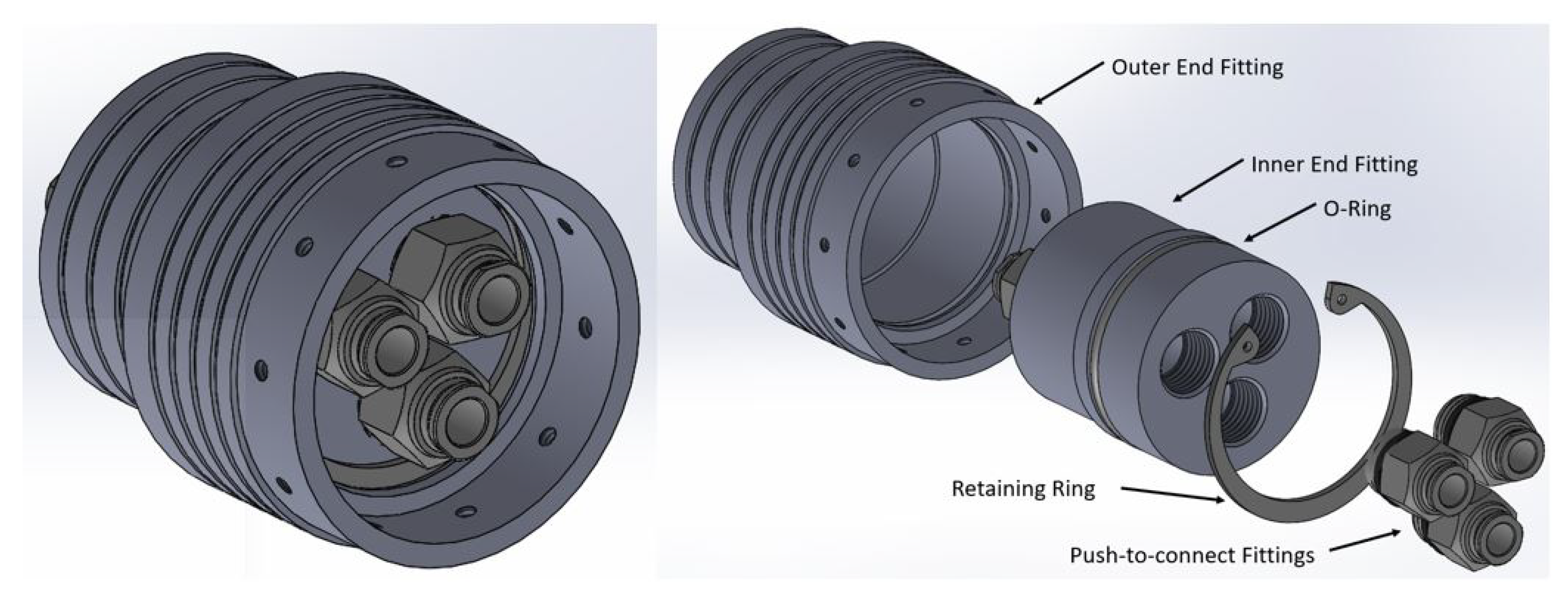
To characterize the radial expansion force of the muscle, first the contractile behavior in the axial direction needed to be modeled to determine key properties such as the axial contractile force output when the muscle is fully elongated, known as the blocked force, the contracted length when no force is applied, known as the free contraction length, and the stresses applied to the bladder. To find these, the PAM was tested on an MTS servohydraulic testing machine. The PAM was connected to the MTS through the use of MTS couplers that were attached to the collars of the end fittings at both ends. The PAM was first manually cycled between free contraction, where the PAM is allowed to fully contract without any applied axial force, and blocked force, where no contraction is allowed and maximum axial force production occurs, at 724 kPa (105 psi) to account for the Mullins effect [20]. The PAM was tested between 69 and 689 kPa (10 and 100 psi) in increments of 69 kPa (10 psi). 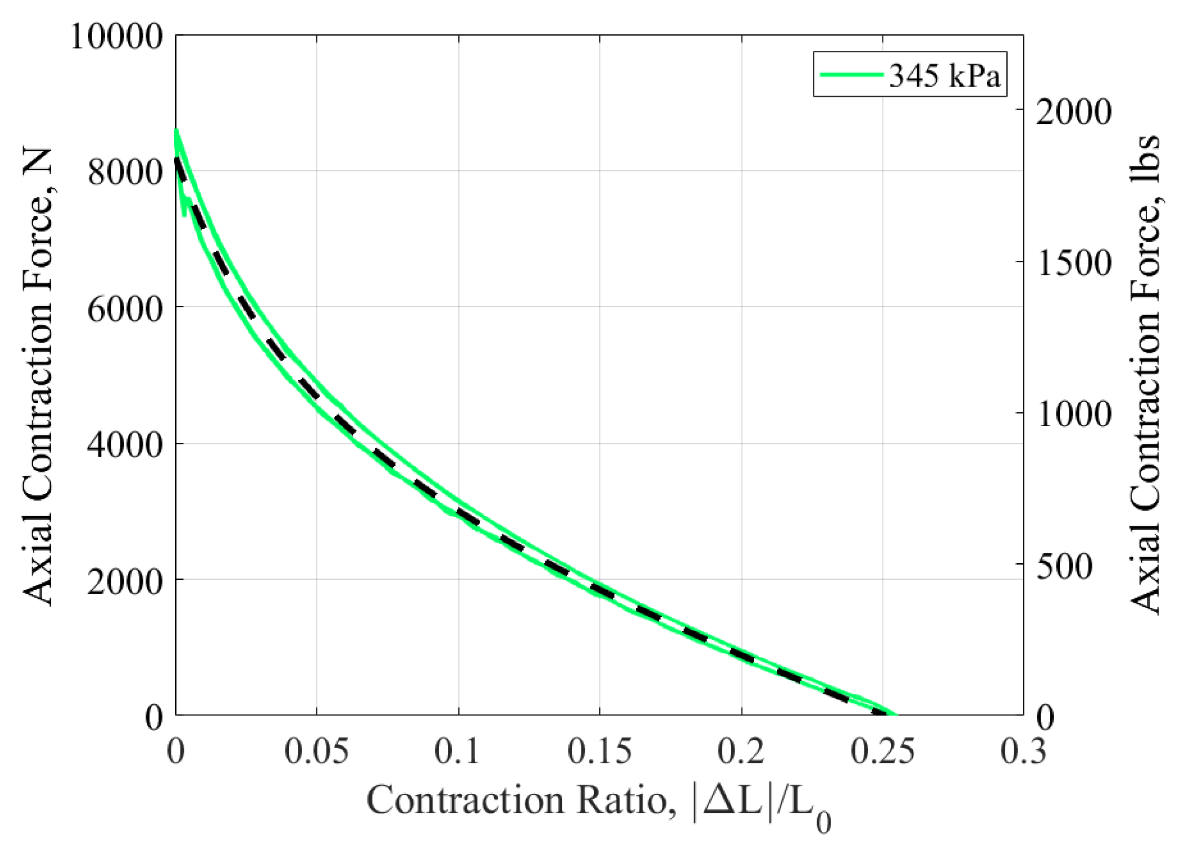For each pressure, the PAM was cycled between blocked force and free contraction three times, as shown in Figure 3. The MTS recorded displacement, force, and pressure. An Enfield D1 Bi-Directional Proportional PWM Valve Driver (Enfield, Trumbull, CT, USA) and an Enfield LS-V05s High Speed 5/3 Proportional Directional Valve (Enfield, Trumbull, CT, USA) were connected to an Arduino Mega (Arduino, Robbinsville, NJ, USA) and used to maintain constant pressure throughout the duration of the experiment. Pressure was measured using an Omegadyne PX209 pressure transducer (Omega Engineering Inc., Norwalk, CT, USA). Due to both the high force output of these muscles and the new end fitting design, precaution was taken at higher pressures to ensure no tearing or separation occurred in the braid or end fittings. No damage was observed during the course of these tests. The data obtained from the axial contraction data of a PAM show a hysteresis effect. The hysteresis is due to a Coulomb frictional force working in opposition to the motion of the PAM [5]. The two legs of the actuation diagram, shown in Figure 4 for the 345 kPa (50 psi) data in green, are averaged together to form a singular actuator load line, represented by the dashed black line. It is this averaged response that is used for the axial contraction modeling.

4. Radial Expansion Testing

To measure the radial force exerted by the muscle, the MTS servohydraulic testing machine was once again used. Two testing fixtures were custom designed to fit into the MTS to allow the MTS to measure the radial force, shown in Figure 5. The testing fixtures consisted of two aluminum half rounds each, with one set measuring 76.2 mm (3 inches) in inner diameter with a 6.25 mm (0.25 inch) wall thickness, and the other measuring 88.9 mm (3.5 inches) in inner diameter with a 6.25 mm (0.25 inch) wall thickness. Mounting fixtures were 3D printed out of ABS using a Makerbot Method X (Makerbot, New York, NY, USA) and epoxied onto the half rounds using Scotchweld DP460 (3M, St. Paul, MN, USA). The two half rounds were placed into the MTS, and the lower head of the MTS was raised until the ends of the half rounds were touching, forming a completed pipe. The PAM was placed in the pipe, and pressure was increased from 69 to 689 kPa (10 to 100 psi) using the same pressure controller described in Section 3. The MTS recorded the force and pressure during the test. Care was taken to ensure proper alignment of the pipe halves and to prevent any separation of the two halves during testing.

5. Axial Contraction Analysis and Results

With the contractile data collected, a model of the PAM could be generated. To generate this model, the braid length, B, and the number of turns of the braid, N, are needed. These can be found using Equations (1) and (2):

$$B={\displaystyle \frac{L_0}{\mathit{sin}\left({\theta }_0\right)}}$$

(1)

$$N={\displaystyle \frac{B\mathit{cos}\left({\theta }_0\right)}{\pi D_0}}$$

(2)

where $L_0$ is the initial active length, ${\theta }_0$ is the initial braid angle, and $D_0$ is the initial diameter. From here, we can find the PAM diameter, D, for any contraction length, as well as the instantaneous braid angle, using the following equations:

$$D\left(L\right)={\displaystyle \frac{\sqrt{B^2-L^2}}{\pi N}}$$

(3)

$${\displaystyle \frac{\mathit{cos}\left({\theta }_1\right)}{D_1}}={\displaystyle \frac{\mathit{cos}\left({\theta }_2\right)}{D_2}}$$

(4)

where L is the current length of the PAM. The force generated by the PAM can now be found using the following equation for the Gaylord force, $F_{\mathit{Gaylord}}$:

$$F_{\mathit{Gaylord}}={\displaystyle \frac{P}{4\pi N^2}}(3L^2-B^2)$$

(5)

where P is the pressure of the working fluid (air) in the PAM. The Gaylord force is most accurate at lower contractions, as it does not account for the energy required to expand the bladder and is therefore less accurate at higher contractions, where bladder expansion is greater [21].

Following the procedures outlined in ref. [22], a characterization of the PAM that incorporates bladder expansion can be determined using the MTS data and the fmincon command in MATLAB version R2024b to determine the non-linear moduli of the bladder [22]. These moduli are allowed to vary linearly with pressure and provide a 4^th-order approximation of the non-linear behavior of the bladder. The axial and circumferential strain, ${ϵ}_z$ and ${ϵ}_c$, can be found using:

$${ϵ}_z={\displaystyle \frac{L}{L_0}}-1$$

(6)

$${ϵ}_c={\displaystyle \frac{R}{R_0}}-1$$

(7)

where R is the instantaneous radius of the bladder, and $R_0$ is the initial radius. The instantaneous axial and circumferential stress in the PAM can then be determined using the strains and the moduli, $E_k$:

$${\sigma }_z=\sum _{k=1}^4{E}_k{ϵ}_z^k$$

(8)

$${\sigma }_c=\sum _{k=1}^4{E}_k{ϵ}_c^k$$

(9)

Finally, the instantaneous force produced by the PAM can be calculated using the force balance model:

$$F=P{R}_i\left({\displaystyle \frac{L^2}{2\pi R_o{N}^2}}-\pi R_i\right)+{\sigma }_z{\displaystyle \frac{V_B}{L}}-{\sigma }_c{\displaystyle \frac{t{L}^2}{2\pi R_o{N}^2}}$$

(10)

where $V_B$ is the volume of the bladder, which is assumed constant for this model, t is the thickness of the bladder, $R_o$ is the outer radius of the PAM, and $R_i$ is the inner radius. Note that due to the non-negligable thickness of the bladder, a distinction was made in the radii terms between the inner and outer radius of the bladder for this model, unlike the model used in ref. [22].

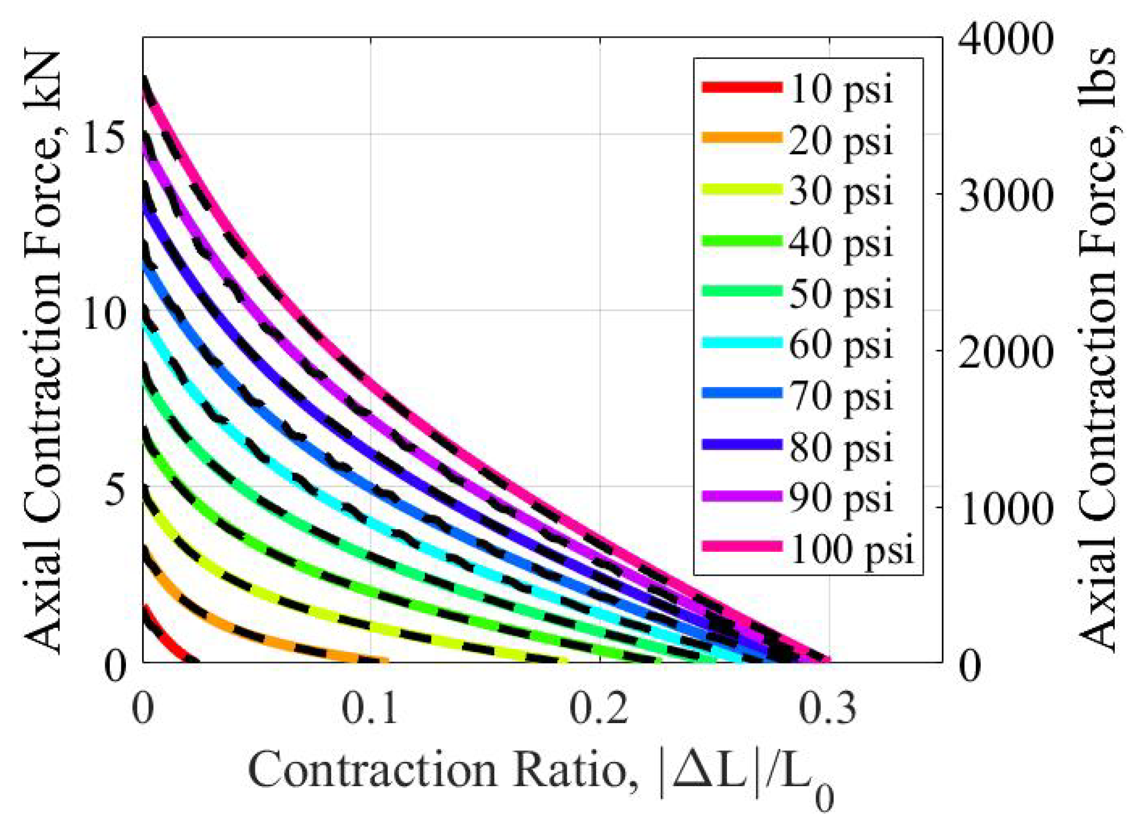
The axial contraction model is comprised of three terms. The first term, $P{R}_i({\displaystyle \frac{L^2}{2\pi R_o{N}^2}}-\pi R_i)$, is equivalent to the Gaylord force from Equation (5). The second and third terms, ${\sigma }_z{\displaystyle \frac{V_B}{L}}-{\sigma }_c{\displaystyle \frac{t{L}^2}{2\pi R_o{N}^2}}$ are the forces resulting from the axial and circumferential stress in the bladder, respectively. These forces act against the Gaylord force and reduce the total force output by the muscle. The results of the analysis are shown in Figure 6. The dashed black lines represent the experimental data obtained from the test described in Section 3, while the colored lines represent the results predicted by the model. The sum of the root mean squared error for each tested pressure was 595.2 N (133.8 lbs).

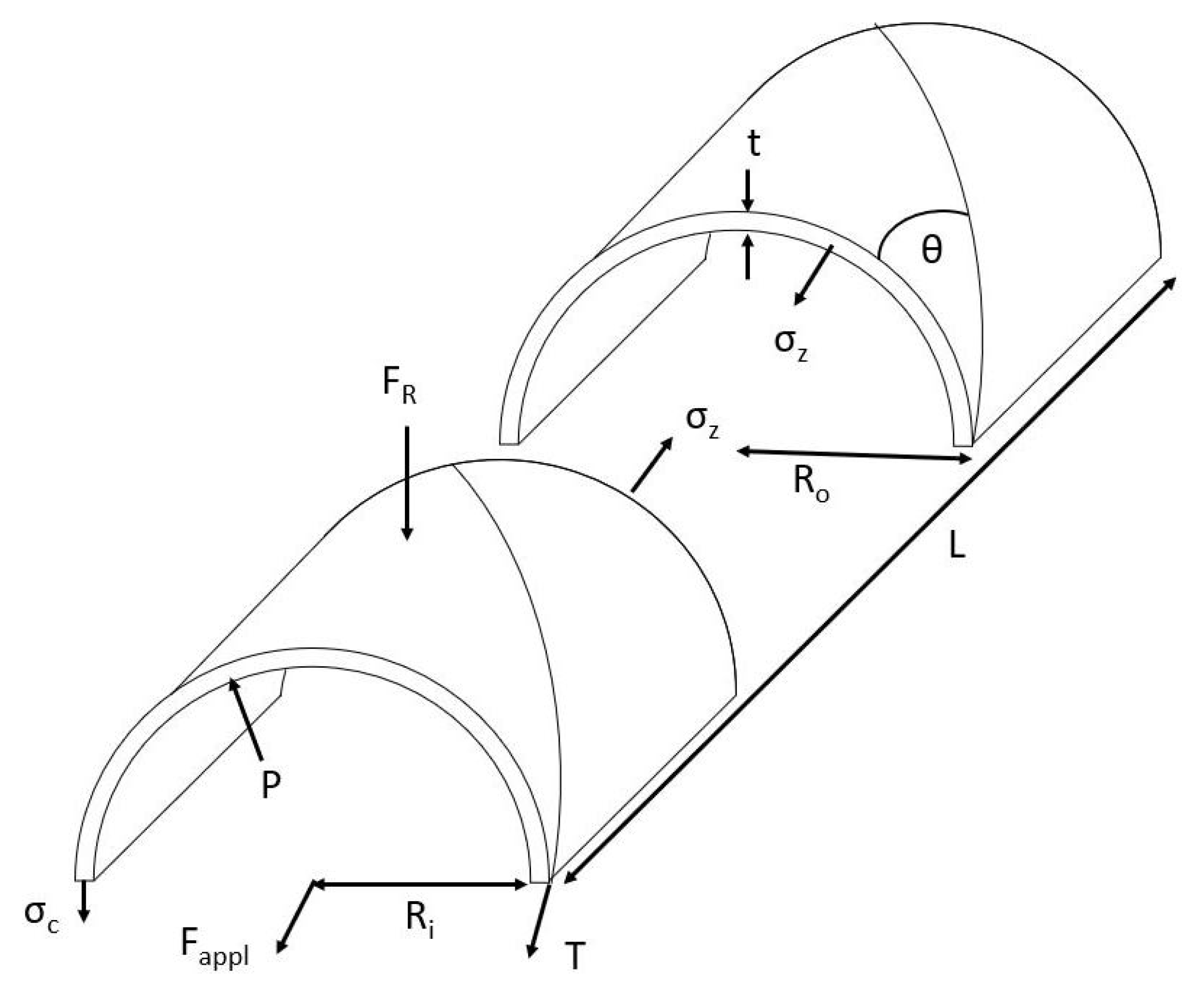
6. Radial Expansion Analysis and Results

Using the free body diagram depicted in Figure 7, the radial expansion force can be modeled. First, balancing the forces in the circumferential and axial directions results in Equations (11) and (12).

$$P{R}_{i}L={\sigma }_{c}tL+NTcos\left(\theta \right)+{\displaystyle \frac{1}{2}}{F}_R$$

(11)

$$F_{\mathit{appl}}+\pi R_i^{2}P={\sigma }_z{\displaystyle \frac{V_B}{L}}+Tsin\left(\theta \right)$$

(12)

where $F_R$ is the radial force generated by the PAM, T is the tension in the braid, pointing along the long axis of the fiber of the braid, and $F_{\mathit{appl}}$ is an applied axial load. By solving Equation (11) for T, Equation (1) for $sin\left(\theta \right)$, and Equation (2) for $cos\left(\theta \right)$ (and substituting), Equation (12) becomes:

$$F_{\mathit{appl}}+\pi R_i^{2}P={\sigma }_z{\displaystyle \frac{V_B}{L}}+{\displaystyle \frac{(P{R}_{i}L-{\sigma }_{c}tL-\frac{1}{2}{F}_R)L}{2\pi R_o{N}^2}}$$

(13)

Equation (13) can then be solved for $F_R$:

$$F_R=2\left[P\left(R_{i}L-{\displaystyle \frac{2{\pi }^2{R}_i^2{R}_o{N}^2}{L}}\right)+2\pi R_o{N}^2{\sigma }_z{\displaystyle \frac{V_B}{L^2}}-{\sigma }_{c}tL-{\displaystyle \frac{2\pi R_o{N}^2{F}_{\mathit{appl}}}{L}}\right]$$

(14)

Equation (14) describes the force applied radially by a PAM to a tube it is contained in for a given pressure and applied axial force. Like the axial contraction force equation, it is beneficial to break down this equation into its constituent parts. The first part, $P(R_{i}L-{\displaystyle \frac{2\pi R_i^2{R}_o{N}^2}{L}})$, describes the force generated by the internal pressure acting on both the walls of the bladder as well as the faces of the end fitting. The second and third terms, $2\pi R_{o}N{\sigma }_z{\displaystyle \frac{V_B}{L^2}}-{\sigma }_{x}tL$, are the forces due to the axial and circumferential stress in the bladder. Much like their function in the axial contraction model, they work to reduce the force produced by the first term. The final section, ${\displaystyle \frac{2\pi R_o{N}^2{F}_{\mathit{appl}}}{L}}$, is the external axial force applied to the PAM. Due to the Kevlar braid, a coupling exists between the circumferential and axial functions of the PAM. This results in a reduction of circumferential force production as axial loading is applied to the muscle. An alternative formulation to Equation (14) would be to express the radial expansion in terms of force per length, as in Equation (15):

$${\displaystyle \frac{F_R}{L}}=2\left[P\left(R_i-{\displaystyle \frac{2{\pi }^2{R}_i^2{R}_o{N}^2}{L^2}}\right)+2\pi R_o{N}^2{\sigma }_z{\displaystyle \frac{V_B}{L^3}}-{\sigma }_{c}t-{\displaystyle \frac{2\pi R_o{N}^2{F}_{\mathit{appl}}}{L^2}}\right]$$

(15)

This formulation is convenient for comparison of PAMs of equal diameter but different length. By normalizing over the length of the muscle, the PAMs can be compared by their output of radial expansion force per length, allowing for a consistent and direct form of comparison. Additionally, by dividing Equation (15) by the circumference of the anchored PAM, the pressure applied to the pipe by the PAM can be found, which is useful when anchoring in materials where applying too much pressure could disrupt the tunnel, such as tunnels made of gravel or sand.

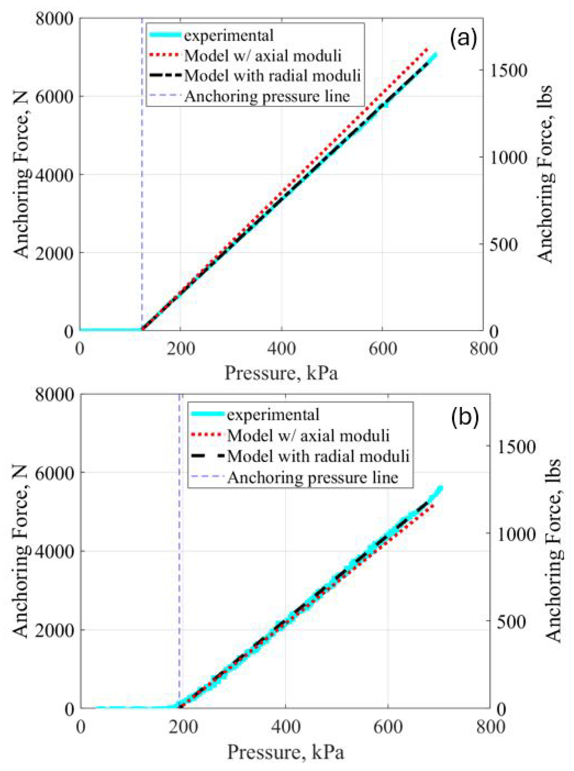
The radial expansion model was compared to the data obtained from the radial MTS tests. The moduli obtained from the axial model were used for the radial model initially. Though the model correctly predicted when anchoring would occur, the model was not accurate when using the moduli from the axial expansion model above anchoring pressure, as seen in Figure 8. The root mean squared error for the 76.2 mm (3 inch) and 88.9 mm (3.5 inch) diameter cases were found to be 206.57 and 105.06 N (46.44 and 23.62 lbs), respectively. Here, anchoring pressure is defined as the pressure where the PAM first contacts the pipe wall and anchoring begins. Anchoring occurs to the right of the vertical dashed blue line.

Optimization was performed on the model using the radial expansion data to find new moduli.

$$\begin{array}{cc}\hfill \underset{x}{\min }& \sum _{k=1}^n\sqrt{{\displaystyle \frac{{\sum }_{i=1}^m{(F_{M,i,k}-F_{E,i,k})}^2}{m}}}\hfill \\ \hfill \mathrm{s}.\mathrm{t}.& lb\le x\ge ub\hfill \\ \hfill & c\left(x\right)\le 0\hfill \end{array}$$

(16)

Here, $F_M$ is the predicted force from the model, $F_E$ is the measured experimental force, n is the number of pressures tested, and m is the total number of data points per pressure taken. The optimization variable, x, is a vector comprised of ${[x_1,x_2,x_3,x_4,x_5,x_6,x_7,x_8]}^T$. These variables are used to determine the moduli in the form of

$$\begin{array}{ccc}\hfill E_1& =& x_{1}P+x_2\hfill \\ \hfill E_2& =& x_{3}P+x_4\hfill \\ \hfill E_3& =& x_{5}P+x_6\hfill \\ \hfill E_4& =& x_{7}P+x_8\hfill \end{array}$$

(17)

The bounds on x are given by $\left\{x_k=-1000\left|k=1,...,8\right.\right\}$ and $\left\{x_k=1000\left|k=1,...,8\right.\right\}$ as the lower and upper bounds, respectively. Finally, the non-linear constraint, $c\left(x\right)$, can be defined as:

$$c\left(x\right)=-(d{E}_c+d{E}_z)$$

(18)

where $d{E}_c$ is the incremental internal circumferential energy and $d{E}_z$ is the incremental internal axial energy. This constraint is derived from the Drucker stability criteria, which states that the incremental internal energy of a stable material can only increase [23].

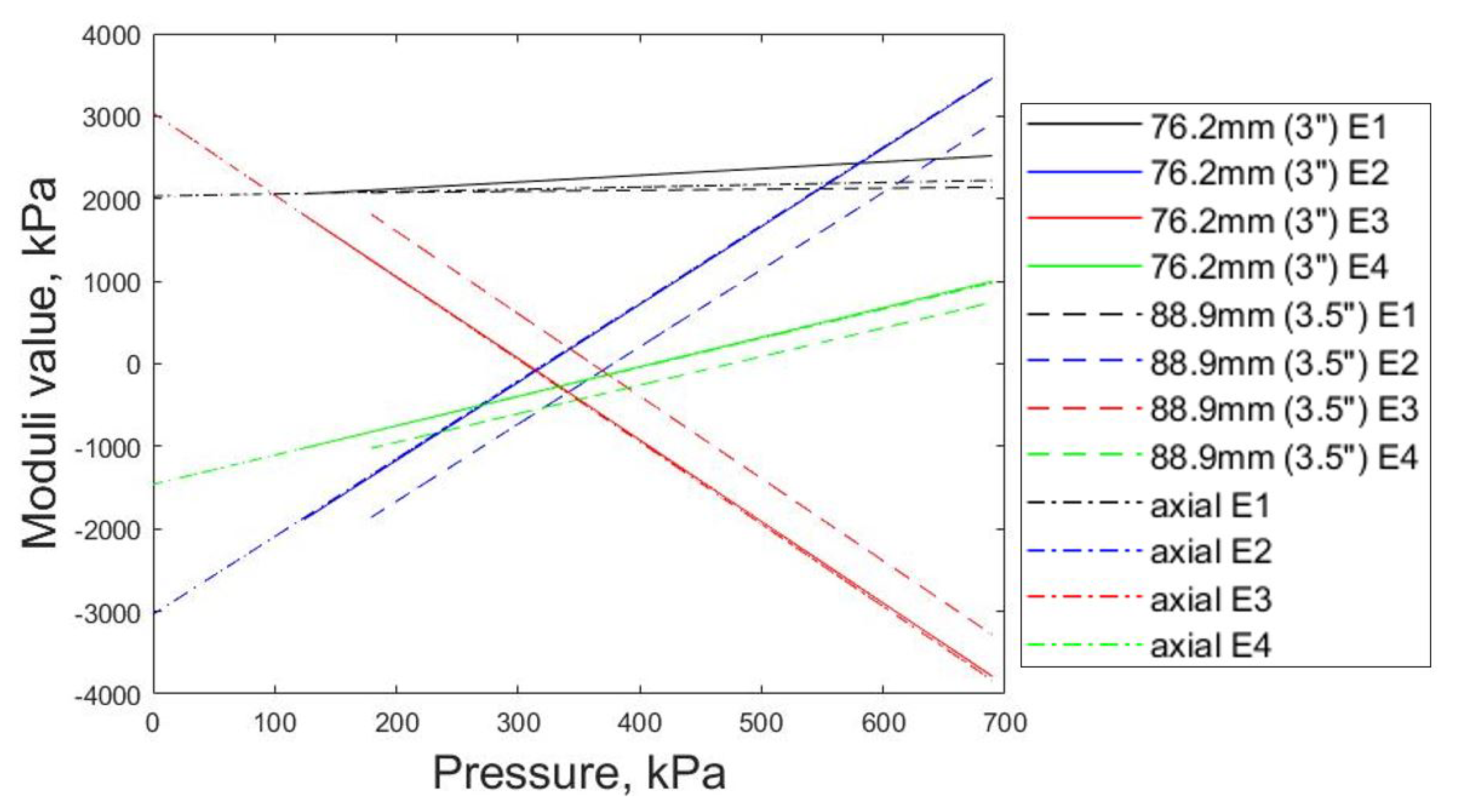
The stress in the bladder was calculated using these new moduli and compared to the stress seen in the axial contraction model for both the 3- and 3.5-inch data sets. The stress was found to be the same at the pressure where contact with the pipe first occurred, called the contact pressure, for both the axial and circumferential stress between the two models for both data sets. As the pressure increased, both the circumferential and axial stress in the radial expansion model changed at different rates than the stresses in the axial contraction model, as seen in Figure 9. There are multiple reasons that could be the cause of the bladder stress not aligning between the two models, such as bladder stiffening due to contact with the pipe, inaccuracies due to an inextensible braid assumption, frictional losses due to braid-bladder contact and braid-pipe contact, or the constant radius assumption that may not hold for the axial contraction model but which would hold for the radial expansion model due to the pipe forcing a constant bladder radius onto the PAM [24]. These reasons could also explain why the moduli found for the two sets of radial data differ, as shown in Figure 10.

The radial expansion model was run once again using these new stress values, shown as the dashed black lines in Figure 8. The model follows the experimental data very well. The root mean squared error for the 76.2 mm (3 inch) and 88.9 mm (3.5 inch) diameter cases were found to be 0.147 and 0.151 N (0.033 and 0.034 lbs), respectively. As expected, the radial force increases linearly as the pressure increases.

Radial Force with Applied Axial Load

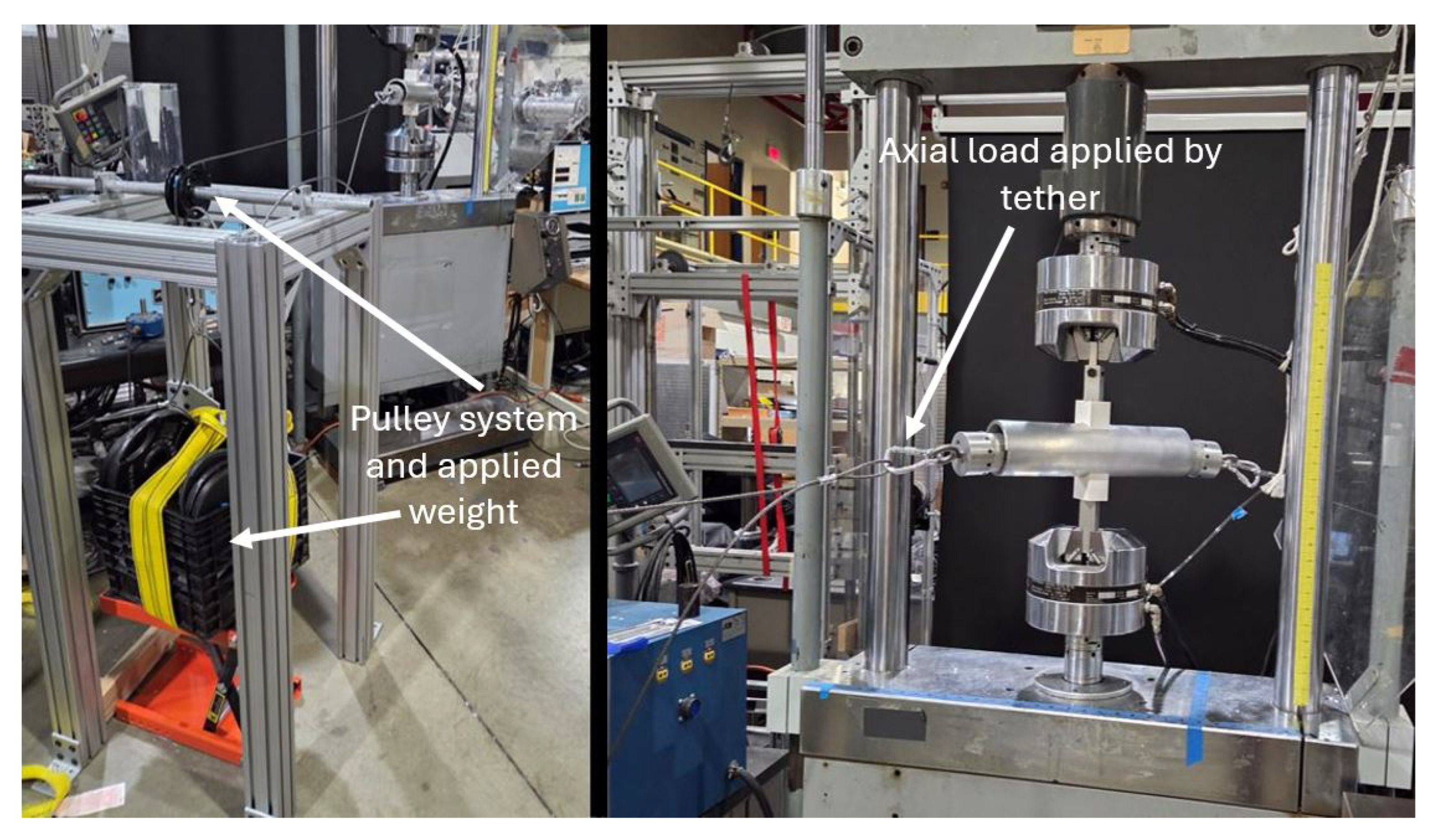
While we have validated the radial force model against data, this data was collected under the condition that no axial force was applied to the PAM during the test. As noted earlier, the final term in Equation (14) represents how an applied axial force would affect the radial force, and up to now, this term has not been validated. An additional test was performed for each test fixture, where a rope was attached to one end of the PAM. The rope was run through a pulley, and a crate containing 1024.74 N (230.37 lbs) of weight was hung from the opposing end, as shown in Figure 11. The PAM was once again inflated from 69 to 689 kPa (10 to 100 psi), and the produced radial force was recorded. A new PAM was used for these tests. The PAM was 57.15 mm (2.25 inches) in diameter with a length of 314.325 mm (12.375 inches) and a braid angle of 65.92 degrees.

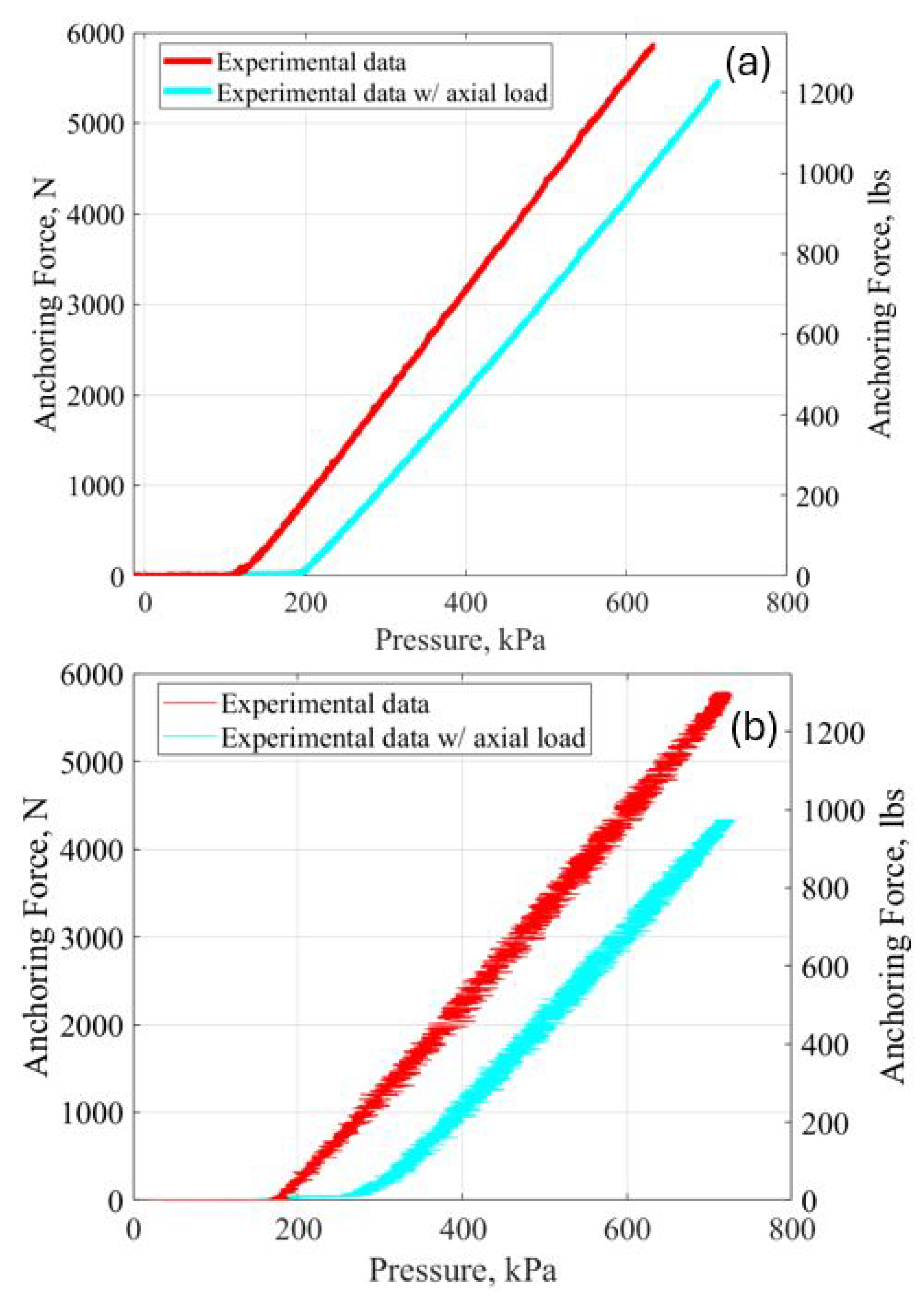
Figure 12 shows the results of the data from the 76.2 mm (3 inch) and 88.9 mm (3.5 inch) diameter case compared to the data for each respective case with no axial loading applied. The load was measured using an ACCUTEK ShipPro scale (Amazon, Seattle, WA, USA), which had an accuracy of 0.003 kg. For our load of 1024.74 N (230.37 lbs), we see a reduction of 1039.64 N (233.72 lbs) for the 76.2 mm (3 inch) diameter case and 1316.98 N (296.07 lbs) for the 88.9 mm (3.5 inch) diameter case. In both cases, we observed that the anchoring pressure of the PAM has shifted to the right, but the slope of the curve remains relatively the same between the case with the applied axial force and the case without. This agrees with Equation (14), where the applied axial term, ${\displaystyle \frac{4\pi R_0{N}^2{F}_{\mathit{appl}}}{L}}$ acts to reduce $F_R$ as $F_{\mathit{appl}}$ increases, creating a shift to the right on the x-axis. 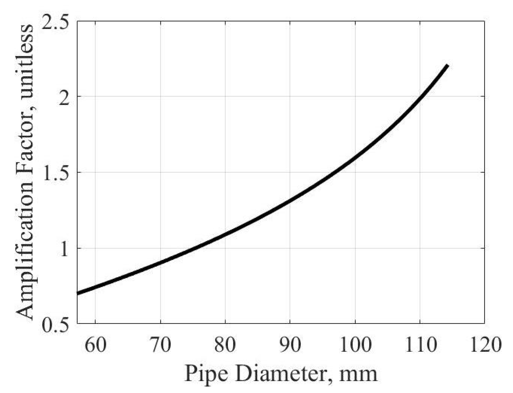The nondimensional ratio, ${\displaystyle \frac{4\pi R_0{N}^2}{L}}$, can be viewed as a nondimensional amplification factor. This term increases or decreases the applied force depending on the diameter of the pipe and length of the PAM, causing the effective force reduction to amplify as the pipe diameter increases. Figure 13 shows the change in the amplification factor as pipe diameter increases.

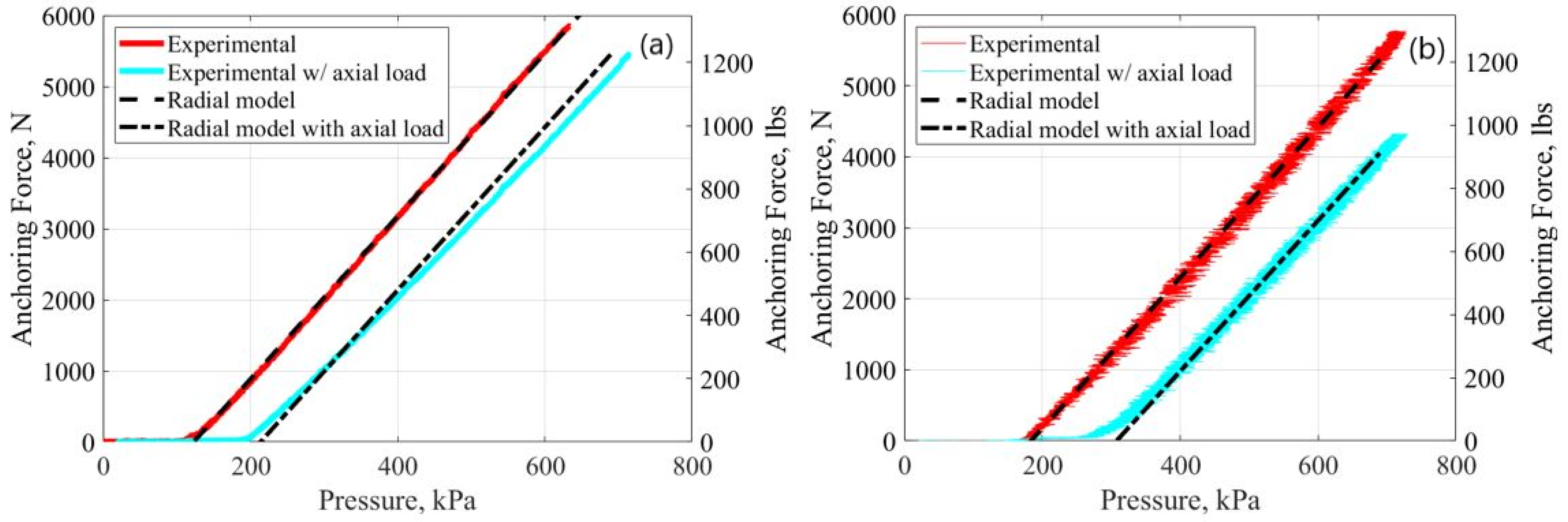
Figure 14 shows the fitted model against the raw data for both cases. Here, the model was fitted to the data without the applied axial load using the optimization function described previously. The term for the applied axial load was then added to the model, without running the optimization function again, and overlaid overtop the data with the applied axial load. The model accurately accounts for the shift that occurs with the application of an axial load, with no need to obtain new moduli through optimization. The root mean squared errors for the 76.2 mm (3 inch) and 88.9 mm (3.5 inch) cases are 174.46 and 76.11 N (39.22 and 17.11 lbs), respectively. While relatively low, these errors are higher than the errors seen for the model without the applied axial load. This phenomenon may occur due to certain assumptions in the model that are not accounted for, such as friction and hysteresis.

The oscillatory behavior seen in the 88.9 mm (3.5 inch) case is due to the behavior of both the PID controller used to control the pressure of the PAM, along with the controller used by the MTS to keep the two halves of the pipe in place during the radial actuation of the PAM. While the PID pressure controller was tuned to work well with the 76.2 mm (3 inch) case, it struggled to hold pressure as well for the 88.9 mm (3.5 inch) case due to the larger bladder volume, requiring the system to control a higher volume of air at a given pressure. The MTS controller struggled to keep the lower half of the pipe in place and would overshoot the set position, also causing the recorded force to fluctuate. The variation in the pressure due to noise is about 27.6 to 34.5 kPa (4 to 5 psi). Although additional noise exists in this case, it can be seen that the radial model follows the averaged trend line of the data well.

7. Model Compatibility

As shown in Section 6, the stresses present in the bladder differ in the muscle when the muscle is constrained in a pipe versus when it is not. Despite this, both the axial and circumferential stresses in the bladder at the time of anchoring are equal between the two models. This allows for compatibility between the axial contraction and radial expansion model. While the muscle is free to expand radially, the axial contraction model accurately describes the muscle behavior. Once contact with the pipe wall is established, the radial model and moduli should be used while the PAM is anchored. The pressure where the switch between models should occur is the same as the anchoring pressure. This pressure can be found by solving Equation (3) for the length, using the desired inner diameter of the pipe. This length can then be compared to a pressure versus free contraction plot that is obtained from the axial contraction data, as in Figure 15. For an inner pipe diameter of 76.2 mm (3 inch), anchoring occurs at a free contraction length of 286.77 mm (11.29 inches) for the PAM used in the radial testing without axial loading, which corresponds to a pressure of $P_a$(3″) = 117 kPa (17 psi). Anchoring occurs at a free contraction length of 265.43 mm (10.45 inches) for a pipe diameter of 88.9 mm (3.5 inch), which corresponds to a pressure of $P_a$(3.5″) = 165 kPa (24 psi), as shown in Figure 15, which agrees with the experimental data.

8. Robotic Applications

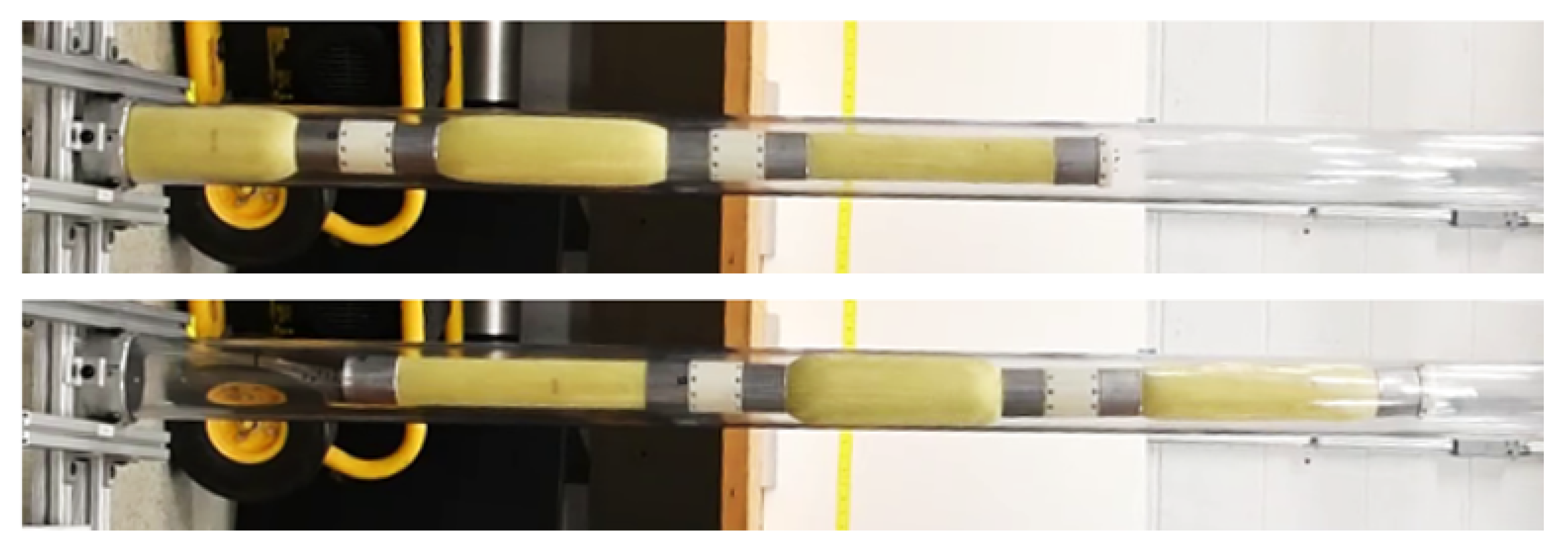
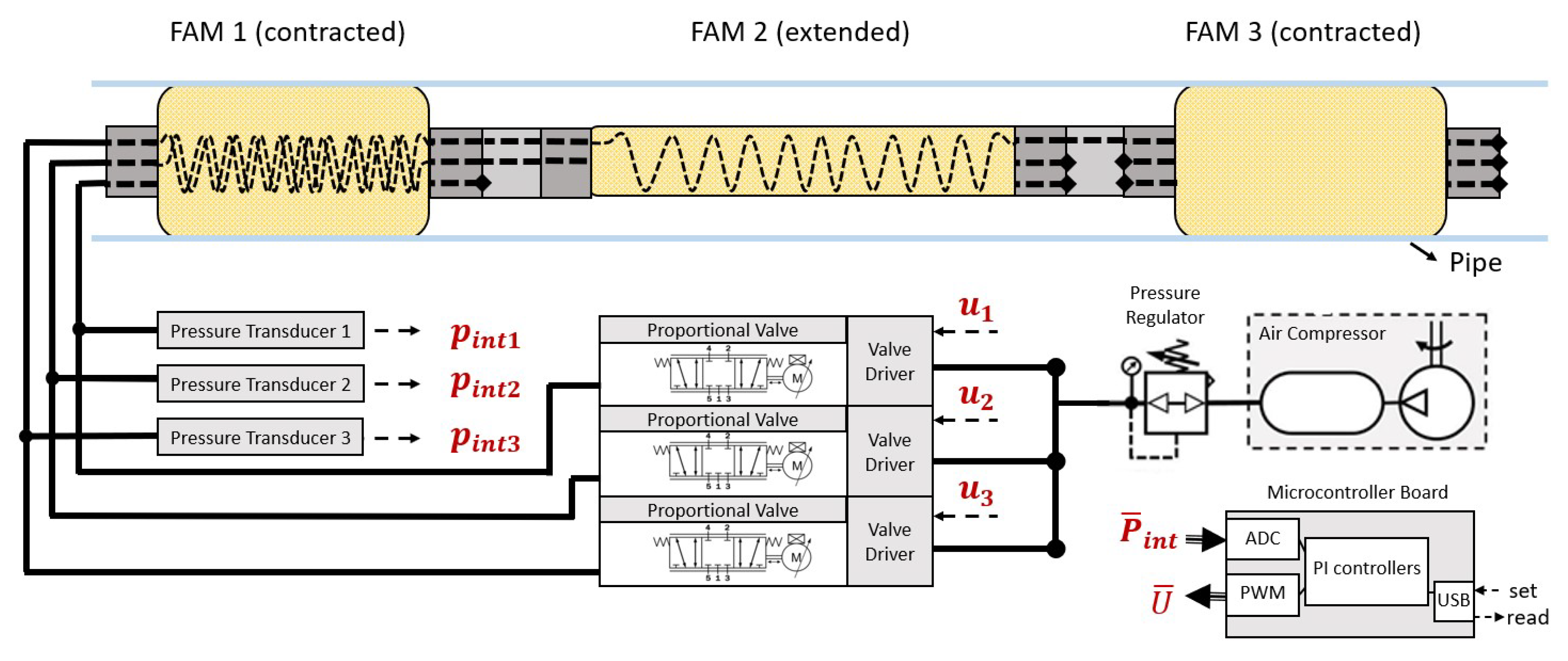
With a functioning radial model developed, a soft robot capable of utilizing the radial expansion force of a PAM was developed. When combined axially, three PAMs can be linked to form a single worm-like robot capable of movement through tunnels and pipes, such as in Figure 16, where a three-segment PAM robot starts at the bottom of a vertical pipe and ascends. Using a system of internal pneumatic tubing, each PAM can be individually pressurized and monitored, as shown in Figure 17.

Through the use of this electro-pneumatic system, the robot moves through a pipe using a pattern of inflation and deflation, (shown in Figure 18, akin to that of a peristaltic wave used by worms when tunneling) [25].

The gait initiates in Step I with the middle PAM, or PAM2, which is inflated and anchored to the pipe wall and acts as a fixed point for the robot. In Step I, PAM2 assumes the role of the anchor PAM. Here, the center of mass of PAM2 also serves as the reference for forward locomotion. In Step II, the rear-most PAM1 contracts and anchors to the pipe wall, so that PAM1 assumes the anchor PAM role. In Step III, with the rear-most PAM1 anchored, PAM2 deflates and elongates. In Step IV, the peristaltic wave continues to propagate as the forward-most PAM3 assumes the anchor PAM role, and anchors to the pipe wall. In Step V, the rear-most PAM1 deflates, and no longer anchors. In step VI, the middle PAM inflates, moving its center of mass forward, and PAM2 again assumes the anchor PAM role. In Step VII, the forward-most PAM3 deflates so that the front end of the robot moves forward. The robot is now in the same state as Step I, but the center of mass of PAM2 has made forward progress. The cycle then re-starts. For this locomotion method to work while climbing an inclined pipe, the force provided by the anchoring muscle must be able to counteract the weight of the robot and any additional payload so slipping does not occur. The ability to predict the anchoring force provided by the robot given the pressure supplied to the PAM through the use of the radial expansion model is crucial to ensure sufficient anchoring force, so that loss of anchoring does not occur during locomotion.

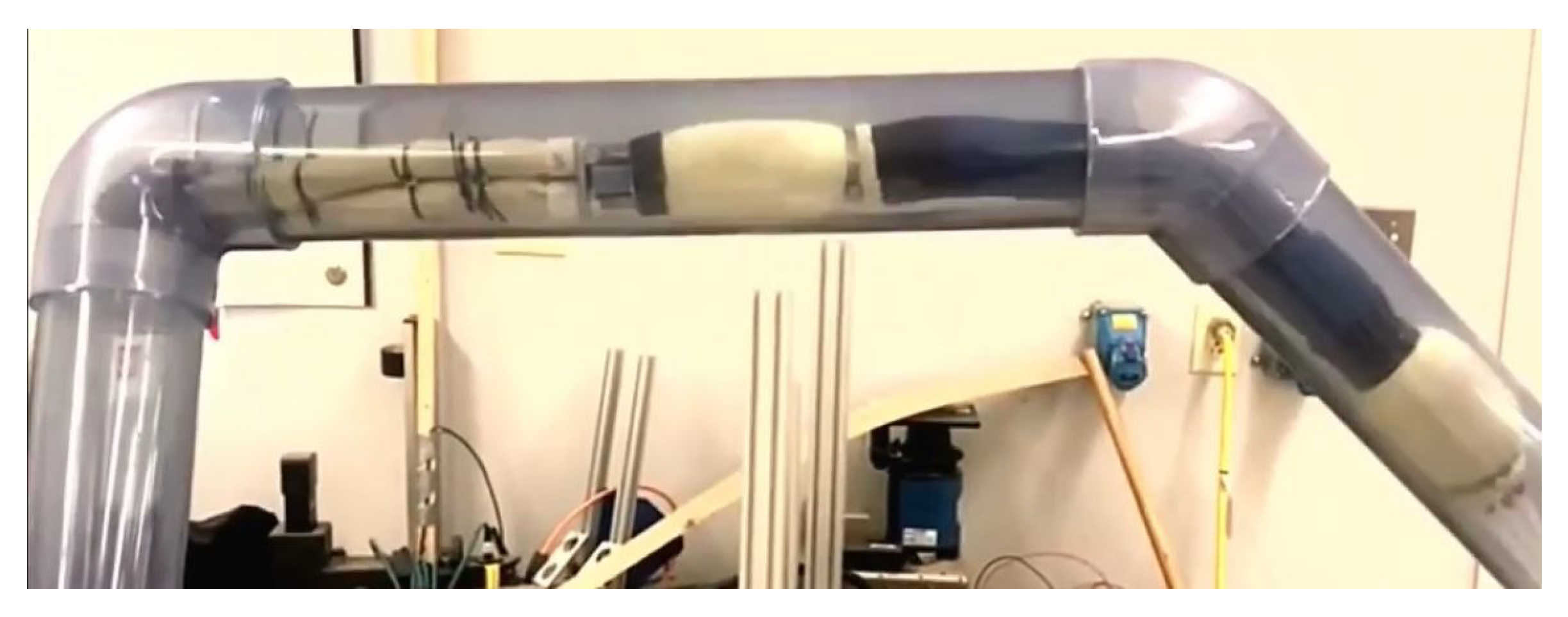
Additionally, an alternate version of the pipeworm was constructed by GE which used three PAMs and a triad of extensile PAMs manufactured by the Composites Research Laboratory at the University of Maryland, shown in Figure 19. The extensile PAMs use a low braid angle to allow the PAM to extend when inflated, allowing the triad to bend around corners [26]. This robot was capable of traveling through pipes at a speed of about 0.42 mm/s.

9. Conclusions

Analysis for the radial expansion force produced by a PAM is outlined in this study. This force, although utilized in robotic applications, has not been fully understood or properly modeled before, but understanding of the mechanics producing the force is necessary to ensure sufficient anchoring to support both the robot and any additional payload. The model not only accurately fit the data obtained from experimental testing both with and without applied axial loading but also aligned nicely with the axial contraction model, both in prediction of anchoring pressure and in calculated axial and circumferential bladder stress at the contact pressure.

Future work for this model includes performing slip tests of the PAM anchored in the pipe. These tests would entail anchoring the PAM in a pipe and increasing the axial load on the PAM until slip occurs. These tests would provide insight on how both friction and applied axial load affect slip to achieve a better understanding of how much payload a worm-like robot can carry before slipping occurs. Additional future work entails determining the cause for the misalignment of bladder stress between the axial contraction and radial expansion models, as well as the difference in moduli between the 76.2 mm (3 inch) and 88.9 mm (3.5 inch) data sets. Determining and resolving the cause could allow for a radial expansion model with moduli that work for any given pipe diameter, as opposed to needing a set of moduli for each pipe diameter of interest, as is currently the case.

The ability to accurately predict the anchoring force generated by PAMs allows for the possibility to accurately assess the needed level of pressurization to maintain anchoring in robotic applications where factors like pipe diameter or applied payload may vary along the course of the mission, allowing for a much broader scope and application of these types of robots.