Global Fixed-Time Fault-Tolerant Control for Tracked Vehicles with Hierarchical Unknown Input Observers

Abstract

This paper addresses the issues of sensor failures and actuator faults in mining tracked mobile vehicles (TMVs) operating in harsh environments by proposing a global fixed-time fault-tolerant control strategy based on a hierarchical unknown input observer structure. First, a kinematic and dynamic model of the TMV is established considering side slip and track slip, and its linear parameter-varying (LPV) model is constructed through parameter-dependent linearization. Then, a distributed structure consisting of four collaborating low-dimensional observers is designed, including a state observer, a disturbance observer, a position sensor fault observer, and a wheel speed sensor fault observer, and the fixed-time convergence of the closed-loop system is proven. Additionally, by equivalently treating actuator faults as power losses, an observer capable of identifying and compensating for motor efficiency losses is designed. Finally, an adaptive fault-tolerant control law is proposed by combining nominal control, disturbance compensation, and sliding mode switching terms, achieving global fixed-time stability and fault tolerance. Experimental results demonstrate that the proposed control system maintains excellent trajectory tracking performance even in the presence of sensor faults and actuator power losses, with tracking errors less than 0.1 m.

1. Introduction

Tracked mobile vehicles (TMV) exhibit superior traction, mobility, and traversability compared to wheeled vehicles, making them extensively applicable in industrial [1,2], agricultural [3], mining [4,5], and specialized domains. A typical application involves tracked auxiliary transport vehicles in coal mining operations, which can follow construction personnel to transport small equipment during tunnel excavation, significantly reducing the workload of construction workers and effectively improving excavation efficiency [6]. In such scenarios, TMVs typically follow the tunneling machine ahead, continuously transporting materials back and forth. Their operational trajectories are planned by construction personnel, enabling autonomous movement and following workers based on vision and radar systems mounted on the vehicles [7]. However, mining TMVs face multiple technical challenges in complex electromagnetic environments, including frequent sensor failures, actuator performance degradation, and complex contact dynamics between the tracks and ground. The coupling effects of these problems make precise trajectory tracking control exceptionally difficult, and traditional control methods often cannot guarantee system reliability and safety under fault conditions.

TMVs obtain pre-planned paths through vision and radar systems and perform real-time trajectory tracking control [8]. The tracked drive system relies on differential steering, and due to the driving characteristics of tracks, vehicles can only move in the direction of their body orientation, representing a typical nonholonomic constraint system [9]. Trajectory tracking control for nonholonomic constraint systems is highly complex, requiring consideration not only of system kinematics, dynamics, and coupling system effects, but also external disturbances caused by track slippage during steering, contact models between tracks and ground, and system uncertainties, making precise trajectory tracking control difficult to achieve [10,11]. More critically, existing methods face four core technical challenges: high-dimensional coupling observation problems caused by fault-tolerant system dimension augmentation, time uncertainty problems arising from traditional TMV operation control’s dependence on initial conditions without deterministic time-convergence guarantees, multi-source heterogeneous fault coupling problems caused by mutual influence between sensor and actuator failures, and precise control problems under nonholonomic constraints where control input dimensions are lower than state space dimensions. The existence of these challenges makes traditional control strategies perform poorly in practical applications.

Based on the above problems, numerous studies have recently explored dynamic control of TMVs. Similar to general Ackermann steering vehicles under nonholonomic constraints, TMV tracking control is mainly divided into two categories. One category is kinematic-based control, which generally treats the effects of vehicle dynamics as external disturbances. For instance, Refs. [12,13,14,15] all adopt similar schemes, compensating kinematic models based on slip observation and designing dynamic controllers for TMV tracking control. Another approach establishes coupled systems of kinematics and dynamics, with a general process of establishing kinematic and dynamic system models, building coupled models through Euler–Lagrange methods [11,16,17,18], and then designing nonlinear controllers based on these models, such as sliding mode control, adaptive control, model predictive control, and fuzzy control. However, these existing methods share common deficiencies: kinematic-based methods are computationally simple but have limited accuracy, with performance degrading rapidly under highly dynamic conditions; dynamics-coupled methods have higher accuracy but greater model complexity and strict parameter accuracy requirements, and all lack a systematic fault-tolerant design, meaning they are unable to handle simultaneous sensor and actuator failures.

TMV tracking control relies on state feedback, with typically deployed sensors including GNSS for pose acquisition and wheel speed sensors for capturing drive wheel rotational speed [19]. Some high-speed TMVs also install velocity sensors to enhance measurement accuracy and improve controller performance [20]. However, once sensors fail, controllers cannot guarantee original control accuracy, and systems may even completely lose stability [21]. Due to the complex electromagnetic environment of mining TMVs, even when sensors work normally, the effects of external signal interference cannot be ignored. Fault-tolerant controllers can maintain the system’s original performance when some sensors fail, and can even work when all sensors fail if the faults are modelable, showing significant application potential for the trajectory control of mobile equipment in interference environments and generating some research interest. Ref. [22] designed an adaptive sliding mode controller based on radial basis function neural networks, claiming to achieve the finite-time convergence of tracking errors even when ship propellers fail; Ref. [23] established an LPV model of vehicles, providing vehicle fault information through filters; Ref. [24] proposed a grouped sliding mode control method for hub motor failure problems in four-wheel independent drive vehicles; Ref. [25] constructed vehicle actuator fault buffers based on machine learning methods; Ref. [26] proposed a boundary function for ship constraint processing and developed a constraint-based trajectory controller; Ref. [27] used data fusion algorithms to detect and isolate sensor fault signals during vehicle autonomous driving. Although these studies achieved results under specific fault modes, three key limitations remain: first, existing methods mainly focus on single-fault modes, lacking multi-fault collaborative processing capabilities; second, most methods can only guarantee asymptotic convergence or finite-time convergence, with convergence time depending on initial conditions, and are therefore unable to provide deterministic time guarantees for safety-critical applications; third, observer design complexity is high, with traditional centralized observers facing dimensionality problems and difficulties guaranteeing real-time performance.

For mining TMVs, the challenge of fault-tolerant control schemes lies in the strict convergence time requirements. TMVs following construction personnel need to perform obstacle avoidance, and traditional controllers can only guarantee the asymptotic convergence of tracking errors, which makes it difficult to meet practical engineering requirements. Therefore, when external unknown signal inputs and actuator failures exist, achieving rapid convergence while maintaining system performance brings great challenges to TMV trajectory tracking controller design. More critically, sensor failures and actuator performance degradation in mining environments often occur simultaneously and are mutually coupled. Existing single-fault processing methods cannot handle such complex fault modes; therefore, a systematic fault-tolerant control method that can simultaneously handle multi-source heterogeneous faults, guarantee a deterministic convergence time, and reduce computational complexity is urgently required.

Based on the above analysis, this paper addresses the problems of sensor failures and actuator efficiency degradation faced by mining TMVs operating in complex electromagnetic environments by constructing a fault-tolerant controller system capable of achieving global fixed-time convergence. The proposed system establishes a parameter-dependent LPV model that considers lateral slip and track slippage, designs a distributed unknown input observer architecture comprising a state observer, a disturbance observer, a position sensor fault observer, and a wheel speed sensor fault observer, and incorporates an actuator efficiency observer. By employing an adaptive fault-tolerant control law based on bi-power sliding mode surface theory that integrates nominal control, disturbance compensation, and sliding mode switching terms, the system achieves precise trajectory tracking of tracked vehicles under conditions of sensor failures and actuator performance degradation.

The innovative contributions of this paper are twofold:

(1) A hierarchical collaborative observer architecture is proposed to address the fault observation problem of sensors and actuators, which decomposes the 17-dimensional high-dimensional observation problem into four low-dimensional sub-problems and ensures coupling stability through small gain conditions, thereby realizing the collaborative processing of multiple fault modes.

(2) The bi-power sliding mode surface theory is extended to TMV multi-fault coupling systems, establishing a fixed-time stability theory with convergence time upper bounds that are completely independent of initial conditions, and designing a globally fixed-time convergent fault-tolerant controller that provides deterministic time guarantees for safety-critical applications.

The structure of this paper is as follows: Section 1 introduces the research status and significance; Section 2 establishes the TMV model and LPV model; Section 3 presents the main design process of the grouped fault-tolerant observer; Section 4 provides the fault-tolerant controller design process; Section 5 validates the theoretical effectiveness through experiments; Section 6 presents the main conclusions of this paper.

2. Model Establishment

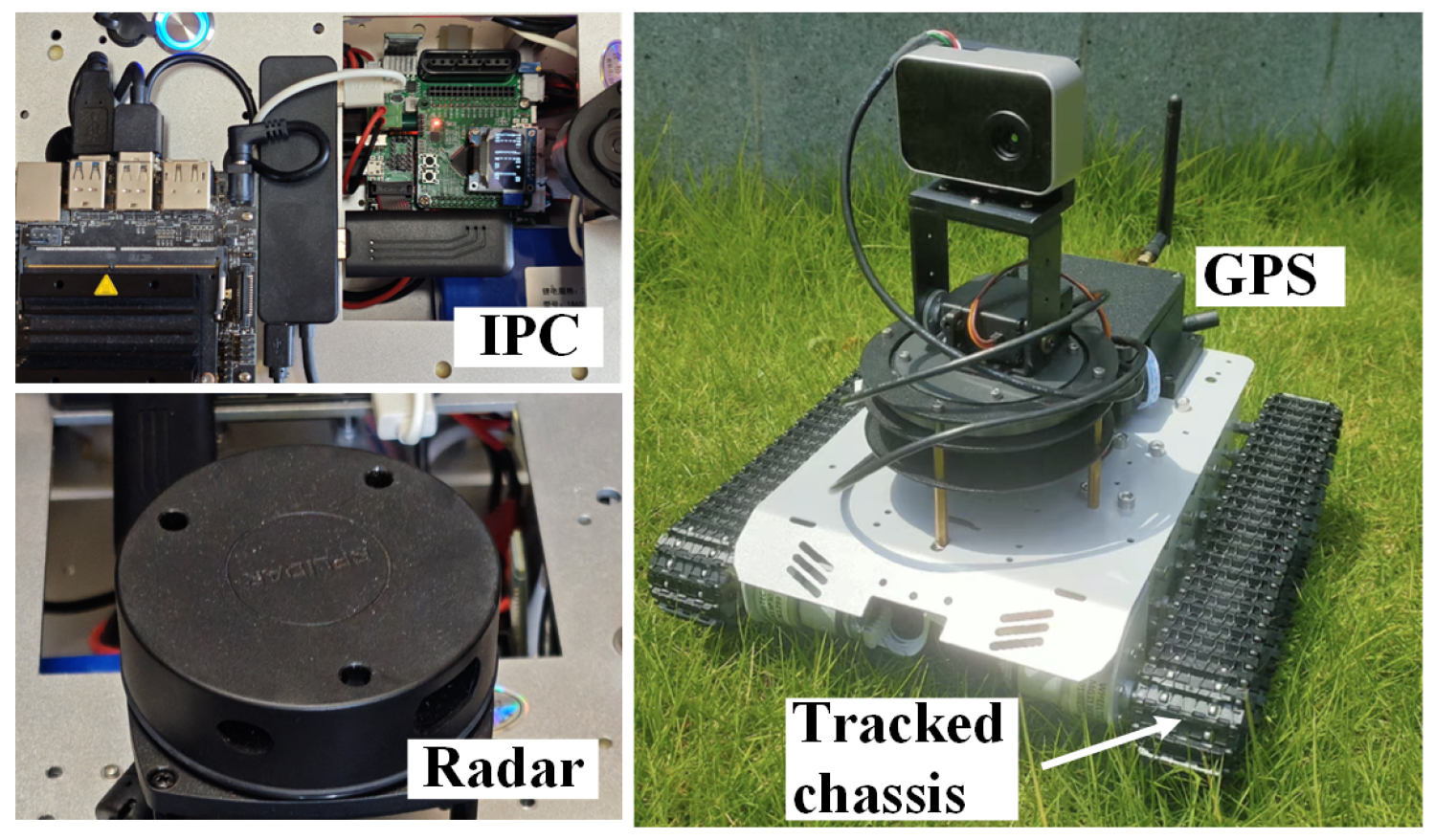
2.1. TMV System

The experimental TMV system is shown in Figure 1. This mobility platform consists of two parallel-mounted tracks, an industrial computer, GNSS, and vision and radar systems that are capable of traversing complex terrains. The platform integrates a Ublox ZED-F9P-01B high-precision GNSS module with RTK differential functionality, achieving ±2.5 cm horizontal positioning accuracy, meeting the high-precision requirements for posture data in experiments. The drive system monitoring employs Heidenhain ECN 413 series encoders, providing 2048 pulses per revolution with a resolution of 0.176°/pulse, making it capable of precisely capturing track motion characteristics and slip phenomena.

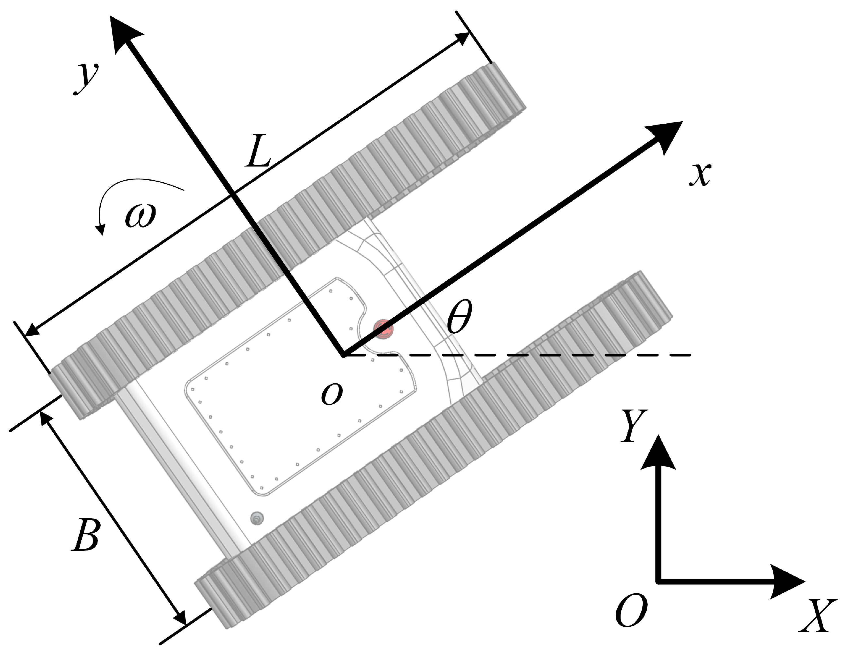
2.2. Kinematic Model

When establishing the TMV kinematic model, it is necessary to consider the actual motion characteristics of tracked vehicles. Unlike ideal rigid body motion, tracked vehicles exhibit complex sliding phenomena during turning processes. To accurately describe these phenomena while maintaining model tractability, this paper proposes the following reasonable assumptions based on the actual motion mechanism of tracked vehicles:

Assumption 1. 

Limited side slip is allowed during TMV turning, with the slip angle β defined as the angle between the vehicle’s longitudinal axis and the direction of velocity. When lateral sliding occurs, there exists lateral velocity in the vehicle coordinate system. Assume D is the offset distance of the vehicle’s running direction caused by track sliding during differential steering. The center of mass coincides with the geometric center of the vehicle.

The TMV movement direction is shown in Figure 2. The TMV wheel radius is r, the left and right wheel angular velocities are ${\mathrm{\Omega }}_L$ and ${\mathrm{\Omega }}_R$, and the slip rates are ${\mathrm{\Theta }}_L$ and ${\mathrm{\Theta }}_R$, respectively. When slippage occurs, the actual linear velocities of the left and right drive wheels are $v_L=r{\mathrm{\Omega }}_L(1-{\mathrm{\Theta }}_L)$, $v_R=r{\mathrm{\Omega }}_R(1-{\mathrm{\Theta }}_R)$. The slip rate $\mathrm{\Theta }$ represents the difference ratio between the actual linear velocity and the ideal linear velocity at the wheel–ground contact point—$\mathrm{\Theta }={\displaystyle \frac{r\mathrm{\Omega }-v}{r\mathrm{\Omega }}}$—where v is the actual linear velocity, and $r\mathrm{\Omega }$ is the ideal linear velocity. The velocity in the X direction in the TMV body coordinate system is as follows:

$$v_x={\displaystyle \frac{v_L+v_R}{2}}={\displaystyle \frac{r}{2}}\left[(1-{\mathrm{\Theta }}_L){\mathrm{\Omega }}_L+(1-{\mathrm{\Theta }}_R){\mathrm{\Omega }}_R\right]$$

(1)

The TMV rotational angular velocity is expressed as follows:

$$\omega ={\displaystyle \frac{v_R-v_L}{B}}={\displaystyle \frac{r}{B}}\left[(1-{\mathrm{\Theta }}_R){\mathrm{\Omega }}_R-(1-{\mathrm{\Theta }}_L){\mathrm{\Omega }}_L\right]$$

(2)

where B is the distance between the left and right wheels.

Considering side slip, the TMV’s lateral velocity consists of two components: one is the lateral component $-D\omega$ caused by the vehicle’s rotation, with the negative sign indicating an outward direction, and the other is the component $v_{x}tan\beta$ caused by side slip.

$$v_y=-D\omega +v_{x}tan\beta$$

(3)

where $D={\displaystyle \frac{L{a}_y}{2{\gamma }_{t}g}}cos\beta$ is the offset distance of the vehicle’s running direction caused by sliding, $a_y={\displaystyle \frac{v^2}{R^{\prime }}}sin\beta$ is the centripetal acceleration, and $R^{\prime }={\displaystyle \frac{\sqrt{v_x^2+v_y^2}}{\left|\omega \right|}}={\displaystyle \frac{B}{2cos\beta }}{\displaystyle \frac{{\mathrm{\Omega }}_L(1-{\mathrm{\Theta }}_L)+{\mathrm{\Omega }}_R(1-{\mathrm{\Theta }}_R)}{{\mathrm{\Omega }}_L(1-{\mathrm{\Theta }}_L)-{\mathrm{\Omega }}_R(1-{\mathrm{\Theta }}_R)}}$ is the instantaneous turning radius [18]; $\beta$ is the slip angle; L is the characteristic length of the track–ground contact; ${\gamma }_t$ is the friction coefficient between the track and the ground. The conversion between the body coordinate system and the global coordinate system is achieved through the rotation matrix:

$$\left[\begin{array}{c}\dot{X}\\ \dot{Y}\end{array}\right]=\left[\begin{array}{cc}cos\theta & -sin\theta \\ sin\theta & cos\theta \end{array}\right]\left[\begin{array}{c}{v}_x\\ v_y\end{array}\right]$$

(4)

The non-holonomic constraint equation for the TMV in the global coordinate system under Assumption 1 can be expressed as follows [4]:

$$-\dot{X}sin\theta +\dot{Y}cos\theta +D\omega =v_{x}tan\beta$$

(5)

Under non-holonomic constraints, the global motion equations of the TMV are as follows:

$$\left\{\begin{array}{c}\dot{X}=v_{x}cos\theta +D\omega sin\theta -v_{x}sin\theta tan\beta \hfill \\ \dot{Y}=v_{x}sin\theta -D\omega cos\theta +v_{x}cos\theta tan\beta \hfill \\ \dot{\theta }=\omega \hfill \end{array}\right.$$

(6)

2.3. Dynamic Model

The track driving force of the TMV is provided by motors, with torques output by the left and right motors being ${\tau }_L$ and ${\tau }_R$, respectively. The track driving force in the body coordinate system is expressed as follows:

$$F_{dx}={\displaystyle \frac{1}{2r}}({\tau }_L+{\tau }_R)$$

(7)

where r is the equivalent radius of the drive system. A body coordinate system is established with the center of mass as the origin, the x-axis along the longitudinal axis of the vehicle, and the y-axis perpendicular to the left. During TMV operation, the friction force is proportional to the normal force and opposite to the direction of motion:

$$\begin{array}{cc}\hfill F_{rLx}& =-{\displaystyle \frac{1}{2}}{\gamma }_{t}mg{\displaystyle \frac{v_x-\frac{B}{2}\omega }{|v_x-\frac{B}{2}\omega |+ϵ}},F_{rLy}=-{\displaystyle \frac{1}{2}}{\gamma }_{t}mg{\displaystyle \frac{v_y}{|v_x-\frac{B}{2}\omega |+ϵ}}\hfill \\ \hfill F_{rRx}& =-{\displaystyle \frac{1}{2}}{\gamma }_{t}mg{\displaystyle \frac{v_x+\frac{B}{2}\omega }{|v_x+\frac{B}{2}\omega |+ϵ}},F_{rRy}=-{\displaystyle \frac{1}{2}}{\gamma }_{t}mg{\displaystyle \frac{v_y}{|v_x+\frac{B}{2}\omega |+ϵ}}\hfill \end{array}$$

(8)

where B is the distance between the two tracks, and $ϵ$ is a very small positive number used to avoid division by zero. The total friction forces in the body coordinate system are $F_{rx}=F_{rLx}+F_{rRx}$, $F_{ry}=F_{rLy}+F_{rRy}$.

During TMV steering, the side slip force is proportional to the slip angle and acts along the y-axis of the vehicle body [28]:

$$F_l=2\mathrm{sgn}\left(\omega \right){\gamma }_{t}D{\displaystyle \frac{mg}{L}}$$

(9)

According to Newton’s second law and considering inertial forces in the rotating coordinate system, the dynamic equations of the TMV are as follows:

$$\left\{\begin{array}{c}M({\dot{v}}_x-v_y\omega )=F_{dx}-F_{rx}\hfill \\ M({\dot{v}}_y+v_x\omega )=-F_{ry}+F_l\hfill \\ I\dot{\omega }={\tau }_d-{\tau }_f-{\tau }_s\hfill \end{array}\right.$$

(10)

where M is the mass of the vehicle; I is the moment of inertia of the vehicle around the vertical axis; ${\tau }_d={\displaystyle \frac{r}{B}}({\tau }_R-{\tau }_L)$ is the driving torque; ${\tau }_f={\displaystyle \frac{B}{2}}(F_{rRx}-F_{rLx})$ is the friction torque; and ${\tau }_s=F_l·D=2\mathrm{sgn}\left(\omega \right){\gamma }_t{D}^2{\displaystyle \frac{mg}{L}}$ is the side slip torque.

Rearranging the above equations yields the following:

$$\left\{\begin{array}{c}{\dot{v}}_x={\displaystyle \frac{1}{M}}\left[{\displaystyle \frac{{\tau }_L+{\tau }_R}{2r}}-(F_{rRx}+F_{rLx})\right]+v_y\omega \hfill \\ {\dot{v}}_y={\displaystyle \frac{1}{M}}\left[2\mathrm{sgn}\left(\omega \right){\gamma }_{t}D{\displaystyle \frac{mg}{L}}-(F_{rRy}+F_{rLy})\right]-v_x\omega \hfill \\ \dot{\omega }={\displaystyle \frac{1}{I}}\left[{\displaystyle \frac{r({\tau }_R-{\tau }_L)}{B}}-{\displaystyle \frac{B}{2}}(F_{rRx}-F_{rLx})-2\mathrm{sgn}\left(\omega \right){\gamma }_t{D}^2{\displaystyle \frac{mg}{L}}\right]\hfill \end{array}\right.$$

(11)

2.4. LPV Model Establishment

Define the state variables and inputs as: $\mathbf{x}={\left[\begin{array}{cccccc}X& Y& \theta & v_x& v_y& \omega \end{array}\right]}^T$, $\mathbf{u}={\left[\begin{array}{cc}{\tau }_L& {\tau }_R\end{array}\right]}^T$. Define measurable scheduling parameters to represent the state-space equation: $\mathit{\rho }={\left[\begin{array}{cccc}cos\theta & sin\theta & v_x& \omega \end{array}\right]}^T$.

To simplify notation, let: ${\rho }_1=cos\theta$, ${\rho }_2=sin\theta$, ${\rho }_3=v_x$, ${\rho }_4=\omega$. Combining the aforementioned kinematic and dynamic models, the following LPV state-space expression can be constructed [29]:

$$\dot{\mathbf{x}}=\mathbf{A}\left(\mathit{\rho }\right)\mathbf{x}+\mathbf{B}\left(\mathit{\rho }\right)\mathbf{u}$$

(12)

where the system matrix $\mathbf{A}\left(\mathit{\rho }\right)$ and input matrix $\mathbf{B}\left(\mathit{\rho }\right)$ are as follows:

$$\mathbf{A}\left(\mathit{\rho }\right)=\left[\begin{array}{cccccc}0& 0& 0& a_{14}\left(\mathit{\rho }\right)& 0& a_{16}\left(\mathit{\rho }\right)\\ 0& 0& 0& a_{24}\left(\mathit{\rho }\right)& 0& a_{26}\left(\mathit{\rho }\right)\\ 0& 0& 0& 0& 0& 1\\ 0& 0& 0& a_{44}\left(\mathit{\rho }\right)& a_{45}\left(\mathit{\rho }\right)& a_{46}\left(\mathit{\rho }\right)\\ 0& 0& 0& a_{54}\left(\mathit{\rho }\right)& a_{55}\left(\mathit{\rho }\right)& a_{56}\left(\mathit{\rho }\right)\\ 0& 0& 0& a_{64}\left(\mathit{\rho }\right)& 0& a_{66}\left(\mathit{\rho }\right)\end{array}\right],$$

$$\mathbf{B}\left(\mathit{\rho }\right)=\left[\begin{array}{cc}0& 0\\ 0& 0\\ 0& 0\\ {\displaystyle \frac{1}{2Mr}}& {\displaystyle \frac{1}{2Mr}}\\ 0& 0\\ -{\displaystyle \frac{r}{BI}}& {\displaystyle \frac{r}{BI}}\end{array}\right]$$

(13)

where:

$$\begin{array}{cc}\hfill a_{14}\left(\mathit{\rho }\right)& ={\rho }_{1}cos\beta -{\rho }_{2}sin\beta \hfill \\ \hfill a_{16}\left(\mathit{\rho }\right)& =D{\rho }_2\hfill \\ \hfill a_{24}\left(\mathit{\rho }\right)& ={\rho }_{2}cos\beta +{\rho }_{1}sin\beta \hfill \\ \hfill a_{26}\left(\mathit{\rho }\right)& =-D{\rho }_1\hfill \\ \hfill a_{44}\left(\mathit{\rho }\right)& =-{\displaystyle \frac{1}{M}}(F_{rRx}^{\prime }+F_{rLx}^{\prime })\hfill \\ \hfill a_{45}\left(\mathit{\rho }\right)& ={\rho }_4\hfill \\ \hfill a_{46}\left(\mathit{\rho }\right)& =-{\displaystyle \frac{1}{M}}(F_{rRx}^{″}+F_{rLx}^{″})\hfill \\ \hfill a_{54}\left(\mathit{\rho }\right)& =-{\rho }_4\hfill \\ \hfill a_{55}\left(\mathit{\rho }\right)& =-{\displaystyle \frac{1}{M}}(F_{rRy}^{\prime }+F_{rLy}^{\prime })\hfill \\ \hfill a_{56}\left(\mathit{\rho }\right)& ={\displaystyle \frac{1}{M}}(2\mathrm{sgn}\left({\rho }_4\right){\gamma }_t{D}^{\prime }{\displaystyle \frac{mg}{L}}-(F_{rRy}^{″}+F_{rLy}^{″}))\hfill \\ \hfill a_{64}\left(\mathit{\rho }\right)& =-{\displaystyle \frac{B}{2I}}(F_{rRx}^{\prime }-F_{rLx}^{\prime })\hfill \\ \hfill a_{66}\left(\mathit{\rho }\right)& =-{\displaystyle \frac{1}{I}}({\displaystyle \frac{B}{2}}(F_{rRx}^{″}-F_{rLx}^{″})+2\mathrm{sgn}\left({\rho }_4\right){\gamma }_t{D}^{\prime 2}{\displaystyle \frac{mg}{L}})\hfill \end{array}$$

where $F_{(·)}^{\prime }$ and $F_{(·)}^{″}$ represent the partial derivatives of friction forces with respect to states $v_x$ and $\omega$, respectively; $D^{\prime }$ and $D^{\prime 2}$ represent the partial derivatives of D and $D^2$ with respect to $\omega$. The expanded expressions for these derivatives are as follows:

$$\begin{array}{cc}\hfill F_{rLx}^{\prime }& =-{\displaystyle \frac{1}{2}}{\gamma }_{t}mg{\displaystyle \frac{1}{|v_x-\frac{B}{2}\omega |+ϵ}}\times \left(1-{\displaystyle \frac{(v_x-\frac{B}{2}\omega )·\mathrm{sgn}(v_x-\frac{B}{2}\omega )}{|v_x-\frac{B}{2}\omega |+ϵ}}\right)\hfill \\ \hfill F_{rLx}^{″}& =-{\displaystyle \frac{1}{2}}{\gamma }_{t}mg{\displaystyle \frac{B}{2}}{\displaystyle \frac{1}{|v_x-\frac{B}{2}\omega |+ϵ}}\times \left(1+{\displaystyle \frac{(v_x-\frac{B}{2}\omega )·\mathrm{sgn}(v_x-\frac{B}{2}\omega )}{|v_x-\frac{B}{2}\omega |+ϵ}}\right)\hfill \end{array}$$

where the parameterized variables are as follows: slip angle $\beta$: $\beta =arctan\left({\displaystyle \frac{v_y}{{\rho }_3}}\right)$; offset distance D caused by sliding: $D={\displaystyle \frac{L{a}_y}{2{\gamma }_{t}g}}cos\beta$; and centripetal acceleration $a_y$: $a_y=\sqrt{v_x^2+v_y^2}·\omega sin\beta$.

3. Distributed Unknown Input Observer

3.1. System Construction

The LPV model of the TMV can be written as a system with external disturbances and sensor faults:

$$\left\{\begin{array}{c}\dot{\mathbf{x}}=\mathbf{A}\left(\mathit{\rho }\right)\mathbf{x}+\mathbf{B}\left(\mathit{\rho }\right)\mathbf{u}+\mathbf{d}\left(t\right)\hfill \\ \mathbf{y}=\mathbf{C}\mathbf{x}+\mathbf{F}\mathbf{f}\left(t\right)\hfill \end{array}\right.$$

(14)

where $\mathbf{d}\left(t\right)\in {\mathbb{R}}^6$ is the external disturbance vector, $\mathbf{f}\left(t\right)\in {\mathbb{R}}^5$ is the sensor fault vector, $\mathit{\rho }\left(t\right)\in {\mathbb{R}}^4$ is the time-varying scheduling parameter vector, and $\mathbf{F}\in {\mathbb{R}}^{5\times 5}$ is the full-rank sensor fault distribution matrix.

The system output measurements can be decomposed into position measurements and wheel speed measurement systems:

$$\mathbf{y}=\left[\begin{array}{c}{\mathbf{y}}_p{\mathbf{y}}_w\end{array}\right]=\left[\begin{array}{c}{\mathbf{C}}_p{\mathbf{C}}_w\end{array}\right]\mathbf{x}+\left[\begin{array}{ccc}{\mathbf{F}}_p& \mathbf{0}\mathbf{0}& {\mathbf{F}}_w\end{array}\right]\left[\begin{array}{c}{\mathbf{f}}_p{\mathbf{f}}_w\end{array}\right]$$

(15)

where ${\mathbf{y}}_p\in {\mathbb{R}}^3$ represents position-related measurements $(X,Y,\theta )$; ${\mathbf{y}}_w\in {\mathbb{R}}^2$ represents left and right wheel speed measurements $({\mathrm{\Omega }}_L,{\mathrm{\Omega }}_R)$; ${\mathbf{C}}_p\in {\mathbb{R}}^{3\times 6}$ is the position output matrix; ${\mathbf{C}}_w\in {\mathbb{R}}^{2\times 6}$ is the wheel speed output matrix; ${\mathbf{f}}_p\in {\mathbb{R}}^3$ is the position sensor fault vector; ${\mathbf{f}}_w\in {\mathbb{R}}^2$ is the wheel speed sensor fault vector; ${\mathbf{F}}_p\in {\mathbb{R}}^{3\times 3}$ and ${\mathbf{F}}_w\in {\mathbb{R}}^{2\times 2}$ are the corresponding fault distribution matrices; and the wheel speed output matrix is defined as follows:

$${\mathbf{C}}_w=\left[\begin{array}{cccccc}0& 0& 0& {\displaystyle \frac{1}{r}}& 0& -{\displaystyle \frac{B}{2r}}\\ 0& 0& 0& {\displaystyle \frac{1}{r}}& 0& {\displaystyle \frac{B}{2r}}\end{array}\right]$$

(16)

Assumption 2. 

In the subsequent design process, it is assumed that the following signals in the system are bounded and differentiable: the external disturbance $\mathbf{d}\left(t\right)$ and its derivative satisfy $\parallel \mathbf{d}\left(t\right)\parallel \le d_{max}$, $\parallel \dot{\mathbf{d}}\left(t\right)\parallel \le {\dot{d}}_{max}$; the sensor fault $\mathbf{f}\left(t\right)$ and its derivative satisfy $\parallel \mathbf{f}\left(t\right)\parallel \le f_{max}$, $\parallel \dot{\mathbf{f}}\left(t\right)\parallel \le {\dot{f}}_{max}$; the time-varying scheduling parameter $\mathit{\rho }\left(t\right)$ and its derivative satisfy $\parallel \mathit{\rho }\left(t\right)\parallel \le \overline{\mathit{\rho }}$, $\parallel \dot{\mathit{\rho }}\left(t\right)\parallel \le \overline{\nu }$; the actuator efficiency loss factor $\mathit{\eta }\left(t\right)$ changes slowly, satisfying $\parallel \dot{\mathit{\eta }}\left(t\right)\parallel \le {\mathrm{\Delta }}_{\eta }$; and the measurement noise $\mathit{\xi }\left(t\right)$ and its higher-order derivatives are bounded, satisfying $\parallel \mathit{\xi }\left(t\right)\parallel \le {\mathrm{\Delta }}_{\xi }$, $\parallel \ddot{\mathit{\xi }}\left(t\right)\parallel \le {\mathrm{\Delta }}_{\ddot{\xi }}$.

These requirements are reasonable in practical engineering applications for the following reasons:

1.

External disturbances such as friction forces and lateral slip forces between tracks and ground are physically bounded by nature, and their rates of change are constrained by the inertia of the mechanical system;

2.

Sensor faults typically manifest as gradual processes rather than abrupt changes, thereby ensuring that fault signals and their derivatives exhibit bounded characteristics;

3.

Time-varying scheduling parameters reflect the operational states of the system, and their variations remain smooth during continuous operation;

4.

Motor efficiency degradation represents a slow aging process that does not undergo sudden changes during normal operation;

5.

Measurement noise in practical applications generally satisfies statistical boundedness requirements.

To simultaneously estimate states, disturbances, and faults, the disturbance $\mathbf{d}\left(t\right)$ and fault $\mathbf{f}\left(t\right)$ are treated as augmented states, defining the augmented state vector:

$$\mathbf{z}={\left[\begin{array}{cccc}{\mathbf{x}}^T& {\mathbf{d}}^T& {\mathbf{f}}_p^T& {\mathbf{f}}_w^T\end{array}\right]}^T\in {\mathbb{R}}^{17}$$

(17)

The dynamics equation of the augmented system is as follows:

$$\begin{array}{cc}\hfill \dot{\mathbf{z}}& =\left[\begin{array}{c}\dot{\mathbf{x}}\\ \dot{\mathbf{d}}\\ {\dot{\mathbf{f}}}_p\\ {\dot{\mathbf{f}}}_w\end{array}\right]=\left[\begin{array}{c}\mathbf{A}\left(\mathit{\rho }\right)\mathbf{x}+\mathbf{B}\left(\mathit{\rho }\right)\mathbf{u}+\mathbf{d}\\ {\mathbf{w}}_d\left(t\right)\\ {\mathbf{w}}_{f_p}\left(t\right)\\ {\mathbf{w}}_{f_w}\left(t\right)\end{array}\right]\hfill \\ \hfill & =\left[\begin{array}{cccc}\mathbf{A}\left(\mathit{\rho }\right)& {\mathbf{I}}_6& {\mathbf{0}}_{6\times 3}& {\mathbf{0}}_{6\times 2}\\ {\mathbf{0}}_{6\times 6}& {\mathbf{0}}_{6\times 6}& {\mathbf{0}}_{6\times 3}& {\mathbf{0}}_{6\times 2}\\ {\mathbf{0}}_{3\times 6}& {\mathbf{0}}_{3\times 6}& {\mathbf{0}}_{3\times 3}& {\mathbf{0}}_{3\times 2}\\ {\mathbf{0}}_{2\times 6}& {\mathbf{0}}_{2\times 6}& {\mathbf{0}}_{2\times 3}& {\mathbf{0}}_{2\times 2}\end{array}\right]\mathbf{z}+\left[\begin{array}{c}\mathbf{B}\left(\mathit{\rho }\right)\\ {\mathbf{0}}_{6\times 2}\\ {\mathbf{0}}_{3\times 2}\\ {\mathbf{0}}_{2\times 2}\end{array}\right]\mathbf{u}+\left[\begin{array}{c}{\mathbf{0}}_n\\ {\mathbf{w}}_d\left(t\right)\\ {\mathbf{w}}_{f_p}\left(t\right)\\ {\mathbf{w}}_{f_w}\left(t\right)\end{array}\right]\hfill \\ \hfill & =\mathcal{A}\left(\mathit{\rho }\right)\mathbf{z}+\mathcal{B}\left(\mathit{\rho }\right)\mathbf{u}+\mathbf{w}\left(t\right)\hfill \end{array}$$

(18)

The system output equation can be expressed as follows:

$$\begin{array}{cc}\hfill \mathbf{y}& =\left[\begin{array}{c}{\mathbf{y}}_p\\ {\mathbf{y}}_w\end{array}\right]=\left[\begin{array}{cccc}{\mathbf{C}}_p& {\mathbf{0}}_{3\times 6}& {\mathbf{F}}_p& {\mathbf{0}}_{3\times 2}\\ {\mathbf{C}}_w& {\mathbf{0}}_{2\times 6}& {\mathbf{0}}_{2\times 3}& {\mathbf{F}}_w\end{array}\right]\mathbf{z}=\mathcal{C}\mathbf{z}\hfill \end{array}$$

(19)

The augmented system has a dimension of 17, and directly designing a NUIO for it would increase computational complexity, making it difficult to obtain accurate estimates of the system states, disturbances, and faults. In the following, a distributed structure of UNIO will be established, decomposing the high-dimensional observer into four low-dimensional observers that collaborate with each other: the state observer, which estimates position and velocity states $\widehat{\mathbf{x}}$; the disturbance observer, which estimates external disturbances $\widehat{\mathbf{d}}$; the position sensor fault observer, which estimates position and orientation angle sensor faults ${\widehat{\mathbf{f}}}_p$; and the wheel speed sensor fault observer, which estimates wheel speed sensor faults ${\widehat{\mathbf{f}}}_w$. The complete output equation can be rewritten as follows:

$$\mathbf{y}=\left[\begin{array}{c}{\mathbf{y}}_p\\ {\mathbf{y}}_w\end{array}\right]=\left[\begin{array}{c}{\mathbf{C}}_p\\ {\mathbf{C}}_w\end{array}\right]\mathbf{x}+\left[\begin{array}{cc}{\mathbf{F}}_p& \mathbf{0}\\ \mathbf{0}& {\mathbf{F}}_w\end{array}\right]\left[\begin{array}{c}{\mathbf{f}}_p\\ {\mathbf{f}}_w\end{array}\right]$$

(20)

The wheel speed sensor fault distribution matrix is as follows: ${\mathbf{F}}_p={\mathbf{I}}_{3\times 3},{\mathbf{F}}_w={\mathbf{I}}_{2\times 2}$, representing the independence of faults in the left and right wheel speed sensors.

The working principle of the distributed NUIO can be described as follow. When no fault occurs, the disturbance observer and sensor fault observer rely on measured states for estimation, during which the output values of the state observer are not used, reducing error propagation caused by state estimation; once a faulty sensor is detected, the reconstructed value of the sensor is used instead of the measured value, and the state observer compensates in real-time for the estimation results from the disturbance observer and the two types of fault observers through sliding mode feedback terms. The distributed structure not only reduces the computational complexity of high-dimensional systems but also achieves an optimal balance between state estimation, disturbance suppression, and fault detection.

3.2. Fixed-Time Differentiator

Lemma 1. 

Consider a system $\dot{\mathbf{x}}=\mathbf{f}(t,\mathbf{x})$. If there exists a continuously positive definite function $V\left(\mathbf{x}\right):{\mathbb{R}}^n\to {\mathbb{R}}_{+}$ satisfying

$$\dot{V}\left(\mathbf{x}\right)\le -k_1{V}^{\alpha }\left(\mathbf{x}\right)-k_2{V}^{\beta }\left(\mathbf{x}\right)$$

(21)

where $k_1,k_2>0$, $0<\alpha <1$, $\beta >1$, then the system is fixed-time stable around the equilibrium point, and the upper bound of the convergence time is [30]

$$T\le {\displaystyle \frac{1}{k_1(1-\alpha )}}+{\displaystyle \frac{1}{k_2(\beta -1)}}$$

(22)

and this upper bound is independent of the initial condition $\mathbf{x}\left(0\right)$.

Based on the fixed-time convergence principle (Lemma 1), the structure of a dual-power sliding mode surface is given as follows [31]:

$${\mathbf{s}}_x={\mathbf{e}}_x+{\gamma }_x{\int }_0^t\left(\parallel {\mathbf{e}}_x{\parallel }^{p_x}\mathrm{sign}\left({\mathbf{e}}_x\right)+{\parallel {\mathbf{e}}_x\parallel }^{q_x}\mathrm{sign}\left({\mathbf{e}}_x\right)\right)d\tau$$

(23)

where:${\mathbf{e}}_x=\mathbf{x}-\widehat{\mathbf{x}}$ is the state estimation error; ${\gamma }_x>0$ is a design parameter; and $p_x\in (0,1)$ and $q_x>1$ are power parameters. The term $\parallel {\mathbf{e}}_x{\parallel }^{p_x}\mathrm{sign}\left({\mathbf{e}}_x\right)$ plays a dominant role when the error is large, accelerating convergence away from the equilibrium point; and the term $\parallel {\mathbf{e}}_x{\parallel }^{q_x}\mathrm{sign}\left({\mathbf{e}}_x\right)$ plays a dominant role when the error is small, accelerating convergence approaching the equilibrium point.

In the subsequent design, the second-order derivatives of the TMV pose, i.e., acceleration, are needed, but actual measurements and observations can only obtain velocity values. The direct differentiation of velocity values would lead to noise amplification. To avoid using acceleration terms, inspired by command filtering control techniques, a Levant differentiator [32] with dual-power sliding mode terms is introduced as a command filter to achieve fixed-time convergence. The differentiator design for $v_x$ is as follows:

$$\left\{\begin{array}{c}{\dot{\phi }}_1=\psi \hfill \\ \psi =-k_1^L{|{\phi }_1-v_x^{\mathrm{m}}|}^{p_L}\mathrm{sign}({\phi }_1-v_x^{\mathrm{m}})\hfill \\ -k_2^L{|{\phi }_1-v_x^{\mathrm{m}}|}^{q_L}\mathrm{sign}({\phi }_1-v_x^{\mathrm{m}})+{\phi }_2\hfill \\ {\dot{\phi }}_2=-k_3^L\mathrm{sign}({\phi }_2-\psi )\hfill \end{array}\right.$$

(24)

where local ${\phi }_1$ is the velocity estimate; ${\phi }_2$ is the local acceleration estimate; and $k_1^L,k_2^L,k_3^L>0$ are design parameters, $0<p_L<1$, $q_L>1$. The output estimates are ${\widehat{v}}_x={\phi }_1$, ${\widehat{\dot{v}}}_x={\phi }_2$.

Theorem 1. 

Consider the improved Levant differentiator system (1), assuming that the second-order derivative of the measurement noise ξ is bounded, i.e., $|\ddot{\xi }|\le {\mathrm{\Delta }}_{\ddot{\xi }}$. If the parameters are selected to satisfy $p_L=0.5$, $q_L=1.5$, $k_2^L=1.1k_1^L$ and $k_3^L>1.5\sqrt{k_1^L}+L_L$, where $L_L\ge \left|{\ddot{v}}_x\right|+{\mathrm{\Delta }}_{\ddot{\xi }}$, then the system will converge in fixed time from any initial condition to a tight set related to the amplitude of higher-order derivatives of the noise, with an upper bound on the convergence time of

$$\begin{array}{c}\hfill T_L\le {\displaystyle \frac{3}{k_1^{\prime }}}+{\displaystyle \frac{2}{k_2^{\prime }}}\end{array}$$

(25)

where $k_1^{\prime }$ and $k_2^{\prime }$ are positive constants depending on the system parameters.

Proof. 

Define the velocity differentiation estimation errors as follows: $e_1={\phi }_1-v_x$, $e_2={\phi }_2-{\dot{v}}_x$. Considering the measurement noise $\xi =v_x^{\mathrm{m}}-v_x$, we have $v_x^{\mathrm{m}}=v_x+\xi$. Define an auxiliary variable ${\sigma }_L={\phi }_1-v_x^{\mathrm{m}}=e_1-\xi$. The time derivative of $\sigma$ is as follows: $-k_1^L{\left|\sigma \right|}^{p_L}\mathrm{sign}\left(\sigma \right)-k_2^L{\left|\sigma \right|}^{q_L}\mathrm{sign}\left(\sigma \right)+e_2-\dot{\xi }$.

The time derivatives of the differentiation estimation errors are as follows:

$$\begin{array}{cc}\hfill {\dot{e}}_1& ={\dot{\phi }}_1-{\dot{v}}_x\hfill \\ \hfill & =\psi -{\dot{v}}_x\hfill \\ \hfill & =-k_1^L{\left|\sigma \right|}^{p_L}\mathrm{sign}\left(\sigma \right)-k_2^L{\left|\sigma \right|}^{q_L}\mathrm{sign}\left(\sigma \right)+{\phi }_2-{\dot{v}}_x\hfill \\ \hfill & =-k_1^L{\left|\sigma \right|}^{p_L}\mathrm{sign}\left(\sigma \right)-k_2^L{\left|\sigma \right|}^{q_L}\mathrm{sign}\left(\sigma \right)+e_2+{\dot{v}}_x-{\dot{v}}_x\hfill \\ \hfill & =-k_1^L{\left|\sigma \right|}^{p_L}\mathrm{sign}\left(\sigma \right)-k_2^L{\left|\sigma \right|}^{q_L}\mathrm{sign}\left(\sigma \right)+e_2\hfill \\ \hfill {\dot{e}}_2& ={\dot{\phi }}_2-{\ddot{v}}_x\hfill \\ \hfill & =-k_3^L\mathrm{sign}({\phi }_2-\psi )-{\ddot{v}}_x\hfill \end{array}$$

(26)

Construct a Lyapunov function for the differentiation estimation error:

$$V_L=c_1^L{\left|\sigma \right|}^{1+p_L}+c_2^L{\left|\sigma \right|}^{1-p_L}|e_2{|}^2+c_3^L\left|e_2\right|$$

(27)

where $c_1^L$, $c_2^L$, $c_3^L$ are positive constants to be determined. The time derivative of $V_L$ is as follows:

$$\begin{array}{cc}\hfill {\dot{V}}_L& =c_1^L(1+p_L){\left|\sigma \right|}^{p_L}\mathrm{sign}\left(\sigma \right)·\dot{\sigma }\hfill \\ \hfill & +c_2^L(1-p_L){\left|\sigma \right|}^{-p_L}\mathrm{sign}\left(\sigma \right)·\dot{\sigma }·{\left|e_2\right|}^2\hfill \\ \hfill & +c_2^L{\left|\sigma \right|}^{1-p_L}·2\left|e_2\right|·\mathrm{sign}\left(e_2\right)·{\dot{e}}_2\hfill \\ \hfill & +c_3^L\mathrm{sign}\left(e_2\right)·{\dot{e}}_2\hfill \end{array}$$

(28)

Substituting $\dot{\sigma }$ and ${\dot{e}}_2$:

$$\begin{array}{cc}\hfill {\dot{V}}_L& =c_1^L(1+p_L){\left|\sigma \right|}^{p_L}\mathrm{sign}\left(\sigma \right)·(-k_1^L{\left|\sigma \right|}^{p_L}\mathrm{sign}\left(\sigma \right)\hfill \\ \hfill & -k_2^L{\left|\sigma \right|}^{q_L}\mathrm{sign}\left(\sigma \right)+e_2-\dot{\xi })\hfill \\ \hfill & +c_2^L(1-p_L){\left|\sigma \right|}^{-p_L}\mathrm{sign}\left(\sigma \right)·(-k_1^L{\left|\sigma \right|}^{p_L}\mathrm{sign}\left(\sigma \right)\hfill \\ \hfill & -k_2^L{\left|\sigma \right|}^{q_L}\mathrm{sign}\left(\sigma \right)+e_2-\dot{\xi })·{\left|e_2\right|}^2\hfill \\ \hfill & +c_2^L{\left|\sigma \right|}^{1-p_L}·2\left|e_2\right|·\mathrm{sign}\left(e_2\right)·(-k_3^L\mathrm{sign}\left(\sigma \right)-{\ddot{v}}_x)\hfill \\ \hfill & +c_3^L\mathrm{sign}\left(e_2\right)·(-k_3^L\mathrm{sign}\left(\sigma \right)-{\ddot{v}}_x)\hfill \end{array}$$

(29)

Expanding and reorganizing:

$$\begin{array}{cc}\hfill {\dot{V}}_L& =-c_1^L(1+p_L)k_1^L{\left|\sigma \right|}^{2p_L}-c_1^L(1+p_L)k_2^L{\left|\sigma \right|}^{p_L+q_L}\hfill \\ \hfill & +c_1^L(1+p_L){\left|\sigma \right|}^{p_L}\mathrm{sign}\left(\sigma \right)·e_2\hfill \\ \hfill & -c_1^L(1+p_L){\left|\sigma \right|}^{p_L}\mathrm{sign}\left(\sigma \right)·\dot{\xi }\hfill \\ \hfill & -c_2^L(1-p_L)k_1^L|e_2{|}^2-c_2^L(1-p_L)k_2^L{\left|\sigma \right|}^{q_L-p_L}{\left|e_2\right|}^2\hfill \\ \hfill & +c_2^L(1-p_L){\left|\sigma \right|}^{-p_L}\mathrm{sign}\left(\sigma \right)·e_2·{\left|e_2\right|}^2\hfill \\ \hfill & -c_2^L(1-p_L){\left|\sigma \right|}^{-p_L}\mathrm{sign}\left(\sigma \right)·\dot{\xi }·{\left|e_2\right|}^2\hfill \\ \hfill & -c_2^L{\left|\sigma \right|}^{1-p_L}·2\left|e_2\right|·\mathrm{sign}\left(e_2\right)·k_3^L\mathrm{sign}\left(\sigma \right)\hfill \\ \hfill & -c_2^L{\left|\sigma \right|}^{1-p_L}·2\left|e_2\right|·\mathrm{sign}\left(e_2\right)·{\ddot{v}}_x\hfill \\ \hfill & -c_3^L\mathrm{sign}\left(e_2\right)·k_3^L\mathrm{sign}\left(\sigma \right)-c_3^L\mathrm{sign}\left(e_2\right)·{\ddot{v}}_x\hfill \end{array}$$

(30)

Using Young’s inequality, and letting: $c_1^L={\displaystyle \frac{1}{(1+p_L)k_1^L}}$, $c_2^L={\displaystyle \frac{1}{(1-p_L)k_1^L}}$, $c_3^L={\displaystyle \frac{2k_3^L}{L+k_3^L}}$, using the equivalence relationship between $V_L$ and the state variables, such that there exist positive constants $k_1^{\prime }$ and $k_2^{\prime }$ and a bounded disturbance term $\gamma$, making

$$\begin{array}{cc}\hfill {\dot{V}}_L& \le -c_1^L(1+p_L)k_1^L{\left|\sigma \right|}^{2p_L}-c_1^L(1+p_L)k_2^L{\left|\sigma \right|}^{p_L+q_L}\hfill \\ \hfill & +c_1^L(1+p_L){\left|\sigma \right|}^{p_L}\mathrm{sign}\left(\sigma \right)·e_2\hfill \\ \hfill & +{\displaystyle \frac{1}{2}}{c}_1^L(1+p_L)k_1^L{\left|\sigma \right|}^{2p_L}+{\displaystyle \frac{c_1^L(1+p_L){\left|\dot{\xi }\right|}^2}{2k_1^L}}\hfill \\ \hfill & -c_2^L(1-p_L)k_1^L|e_2{|}^2-c_2^L(1-p_L)k_2^L{\left|\sigma \right|}^{q_L-p_L}{\left|e_2\right|}^2\hfill \\ \hfill & +c_2^L(1-p_L){\left|\sigma \right|}^{-p_L}\mathrm{sign}\left(\sigma \right)·e_2·{\left|e_2\right|}^2\hfill \\ \hfill & -c_2^L(1-p_L){\left|\sigma \right|}^{-p_L}\mathrm{sign}\left(\sigma \right)·\dot{\xi }·{\left|e_2\right|}^2\hfill \\ \hfill & +c_2^L{\left|\sigma \right|}^{1-p_L}·2|e_2|·k_3^L-c_2^L{\left|\sigma \right|}^{1-p_L}·2\left|e_2\right|·L_v\hfill \\ \hfill & +c_3^L{k}_3^L+c_3^L{L}_v\hfill \\ \hfill & \le -k_1^{\prime }{V}_L^{2/3}-k_2^{\prime }{V}_L^{3/2}+{\gamma }_{\xi }\hfill \end{array}$$

(31)

where ${\gamma }_{\xi }$ is a bounded constant related to the amplitude of higher-order derivatives of the noise, ${\gamma }_{\xi }=\mathcal{O}({\mathrm{\Delta }}_{\dot{\xi }}^2+{\mathrm{\Delta }}_{\ddot{\xi }})$. According to Lemma 1, in the absence of disturbance (i.e., ${\gamma }_{\xi }=0$), the upper bound of the system convergence time is as follows:

$$T_L\le {\displaystyle \frac{1}{k_1^{\prime }(1-2/3)}}+{\displaystyle \frac{1}{k_2^{\prime }(3/2-1)}}={\displaystyle \frac{3}{k_1^{\prime }}}+{\displaystyle \frac{2}{k_2^{\prime }}}$$

(32)

When disturbances exist, the system converges in fixed time to a tight set related to ${\gamma }_{\xi }$: ${lim}_{t\to T_L}{V}_L\left(t\right)\le \mathrm{\Omega }\left({\gamma }_{\xi }\right)$, where $\mathrm{\Omega }\left({\gamma }_{\xi }\right)$ represents a bounded value positively correlated with ${\gamma }_{\xi }$. The design process for the differentiators of $v_y$ and $\omega$ is similar to the above, and their design and proof processes will not be elaborated further. □

3.3. State Observer

Assumption 3. 

The fixed-time differentiator (24) designed above converges within time $T_L$, with its acceleration estimation error satisfying $\parallel {\mathrm{\Delta }}_{\ddot{\mathbf{v}}}\parallel \le {\mathrm{\Delta }}_{max}$, and ${\mathrm{\Delta }}_{max}\le {\displaystyle \frac{d_{max}}{K_{\mathit{absorb}}}}$, where $K_{\mathit{absorb}}\ge 1$ is a design constant.

The dynamics equation of the state observer is designed as follows:

$$\begin{array}{cc}\hfill \dot{\widehat{\mathbf{x}}}& =\mathbf{A}\left(\mathit{\rho }\right)\widehat{\mathbf{x}}+\mathbf{B}\left(\mathit{\rho }\right)\mathbf{u}+{\mathbf{L}}_x\left(\mathit{\rho }\right)(\mathbf{y}-\mathbf{C}\widehat{\mathbf{x}}-\mathbf{F}\widehat{\mathbf{f}})+{\mathbf{v}}_x\hfill \end{array}$$

(33)

where ${\mathbf{L}}_x\left(\mathit{\rho }\right)$ is the parameter-dependent linear feedback gain; ${\mathbf{v}}_x=-{\mu }_{x1}\parallel {\mathbf{s}}_x{\parallel }^{p_x-1}{\mathbf{s}}_x-{\mu }_{x2}{\parallel {\mathbf{s}}_x\parallel }^{q_x-1}{\mathbf{s}}_x$ is the sliding mode term; ${\mu }_{x1},{\mu }_{x2}>0$, $({\mathbf{s}}_x\ne 0)$ are sliding mode term gains; $p_x,q_x$ are sliding mode term power parameters; and $\widehat{\mathbf{f}}={[{\widehat{\mathbf{f}}}_p^T,{\widehat{\mathbf{f}}}_w^T]}^T$ is the combined fault estimation vector. If defining the system state estimation error as ${\mathbf{e}}_x=\mathbf{x}-\widehat{\mathbf{x}}$, taking the time derivative yields the following:

$$\begin{array}{cc}\hfill {\dot{\mathbf{e}}}_x& =\dot{\mathbf{x}}-\dot{\widehat{\mathbf{x}}}\hfill \\ \hfill & =\mathbf{A}\left(\mathit{\rho }\right)\mathbf{x}+\mathbf{B}\left(\mathit{\rho }\right)\mathbf{u}+\mathbf{d}-\mathbf{A}\left(\mathit{\rho }\right)\widehat{\mathbf{x}}-\mathbf{B}\left(\mathit{\rho }\right)\mathbf{u}\hfill \\ \hfill & -{\mathbf{L}}_x\left(\mathit{\rho }\right)(\mathbf{y}-\mathbf{C}\widehat{\mathbf{x}}-\mathbf{F}\widehat{\mathbf{f}})+{\mathbf{v}}_x\hfill \\ \hfill & =\mathbf{A}\left(\mathit{\rho }\right)\mathbf{x}+\mathbf{B}\left(\mathit{\rho }\right)\mathbf{u}+\mathbf{d}-\mathbf{A}\left(\mathit{\rho }\right)\widehat{\mathbf{x}}-\mathbf{B}\left(\mathit{\rho }\right)\mathbf{u}\hfill \\ \hfill & -{\mathbf{L}}_x\left(\mathit{\rho }\right)(\mathbf{C}\mathbf{x}+\mathbf{F}\mathbf{f}-\mathbf{C}\widehat{\mathbf{x}}-\mathbf{F}\widehat{\mathbf{f}})+{\mathbf{v}}_x\hfill \\ \hfill & =\mathbf{A}\left(\mathit{\rho }\right)(\mathbf{x}-\widehat{\mathbf{x}})+\mathbf{d}-{\mathbf{L}}_x\left(\mathit{\rho }\right)\mathbf{C}(\mathbf{x}-\widehat{\mathbf{x}})\hfill \\ \hfill & -{\mathbf{L}}_x\left(\mathit{\rho }\right)\mathbf{F}(\mathbf{f}-\widehat{\mathbf{f}})+{\mathbf{v}}_x\hfill \\ \hfill & =\mathbf{A}\left(\mathit{\rho }\right)(\mathbf{x}-\widehat{\mathbf{x}})+\mathbf{d}-{\mathbf{L}}_x\left(\mathit{\rho }\right)\mathbf{C}(\mathbf{x}-\widehat{\mathbf{x}})\hfill \\ \hfill & -{\mathbf{L}}_x\left(\mathit{\rho }\right)\mathbf{F}(\mathbf{f}-\widehat{\mathbf{f}})+{\mathbf{v}}_x\hfill \end{array}$$

(34)

Based on the parameter-dependent Lyapunov method, the linear feedback gain matrix ${\mathbf{L}}_x\left(\mathit{\rho }\right)$ is expressed as follows:

$${\mathbf{L}}_x\left(\mathit{\rho }\right)={\mathbf{P}}_x^{-1}\left(\mathit{\rho }\right){\mathbf{C}}^T{\mathbf{W}}_x\left(\mathit{\rho }\right)$$

(35)

where ${\mathbf{P}}_x\left(\mathit{\rho }\right)$ is a parameter-dependent positive definite matrix satisfying the following linear matrix inequality (LMI):

$$2{\mathbf{P}}_x\left(\mathit{\rho }\right)\mathbf{A}\left(\mathit{\rho }\right)-2{\mathbf{C}}^T{\mathbf{W}}_x\left(\mathit{\rho }\right)\mathbf{C}+{\dot{\mathbf{P}}}_x\left(\mathit{\rho }\right)+{\mathbf{Q}}_x\left(\mathit{\rho }\right)⪯0$$

(36)

where ${\mathbf{Q}}_x\left(\mathit{\rho }\right)\succ 0$ is a design parameter matrix.

To prove the stability of the state observer, select the Lyapunov function $V_x={\displaystyle \frac{1}{2}}{\mathbf{s}}_x^T{\mathbf{P}}_x{\mathbf{s}}_x$, where ${\mathbf{P}}_x$ is a symmetric positive definite matrix. The time derivative of the Lyapunov function is as follows:

$$\begin{array}{cc}\hfill {\dot{V}}_x& ={\mathbf{s}}_x^T{\mathbf{P}}_x{\dot{\mathbf{s}}}_x\hfill \\ \hfill & ={\mathbf{s}}_x^T{\mathbf{P}}_x\left[\right[\mathbf{A}\left(\mathit{\rho }\right)-{\mathbf{L}}_x\left(\mathit{\rho }\right)\mathbf{C}]{\mathbf{e}}_x+\mathbf{d}-{\mathbf{L}}_x\left(\mathit{\rho }\right)\mathbf{F}{\mathbf{e}}_f\hfill \\ \hfill & -{\mu }_{x1}\parallel {\mathbf{s}}_x{\parallel }^{p_x-1}{\mathbf{s}}_x-{\mu }_{x2}{\parallel {\mathbf{s}}_x\parallel }^{q_x-1}{\mathbf{s}}_x\hfill \\ \hfill & +{\gamma }_x\left(\parallel {\mathbf{e}}_x{\parallel }^{p_x}\mathrm{sign}\left({\mathbf{e}}_x\right)+{\parallel {\mathbf{e}}_x\parallel }^{q_x}\mathrm{sign}\left({\mathbf{e}}_x\right)\right)]\hfill \\ \hfill & \le {\lambda }_{max}\left({\mathbf{P}}_x{\mathbf{A}}_L\right)\parallel {\mathbf{s}}_x\parallel \parallel {\mathbf{e}}_x\parallel +\parallel {\mathbf{P}}_x\parallel {\parallel \mathbf{d}\parallel }_{max}\parallel {\mathbf{s}}_x\parallel \hfill \\ \hfill & +\parallel {\mathbf{P}}_x{\mathbf{L}}_x\mathbf{F}\parallel \parallel {\mathbf{e}}_f{\parallel }_{max}\parallel {\mathbf{s}}_x\parallel +\parallel {\mathbf{s}}_x{\parallel }^{p_x-1}{\mathbf{s}}_x^T{\mathbf{P}}_x{\mathbf{s}}_x\hfill \end{array}$$

(37)

Since ${\mathbf{P}}_x$ is a positive definite matrix, there exist positive real numbers ${\lambda }_{min}\left({\mathbf{P}}_x\right)$ and ${\lambda }_{max}\left({\mathbf{P}}_x\right)$ such that

$$\begin{array}{cc}\hfill {\mathbf{s}}_x^T{\mathbf{P}}_x{\parallel {\mathbf{s}}_x\parallel }^{p_x-1}{\mathbf{s}}_x& =2\parallel {\mathbf{s}}_x{\parallel }^{p_x-1}{V}_x\hfill \\ \hfill & \ge 2{\left(\sqrt{{\displaystyle \frac{2V_x}{{\lambda }_{max}\left({\mathbf{P}}_x\right)}}}\right)}^{p_x-1}{V}_x\hfill \\ \hfill & =2·{\left(2V_x\right)}^{{\displaystyle \frac{p_x-1}{2}}}·{\lambda }_{max}{\left({\mathbf{P}}_x\right)}^{{\displaystyle \frac{1-p_x}{2}}}·V_x\hfill \\ \hfill & =2·2^{{\displaystyle \frac{p_x-1}{2}}}·{\lambda }_{max}{\left({\mathbf{P}}_x\right)}^{{\displaystyle \frac{1-p_x}{2}}}·V_x^{{\displaystyle \frac{p_x+1}{2}}}\hfill \end{array}$$

(38)

Substituting (38) into (37) yields

$$\begin{array}{cc}\hfill {\dot{V}}_x& \le {\lambda }_{max}\left({\mathbf{P}}_x{\mathbf{A}}_L\right)\parallel {\mathbf{s}}_x\parallel \parallel {\mathbf{e}}_x\parallel +\parallel {\mathbf{P}}_x\parallel {\parallel \mathbf{d}\parallel }_{max}\parallel {\mathbf{s}}_x\parallel \hfill \\ \hfill & +\parallel {\mathbf{P}}_x{\mathbf{L}}_x\mathbf{F}\parallel \parallel {\mathbf{e}}_f{\parallel }_{max}\parallel {\mathbf{s}}_x\parallel -{\mu }_{x1}{k}_{x1}{V}_x^{0.75}-{\mu }_{x2}{k}_{x2}{V}_x^{1.25}\hfill \\ \hfill & +{\gamma }_x{\mathbf{s}}_x^T{\mathbf{P}}_x\left(\parallel {\mathbf{e}}_x{\parallel }^{p_x}\mathrm{sign}\left({\mathbf{e}}_x\right)+{\parallel {\mathbf{e}}_x\parallel }^{q_x}\mathrm{sign}\left({\mathbf{e}}_x\right)\right)\hfill \end{array}$$

(39)

where $p_x=0.5$, $q_x=1.5$; $k_{x1}$ and $k_{x2}$ are positive constants. Since $\parallel {\mathbf{e}}_x\parallel$ is bounded, then

$${\dot{V}}_x\le C_1{V}_x^{0.5}-{\mu }_{x1}{k}_{x1}{V}_x^{0.75}-{\mu }_{x2}{k}_{x2}{V}_x^{1.25}+C_2$$

(40)

where $C_1$ and $C_2$ are positive constants determined by system parameters and the bounds of disturbances and faults. By appropriately selecting gain parameters ${\mu }_{x1}$ and ${\mu }_{x2}$, it can be ensured that there exist ${\eta }_{x1}>0$ and ${\eta }_{x2}>0$ such that

$${\dot{V}}_x\le -{\eta }_{x1}{V}_x^{1.25}-{\eta }_{x2}{V}_x^{0.75}$$

(41)

According to Theorem 1, after bringing in the design parameters, the upper bound of the state observer convergence time is

$$T_x\le {\displaystyle \frac{1}{{\eta }_{x2}(1-0.75)}}+{\displaystyle \frac{1}{{\eta }_{x1}(1.25-1)}}={\displaystyle \frac{4}{{\eta }_{x2}}}+{\displaystyle \frac{4}{{\eta }_{x1}}}$$

(42)

Since the design processes of the disturbance observer, position sensor fault observer, and wheel speed sensor fault observer are similar to that of the state observer, their structures are directly presented here, and the specific design processes and upper bounds of convergence time will not be elaborated.

$$\begin{array}{cc}\hfill \dot{\widehat{\mathbf{d}}}& ={\mathbf{L}}_d\left(\mathit{\rho }\right)(\mathbf{y}-\mathbf{C}\widehat{\mathbf{x}}-\mathbf{F}\widehat{\mathbf{f}})+{\mathbf{v}}_d\hfill \\ \hfill {\dot{\widehat{\mathbf{f}}}}_p& ={\mathbf{L}}_p\left(\mathit{\rho }\right)({\mathbf{y}}_p-{\mathbf{C}}_p\widehat{\mathbf{x}})+{\mathbf{v}}_p\hfill \\ \hfill {\dot{\widehat{\mathbf{f}}}}_w& ={\mathbf{L}}_w\left(\mathit{\rho }\right)({\mathbf{y}}_w-{\mathbf{C}}_w\widehat{\mathbf{x}})+{\mathbf{v}}_w\hfill \end{array}$$

(43)

where ${\mathbf{v}}_d$ is the sliding mode term for disturbance estimation; ${\mathbf{v}}_p$ is the sliding mode term for position sensor fault estimation; and ${\mathbf{v}}_w$ is the sliding mode term for wheel speed sensor fault estimation.

3.4. Coupled Stability Analysis

In the previous stability proofs of the observers, it was assumed that the other observers had already converged. However, there are coupling relationships between the observers. In reality, the state observer’s estimation relies on the estimates of disturbances and faults; the disturbance observer depends on state and fault estimates; and the fault observer only depends on state estimation. To handle the coupling between error dynamics, a coupled Lyapunov function is defined here:

$$\begin{array}{cc}\hfill V_1& =V_x+V_d+V_p+V_w\hfill \\ \hfill & ={\displaystyle \frac{1}{2}}{\mathbf{s}}_x^T{\mathbf{P}}_x{\mathbf{s}}_x+{\displaystyle \frac{1}{2}}{\mathbf{s}}_d^T{\mathbf{P}}_d{\mathbf{s}}_d+{\displaystyle \frac{1}{2}}{\mathbf{s}}_p^T{\mathbf{P}}_p{\mathbf{s}}_p+{\displaystyle \frac{1}{2}}{\mathbf{s}}_w^T{\mathbf{P}}_w{\mathbf{s}}_w\hfill \end{array}$$

(44)

After taking its time derivative and applying Young’s inequality to the coupling terms:

$$\begin{array}{cc}\hfill {\dot{V}}_1& \le -{\eta }_{x1}{V}_x^{1.25}-{\eta }_{x2}{V}_x^{0.75}+{\displaystyle \frac{K_{xd}^2}{4}}·V_x\hfill \\ \hfill & +{\displaystyle \frac{K_{xf}^2}{2}}·V_x+{\displaystyle \frac{K_{dx}^2}{4}}·V_x^{{\delta }_x}+{\displaystyle \frac{K_{px}^2}{4}}·V_x^{{\delta }_x}+{\displaystyle \frac{K_{wx}^2}{4}}·V_x^{{\delta }_x}\hfill \\ \hfill & -{\eta }_{d1}{V}_d^{1.25}-{\eta }_{d2}{V}_d^{0.75}+{\displaystyle \frac{K_{xd}^2}{4}}·V_d^{{\delta }_d}\hfill \\ \hfill & +{\displaystyle \frac{K_{dx}^2}{4}}·V_d+{\displaystyle \frac{K_{df}^2}{2}}·V_d\hfill \\ \hfill & -{\eta }_{p1}{V}_p^{1.25}-{\eta }_{p2}{V}_p^{0.75}+{\displaystyle \frac{K_{xf}^2}{4}}·V_p^{{\delta }_p}\hfill \\ \hfill & +{\displaystyle \frac{K_{df}^2}{4}}·V_p^{{\delta }_p}+{\displaystyle \frac{K_{px}^2}{4}}·V_p\hfill \\ \hfill & -{\eta }_{w1}{V}_w^{1.25}-{\eta }_{w2}{V}_w^{0.75}+{\displaystyle \frac{K_{xf}^2}{4}}·V_w^{{\delta }_w}\hfill \\ \hfill & +{\displaystyle \frac{K_{df}^2}{4}}·V_w^{{\delta }_w}+{\displaystyle \frac{K_{wx}^2}{4}}·V_w\hfill \end{array}$$

(45)

where $K_{ij}$ are the corresponding coupling coefficients, and ${\delta }_i$ are determined powers. To ensure that ${\dot{V}}_1$ is negative, the following must be satisfied:

$$\begin{array}{cc}\hfill & {\displaystyle \frac{K_{xd}^2}{4{\eta }_{x1}}}+{\displaystyle \frac{2K_{xf}^2}{4{\eta }_{x1}}}+{\displaystyle \frac{K_{dx}^2}{4{\eta }_{x1}}}+{\displaystyle \frac{K_{px}^2}{4{\eta }_{x1}}}+{\displaystyle \frac{K_{wx}^2}{4{\eta }_{x1}}}+{\displaystyle \frac{K_{xd}^2}{4{\eta }_{d1}}}\hfill \\ \hfill & +{\displaystyle \frac{K_{dx}^2}{4{\eta }_{d1}}}+{\displaystyle \frac{2K_{df}^2}{4{\eta }_{d1}}}+{\displaystyle \frac{K_{xf}^2}{4{\eta }_{p1}}}+{\displaystyle \frac{K_{df}^2}{4{\eta }_{p1}}}+{\displaystyle \frac{K_{px}^2}{4{\eta }_{p1}}}\hfill \\ \hfill & +{\displaystyle \frac{K_{xf}^2}{4{\eta }_{w1}}}+{\displaystyle \frac{K_{df}^2}{4{\eta }_{w1}}}+{\displaystyle \frac{K_{wx}^2}{4{\eta }_{w1}}}<1\hfill \\ \hfill & K_{xd}^2\left({\displaystyle \frac{1}{4{\eta }_{x1}}}+{\displaystyle \frac{1}{4{\eta }_{d1}}}\right)+K_{xf}^2\left({\displaystyle \frac{2}{4{\eta }_{x1}}}+{\displaystyle \frac{1}{4{\eta }_{p1}}}+{\displaystyle \frac{1}{4{\eta }_{w1}}}\right)\hfill \\ \hfill & +K_{dx}^2\left({\displaystyle \frac{1}{4{\eta }_{x1}}}+{\displaystyle \frac{1}{4{\eta }_{d1}}}\right)+K_{df}^2\left({\displaystyle \frac{2}{4{\eta }_{d1}}}+{\displaystyle \frac{1}{4{\eta }_{p1}}}+{\displaystyle \frac{1}{4{\eta }_{w1}}}\right)\hfill \\ \hfill & +K_{px}^2\left({\displaystyle \frac{1}{4{\eta }_{x1}}}+{\displaystyle \frac{1}{4{\eta }_{p1}}}\right)+K_{wx}^2\left({\displaystyle \frac{1}{4{\eta }_{x1}}}+{\displaystyle \frac{1}{4{\eta }_{w1}}}\right)<1\hfill \end{array}$$

(46)

That is,

$$\sum _{i,j}{\displaystyle \frac{{\gamma }_{ij}^2}{4{\eta }_{i1}}}<1$$

(47)

where ${\gamma }_{ij}$ are the coupling coefficients, representing the coupling strength from observer i to observer j, and ${\eta }_{i1}$ represents the inherent stability of observer i. By selecting appropriate parameters, the mutual influence between different parts of the system is less than the stability of each part itself. At this point, the small gain condition is satisfied, and the entire system is fixed-time stable.

4. Actuator Fault-Tolerant Design

4.1. Actuator Fault-Tolerant System

During long-term operation of TMVs, the power output of the left and right track drive motors gradually decreases due to equipment aging [33]. This research introduces a power loss factor $\eta$, resulting in a TMV system that considers actuator efficiency loss, external disturbances, and sensor noise:

$$\begin{array}{cc}\hfill \dot{\mathbf{x}}& =\mathbf{A}\left(\mathit{\rho }\right)\mathbf{x}+\mathbf{B}\left(\mathit{\rho }\right)\mathrm{diag}\left(\mathit{\eta }\right)\mathbf{u}+\mathbf{d}\left(t\right)\hfill \\ \hfill & =\mathbf{A}\left(\mathit{\rho }\right)\mathbf{x}+{\mathbf{B}}_u(\mathit{\rho },\mathbf{u})\mathit{\eta }+\mathbf{d}\left(t\right)\hfill \end{array}$$

(48)

where ${\mathbf{B}}_u=\mathbf{B}\left(\mathit{\rho }\right)·\mathrm{diag}\left(\mathbf{u}\right)$ is of full column rank when the control input is non-zero, $\mathbf{x}={[X,Y,\theta ,v_x,v_y,\omega ]}^T\in {\mathbb{R}}^6$ is the system state vector; $\mathbf{u}={[{\tau }_L,{\tau }_R]}^T\in {\mathbb{R}}^2$ is the control input, representing the drive torques of the left and right motors; $\mathit{\eta }={[{\eta }_L,{\eta }_R]}^T\in {(0,1]}^2$ is the actuator efficiency factor; and $\mathbf{d}\left(t\right)\in {\mathbb{R}}^6$ is the external disturbance vector.

Assumption 4. 

In the subsequent design process, the system with actuator power loss satisfies the following conditions: the system matrix ${\mathbf{B}}_u(\mathit{\rho },\mathbf{u})$ is of full column rank, satisfying ${\sigma }_{min}\left({\mathbf{B}}_u\right)\ge {\sigma }_0>0$; there exist positive definite matrices $\mathbf{P}\succ 0$, $\mathbf{Q}\succ 0$, $\mathbf{R}\succ 0$ such that the linear matrix inequality $\mathbf{W}{\mathbf{B}}_u+{\mathbf{B}}_u^T\mathbf{W}⪰\gamma \mathbf{I}$ holds.

4.2. Actuator Fault-Tolerant Observer

Considering actuator efficiency loss, the observer structure is designed as follows:

$$\dot{\widehat{\mathit{\eta }}}={\mathbf{K}}_a\left({\mathbf{e}}_y\right)+{\mathbf{v}}_s+{\mathbf{P}}^{-1}{\mathbf{B}}_u^T{\left({\mathbf{B}}_u^{†}\right)}^T\widehat{\mathbf{d}}$$

(49)

where $\widehat{\mathit{\eta }}$ is the estimated value of the actuator efficiency factor; $\widehat{\mathbf{d}}$ is the estimated value of the disturbance obtained from (45); ${\mathbf{e}}_y={\mathbf{y}}_e-{\mathbf{B}}_u^{†}{\mathbf{B}}_u\widehat{\mathit{\eta }}$ is the output estimation error; ${\mathbf{K}}_a={\mathbf{P}}^{-1}{\mathbf{B}}_u^T\mathbf{W}$ is the gain matrix; ${\mathbf{y}}_e=\mathbf{C}(\dot{\mathbf{x}}-\mathbf{A}\left(\mathit{\rho }\right)\mathbf{x})$ is the corrected output; ${\mathbf{B}}_u^{†}$ is the regularized pseudo-inverse of ${\mathbf{B}}_u$, defined as ${\mathbf{B}}_u^{†}={({\mathbf{B}}_u^T{\mathbf{B}}_u+{ϵ}_u\mathbf{I})}^{-1}{\mathbf{B}}_u^T$, where ${ϵ}_u$ is a small regularization parameter; $\mathbf{P}\succ 0$ is a symmetric positive definite matrix; $\mathbf{W}\succ 0$ is a gain matrix, and $\mathbf{W}{\mathbf{B}}_u+{\mathbf{B}}_u^T\mathbf{W}\succ 0$; ${\mathbf{v}}_s$ is the sliding mode term: ${\mathbf{v}}_s=-{\mu }_1\parallel {\mathbf{e}}_y{\parallel }^{p_s-1}{\mathbf{P}}^{-1}{\mathbf{B}}_u^T{\mathbf{e}}_y-{\mu }_2{\parallel {\mathbf{e}}_y\parallel }^{q_s-1}{\mathbf{P}}^{-1}{\mathbf{B}}_u^T{\mathbf{e}}_y$, where ${\mu }_1,{\mu }_2>0$ are sliding mode gains, $p_s=0.5$, $q_s=1.5$.

Define the actuator efficiency factor estimation error as $\tilde{\mathit{\eta }}=\mathit{\eta }-\widehat{\mathit{\eta }}$; the disturbance estimation error as $\tilde{\mathbf{d}}=\mathbf{d}-\widehat{\mathbf{d}}$; the state estimation error as $\tilde{\mathbf{x}}=\mathbf{x}-\widehat{\mathbf{x}}$; the output estimation error as $\tilde{\mathbf{y}}=\mathbf{y}-\widehat{\mathbf{y}}=\mathbf{C}\tilde{\mathbf{x}}$; and the differentiator estimation error as $\mathit{ϵ}$, and ${\mathit{ϵ}}^{\prime }=\mathbf{C}\mathit{ϵ}$. The observer’s estimation error ${\mathbf{e}}_y$ is as follows:

$$\begin{array}{cc}\hfill {\mathbf{e}}_y& ={\mathbf{y}}_e-{\mathbf{B}}_u^{†}{\mathbf{B}}_u\widehat{\mathit{\eta }}\hfill \\ \hfill & =\mathbf{C}{\mathbf{B}}_u\mathit{\eta }+\mathbf{C}\mathbf{d}+{\mathit{ϵ}}^{\prime }-{\mathbf{B}}_u^{†}{\mathbf{B}}_u\widehat{\mathit{\eta }}\hfill \\ \hfill & \approx {\mathbf{B}}_u^{†}{\mathbf{B}}_u\mathit{\eta }+\mathbf{C}\mathbf{d}+{\mathit{ϵ}}^{\prime }-{\mathbf{B}}_u^{†}{\mathbf{B}}_u\widehat{\mathit{\eta }}\hfill \\ \hfill & ={\mathbf{B}}_u^{†}{\mathbf{B}}_u(\mathit{\eta }-\widehat{\eta })+\mathbf{C}\mathbf{d}+{\mathit{ϵ}}^{\prime }\hfill \\ \hfill & ={\mathbf{B}}_u^{†}{\mathbf{B}}_u\tilde{\mathit{\eta }}+\mathbf{C}\mathbf{d}+{\mathit{ϵ}}^{\prime }\hfill \end{array}$$

(50)

The time derivative of the efficiency factor estimation error is as follows: $\dot{\tilde{\mathit{\eta }}}=\dot{\mathit{\eta }}-\dot{\widehat{\mathit{\eta }}}\approx -\dot{\widehat{\mathit{\eta }}}$, substituting into (49):

$$\begin{array}{cc}\hfill \dot{\tilde{\mathit{\eta }}}& \approx -({\mathbf{P}}^{-1}{\mathbf{B}}_u^T\mathbf{W}{\mathbf{e}}_y+{\mathbf{v}}_s+{\mathbf{P}}^{-1}{\mathbf{B}}_u^T{\left({\mathbf{B}}_u^{†}\right)}^T\widehat{\mathbf{d}})\hfill \\ \hfill & =-{\mathbf{K}}_a{\mathbf{e}}_y-{\mathbf{v}}_s-{\mathbf{P}}^{-1}{\mathbf{B}}_u^T{\left({\mathbf{B}}_u^{†}\right)}^T\widehat{\mathbf{d}}\hfill \\ \hfill & =-{\mathbf{K}}_a({\mathbf{B}}_u^{†}{\mathbf{B}}_u\tilde{\mathit{\eta }}+{\mathbf{B}}_u^{†}\tilde{\mathbf{d}}\hfill \\ \hfill & +{\mathbf{B}}_u^{†}\widehat{\mathbf{d}}+{\mathit{ϵ}}^{\prime })-{\mathbf{v}}_s-{\mathbf{P}}^{-1}{\mathbf{B}}_u^T{\left({\mathbf{B}}_u^{†}\right)}^T\widehat{\mathbf{d}}\hfill \\ \hfill & =-{\mathbf{K}}_a{\mathbf{B}}_u^{†}{\mathbf{B}}_u\tilde{\mathit{\eta }}-{\mathbf{K}}_a{\mathbf{B}}_u^{†}\tilde{\mathbf{d}}\hfill \\ \hfill & -{\mathbf{K}}_a{\mathbf{B}}_u^{†}\widehat{\mathbf{d}}-{\mathbf{K}}_a{\mathit{ϵ}}^{\prime }-{\mathbf{v}}_s\hfill \\ \hfill & -{\mathbf{P}}^{-1}{\mathbf{B}}_u^T{\left({\mathbf{B}}_u^{†}\right)}^T\widehat{\mathbf{d}}\hfill \\ \hfill & =-{\mathbf{K}}_a\tilde{\mathit{\eta }}-{\mathbf{K}}_a{\mathbf{B}}_u^{†}\tilde{\mathbf{d}}-{\mathbf{K}}_a{\mathit{ϵ}}^{\prime }-{\mathbf{v}}_s\hfill \end{array}$$

(51)

Construct the Lyapunov function for the power loss factor observer: $V_{\mathit{\eta }}={\displaystyle \frac{1}{2}}{\tilde{\mathit{\eta }}}^T\mathbf{P}\tilde{\mathit{\eta }}+{\displaystyle \frac{1}{2}}{\tilde{\mathbf{d}}}^T\mathbf{Q}\tilde{\mathbf{d}}+{\displaystyle \frac{1}{2}}{\mathit{ϵ}}^{\prime T}\mathbf{R}{\mathit{ϵ}}^{\prime }$, where $\mathbf{P},\mathbf{Q},\mathbf{R}\succ 0$ are symmetric positive definite matrices. Taking the derivative of $V_{\mathit{\eta }}$:

$$\begin{array}{cc}\hfill {\dot{V}}_{\eta }& ={\tilde{\mathit{\eta }}}^T\mathbf{P}\dot{\tilde{\mathit{\eta }}}+{\tilde{\mathbf{d}}}^T\mathbf{Q}\dot{\tilde{\mathbf{d}}}+{\mathit{ϵ}}^{\prime T}\mathbf{R}{\dot{\mathit{ϵ}}}^{\prime }\hfill \\ \hfill & ={\tilde{\mathit{\eta }}}^T\mathbf{P}(-{\mathbf{K}}_a\tilde{\mathit{\eta }}+{\mathbf{K}}_a{\mathrm{\Delta }}_B\tilde{\mathit{\eta }}-{\mathbf{K}}_a{\mathbf{B}}_u^{†}\tilde{\mathbf{d}}-{\mathbf{K}}_a{\mathit{ϵ}}^{\prime }-{\mathbf{v}}_s)\hfill \\ \hfill & +{\tilde{\mathbf{d}}}^T\mathbf{Q}\dot{\tilde{\mathbf{d}}}+{\mathit{ϵ}}^{\prime T}\mathbf{R}{\dot{\mathit{ϵ}}}^{\prime }\hfill \\ \hfill & =-{\tilde{\mathit{\eta }}}^T\mathbf{P}{\mathbf{K}}_a\tilde{\mathit{\eta }}-{\tilde{\mathit{\eta }}}^T\mathbf{P}{\mathbf{K}}_a{\mathbf{B}}_u^{†}\tilde{\mathbf{d}}-{\tilde{\mathit{\eta }}}^T\mathbf{P}{\mathbf{K}}_a{\mathit{ϵ}}^{\prime }-{\tilde{\mathit{\eta }}}^T\mathbf{P}{\mathbf{v}}_s\hfill \\ \hfill & +{\tilde{\mathbf{d}}}^T\mathbf{Q}\dot{\tilde{\mathbf{d}}}+{\mathit{ϵ}}^{\prime T}\mathbf{R}{\dot{\mathit{ϵ}}}^{\prime }\hfill \\ \hfill & =-{\tilde{\mathit{\eta }}}^T{\mathbf{B}}_u^T\mathbf{W}\tilde{\mathit{\eta }}-{\tilde{\mathit{\eta }}}^T{\mathbf{B}}_u^T\mathbf{W}{\mathbf{B}}_u^{†}\tilde{\mathbf{d}}-{\tilde{\mathit{\eta }}}^T{\mathbf{B}}_u^T\mathbf{W}{\mathit{ϵ}}^{\prime }\hfill \\ \hfill & -{\mu }_1{\sigma }_{min}{\left({\mathbf{B}}_u\right)}^2\parallel \tilde{\mathit{\eta }}{\parallel }^{1.5}-{\mu }_2{\sigma }_{min}{\left({\mathbf{B}}_u\right)}^2{\parallel \tilde{\mathit{\eta }}\parallel }^{2.5}\hfill \\ \hfill & +{\tilde{\mathbf{d}}}^T\mathbf{Q}\dot{\tilde{\mathbf{d}}}+{\mathit{ϵ}}^{\prime T}\mathbf{R}{\dot{\mathit{ϵ}}}^{\prime }\hfill \\ \hfill & \le -{\tilde{\mathit{\eta }}}^T{\mathbf{B}}_u^T\mathbf{W}\tilde{\mathit{\eta }}+{\displaystyle \frac{{ϵ}_1}{2}}\parallel \tilde{\mathit{\eta }}{\parallel }^2+{\displaystyle \frac{1}{2{ϵ}_1}}\parallel {\mathbf{B}}_u^T\mathbf{W}{\mathbf{B}}_u^{†}{\parallel }^2{\parallel \tilde{\mathbf{d}}\parallel }^2\hfill \\ \hfill & +{\displaystyle \frac{{ϵ}_2}{2}}\parallel \tilde{\mathit{\eta }}{\parallel }^2+{\displaystyle \frac{1}{2{ϵ}_2{\lambda }_{min}\left(\mathbf{R}\right)}}{\parallel {\mathbf{B}}_u^T\mathbf{W}\parallel }^2{\mathit{ϵ}}^{\prime T}\mathbf{R}{\mathit{ϵ}}^{\prime }\hfill \\ \hfill & -{\mu }_1{\sigma }_{min}{\left({\mathbf{B}}_u\right)}^2\parallel \tilde{\mathit{\eta }}{\parallel }^{1.5}-{\mu }_2{\sigma }_{min}{\left({\mathbf{B}}_u\right)}^2{\parallel \tilde{\mathit{\eta }}\parallel }^{2.5}\hfill \\ \hfill & -{\lambda }_d{\parallel \tilde{\mathbf{d}}\parallel }^2+{\gamma }_d-{\lambda }_{ϵ}{\mathit{ϵ}}^{\prime T}\mathbf{R}{\mathit{ϵ}}^{\prime }+{\gamma }_{ϵ}\hfill \\ \hfill & \le -\left({\lambda }_W{\sigma }_{min}{\left({\mathbf{B}}_u\right)}^2-{\delta }_{{\mathrm{\Delta }}_B}-{\displaystyle \frac{{ϵ}_1+{ϵ}_2}{2}}\right){\parallel \tilde{\mathit{\eta }}\parallel }^2\hfill \\ \hfill & -{\mu }_1{\sigma }_{min}{\left({\mathbf{B}}_u\right)}^2\parallel \tilde{\mathit{\eta }}{\parallel }^{1.5}-{\mu }_2{\sigma }_{min}{\left({\mathbf{B}}_u\right)}^2{\parallel \tilde{\mathit{\eta }}\parallel }^{2.5}\hfill \\ \hfill & -\left({\lambda }_d-{\displaystyle \frac{1}{2{ϵ}_1}}{\parallel {\mathbf{B}}_u^T\mathbf{W}{\mathbf{B}}_u^{†}\parallel }^2\right){\parallel \tilde{\mathbf{d}}\parallel }^2\hfill \\ \hfill & -\left({\lambda }_{ϵ}-{\displaystyle \frac{1}{2{ϵ}_2{\lambda }_{min}\left(\mathbf{R}\right)}}{\parallel {\mathbf{B}}_u^T\mathbf{W}\parallel }^2\right){\mathit{ϵ}}^{\prime T}\mathbf{R}{\mathit{ϵ}}^{\prime }\hfill \\ \hfill & +{\gamma }_d+{\gamma }_{ϵ}\hfill \end{array}$$

(52)

where ${\lambda }_d>0$ and ${\gamma }_d$ is a bounded constant related to ${\dot{d}}_{max}$; ${\lambda }_{ϵ}>0$ and ${\gamma }_{ϵ}$ is a constant related to the noise upper bound; and $\mathbf{W}$ is designed as a symmetric matrix. To ensure the negative definiteness of the Lyapunov derivative, define:

$$\begin{array}{cc}\hfill {\lambda }_1& ={\lambda }_W{\sigma }_{min}{\left({\mathbf{B}}_u\right)}^2-{\delta }_{{\mathrm{\Delta }}_B}-{\displaystyle \frac{{ϵ}_1+{ϵ}_2}{2}}>0\hfill \\ \hfill {\lambda }_4& ={\lambda }_d-{\displaystyle \frac{1}{2{ϵ}_1}}{\parallel {\mathbf{B}}_u^T\mathbf{W}{\mathbf{B}}_u^{†}\parallel }^2>0\hfill \\ \hfill {\lambda }_5& ={\lambda }_{ϵ}-{\displaystyle \frac{1}{2{ϵ}_2{\lambda }_{min}\left(\mathbf{R}\right)}}{\parallel {\mathbf{B}}_u^T\mathbf{W}\parallel }^2>0\hfill \\ \hfill {ϵ}_1& ={ϵ}_2={\displaystyle \frac{{\lambda }_W{\sigma }_{min}{\left({\mathbf{B}}_u\right)}^2-{\delta }_{{\mathrm{\Delta }}_B}}{2}}\hfill \\ \hfill \mathrm{\Gamma }& ={\gamma }_d+{\gamma }_{ϵ}\hfill \end{array}$$

(53)

Substituting into Equation (52):

$$\begin{array}{cc}\hfill {\dot{V}}_{\eta }& \le -{\lambda }_1\parallel \tilde{\mathit{\eta }}{\parallel }^2-{\mu }_1{\sigma }_{min}{\left({\mathbf{B}}_u\right)}^2{\parallel \tilde{\mathit{\eta }}\parallel }^{1.5}\hfill \\ \hfill & -{\mu }_2{\sigma }_{min}{\left({\mathbf{B}}_u\right)}^2\parallel \tilde{\mathit{\eta }}{\parallel }^{2.5}-{\lambda }_4{\parallel \tilde{\mathbf{d}}\parallel }^2\hfill \\ \hfill & -{\lambda }_5{\mathit{ϵ}}^{\prime T}\mathbf{R}{\mathit{ϵ}}^{\prime }+\mathrm{\Gamma }\hfill \end{array}$$

(54)

When $\parallel \tilde{\mathit{\eta }}\parallel$ is sufficiently large, the nonlinear terms dominate, ensuring rapid convergence. When $\parallel \tilde{\mathit{\eta }}\parallel$ is relatively small, the system converges to a steady-state region bounded by $\mathrm{\Gamma }$. Specifically, when $\parallel \tilde{\mathit{\eta }}\parallel >\sqrt{{\displaystyle \frac{\mathrm{\Gamma }}{{\lambda }_1}}}$, ${\dot{V}}_{\eta }<0$, and the system state converges. Therefore, the final steady-state error bound is as follows:

$${\parallel \tilde{\mathit{\eta }}\parallel }_{\mathrm{ss}}\le \sqrt{{\displaystyle \frac{\mathrm{\Gamma }}{{\lambda }_1}}}$$

The selection of sliding mode gains ${\mu }_1,{\mu }_2$ must satisfy ${\mu }_1>{\displaystyle \frac{2\parallel \mathbf{P}{\mathbf{K}}_a{\mathbf{B}}_u^{†}\parallel {\mathrm{\Delta }}_{\xi }}{{\sigma }_{min}{\left({\mathbf{B}}_u\right)}^2}}$, ${\mu }_2>{\displaystyle \frac{\parallel \mathbf{P}{\mathbf{L}}_d\parallel d_{max}}{{\sigma }_{min}{\left({\mathbf{B}}_u\right)}^2}}$, where ${\mathrm{\Delta }}_{\xi }$ is the noise upper bound, and $d_{max}$ is the disturbance upper bound. $\mathbf{W}$ is determined by solving the linear matrix inequality (LMI):

$$\begin{array}{cc}\hfill \underset{\mathbf{W}}{min}& \mathrm{tr}\left(\mathbf{W}\right)\hfill \\ \hfill \mathrm{s}.\mathrm{t}.& \mathbf{W}{\mathbf{B}}_u+{\mathbf{B}}_u^T\mathbf{W}⪰\gamma \mathbf{I}\hfill \\ \hfill & \mathbf{W}⪰\delta \mathbf{I}\hfill \end{array}$$

(55)

where $\gamma ,\delta >0$ are design parameters, ensuring ${\lambda }_W>0$. The disturbance observer gain ${\mathbf{L}}_d$ must satisfy: ${\lambda }_d>{\displaystyle \frac{\parallel {\mathbf{B}}_u^T\mathbf{W}{\mathbf{B}}_u^{†}{\parallel }^2}{{\lambda }_W{\sigma }_{min}{\left({\mathbf{B}}_u\right)}^2-{\delta }_{{\mathrm{\Delta }}_B}}}$, ${\mathit{ϵ}}_u$ is a regularization parameter to prevent singularity.

4.3. Adaptive Fault-Tolerant Controller Design

Since the sensor faults were isolated by the distributed NUIO, combining Equations (48) and (14), the TMV system with external disturbances and actuator power loss can be described as follows:

$$\dot{\mathbf{x}}=\mathbf{A}\left(\mathit{\rho }\right)\mathbf{x}+\mathbf{B}\left(\mathit{\rho }\right)\mathrm{diag}\left(\mathit{\eta }\right)\mathbf{u}+\mathbf{d}\left(t\right)$$

(56)

The adaptive fault-tolerant controller needs to ensure that the system state $\mathbf{x}\left(t\right)$ can track the desired trajectory ${\mathbf{x}}_d\left(t\right)$ in fixed time, while compensating for unknown disturbances and actuator efficiency loss.

Define the tracking error as ${\mathbf{e}}_c\left(t\right)=\mathbf{x}\left(t\right)-{\mathbf{x}}_d\left(t\right)$, and taking the time derivative

$$\begin{array}{cc}\hfill \dot{{\mathbf{e}}_c}& =\dot{\mathbf{x}}-{\dot{\mathbf{x}}}_d\hfill \\ \hfill & =\mathbf{A}\left(\mathit{\rho }\right)\mathbf{x}+\mathbf{B}\left(\mathit{\rho }\right)\mathrm{diag}\left(\mathit{\eta }\right)\mathbf{u}+\mathbf{d}\left(t\right)-{\dot{\mathbf{x}}}_d\hfill \\ \hfill & =\mathbf{A}\left(\mathit{\rho }\right)({\mathbf{e}}_c+{\mathbf{x}}_d)+\mathbf{B}\left(\mathit{\rho }\right)\mathrm{diag}\left(\mathit{\eta }\right)\mathbf{u}+\mathbf{d}\left(t\right)-{\dot{\mathbf{x}}}_d\hfill \\ \hfill & =\mathbf{A}\left(\mathit{\rho }\right){\mathbf{e}}_c+\mathbf{A}\left(\mathit{\rho }\right){\mathbf{x}}_d+\mathbf{B}\left(\mathit{\rho }\right)\mathrm{diag}\left(\mathit{\eta }\right)\mathbf{u}+\mathbf{d}\left(t\right)-{\dot{\mathbf{x}}}_d\hfill \end{array}$$

(57)

A dual-power non-singular terminal sliding surface can be selected:

$${\mathbf{s}}_c={\mathbf{e}}_c+{\beta }_c{\int }_0^t\left(\parallel {\mathbf{e}}_c{\left(\tau \right)\parallel }^{p_c-1}{\mathbf{e}}_c\left(\tau \right)+{\parallel {\mathbf{e}}_c\left(\tau \right)\parallel }^{q_c-1}{\mathbf{e}}_c\left(\tau \right)\right)d\tau$$

(58)

where $0<p_c<1$, $q_c>1$, ${\beta }_c>0$ are design parameters. Taking the time derivative of (58),

$$\begin{array}{cc}\hfill {\dot{\mathbf{s}}}_c& =\dot{{\mathbf{e}}_c}+{\beta }_c\left(\parallel {\mathbf{e}}_c{\parallel }^{p_c-1}{\mathbf{e}}_c+{\parallel {\mathbf{e}}_c\parallel }^{q_c-1}{\mathbf{e}}_c\right)\hfill \\ \hfill & =\mathbf{A}\left(\mathit{\rho }\right){\mathbf{e}}_c+\mathbf{A}\left(\mathit{\rho }\right){\mathbf{x}}_d\hfill \\ \hfill & +\mathbf{B}\left(\mathit{\rho }\right)\mathrm{diag}\left(\mathit{\eta }\right)\mathbf{u}+\mathbf{d}\left(t\right)-{\dot{\mathbf{x}}}_d\hfill \\ \hfill & +{\beta }_c\left(\parallel {\mathbf{e}}_c{\parallel }^{p_c-1}{\mathbf{e}}_c+{\parallel {\mathbf{e}}_c\parallel }^{q_c-1}{\mathbf{e}}_c\right)\hfill \end{array}$$

(59)

Design the TMV trajectory tracking adaptive control law as follows:

$$\mathbf{u}=\mathrm{diag}{\left(\widehat{\mathit{\eta }}\right)}^{-1}\left[{\mathbf{u}}_n+{\mathbf{u}}_d+{\mathbf{u}}_{smc}\right]$$

(60)

where ${\mathbf{u}}_n$ is the nominal control term, which compensates for all known parameter dynamics of the TMV system; ${\mathbf{u}}_d$ is the disturbance compensation control, used to counteract external disturbances caused by sliding between the tracks and the ground; and ${\mathbf{u}}_{smc}$ is the sliding mode switching term, used to handle internal disturbances caused by estimation errors and model uncertainties. The nominal control term is designed as follows:

$$\begin{array}{cc}\hfill {\mathbf{u}}_n={\mathbf{B}}^{†}\left(\mathit{\rho }\right)[& -\mathbf{A}\left(\mathit{\rho }\right){\mathbf{x}}_d-\mathbf{A}\left(\mathit{\rho }\right){\mathbf{e}}_c+{\dot{\mathbf{x}}}_d\hfill \\ \hfill & -{\beta }_c\left(\parallel {\mathbf{e}}_c{\parallel }^{p_c-1}{\mathbf{e}}_c+{\parallel {\mathbf{e}}_c\parallel }^{q_c-1}{\mathbf{e}}_c\right)]\hfill \end{array}$$

(61)

where ${\mathbf{B}}^{†}\left(\mathit{\rho }\right)={\mathbf{B}}^T\left(\mathit{\rho }\right){\left[\mathbf{B}\left(\mathit{\rho }\right){\mathbf{B}}^T\left(\mathit{\rho }\right)\right]}^{-1}$ is the right pseudo-inverse of $\mathbf{B}\left(\mathit{\rho }\right)$.

The disturbance compensation control term is designed as follows:

$${\mathbf{u}}_d=-{\mathbf{B}}^{†}\left(\mathit{\rho }\right)\widehat{\mathbf{d}}$$

(62)

The sliding mode switching term is designed as follows:

$${\mathbf{u}}_{smc}=-k_{c1}\parallel {\mathbf{s}}_c{\parallel }^{p_c-1}{\mathbf{s}}_c-k_{c2}{\parallel {\mathbf{s}}_c\parallel }^{q_c-1}{\mathbf{s}}_c-k_{c3}\mathrm{sat}\left({\mathbf{s}}_c\right)$$

(63)

where $k_{c1},k_{c2},k_{c3}>0$ are control gains and $\mathrm{sat}\left({\mathbf{s}}_c\right)$ is a saturation function used to avoid chattering:

$$\mathrm{sat}({\mathbf{s}}_c/{ϵ}_s)=\left\{\begin{array}{cc}{\mathbf{s}}_c/{ϵ}_s,\hfill & \mathrm{if}\parallel {\mathbf{s}}_c\parallel \le {ϵ}_s\hfill \\ \mathrm{sign}\left({\mathbf{s}}_c\right),\hfill & \mathrm{if}\parallel {\mathbf{s}}_c\parallel >{ϵ}_s\hfill \end{array}\right.$$

(64)

where ${ϵ}_s>0$ is a boundary layer thickness parameter.

Substituting (61) into the sliding mode dynamics Equation (59), and using

$$\begin{array}{cc}\hfill \mathrm{diag}\left(\mathit{\eta }\right)\mathrm{diag}{\left(\widehat{\mathit{\eta }}\right)}^{-1}& =\mathbf{I}+\mathrm{diag}(\mathit{\eta }-\widehat{\mathit{\eta }})\mathrm{diag}{\left(\widehat{\mathit{\eta }}\right)}^{-1}\hfill \\ & =\mathbf{I}+\mathrm{diag}\left(\tilde{\mathit{\eta }}\right)\mathrm{diag}{\left(\widehat{\mathit{\eta }}\right)}^{-1}\hfill \end{array}$$

we obtain

$$\begin{array}{cc}\hfill \dot{{\mathbf{s}}_c}& =\mathbf{A}\left(\mathit{\rho }\right){\mathbf{e}}_c+\mathbf{A}\left(\mathit{\rho }\right){\mathbf{x}}_d\hfill \\ \hfill & +\mathbf{B}\left(\mathit{\rho }\right)\mathrm{diag}\left(\mathit{\eta }\right)\mathrm{diag}{\left(\widehat{\mathit{\eta }}\right)}^{-1}\left[{\mathbf{u}}_n+{\mathbf{u}}_d+{\mathbf{u}}_{smc}\right]\hfill \\ \hfill & +\mathbf{d}\left(t\right)-{\dot{\mathbf{x}}}_d+{\beta }_c\left(\parallel {\mathbf{e}}_c{\parallel }^{p_c-1}{\mathbf{e}}_c+{\parallel {\mathbf{e}}_c\parallel }^{q_c-1}{\mathbf{e}}_c\right)\hfill \\ \hfill & =\mathbf{A}\left(\mathit{\rho }\right){\mathbf{e}}_c+\mathbf{A}\left(\mathit{\rho }\right){\mathbf{x}}_d\hfill \\ \hfill & +\mathbf{B}\left(\mathit{\rho }\right)[\mathbf{I}+\mathrm{diag}\left(\tilde{\mathit{\eta }}\right)\mathrm{diag}{\left(\widehat{\mathit{\eta }}\right)}^{-1}]\left[{\mathbf{u}}_n+{\mathbf{u}}_d+{\mathbf{u}}_{smc}\right]\hfill \\ \hfill & +\mathbf{d}\left(t\right)-{\dot{\mathbf{x}}}_d+{\beta }_c\left(\parallel {\mathbf{e}}_c{\parallel }^{p_c-1}{\mathbf{e}}_c+{\parallel {\mathbf{e}}_c\parallel }^{q_c-1}{\mathbf{e}}_c\right)\hfill \\ \hfill & =\mathbf{A}\left(\mathit{\rho }\right){\mathbf{e}}_c+\mathbf{A}\left(\mathit{\rho }\right){\mathbf{x}}_d+\mathbf{B}\left(\mathit{\rho }\right){\mathbf{u}}_n\hfill \\ \hfill & +\mathbf{B}\left(\mathit{\rho }\right){\mathbf{u}}_d+\mathbf{B}\left(\mathit{\rho }\right){\mathbf{u}}_{smc}\hfill \\ \hfill & +\mathbf{B}\left(\mathit{\rho }\right)\mathrm{diag}\left(\tilde{\mathit{\eta }}\right)\mathrm{diag}{\left(\widehat{\mathit{\eta }}\right)}^{-1}\left[{\mathbf{u}}_n+{\mathbf{u}}_d+{\mathbf{u}}_{smc}\right]\hfill \\ \hfill & +\mathbf{d}\left(t\right)-{\dot{\mathbf{x}}}_d+{\beta }_c\left(\parallel {\mathbf{e}}_c{\parallel }^{p_c-1}{\mathbf{e}}_c+{\parallel {\mathbf{e}}_c\parallel }^{q_c-1}{\mathbf{e}}_c\right)\hfill \end{array}$$

(65)

Substituting the nominal control ${\mathbf{u}}_n$ (61) and disturbance compensation control ${\mathbf{u}}_d$ (62),

$$\begin{array}{cc}\hfill \dot{{\mathbf{s}}_c}& =\mathbf{A}\left(\mathit{\rho }\right){\mathbf{e}}_c+\mathbf{A}\left(\mathit{\rho }\right){\mathbf{x}}_d\hfill \\ \hfill & +\mathbf{B}\left(\mathit{\rho }\right){\mathbf{B}}^{†}\left(\mathit{\rho }\right)\left[-\mathbf{A}\left(\mathit{\rho }\right){\mathbf{x}}_d-\mathbf{A}\left(\mathit{\rho }\right){\mathbf{e}}_c+{\dot{\mathbf{x}}}_d\right.\hfill \\ \hfill & \left.-{\beta }_c\left(\parallel {\mathbf{e}}_c{\parallel }^{p_c-1}{\mathbf{e}}_c+{\parallel {\mathbf{e}}_c\parallel }^{q_c-1}{\mathbf{e}}_c\right)\right]\hfill \\ \hfill & +\mathbf{B}\left(\mathit{\rho }\right){\mathbf{B}}^{†}\left(\mathit{\rho }\right)[-\widehat{\mathbf{d}}]+\mathbf{B}\left(\mathit{\rho }\right){\mathbf{u}}_{smc}\hfill \\ \hfill & +\mathbf{B}\left(\mathit{\rho }\right)\mathrm{diag}\left(\tilde{\mathit{\eta }}\right)\mathrm{diag}{\left(\widehat{\mathit{\eta }}\right)}^{-1}\left[{\mathbf{u}}_n+{\mathbf{u}}_d+{\mathbf{u}}_{smc}\right]\hfill \\ \hfill & +\mathbf{d}\left(t\right)-{\dot{\mathbf{x}}}_d+{\beta }_c\left(\parallel {\mathbf{e}}_c{\parallel }^{p_c-1}{\mathbf{e}}_c+{\parallel {\mathbf{e}}_c\parallel }^{q_c-1}{\mathbf{e}}_c\right)\hfill \\ \hfill & =\mathbf{A}\left(\mathit{\rho }\right){\mathbf{e}}_c+\mathbf{A}\left(\mathit{\rho }\right){\mathbf{x}}_d-\mathbf{A}\left(\mathit{\rho }\right){\mathbf{x}}_d-\mathbf{A}\left(\mathit{\rho }\right){\mathbf{e}}_c\hfill \\ \hfill & +{\dot{\mathbf{x}}}_d-{\beta }_c\left(\parallel {\mathbf{e}}_c{\parallel }^{p_c-1}{\mathbf{e}}_c+{\parallel {\mathbf{e}}_c\parallel }^{q_c-1}{\mathbf{e}}_c\right)\hfill \\ \hfill & -\widehat{\mathbf{d}}+\mathbf{B}\left(\mathit{\rho }\right){\mathbf{u}}_{smc}\hfill \\ \hfill & +\mathbf{B}\left(\mathit{\rho }\right)\mathrm{diag}\left(\tilde{\mathit{\eta }}\right)\mathrm{diag}{\left(\widehat{\mathit{\eta }}\right)}^{-1}\left[{\mathbf{u}}_n+{\mathbf{u}}_d+{\mathbf{u}}_{smc}\right]\hfill \\ \hfill & +\mathbf{d}\left(t\right)-{\dot{\mathbf{x}}}_d+{\beta }_c\left(\parallel {\mathbf{e}}_c{\parallel }^{p_c-1}{\mathbf{e}}_c+{\parallel {\mathbf{e}}_c\parallel }^{q_c-1}{\mathbf{e}}_c\right)\hfill \\ \hfill & =\mathbf{B}\left(\mathit{\rho }\right){\mathbf{u}}_{smc}\hfill \\ \hfill & +\mathbf{B}\left(\mathit{\rho }\right)\mathrm{diag}\left(\tilde{\mathit{\eta }}\right)\mathrm{diag}{\left(\widehat{\mathit{\eta }}\right)}^{-1}\left[{\mathbf{u}}_n+{\mathbf{u}}_d+{\mathbf{u}}_{smc}\right]+\tilde{\mathbf{d}}\hfill \\ \hfill & =\mathbf{B}\left(\mathit{\rho }\right)[-k_{c1}\parallel {\mathbf{s}}_c{\parallel }^{p_c-1}{\mathbf{s}}_c-k_{c2}\parallel {\mathbf{s}}_c{\parallel }^{q_c-1}{\mathbf{s}}_c\hfill \\ \hfill & -k_{c3}\mathrm{sign}\left({\mathbf{s}}_c\right)]\hfill \\ \hfill & +\mathbf{B}\left(\mathit{\rho }\right)\mathrm{diag}\left(\tilde{\mathit{\eta }}\right)\mathrm{diag}{\left(\widehat{\mathit{\eta }}\right)}^{-1}\left[{\mathbf{u}}_n+{\mathbf{u}}_d+{\mathbf{u}}_{smc}\right]+\tilde{\mathbf{d}}\hfill \end{array}$$

(66)

To analyze the stability of the closed-loop system, construct a Lyapunov function $V_c={\displaystyle \frac{1}{2}}{\mathbf{s}}_c^T{\mathbf{s}}_c$, taking the time derivative:

$$\begin{array}{cc}\hfill {\dot{V}}_c& ={\mathbf{s}}_c^T\dot{{\mathbf{s}}_c}\hfill \\ \hfill & ={\mathbf{s}}_c^T\left\{\mathbf{B}\left(\mathit{\rho }\right)\right[-k_{c1}\parallel {\mathbf{s}}_c{\parallel }^{p_c-1}{\mathbf{s}}_c-k_{c2}{\parallel {\mathbf{s}}_c\parallel }^{q_c-1}{\mathbf{s}}_c\hfill \\ \hfill & -k_{c3}\mathrm{sign}\left({\mathbf{s}}_c\right)]+\mathbf{B}\left(\mathit{\rho }\right)\mathrm{diag}\left(\tilde{\mathit{\eta }}\right)\mathrm{diag}{\left(\widehat{\mathit{\eta }}\right)}^{-1}\hfill \\ \hfill & \times \left[{\mathbf{u}}_n+{\mathbf{u}}_d+{\mathbf{u}}_{smc}\right]+\tilde{\mathbf{d}}\}\hfill \\ \hfill & \le -k_{c1}{\lambda }_{min}\left(\mathbf{B}\left(\mathit{\rho }\right)\right)\parallel {\mathbf{s}}_c{\parallel }^{p_c+1}-k_{c2}{\lambda }_{min}\left(\mathbf{B}\left(\mathit{\rho }\right)\right){\parallel {\mathbf{s}}_c\parallel }^{q_c+1}\hfill \\ \hfill & -k_{c3}{\lambda }_{min}\left(\mathbf{B}\left(\mathit{\rho }\right)\right)\parallel {\mathbf{s}}_c\parallel +\parallel \tilde{\mathbf{d}}{\parallel }_{max}\parallel {\mathbf{s}}_c\parallel \hfill \\ \hfill & +\parallel {\mathbf{s}}_c\parallel ·\parallel \mathbf{B}\left(\mathit{\rho }\right)\parallel ·\parallel \tilde{\mathit{\eta }}\parallel ·{\displaystyle \frac{2c_u}{{\eta }_{min}}}(\parallel {\mathbf{s}}_c\parallel +1)\hfill \\ \hfill & \le -k_{c1}{\lambda }_{min}\left(\mathbf{B}\left(\mathit{\rho }\right)\right)\parallel {\mathbf{s}}_c{\parallel }^{p_c+1}-k_{c2}{\lambda }_{min}\left(\mathbf{B}\left(\mathit{\rho }\right)\right){\parallel {\mathbf{s}}_c\parallel }^{q_c+1}\hfill \\ \hfill & -k_{c3}{\lambda }_{min}\left(\mathbf{B}\left(\mathit{\rho }\right)\right)\parallel {\mathbf{s}}_c\parallel +\parallel {\mathbf{s}}_c\parallel ·\parallel \tilde{\mathbf{d}}{\parallel }_{max}\hfill \\ \hfill & +{\displaystyle \frac{2c_u\parallel \mathbf{B}\left(\mathit{\rho }\right)\parallel }{{\eta }_{min}}}\parallel \tilde{\mathit{\eta }}\parallel ·\parallel {\mathbf{s}}_c\parallel (\parallel {\mathbf{s}}_c\parallel +1)\hfill \end{array}$$

(67)

where ${\lambda }_{min}\left(\mathbf{B}\left(\mathit{\rho }\right)\right)$ is the minimum eigenvalue of $\mathbf{B}\left(\mathit{\rho }\right)+{\mathbf{B}}^T\left(\mathit{\rho }\right)$; $\parallel \tilde{\mathbf{d}}{\parallel }_{max}$ is the upper bound of the disturbance estimation error, determined by the performance of the distributed unknown input observer; and $c_u>0$ is a constant. Choosing a sufficiently large $k_{c3}$ that satisfies $k_{c3}{\lambda }_{min}\left(\mathbf{B}\left(\mathit{\rho }\right)\right)>\parallel \tilde{\mathbf{d}}{\parallel }_{max}+{\displaystyle \frac{2c_u\parallel \mathbf{B}\left(\mathit{\rho }\right)\parallel }{{\eta }_{min}}}{\parallel \tilde{\mathit{\eta }}\parallel }_{max}$, and selecting appropriate $k_{c1},k_{c2}$ can ensure the following:

$${\dot{V}}_c\le -{\gamma }_{c1}\parallel {\mathbf{s}}_c{\parallel }^{p_c+1}-{\gamma }_{c2}{\parallel {\mathbf{s}}_c\parallel }^{q_c+1}$$

(68)

where ${\gamma }_{c1},{\gamma }_{c2}>0$ are constants.

Substituting ${\mathbf{s}}_c$ and rearranging:

$$\begin{array}{cc}\hfill {\dot{V}}_c& \le -{\gamma }_{c1}{\left(2V_c\right)}^{{\displaystyle \frac{p_c+1}{2}}}-{\gamma }_{c2}{\left(2V_c\right)}^{{\displaystyle \frac{q_c+1}{2}}}\hfill \\ \hfill & =-{\gamma }_{c1}^{\prime }{V}_c^{{\displaystyle \frac{p_c+1}{2}}}-{\gamma }_{c2}^{\prime }{V}_c^{{\displaystyle \frac{q_c+1}{2}}}\hfill \end{array}$$

(69)

where ${\gamma }_{c1}^{\prime }={\gamma }_{c1}·2^{{\displaystyle \frac{p_c+1}{2}}}$, ${\gamma }_{c2}^{\prime }={\gamma }_{c2}·2^{{\displaystyle \frac{q_c+1}{2}}}$. According to Theorem 1, the upper bound of the convergence time for the closed-loop system is as follows:

$$T_c\le {\displaystyle \frac{2}{{\gamma }_{c1}^{\prime }(1-p_c)}}+{\displaystyle \frac{2}{{\gamma }_{c2}^{\prime }(q_c-1)}}$$

(70)

Therefore, by properly selecting control parameters, the system’s tracking error can converge to a small neighborhood around zero in a fixed time, achieving the precise tracking of the reference trajectory.

4.4. Actuator Fault-Tolerant Closed-Loop Stability

To analyze the stability of the entire closed-loop system, construct a composite Lyapunov function as follows:

$$V_2=V_{\eta }+V_c={\displaystyle \frac{1}{2}}{\tilde{\mathit{\eta }}}^T\mathbf{P}\tilde{\mathit{\eta }}+{\displaystyle \frac{1}{2}}{\mathbf{s}}_c^T{\mathbf{s}}_c$$

(71)

where $V_{\eta }={\displaystyle \frac{1}{2}}{\tilde{\mathit{\eta }}}^T\mathbf{P}\tilde{\mathit{\eta }}$ is the Lyapunov function of the observer subsystem; $V_c={\displaystyle \frac{1}{2}}{\mathbf{s}}_c^T{\mathbf{s}}_c$ is the Lyapunov function of the controller subsystem; and $\mathbf{P}$ is the symmetric positive definite matrix in the observer design.

The derivative of the composite Lyapunov function can be written as follows:

$${\dot{V}}_2={\dot{V}}_{\eta }+{\dot{V}}_c$$

(72)

Substituting the expressions for ${\dot{V}}_{\eta }$ and ${\dot{V}}_c$, and applying Young’s inequality and boundedness analysis

$$\begin{array}{cc}\hfill {\dot{V}}_2& \le -{\beta }_1{V}_{\eta }^{{\displaystyle \frac{{\alpha }_1+1}{2}}}-{\beta }_2{V}_{\eta }^{{\displaystyle \frac{{\alpha }_2+1}{2}}}\hfill \\ \hfill & -k_{c1}{\lambda }_{min}\left(\mathbf{B}\left(\mathit{\rho }\right)\right)\parallel {\mathbf{s}}_c{\parallel }^{p_c+1}-k_{c2}{\lambda }_{min}\left(\mathbf{B}\left(\mathit{\rho }\right)\right){\parallel {\mathbf{s}}_c\parallel }^{q_c+1}\hfill \\ \hfill & -k_{c3}{\lambda }_{min}\left(\mathbf{B}\left(\mathit{\rho }\right)\right)\parallel {\mathbf{s}}_c\parallel +{\displaystyle \frac{{ϵ}_1}{2}}\parallel {\mathbf{s}}_c{\parallel }^2+{\displaystyle \frac{1}{2{ϵ}_1}}{\parallel \tilde{\mathbf{d}}\parallel }^2\hfill \\ \hfill & +{\displaystyle \frac{2c_u\parallel \mathbf{B}\left(\mathit{\rho }\right)\parallel }{{\eta }_{min}}}\left({\displaystyle \frac{{ϵ}_2}{2}}\parallel {\mathbf{s}}_c{\parallel }^4+{\displaystyle \frac{1}{2{ϵ}_2}}{\parallel \tilde{\mathit{\eta }}\parallel }^2\right.\hfill \\ \hfill & \left.+{\displaystyle \frac{{ϵ}_3}{2}}\parallel {\mathbf{s}}_c{\parallel }^2+{\displaystyle \frac{1}{2{ϵ}_3}}{\parallel \tilde{\mathit{\eta }}\parallel }^2\right)\hfill \end{array}$$

(73)

Since ${\parallel \tilde{\mathit{\eta }}\parallel }^2\le {\displaystyle \frac{2V_{\eta }}{{\lambda }_{min}\left(\mathbf{P}\right)}}$ and ${\parallel {\mathbf{s}}_c\parallel }^2=2V_c$, rewrite the above as functions of $V_{\eta }$ and $V_c$:

$$\begin{array}{cc}\hfill {\dot{V}}_2& \le -{\beta }_1{V}_{\eta }^{{\displaystyle \frac{{\alpha }_1+1}{2}}}-{\beta }_2{V}_{\eta }^{{\displaystyle \frac{{\alpha }_2+1}{2}}}\hfill \\ \hfill & -{\lambda }_{min}\left(\mathbf{B}\left(\mathit{\rho }\right)\right)\left(k_{c1}{\left(2V_c\right)}^{{\displaystyle \frac{p_c+1}{2}}}+k_{c2}{\left(2V_c\right)}^{{\displaystyle \frac{q_c+1}{2}}}+k_{c3}\sqrt{2V_c}\right)\hfill \\ \hfill & +{ϵ}_1{V}_c+{\displaystyle \frac{1}{2{ϵ}_1}}{\parallel \tilde{\mathbf{d}}\parallel }^2\hfill \\ \hfill & +{\displaystyle \frac{2c_u\parallel \mathbf{B}\left(\mathit{\rho }\right)\parallel }{{\eta }_{min}}}\left({ϵ}_2{\left(2V_c\right)}^2+{\displaystyle \frac{V_{\eta }}{{ϵ}_2{\lambda }_{min}\left(\mathbf{P}\right)}}+{ϵ}_3{V}_c+{\displaystyle \frac{V_{\eta }}{{ϵ}_3{\lambda }_{min}\left(\mathbf{P}\right)}}\right)\hfill \end{array}$$

(74)

The disturbance observer ensures ${\parallel \tilde{\mathbf{d}}\parallel }^2\le {\delta }_d$, where ${\delta }_d$ is a small positive number related to the performance of the disturbance observer. This can be further rearranged as follows:

$$\begin{array}{cc}\hfill {\dot{V}}_2& \le -{\beta }_1{V}_{\eta }^{{\displaystyle \frac{{\alpha }_1+1}{2}}}-{\beta }_2{V}_{\eta }^{{\displaystyle \frac{{\alpha }_2+1}{2}}}\hfill \\ \hfill & +{\displaystyle \frac{2c_u\parallel \mathbf{B}\left(\mathit{\rho }\right)\parallel }{{\eta }_{min}}}\left({\displaystyle \frac{1}{{ϵ}_2}}+{\displaystyle \frac{1}{{ϵ}_3}}\right){\displaystyle \frac{V_{\eta }}{{\lambda }_{min}\left(\mathbf{P}\right)}}\hfill \\ \hfill & -k_{c1}{\lambda }_{min}\left(\mathbf{B}\left(\mathit{\rho }\right)\right){\left(2V_c\right)}^{{\displaystyle \frac{p_c+1}{2}}}\hfill \\ \hfill & -k_{c2}{\lambda }_{min}\left(\mathbf{B}\left(\mathit{\rho }\right)\right){\left(2V_c\right)}^{{\displaystyle \frac{q_c+1}{2}}}\hfill \\ \hfill & -k_{c3}{\lambda }_{min}\left(\mathbf{B}\left(\mathit{\rho }\right)\right)\sqrt{2V_c}+{ϵ}_1{V}_c\hfill \\ \hfill & +{\displaystyle \frac{2c_u\parallel \mathbf{B}\left(\mathit{\rho }\right)\parallel }{{\eta }_{min}}}{ϵ}_3{V}_c+{\displaystyle \frac{2c_u\parallel \mathbf{B}\left(\mathit{\rho }\right)\parallel }{{\eta }_{min}}}{ϵ}_2{\left(2V_c\right)}^2+{\displaystyle \frac{{\delta }_d}{2{ϵ}_1}}\hfill \end{array}$$

(75)

To ensure ${\dot{V}}_2$ is negative, select a sufficiently large $k_{c1}$, $k_{c2}$ and $k_{c3}$ to satisfy the following:

$$\begin{array}{cc}& {\beta }_1{V}_{\eta }^{{\displaystyle \frac{{\alpha }_1+1}{2}}}+{\beta }_2{V}_{\eta }^{{\displaystyle \frac{{\alpha }_2+1}{2}}}>{\displaystyle \frac{2c_u\parallel \mathbf{B}\left(\mathit{\rho }\right)\parallel }{{\eta }_{min}}}\left({\displaystyle \frac{1}{{ϵ}_2}}+{\displaystyle \frac{1}{{ϵ}_3}}\right){\displaystyle \frac{V_{\eta }}{{\lambda }_{min}\left(\mathbf{P}\right)}},\hfill \\ & k_{c1}{\lambda }_{min}\left(\mathbf{B}\left(\mathit{\rho }\right)\right){\left(2V_c\right)}^{{\displaystyle \frac{p_c+1}{2}}}+k_{c2}{\lambda }_{min}\left(\mathbf{B}\left(\mathit{\rho }\right)\right){\left(2V_c\right)}^{{\displaystyle \frac{q_c+1}{2}}}+\hfill \\ & k_{c3}{\lambda }_{min}\left(\mathbf{B}\left(\mathit{\rho }\right)\right)\sqrt{2V_c}\hfill \\ & >{ϵ}_1{V}_c+{\displaystyle \frac{2c_u\parallel \mathbf{B}\left(\mathit{\rho }\right)\parallel }{{\eta }_{min}}}{ϵ}_3{V}_c+{\displaystyle \frac{2c_u\parallel \mathbf{B}\left(\mathit{\rho }\right)\parallel }{{\eta }_{min}}}{ϵ}_2{\left(2V_c\right)}^2\hfill \end{array}$$

At this point, the derivative of the closed-loop Lyapunov function for the actuator fault-tolerant system satisfies the following:

$${\dot{V}}_2\le -{\gamma }_1^t{V}_{\eta }^{{\displaystyle \frac{{\alpha }_1+1}{2}}}-{\gamma }_2^t{V}_{\eta }^{{\displaystyle \frac{{\alpha }_2+1}{2}}}-{\gamma }_3^t{V}_c^{{\displaystyle \frac{p_c+1}{2}}}-{\gamma }_4^t{V}_c^{{\displaystyle \frac{q_c+1}{2}}}+{\delta }_t$$

(76)

where ${\gamma }_1^t$, ${\gamma }_2^t$, ${\gamma }_3^t$, ${\gamma }_4^t$ are positive constants, and ${\delta }_t={\displaystyle \frac{{\delta }_d}{2{ϵ}_1}}$ is a small positive number.

According to Lemma 1, the upper bound of the time for the system state to converge to a small neighborhood is as follows:

$$\begin{array}{cc}\hfill & T\le max\left\{T_{\eta },T_c\right\}\hfill \\ \hfill & \le max\left\{{\displaystyle \frac{1}{{\gamma }_1^t(1-{\alpha }_1)}}+{\displaystyle \frac{1}{{\gamma }_2^t({\alpha }_2-1)}},{\displaystyle \frac{2}{{\gamma }_3^t(1-p_c)}}+{\displaystyle \frac{2}{{\gamma }_4^t(q_c-1)}}\right\}\hfill \end{array}$$

(77)

where $T_{\eta }$ is the upper bound of the convergence time for the actuator efficiency observer, and $T_c$ is the upper bound of the convergence time for the controller subsystem.

The structure diagram of the TMV fault-tolerant control system is shown in Figure 3. This control system adopts a hierarchical architecture, where the generated reference trajectory is processed by a fixed-time differentiator to obtain smooth velocity and acceleration signals; the middle layer is the adaptive fault-tolerant controller, which integrates nominal control, disturbance compensation, and sliding mode switching functions to achieve precise control of the tracked vehicle; the bottom layer is the hierarchical DUIO, including four cooperating low-dimensional observers (state observer, disturbance observer, position sensor fault observer, and wheel speed sensor fault observer), working with an independent actuator efficiency observer to realize the real-time estimation of system states, external disturbances, sensor faults, and actuator efficiency. The system uses a dual-power sliding mode structure to design the observers and controllers, ensuring global fixed-time convergence characteristics, and ensures the coupling stability among observers through the small gain condition, forming a robust fault-tolerant control system capable of simultaneously handling sensor faults and actuator efficiency degradation.

Remark 1. 

The hierarchical unknown input observer architecture proposed in this work shares certain conceptual similarities with the Kalman filter, as both utilize system dynamic models for state prediction followed by sensor measurement-based state correction within a recursive estimation framework. However, the proposed methodology exhibits significant extensions in design philosophy. Traditional Kalman filters primarily address Gaussian white noise under the assumption of known system models, whereas the hierarchical observer specifically targets unknown input problems. The proposed approach employs fixed-time sliding mode theory to replace the minimum variance estimation criterion of Kalman filters. Through dual-power sliding mode surface design, the method guarantees deterministic upper bounds on convergence time rather than statistical optimality. These characteristics render the proposed approach more suitable for the real-time fault-tolerant control requirements of tracked vehicles operating in harsh environments.

5. Experimental Verification

The experimental control architecture is based on a Siemens S7-1200 programmable controller with a 16 MHz main frequency and 256 KB working memory, using a DTD418MA wireless communication module. The data acquisition system employs an NI USB-6363 multifunction DAQ device with a maximum sampling rate of 2 MS/s for the real-time monitoring and recording of key parameters such as pose and wheel speed. The TMV has a track spacing of 0.6 m, track width of 0.15 m, ground contact length $l=1.8$ m, and a drive wheel radius of 0.05 m. The control system parameter adjustment method is as follows: fixing the dual-power term parameters and then adjusting the gain of each module from bottom to top, first adjusting the differentiator parameters to meet theoretical stability conditions, then sequentially adjusting the observer gains to achieve different convergence rates, before setting actuator efficiency observer parameters to handle efficiency changes, and finally determining the controller gains to be greater than the observer gains to ensure the control response speed is sufficient. The main parameters selected for the controller are as follows: fixed-time differentiator: $k_1^L=4.5$, $k_2^L=5.0$, and $k_3^L=12.5$; state observer sliding mode gains ${\mu }_{x1}=3.5$ and ${\mu }_{x2}=5.5$; integral surface gain: ${\gamma }_x=2.3$; disturbance observer sliding mode gains: ${\mu }_{d1}=4.2$ and ${\mu }_{d2}=6.8$d integral gain ${\gamma }_d=2.7$; position sensor fault observer gains: ${\mu }_{p1}=3.8$, ${\mu }_{p2}=5.8$ and ${\gamma }_p=2.5$; wheel speed sensor fault observer: ${\mu }_{w1}=4.0$, ${\mu }_{w2}=6.0$, and ${\gamma }_w=2.8$; actuator efficiency observer: ${\mu }_1=6.5$ and ${\mu }_2=8.7$; regularization parameter ${ϵ}_u=0.1$; adaptive fault-tolerant controller sliding surface integral gain: ${\beta }_c=3.2$; sliding mode gains $k_{c1}=7.5$ and $k_{c2}=9.8$; coupling stability gain parameters: ${\gamma }_{xd}=0.3$, ${\gamma }_{xf}=0.4$, and ${\gamma }_{df}=0.3$.

The trajectory tracking command for the vehicle during the experiment is

$$\begin{array}{cc}\hfill x_r\left(t\right)& =10\cos \left(0.1t\right)\hfill \\ \hfill y_r\left(t\right)& =10\sin \left(0.1t\right)\hfill \end{array}$$

(78)

The initial position of the TMV is $[8,0]$. First, a basic trajectory tracking capability test was conducted, where sensors had no additional input noise and both the left and right drive motors had consistent power. To verify the controller’s performance, a PID controller and the sliding mode controller from [34] were selected as control groups for performance testing.

The basic trajectory tracking capability test results are shown in Figure 4. From the trajectory tracking curve (a), it can be seen that all three controllers could drive along the tracking trajectory from the initial position. The locally magnified view of the initial stage shows that the proposed controller converged to the desired curve the fastest, followed by the SMC controller, while the PID controller had the slowest convergence rate, verifying the fast convergence capability of the proposed controller in the absence of external disturbances. From the pose tracking error curve (b), it can be seen that the error distributions of the three controllers are very similar. Due to the similarity in error distribution, based on the maximum error, the proposed controller achieved the smallest system pose error (i.e., the straight-line distance between the current position and the desired position), followed by the SMC controller, while the PID group had the largest pose error, with a maximum value of approximately 7 cm. From the yaw angle tracking error curve (c), it can be seen that the yaw angle control errors of all three controllers exhibit a sawtooth pattern, with the error distributions of the proposed controller and the SMC controller being basically consistent, while the PID shows a smoother error distribution. From the projection curves of the fixed-time differentiator estimates in each direction, i.e., Figure 4d–f, it can be seen that even with an initial value of 0, the differentiator could converge in approximately 40 ms, providing smooth position and velocity estimates. Since the command signal is a uniform circular motion, the acceleration signal estimates fluctuate at around 0 and require filtering.

The observed disturbances during TMV operation are shown in Figure 5. Figure 5a shows the estimated lateral force experienced by the vehicle during turning. Based on the curve distribution, it can be seen that the vehicle experienced a reverse lateral force in the initial stage, possibly related to the rapid turning of the vehicle when initially converging to the desired curve. Subsequently, it stabilized at around 20N, which is consistent with the actual motion state, as the measured force should not exhibit sudden changes during uniform circular motion. Figure 5b,c show the distribution curves of the left and right wheel slip rate estimates, respectively. Since the vehicle was always in a left-turning process, the left-side slip rate was about 0.03, while the right-side slip rate was only 0.01. It is worth noting that negative slip rate values appeared in the initial stage, possibly due to the observer not yet having converged, or loss of contact points between the tracks and the ground.

From Figure 6a,b, it can be seen that the power loss factor distribution curves of the left and right motors are similar, with both eventually stabilizing at approximately 0.93. At this time, both motors had the same rated power. The value of 0.93 indicates that the actual power of the motors was lower than the ideal state, or that there was a certain error in the observer, but both are within an acceptable range.

To further verify the trajectory tracking control performance of the system under fault conditions, a tracking experiment was conducted under sensor fault conditions. Sensor electromagnetic interference and internal faults were simulated by injecting 5% white noise into the sensors. The experimental results are shown in Figure 7. Figure 7a shows the trajectory tracking curve under sensor fault conditions. It can be seen that since the other controllers do not have fault-tolerant capabilities, except for the proposed controller; although they could follow the position command signal for movement, there was a significant deviation between the actual trajectory and the desired trajectory. Figure 7b shows the pose tracking error under sensor fault conditions. The maximum pose tracking error under PID control exceeded 0.4m, completely outside the acceptable range, while the tracking error of SMC increased to approximately 0.2 m, and the tracking error of the proposed scheme remained within 0.1m. Figure 7c shows the heading angle tracking error under sensor fault conditions. Unlike the fault-free state, when sensor faults exist, the heading angle error of the PID controller increased significantly, while the proposed controller still achieved the smallest error value.

When sensor faults were present, actuator faults were further introduced by replacing one side’s motor with a motor of 60% rated power to simulate the situation of power loss in a single-side motor. The experimental results are shown in Figure 7, where (d) shows the trajectory tracking error under actuator fault conditions, (e) shows the pose tracking error under actuator fault conditions, and (f) shows the heading angle tracking error under actuator fault conditions. Overall, when actuator faults existed, the error of the PID controller was further amplified compared to the sensor fault state. The SMC controller, due to its strong robustness, did not show significant error amplification, while the proposed controller still achieved the smallest error value, demonstrating that it could still achieve accurate tracking control under fault conditions.

In Figure 8, the power of the right-side motor was 60% that of the left side, and the observer was able to obtain accurate power loss values. This is because it provides additional compensation to the fault-tolerant controller through the observation of power loss so that the proposed fault-tolerant controller can maintain its original performance even when a single-side motor fails.

To further evaluate the performance of the proposed controller when tracking more complex trajectories under fault conditions, 5% white noise disturbance was injected into the pose sensor while maintaining the aforementioned actuator power loss. The desired trajectory shown in Figure 9 was selected for the tracking experiment, with the initial pose of TMV set to zero. Since the SMC and PID controllers do not possess fault-tolerant capabilities, sensor noise was not injected during the testing of these two controllers (actuator power loss was still retained). The experimental results are presented in Figure 9. Compared to the circular trajectory experimental results, it can be observed that the PID controller’s tracking trajectory exhibited significant fluctuations, achieving only basic trajectory tracking functionality with considerable pose deviations during the test. The SMC controller showed some degree of trajectory fluctuation during the initial phase of testing, but after converging to the desired trajectory, it was able to accurately follow the desired path. The proposed controller, owing to its actuator power loss observation and compensation abilities, only exhibited trajectory fluctuations during the initial convergence phase. After converging to the desired trajectory, it could still accurately follow the path, demonstrating its ability to handle fault conditions involving unilateral motor failures and unknown sensor inputs.

The figure-eight desired trajectory error distribution is shown in Figure 10. Overall, due to the increased complexity of the figure-eight desired trajectory, all three controllers exhibited amplified tracking errors, with initial phase tracking errors reaching approximately 6.8 m. The maximum position tracking error of the PID controller reached approximately 4.5 m, while the SMC controller demonstrated slightly faster position error convergence compared to the PID controller, though it exhibited fluctuations after error convergence. The proposed controller continued to demonstrate the fastest position error convergence speed. Unlike the circular trajectory results, the error values also exhibited slight fluctuations after convergence.

In summary, the aforementioned experimental results demonstrate that even with additional sensor noise inputs, when facing more complex desired trajectories, the proposed fault-tolerant controller can still achieve minimal pose tracking errors. This indicates that it not only possesses fault-tolerant capabilities for both sensors and actuators, but can also handle more complex tracking trajectories.

6. Conclusions

This paper addresses the issues of sensor failures and actuator faults in mining tracked mobile vehicles operating in complex electromagnetic environments by proposing a complete global fixed-time fault-tolerant control scheme. The main research contributions include the following:

1.

A kinematic and dynamic model of the TMV was created, considering side slip and track slip, and through parameter-dependent linearization, an LPV model was constructed that is suitable for controller design, laying the foundation for subsequent observer and controller design.

2.

A distributed unknown input observer structure was created that decomposes high-dimensional observation tasks into four collaborating low-dimensional observers, reducing computational complexity, improving the estimation accuracy of states, disturbances, and faults, and proving the fixed-time convergence characteristics of the closed-loop system.

3.

A fixed-time fault-tolerant controller was proposed based on a dual-power sliding mode surface. This controller combines nominal control, disturbance compensation, and sliding mode switching terms, ensuring system convergence within a finite and determined time under conditions of sensor faults and actuator efficiency degradation.

4.

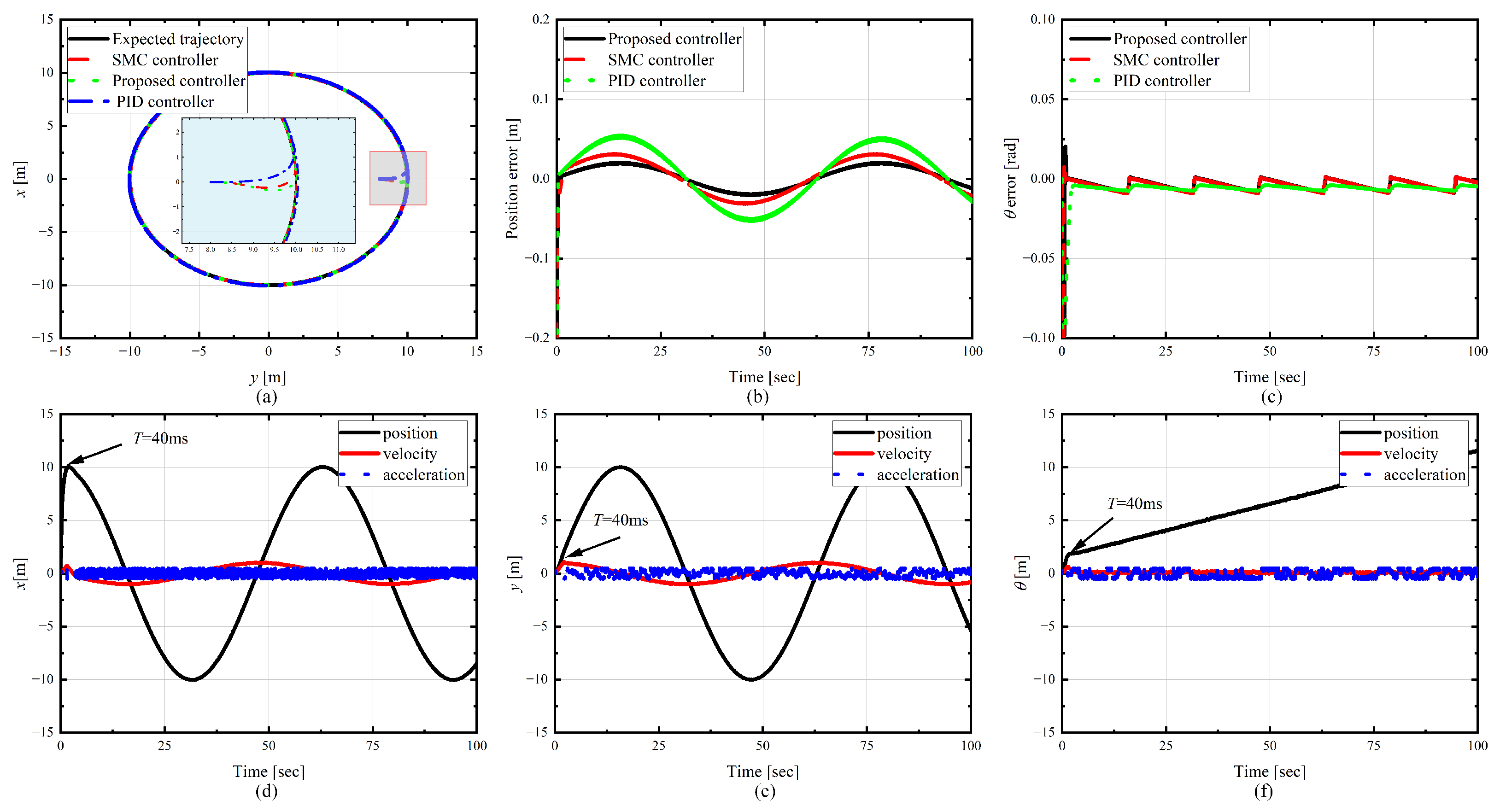
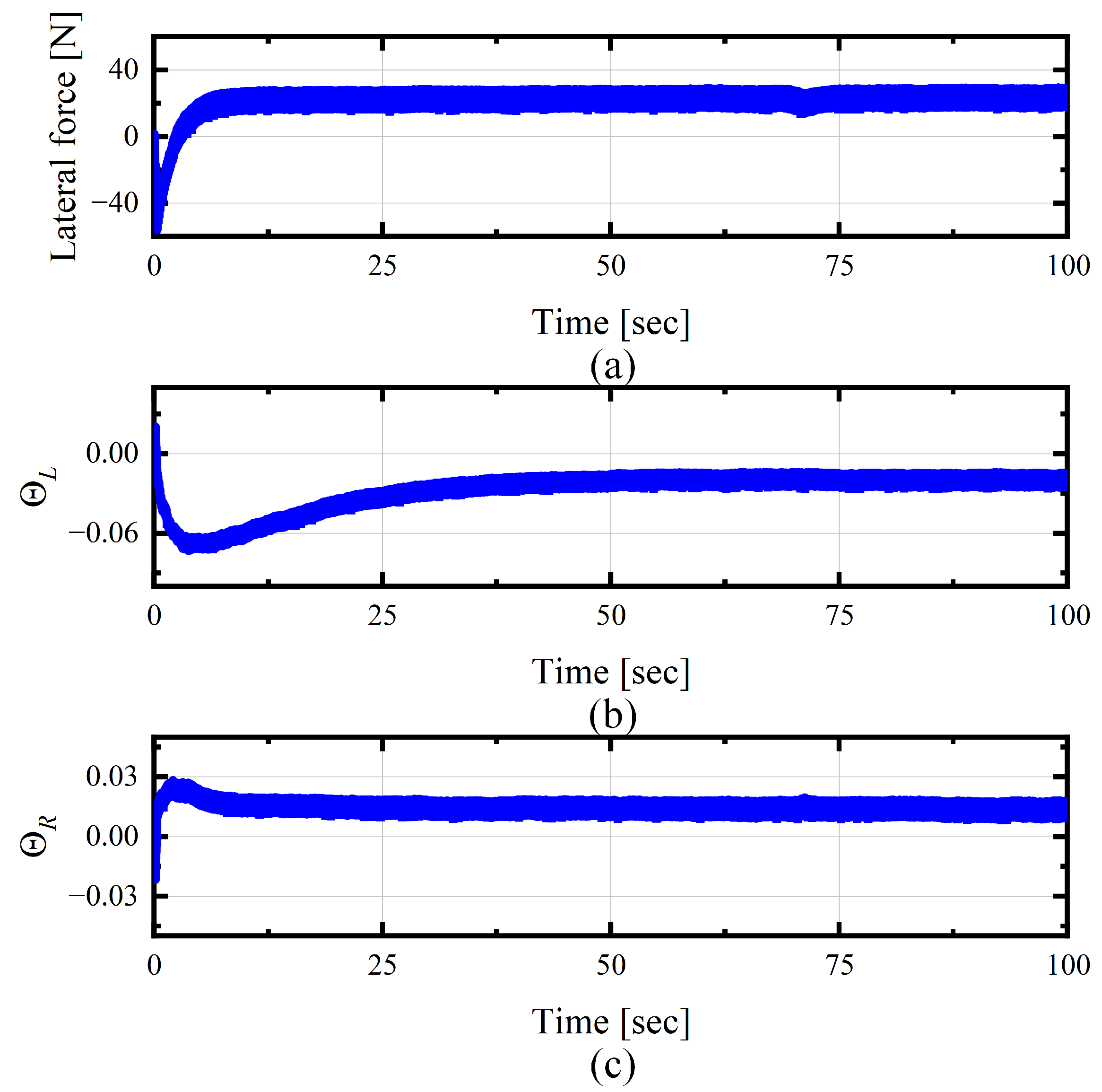
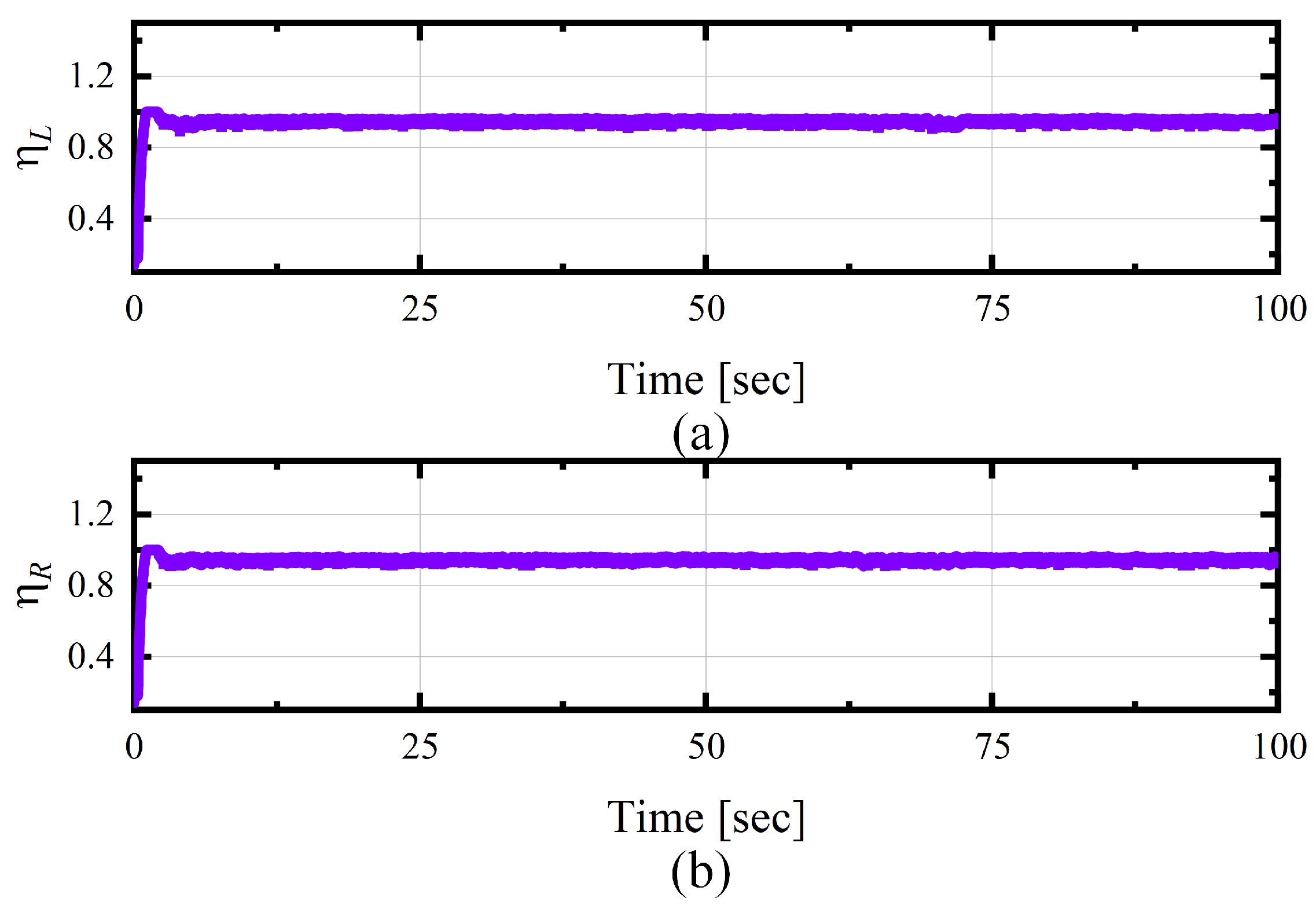
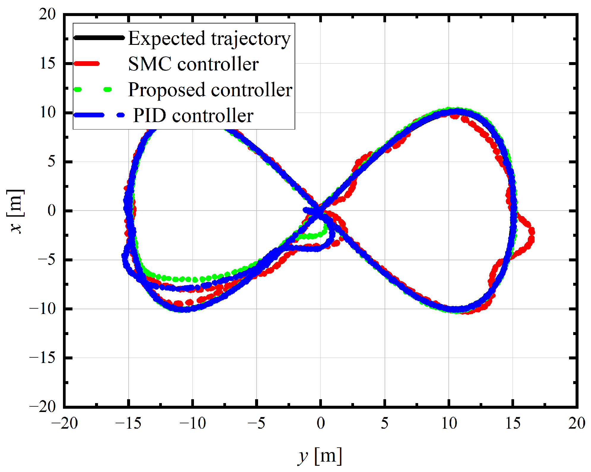
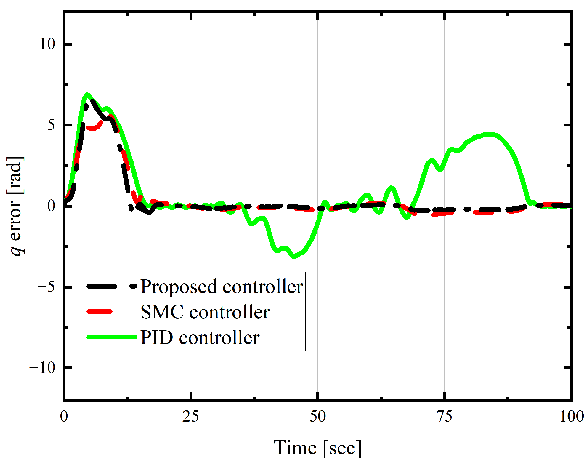
The experimental results verified the effectiveness of the proposed scheme. Even in the presence of both sensor and actuator faults, the trajectory tracking error remained within 0.1 m, while the error of the PID controller exceeded 0.4 m, and the error of the SMC controller was about 0.2 m. The actuator fault observer could accurately estimate power loss factors, providing necessary compensation information for the controller.

This research has significant implications for improving the reliability and safety of mining tracked mobile vehicles in harsh environments. The proposed distributed observation and fixed-time fault-tolerant control methods can also be extended to other non-holonomic constraint systems. It should be noted that this method also has certain potential limitations: bi-power sliding mode parameters need precise adjustment according to specific application scenarios, and inappropriate parameter selection may cause system oscillation; when sensors completely fail without redundant configuration, signal reconstruction capability is limited; and under extreme terrain conditions, LPV model accuracy may decrease. These limitations point to improvement directions for future research. Future work will further investigate fault-tolerant strategies under multiple coupled fault conditions, as well as controller design problems considering more complex terrain conditions. Moreover, the proposed methodology demonstrates broader applicability across multiple domains. The parameter-dependent LPV modeling framework can potentially be generalized to other nonlinear systems characterized by time-varying parameters. The hierarchical unknown input observer structure provides a systematic approach for managing high-dimensional system complexities. The fixed-time control methodology utilizing dual-power sliding mode surfaces offers theoretical guarantees suitable for applications requiring deterministic convergence properties. Therefore, with appropriate parameter tuning, the proposed system architecture may be transferable to diverse applications, including agricultural machinery and industrial production environments.

References

1. Ye, F.; Su, Y. Research on modeling and control algorithm of self-balancing platform of spraying robot. J. Phys. Conf. Ser. 2023, 2437, 012109. [Google Scholar] [CrossRef]
2. Du, G.; Zou, Y.; Zhang, X.; Guo, L.; Guo, N. Energy management for a hybrid electric vehicle based on prioritized deep reinforcement learning framework. Energy 2022, 241, 122523. [Google Scholar] [CrossRef]
3. Febbraro, A.; Dutto, M.; Bascetta, L.; Ferretti, G. Object-oriented modelling of a tracked vehicle for agricultural applications. Comput. Electron. Agric. 2025, 230, 109921. [Google Scholar] [CrossRef]
4. Zou, T.; Angeles, J.; Hassani, F. Dynamic modeling and trajectory tracking control of unmanned tracked vehicles. Robot. Auton. Syst. 2018, 110, 102–111. [Google Scholar] [CrossRef]
5. Chen, Y.; Zhang, H.; Zou, W.; Zhang, H.; Zhou, B.; Xu, D. Dynamic modeling and learning based path tracking control for ROV-based deep-sea mining vehicle. Expert Syst. Appl. 2025, 262, 125612. [Google Scholar] [CrossRef]
6. Cho, S.G.; Park, S.; Oh, J.; Min, C.; Kim, H.; Hong, S.; Jang, J.; Lee, T.H. Design optimization of deep-seabed pilot miner system with coupled relations between constraints. J. Terramechanics 2019, 83, 25–34. [Google Scholar] [CrossRef]
7. Huang, Y.; Xu, X.; Li, Y.; Zhang, X.; Liu, Y.; Zhang, X. Vehicle-following control based on deep reinforcement learning. Appl. Sci. 2022, 12, 10648. [Google Scholar] [CrossRef]
8. Luo, H.; Duan, J.; Wang, G. Mathematical Models for Truck-Drone Routing Problem: Literature Review. Appl. Math. Model. 2025, 114, 116074. [Google Scholar] [CrossRef]
9. Subari, M.A.; Hudha, K.; Kadir, Z.A.; Dardin, S.M.F.B.S.M.; Amer, N.H. Development of path tracking control of a tracked vehicle for an unmanned ground vehicle. Int. J. Adv. Mechatron. Syst. 2020, 8, 136–143. [Google Scholar] [CrossRef]
10. Yang, J.; Wu, Y. Observer-based adaptive control for uncertain nonholonomic systems subject to time-varying function constraints on states. Nonlinear Dyn. 2024, 113, 10175–10190. [Google Scholar] [CrossRef]
11. Wang, X.; Wang, Y.; Sun, Q.; Chen, Y.; Al-Zahran, A. Adaptive robust control of unmanned tracked vehicles for trajectory tracking based on constraint modeling and analysis. Nonlinear Dyn. 2024, 112, 9117–9135. [Google Scholar] [CrossRef]
12. Endo, D.; Okada, Y.; Nagatani, K.; Yoshida, K. Path following control for tracked vehicles based on slip-compensating odometry. In Proceedings of the 2007 IEEE/RSJ International Conference on Intelligent Robots and Systems, San Diego, CA, USA, 29 October–2 November 2007; IEEE: Piscataway, NJ, USA, 2007; pp. 2871–2876. [Google Scholar]
13. Burke, M. Path-following control of a velocity constrained tracked vehicle incorporating adaptive slip estimation. In Proceedings of the 2012 IEEE International Conference on Robotics and Automation, St Paul, MN, USA, 14–18 May 2012; IEEE: Piscataway, NJ, USA, 2012; pp. 97–102. [Google Scholar]
14. Kanayama, Y.; Kimura, Y.; Miyazaki, F.; Noguchi, T. A Stable Tracking Control Method for a Non-Holonomic Mobile Robot; IEEE: Osaka, Japan, 1991. [Google Scholar]
15. Zhou, B.; Peng, Y.; Han, J. UKF based estimation and tracking control of nonholonomic mobile robots with slipping. In Proceedings of the 2007 IEEE International Conference on Robotics and Biomimetics (ROBIO), Sanya, China, 15–18 December 2007; IEEE: Piscataway, NJ, USA, 2007; pp. 2058–2063. [Google Scholar]
16. Martínez, J.L.; Mandow, A.; Morales, J.; Garcia-Cerezo, A.; Pedraza, S. Kinematic modelling of tracked vehicles by experimental identification. In Proceedings of the 2004 IEEE/RSJ International Conference on Intelligent Robots and Systems (IROS) (IEEE Cat. No. 04CH37566), Sendai, Japan, 28 September–2 October 2004; IEEE: Piscataway, NJ, USA, 2004; Volume 2, pp. 1487–1492. [Google Scholar]
17. Balamurugan, S.; Srinivasan, R. Tracked vehicle performance evaluation using multi body dynamics. Def. Sci. J. 2017, 67, 476. [Google Scholar] [CrossRef]
18. Sabiha, A.D.; Kamel, M.A.; Said, E.; Hussein, W.M. Dynamic modeling and optimized trajectory tracking control of an autonomous tracked vehicle via backstepping and sliding mode control. Proc. Inst. Mech. Eng. Part I J. Syst. Control Eng. 2022, 236, 620–633. [Google Scholar] [CrossRef]
19. Conejo, C.; Puig, V.; Morcego, B.; Navas, F.; Milanés, V. Enhancing safety in autonomous vehicles using zonotopic LPV-EKF for fault detection and isolation in state estimation. Control Eng. Pract. 2025, 156, 106192. [Google Scholar] [CrossRef]
20. Dong, H.; Yu, H.; Xi, J. Phase portrait analysis and drifting control of unmanned tracked vehicles. IEEE Trans. Intell. Veh. 2024, 9, 5650–5664. [Google Scholar] [CrossRef]
21. Li, Z.; Wang, W.; Zhang, C.; Zheng, Q.; Liu, L. Fault-tolerant control based on fractional sliding mode: Crawler plant protection robot. Comput. Electr. Eng. 2023, 105, 108527. [Google Scholar] [CrossRef]
22. Fu, M.; Li, M.; Xie, W. Finite-time trajectory tracking fault-tolerant control for surface vessel based on time-varying sliding mode. IEEE Access 2017, 6, 2425–2433. [Google Scholar] [CrossRef]
23. Gáspár, P.; Szabó, Z.; Bokor, J. LPV design of fault-tolerant control for road vehicles. In Proceedings of the 2010 Conference on Control and Fault-Tolerant Systems (SysTol), Nice, France, 6–8 October 2010; IEEE: Piscataway, NJ, USA, 2010; pp. 807–812. [Google Scholar]
24. Li, B.; Du, H.; Li, W. Fault-tolerant control of electric vehicles with in-wheel motors using actuator-grouping sliding mode controllers. Mech. Syst. Signal Process. 2016, 72, 462–485. [Google Scholar] [CrossRef]
25. Dai, H.; Chen, P.; Yang, H. Metalearning-based fault-tolerant control for skid steering vehicles under actuator fault conditions. Sensors 2022, 22, 845. [Google Scholar] [CrossRef]
26. Xi, Z.J.; Hong, Y.G. Fault-Tolerant Fixed-Time Trajectory Tracking Control of Autonomous Surface Vessels with Specified Accuracy. IEEE Trans. Ind. Electron. 2020, 67, 4889–4899. [Google Scholar]
27. Geng, K.; Chulin, N.A.; Wang, Z. Fault-tolerant model predictive control algorithm for path tracking of autonomous vehicle. Sensors 2020, 20, 4245. [Google Scholar] [CrossRef] [PubMed]
28. Wong, J.Y. Theory of Ground Vehicles; John Wiley & Sons: Hoboken, NJ, USA, 2022. [Google Scholar]
29. Zhu, Y.; Xu, Z. A method of LPV model identification for control. IFAC Proc. Vol. 2008, 41, 5018–5023. [Google Scholar] [CrossRef]
30. Chen, M.; Wang, H.; Liu, X. Adaptive fuzzy practical fixed-time tracking control of nonlinear systems. IEEE Trans. Fuzzy Syst. 2019, 29, 664–673. [Google Scholar] [CrossRef]
31. Jiang, Y.; Wang, Q.; Chen, G.; Wu, Z. Sliding mode fault-tolerant control for nonlinear high-order fully actuated systems. IEEE Trans. Cybern. 2024, 55, 184–193. [Google Scholar] [CrossRef]
32. Levant, A. Higher-order sliding modes, differentiation and output-feedback control. Int. J. Control 2003, 76, 924–941. [Google Scholar] [CrossRef]
33. Hunter, S.K.; Pereira, H.M.; Keenan, K.G. The aging neuromuscular system and motor performance. J. Appl. Physiol. 2016, 121, 982–995. [Google Scholar] [CrossRef]
34. Yan, X.; Wang, S.; He, Y.; Ma, A.; Zhao, S. Autonomous Tracked Vehicle Trajectory Tracking Control Based on Disturbance Observation and Sliding Mode Control. Actuators 2025, 14, 51. [Google Scholar] [CrossRef]
Figure 1. TMV experimental testing platform.
Actuators 14 00330 g001
Figure 2. TMV steering diagram.
Actuators 14 00330 g002
Figure 3. Fault-tolerant control system structure diagram.
Actuators 14 00330 g003
Figure 4. Basic trajectory tracking test results, where (a) trajectory tracking curve, (b) pose tracking error curve, (c) yaw angle tracking error curve, (d) fixed-time differentiator estimate X direction projection curve, (e) fixed-time differentiator estimate Y direction projection curve, and (f) fixed-time differentiator estimate θ direction projection curve.
Actuators 14 00330 g004
Figure 5. Disturbance estimation distribution curves, where (a) lateral force estimate, (b) left wheel slip rate estimate, (c) right wheel slip rate estimate.
Actuators 14 00330 g005
Figure 6. Motor power loss factor estimation distribution curves, where (a) is the left-side motor power loss factor estimate and (b) is the right-side motor power loss factor estimate.
Actuators 14 00330 g006
Figure 7. Fault state trajectory tracking test results, where (a) sensor fault trajectory tracking curve, (b) sensor fault pose tracking error, (c) sensor fault heading angle tracking error, (d) trajectory tracking error under actuator fault, (e) pose tracking error under actuator fault, (f) heading angle tracking error under actuator fault.
Actuators 14 00330 g007
Figure 8. Power loss factor observation curves under actuator fault conditions, where (a) is the left-side motor power loss factor estimate and (b) is the right-side motor power loss factor estimate.
Actuators 14 00330 g008
Figure 9. Figure-eight desired trajectory tracking test results.
Actuators 14 00330 g009
Figure 10. Figure-eight desired trajectory tracking error distribution.
Actuators 14 00330 g010
Disclaimer/Publisher’s Note: The statements, opinions and data contained in all publications are solely those of the individual author(s) and contributor(s) and not of MDPI and/or the editor(s). MDPI and/or the editor(s) disclaim responsibility for any injury to people or property resulting from any ideas, methods, instructions or products referred to in the content.