A Computational Intelligence-Based Proposal for Cybersecurity and Health Management with Continuous Learning in Chemical Processes

Abstract

Ensuring cybersecurity and health management is a fundamental requirement in modern chemical industry plants operating under the Industry 4.0 framework. Traditionally, these two concerns have been addressed independently, despite sharing multiple underlying elements which suggest the viability of a unified detection and localization solution. This study introduces a computational intelligence framework based on fuzzy techniques, which allows for the early identification and precise localization of both faults and cyberattacks, along with the capability to recognize previously unseen events during runtime. Once new events are identified and classified, the training database is updated, creating a mechanism for continuous learning. This integrated approach simplifies the computational complexity of supervisory systems and enhances collaboration between the Operational Technology and Information Technology teams within chemical plants. The proposed methodology demonstrates strong robustness and reliability, even in complex conditions characterized by noisy measurements and disturbances, achieving outstanding performance due to its excellent discrimination capabilities.

1. Introduction

Contemporary terms such as “smart manufacturing”, “smart factories”, and “Industry 4.0” are closely intertwined with the automation of industrial operations. These systems are distinguished by their increasing interconnectivity and the extensive adoption of digital technologies across various processes [1,2]. This growing interconnection leads to enhanced efficiency, superior productivity, winning end products, and strict conformity with safety regulations in manufacturing. However, realizing these significant commercial benefits also amplifies two major risks that demand immediate attention: the challenges of industrial cybersecurity [3,4,5,6] and the potential occurrence of faults, both of which adversely impact safety, efficiency, and operational costs [7,8,9,10,11,12].

To mitigate these risks, it is essential that industrial plants employ condition-monitoring systems capable of early detection and accurate localization of cyber threats and operational anomalies. This necessity has driven a significant body of research in recent years, focused on developing methods for monitoring the operational conditions of industrial systems [13,14,15]. Achieving high diagnostic accuracy requires correctly classifying the operational modes of the plant, which is a complex task due to the uncertainties introduced by measurement noise and system disturbances.

In scientific literature, methods for detecting and localizing faults and cyberattacks are generally classified as either model-based or data-driven approaches [14,15,16,17]. Model-based methods rely on deep knowledge of the system, including its parameters and operating modes, to ensure accurate detection. However, the complexity of modern industrial facilities makes it difficult to obtain such comprehensive process knowledge. On the other hand, data-driven methods offer an alternative that eliminates the need for an explicit mathematical model or detailed prior understanding of the system’s variables and their relationships [18,19,20,21,22]. The evolution of technologies such as the Internet of Things (IoT) and Big Data analytics has greatly advanced this data-driven approach, producing valuable results in industrial applications [23,24].

Recent analyses of condition-monitoring strategies highlight the increasing use of fuzzy logic techniques [25,26,27]. Fuzzy clustering methods are especially well suited to handling the ambiguity and uncertainty common in many real-world applications. A notable strength of fuzzy set theory is its use of membership degrees to represent the association between elements and classes. Recent developments have introduced Type-2 fuzzy sets, which extend this concept by more effectively representing and handling the uncertainty and imprecision inherent in membership functions [28,29].

A review of the current research landscape reveals that health management and cybersecurity are still often addressed separately. Faults in industrial systems are typically caused by physical degradation due to wear or by unintentional operational errors. Fault diagnosis has been studied for over four decades and traditionally falls within the responsibility of the operational technology (OT) domain. The authors in [23] review current advances in knowledge base construction using ontologies and deductive/inductive reasoning for knowledge-based fault diagnosis. These approaches improve interoperability, providing greater reasoning and answers to queries for non-expert users. Other methods address Intelligent Fault Diagnosis (IFD) in industrial applications. The work presented in [30] proposes a new Heterogeneous Signal Integration (HSE) module that projects these types of signals in a unified space, providing integration with IFD architectures. In contrast, cybersecurity challenges emerged later, as physical plants evolved into cyber-physical systems. Cyberattacks generally result from malicious actions aimed at inducing catastrophic failures and are typically controlled by information technology (IT) teams. In [5], an Early Warning System based on Informed Physics is proposed. This approach enables real-time detection of cyberattacks in Industrial Control Systems. The authors in [16] conduct a study on cyberattacks based on auto-encoders trained online for multivariate time series. The method is validated using real data from an Industrial Control System.

However, with the rapid development of enabling technologies such as the Industrial Internet of Things, Cloud Computing, and Artificial Intelligence, the line between OT and IT is becoming increasingly blurred. This convergence has highlighted the need for closer collaboration between these two traditionally separate domains. One of the key insights from this integration is that the detection and localization of both faults and cyberattacks fall within the common goals of condition-monitoring systems, reinforcing the importance of developing unified methodologies for both issues [31]. For example, in [32], an integrated system for diagnosing faults and cyberattacks in industrial control systems is proposed. This approach proposes models of the industrial process for normal operating conditions and a fault isolation system based on expert knowledge of the relationship between faults and signs and symptoms, to detect and locate anomalies. On the other hand, the method proposed in [33] focuses on fault detection for network systems when they are subject to deception attacks. The proposed scheme introduces a filter as a residual generator to detect an occurring fault early, taking into account network delay and potential deception attacks. In [34], a system is proposed that provides real-time information on known and unknown types of attacks and faults in cyber-physical systems. This scheme also provides information on the occurrence, location, root cause, and physical impact of the anomalies that occurred in the process. However, none of these works address the problem of detecting new events.

In this article, we propose a novel condition-monitoring approach that uses Type-2 fuzzy logic techniques to jointly address fault diagnosis and cyberattack detection in chemical processes. The core contribution of this study is a robust monitoring framework that can withstand external noise and disturbances while reliably identifying and localizing both faults and cyberattacks. The proposed system employs Type-2 Fuzzy Sets and a Fuzzy Inference System (FIS), while a kernel-based extension is introduced to reduce classification errors and improve cluster separability. Additionally, the approach integrates the Density-Oriented Fuzzy C-Means (DOFCM) algorithm to detect new classes—whether they are previously unseen faults or cyberattacks—and automatically updates the training set, creating a continuous learning loop. Experimental validation confirms the robustness and effectiveness of the suggested strategy, even when data obtained from the process are affected by significant noise.

This paper is organized as follows: Section 2 introduces the core concepts and characteristics of the fuzzy clustering techniques employed. Section 3 details the proposed strategy for unified cybersecurity and health management with continuous learning, including the Type-2 fuzzy classifier, FIS, and DOFCM algorithm. Section 4 and Section 5 present case studies based on the Tennessee Eastman (TE) benchmark process, including the experimental design, results, and comparisons with other condition-monitoring algorithms. Finally, Section 6 provides the conclusions drawn from the study.

2. Understanding Fuzzy Clustering: Core Features

2.1. Fuzzy C-Means (FCM)

Over time, numerous fuzzy clustering algorithms have been proposed, one of the most widely used being the Fuzzy C-Means (FCM) algorithm. This technique partitions data into clusters by minimizing an objective function (1), which measures the similarity among data points based on their distance to cluster centers.

$$J_{FCM}={\displaystyle \sum _{j=1}^g}{\displaystyle \sum _{l=1}^M}{\displaystyle {\mu }_{jl}^f}{\displaystyle d_{jl}^2}\left({\mathbf{X}}_l,{\mathbf{V}}_j\right)$$

(1)

where ${\mathit{X}}_l=\left(\begin{array}{ccc}{x}_1,& \cdots & {,x}_M\end{array}\right)$ represents the set of data points and ${\mathit{V}}_j=\left(\begin{array}{ccc}{v}_1,& \cdots & {,v}_g\end{array}\right)$ represents the set of cluster centers.

The fuzziness of the resulting partition is influenced by the parameter f, where f > 1. As $f \to \infty ,$ membership degrees across clusters equalize, as $f \to 1$ patterns will exclusively pertain to a unique classification. Employing fuzzy clustering, the membership degrees of the matrix $U={[{\mu }_{jl}]}_{g\times M}$ can be obtained, with ${\mu }_{jl}$ representing the fuzzy membership degree of sample (l) to the j-th class, adhering to the subsequent condition:

$${\displaystyle \sum _{j=1}^g}{\mu }_{jl}=1, l=1, 2,\dots ,M$$

(2)

Here, g represents the number of categories, and M indicates the number of samples. The distance function $d_{jl}$, defined in Equation (3), is utilized to determine similarity. This function calculates the distance from each sample to the cluster centers, where $\mathit{A} \in {\mathfrak{R}}^{n\times n}$ refers to the norm induction matrix, and n denotes the number of measured features.

$${\displaystyle d_{jl}^2}={({\mathit{x}}_l-{\mathit{v}}_j)}^T\mathit{A}({\mathit{x}}_l-{\mathit{v}}_j)$$

(3)

The dissimilarity is assessed by calculating the squared distance between each sample and the cluster center, identified as ${\mathit{v}}_j$. Minimizing Equation (1) subject to the constraint set out in Equation (2) produces

$${\mu }_{jl}={\displaystyle \frac{1}{{\displaystyle {\sum }_{h=1}^g}{\left(\raisebox{1ex}{$d_{jl, \mathit{A}}$}\!\left/ \!\raisebox{-1ex}{$d_{hl,\mathit{A}}$}\right.\right)}^{\raisebox{1ex}{$2$}\!\left/ \!\raisebox{-1ex}{$(f-1)$}\right.}}}$$

(4)

$${\mathit{v}}_j={\displaystyle \frac{{\displaystyle {\sum }_{k=l}^M}{\left({\mu }_{jl}\right)}^f{\mathit{x}}_f}{{\displaystyle {\sum }_{l=1}^M}{\left({\mu }_{jl}\right)}^f}}$$

(5)

In Equation (5), ${\mathit{v}}_j$ denotes the weighted mean of the samples associated with a specific cluster center. The Fuzzy C-Means (FCM) procedure is repetitive and categorizes M data points into g groups. Initially, it is required to determine the number of patterns (g), which are initially selected at random and later adjusted throughout the process. The matrix U is updated iteratively until convergence is reached, as specified by the following condition: $‖U_t-U_{t-1}‖<\lambda$, where $\lambda$ denotes a previously defined threshold.

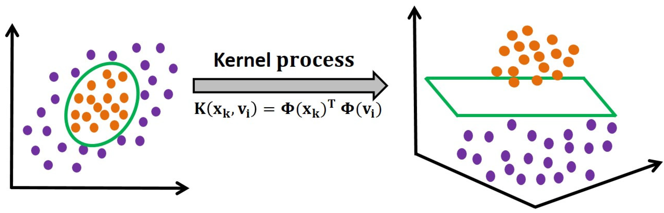
2.2. Kernel Fuzzy C-Means

Method kernels play an essential part in transforming non-linear data from the input space into a space with higher dimensionality (refer to Figure 1). The Kernelized Fuzzy C-Means Algorithm (KFCM) presents particular benefits for classification by enhancing the distinction between groups and, consequently, reducing classification errors. This advantage originates from modifying the objective function of FCM by means of o $\mathit{\psi }$, a mapping described as follows:

$$J_{KFCM}={\displaystyle \sum _{j=1}^g}{\displaystyle \sum _{l=1}^M}{\left({\mu }_{jl}\right)}^f{‖\mathit{\psi }({\mathit{x}}_l)-\mathit{\psi }({\mathit{v}}_j)‖}^2$$

(6)

Here, ${‖\mathit{\psi }({\mathit{x}}_l)-\mathit{\psi }({\mathit{v}}_j)‖}^2$ indicates the squared distance between $\mathit{\psi }({\mathit{x}}_{\mathit{l}})$ and $\mathit{\psi }\left({\mathit{v}}_{\mathit{j}}\right)$. This parameter is computed in the feature space utilizing a kernel function within the input space, defined as

$${‖\mathit{\psi }({\mathit{x}}_l)-\mathit{\psi }({\mathit{v}}_j)‖}^2=\mathit{K}({\mathit{x}}_l,{\mathit{x}}_l)-2\mathit{K}({\mathit{x}}_k,{\mathit{v}}_j)+\mathit{K}({\mathit{v}}_l,{\mathit{v}}_j)$$

(7)

When applying the Gaussian kernel, then $\mathit{K}(\mathit{x},\mathit{x})=1$ and ${‖\mathit{\psi }({\mathit{x}}_l)-\mathit{\psi }({\mathit{v}}_j)‖}^2=2(1-\mathit{K}({\mathit{x}}_l,{\mathit{v}}_j))$. As a result, Equation (6) can be reformulated as

$$J_{KFCM}=2{\displaystyle \sum _{j=1}^g}{\displaystyle \sum _{l=1}^M}{\left({\mu }_{jl}\right)}^f{‖1-\mathit{K}\left({\mathit{x}}_l,{\mathit{v}}_j\right)‖}^2$$

(8)

where,

$$\mathit{K}({\mathit{x}}_l,{\mathit{v}}_j)={\mathit{e}}^{{\displaystyle \raisebox{1ex}{$-{‖{\mathit{x}}_{\mathit{k}}-{\mathit{v}}_{\mathit{j}}‖}^2$}\!\left/ \!\raisebox{-1ex}{${\mathit{\sigma }}^2$}\right.}}$$

(9)

Minimizing Equation (6) under the constraints presented in Equation (2) leads to

$${\mu }_{jl}={\displaystyle \frac{1}{{\displaystyle {\sum }_{h=1}^g}{\left(\frac{1-\mathit{K}({\mathit{x}}_l,{\mathit{v}}_j)}{1-\mathit{K}({\mathit{x}}_l,{\mathit{v}}_h)}\right)}^{\raisebox{1ex}{$1$}\!\left/ \!\raisebox{-1ex}{$(f-1)$}\right.}}}$$

(10)

$${\mathit{v}}_j={\displaystyle \frac{{\displaystyle {\sum }_{k=l}^M}{\left({\mu }_{jl}\right)}^f\mathit{K}({\mathit{x}}_l,{\mathit{v}}_j){\mathit{x}}_l}{{\displaystyle {\sum }_{l=1}^M}{\left({\mu }_{jl}\right)}^f\mathit{K}({\mathit{x}}_l,{\mathit{v}}_j)}}$$

(11)

Algorithm 1 outlines the KFCM procedure, where the variable is used to count the iterations.

Algorithm 1: Kernelized Fuzzy C-Means (KFCM)

Input: data X, number of classes g, parameters $\lambda >0, f>1, \sigma , I_{t_{max}}$ . Output: matrix U, class centers V. Assign random entries to matrix U during initialization. for $I_t=1 to{ I}_t=I_{t_{max}}do$   Update the centroid of every classification by using Equation (11).   Compute the distances based on Equation (7).   Update matrix U using Equation (10).   Verify if the following termination condition is satisfied: $‖U_t-U_{t-1}‖<\lambda \wedge I_t\ge I_{t_{max}}$ end for

2.3. Type-2 FCM Algorithm (T2FCM) and Its Kernel Variant (KT2FCM)

Type-2 fuzzy sets (T2FS) are introduced to overcome the challenges Type-1 fuzzy sets (T1FS) face in capturing uncertainty, particularly in measurement data affected by noise and external factors in industrial contexts. Unlike Type-1 sets that assign exact membership values, T2FS uses fuzzy numbers to express membership. This model assumes greater contributions from larger membership values when updating cluster centers. In the T2FCM approach, the center of each cluster is recalculated as a weighted average of all data points, based on Type-2 membership values (T2MSV) derived from

$$a_{jl}={\mu }_{jl}-{\displaystyle \frac{1-{\mu }_{jl}}{2}}$$

(12)

Here, ${\mu }_{jl}$ and $a_{jl}$ represent Type-1 (T1) and Type-2 (T2) memberships, respectively. The updated cluster centers in T2FCM use the newly obtained T2MSV derived from FCM. Figure 2 shows an illustration of the primary and secondary triangular membership functions (TMF).

To improve the precision of this approach, KT2FCM is applied. This algorithm aims to improve the separability between clusters, thus enhancing classification performance. The objective function to minimize is as follows:

$$J_{KT2FCM}={\displaystyle \sum _{j=1}^g}{\displaystyle \sum _{l=1}^M}{\displaystyle a_{jl}^{\ast f}}{‖\mathit{\psi }\left({\mathit{x}}_l\right)-\mathit{\psi }\left({\mathit{v}}_j\right)‖}^2$$

(13)

where ${‖\mathit{\psi }\left({\mathit{x}}_l\right)-\mathit{\psi }\left({\mathit{v}}_j\right)‖}^2$ is the squared distance between $\mathit{\psi }\left({\mathit{x}}_{\mathit{l}}\right)$ and $\mathit{\psi }\left({\mathit{v}}_{\mathit{j}}\right)$. The calculation of distance in the feature space is performed using a kernel function in the input space, described as:

$${‖\mathit{\psi }({\mathit{x}}_l)-\mathit{\psi }({\mathit{v}}_j)‖}^2=\mathit{K}({\mathit{x}}_l,{\mathit{x}}_l)-2\mathit{K}({\mathit{x}}_l,{\mathit{v}}_j)+\mathit{K}({\mathit{v}}_j,{\mathit{v}}_j)$$

(14)

Numerous kernel functions have been documented in the literature, and the optimal one depends on the context of application [20]. Nevertheless, the Gaussian Kernel Function (GKF) is the most widely utilized. When this kernel is adopted, $\mathit{K}(\mathit{x},\mathit{x})=1$ and ${‖\mathit{\psi }({\mathit{x}}_l)-\mathit{\psi }({\mathit{v}}_j)‖}^2=2(1-\mathit{K}({\mathit{x}}_l,{\mathit{v}}_j))$, and therefore Equation (13) becomes

$$J_{KFCM}=2{\displaystyle \sum _{j=1}^g}{\displaystyle \sum _{l=1}^M}{\displaystyle a_{jl}^{\ast f}}{‖1-\mathit{K}({\mathit{x}}_l,{\mathit{v}}_j)‖}^2$$

(15)

where,

$$\mathit{K}({\mathit{x}}_l,{\mathit{v}}_j)={\mathit{e}}^{{\displaystyle \raisebox{1ex}{$-{‖{\mathit{x}}_{\mathit{l}}-{\mathit{v}}_{\mathit{j}}‖}^2$}\!\left/ \!\raisebox{-1ex}{${\mathit{\sigma }}^2$}\right.}}$$

(16)

where σ represents the bandwidth and specifies the smoothness level of the GKF. If Equation (15) is minimized, it yields

$${\displaystyle a_{jl}^{\ast }}={\displaystyle \frac{1}{\sum _{h=1}^g{\left(\frac{1-\mathit{K}({\mathit{x}}_l,{\mathit{v}}_j)}{1-\mathit{K}({\mathit{x}}_l,{\mathit{v}}_h)}\right)}^{\raisebox{1ex}{$1$}\!\left/ \!\raisebox{-1ex}{$(f-1)$}\right.}}}$$

(17)

$${\mathit{v}}_j={\displaystyle \frac{\sum _{k=l}^M{({\displaystyle a_{jl}^{\ast }})}^f\mathit{K}({\mathit{x}}_l,{\mathit{v}}_j){\mathit{x}}_l}{\sum _{l=1}^M{({\displaystyle a_{jl}^{\ast }})}^f\mathit{K}({\mathit{x}}_l,{\mathit{v}}_j)}}$$

(18)

Algorithm 2 presents the KT2FCM procedure.

Algorithm 2: KT2FCM

Input: dataset X, number of classifications g, parameters $\lambda >0, f>1, \sigma , I_{t_{max}}$. Output: matrix U, class centers V. Assign random entries to matrix U during initialization. Compute A based on Equation (12). for $I_t=1 to{ I}_t=I_{t_{max}}do$   Revise the centroid of each classification using Equation (18).   Compute the distances based on Equation (14).   Update matrix A using Equation (17).   Verify if the termination condition is satisfied: $‖A_t-A_{t-1}‖<\lambda \wedge I_t\ge I_{t_{max}}$ end for

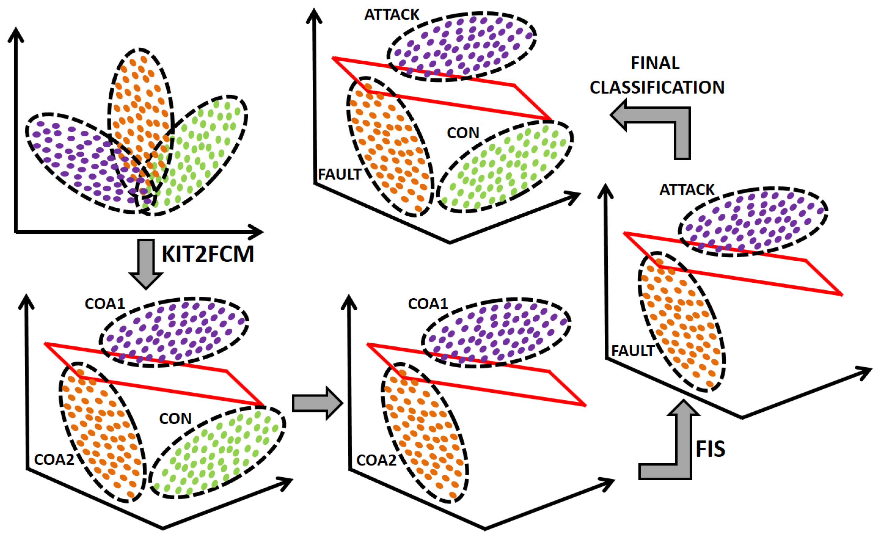
2.4. Interval Type-2 FCM (IT2FCM) and Its Kernel Variant (KIT2FCM)

The IT2FCM algorithm is crucial for its ability to robustly handle the uncertainty and imprecision inherent in real-world data. Unlike the T2FCM algorithm, IT2FCM provides more accurate and reliable clustering by directly modeling the imprecision of membership functions, making it especially valuable in complex and noisy environments. Figure 3 presents two interval T2FS. Figure 3a shows a fuzzy set determined by a TMF that has a mean me and a standard deviation within [σ₁, σ₂]. In Figure 3b, the standard deviation is fixed (σ), while the mean lies within [me1, me2]. The area between the curves represents the uncertainty in the primary membership of the Type-2 fuzzy set.

The Interval Type-2 Fuzzy C-Means algorithm (IT2FCM) treats the fuzzification coefficient as an interval $\left[f_1,f_2\right]$ [29]. It aims to minimize the following objective function:

$$J_{IT2FCM}={\displaystyle \sum _{j=1}^g}{\displaystyle \sum _{l=1}^M}{\left({\mu }_{jl}\right)}^f{\left(d_{jl}\right)}^2$$

(19)

In this expression, f is replaced by $f_1$ and $f_2$, which represent various degrees of fuzziness, yielding distinct objective functions compared to the conventional FCM algorithm. To carry out the minimization or maximization of the objective function, the following definitions are used:

$$\underset{\_}{{\mu }_j\left(l\right)}=min\left(\begin{array}{c}{\displaystyle \raisebox{1ex}{$1$}\!\left/ \!\raisebox{-1ex}{${\left({\displaystyle {\sum }_h^g}\raisebox{1ex}{$d_{jl}$}\!\left/ \!\raisebox{-1ex}{$d_{hl}$}\right.\right)}^{\raisebox{1ex}{$2$}\!\left/ \!\raisebox{-1ex}{$\left(f_1-1\right)$}\right.},$}\right.}\\ {\displaystyle \raisebox{1ex}{$1$}\!\left/ \!\raisebox{-1ex}{${\left({\displaystyle {\sum }_h^g}\raisebox{1ex}{$d_{jl}$}\!\left/ \!\raisebox{-1ex}{$d_{hl}$}\right.\right)}^{\raisebox{1ex}{$2$}\!\left/ \!\raisebox{-1ex}{$\left(f_2-1\right)$}\right.}$}\right.}\end{array}\right)$$

(20)

$$\overline{{\mu }_j\left(l\right)}=max\left(\begin{array}{c}{\displaystyle \raisebox{1ex}{$1$}\!\left/ \!\raisebox{-1ex}{${\left({\displaystyle {\sum }_h^g}\raisebox{1ex}{$d_{jl}$}\!\left/ \!\raisebox{-1ex}{$d_{hl}$}\right.\right)}^{\raisebox{1ex}{$2$}\!\left/ \!\raisebox{-1ex}{$\left(f_1-1\right)$}\right.},$}\right.}\\ {\displaystyle \raisebox{1ex}{$1$}\!\left/ \!\raisebox{-1ex}{${\left({\displaystyle {\sum }_h^g}\raisebox{1ex}{$d_{jl}$}\!\left/ \!\raisebox{-1ex}{$d_{hl}$}\right.\right)}^{\raisebox{1ex}{$2$}\!\left/ \!\raisebox{-1ex}{$\left(f_2-1\right)$}\right.}$}\right.}\end{array}\right)$$

(21)

Here, ${\displaystyle d_{jl}^2}=‖x_l-v_j‖$ denotes the distance between the input patterns and the cluster centers, $x_l$ and $v_j$. The upper and lower membership functions (MF) for the input patterns $x_l$ and the cluster centers $v_j$ are defined accordingly, $\overline{{\mu }_j(l)} ({\mu }_j(l))$. The IT2FCM method yields an interval T2FS, which cannot be transformed into a crisp set directly via defuzzification. The initial step in managing this output is a type-reduction, where the centroid of the T2FS is calculated and reduced to a T1 fuzzy set. Following this, the interval-valued class centers are calculated using these T2 memberships, as expressed in Equation (22):

$$\widetilde{{\mathit{v}}_j}=\left[\widetilde{v_{j,1}},\widetilde{v_{j,2}}\right]=\sum _{{\mu }_{j1}}\cdots \sum _{{\mu }_{j1}}{\displaystyle \frac{1}{\frac{{\displaystyle {\sum }_{l=1}^M}{\displaystyle {\mu }_{jl}^{f^{\ast }}}{x}_l}{{\displaystyle {\sum }_{l=1}^M}{\displaystyle {\mu }_{jl}^{f^{\ast }}}}}}$$

(22)

where $f^{\ast }$ changes from $f_1$ to $f_2$.

Throughout the iterative procedure, both the upper and lower fuzzy partition matrices are used. These help in the estimation of the interval T1 fuzzy set $\left[\widetilde{v_{j,1}},\widetilde{v_{j,2}}\right]$ corresponding to the center of each cluster, as detailed in [29]. The final crisp center V can be calculated with Equation (23):

$$\mathit{V}={\displaystyle \frac{\left(v_1+v_2\right)}{2}}$$

(23)

To improve the accuracy of IT2FCM, its kernel variant KT2FCM is applied. This approach seeks to improve the separability between classes, achieving higher classification performance. The kernelized version, KIT2FCM can be obtained with a similar procedure to the one used for T2FCM. The Gaussian Kernel Function (GKF) calculates distances in the feature space by employing a kernel function on the input space. Algorithm 3 presents the steps for KIT2FCM.

Algorithm 3: KIT2FCM

Input: dataset X, number of classes g, parameters $\lambda >0, f_1\left(f_2\right)>1, \sigma , I_{t_{max}}$. Output: matrix U, class centers V. Assign random entries to the lower matrix $\underset{\_}{{\mathit{U}}_1}$ and upper $\overline{{\mathit{U}}_2}$ in the initialization for $I_t=1 to{ I}_t=I_{t_{max}}do$   Revise the centroid of each classification using Equation (11) for $\widetilde{v_1}$ and $\widetilde{v_2}$.   Compute the distances based on Equation (14).   Update $\underset{\_}{{\mathit{U}}_1}$ and $\overline{{\mathit{U}}_2}$ using Equation (10) for $\underset{\_}{{\mu }_j\left(l\right)}$ and $\overline{{\mu }_j\left(l\right)}$   Update the cluster centers: $\mathit{V}={\displaystyle \frac{\left(v_1+v_2\right)}{2}}$.   Type-reduce the interval Type-2 fuzzy partition matrix as $\mathit{U}={\displaystyle \frac{\left(U_1+U_2\right)}{2}}$.   Verify if the termination condition is satisfied: $‖U_t-U_{t-1}‖<\lambda \wedge I_t\ge I_{t_{max}}$ end for

2.5. Density-Oriented Fuzzy C-Means (DOFCM)

The Density-Oriented Fuzzy C-Means algorithm (DOFCM) is designed to reduce sensitivity to noise in fuzzy clustering through the identification of the outliers prior to executing the clustering operation. This is accomplished by forming g + 1 clusters—that is, g standard clusters plus one that is specifically assigned to noise. The method detects outliers by evaluating the density of the dataset.

Under this approach, a minimum number of neighbors is required within a specified radius around each point. A density measure called neighborhood membership is introduced to assess how compactly points are clustered locally. The local membership for a point i in dataset X is defined as

$${\displaystyle M_{neighborhood}^i}={\displaystyle \frac{{\displaystyle {\eta }_{neighborhood}^i}}{{\eta }_{max}}}$$

(24)

where ${\displaystyle {\eta }_{neighborhood}^i}$ represents the number of points within the neighborhood of point i, while ${\eta }_{max}$ denotes the maximum amount of neighboring points observed for any point in the dataset.

A point q is considered a neighbor of i (i.e., belongs to its neighborhood), if q fulfills the following condition:

$$q\in X | dist(i,q) \le r_{neighborhood}$$

(25)

Here, $r_{neighborhood}$ represents the radius of the neighborhood, and $dist(i,q)$ denotes the distance between the two points. The value for $r_{neighborhood}$ is calculated according to the approach in [35].

Using Equation (24), the neighborhood membership value is calculated for all points in X. The threshold α is subsequently chosen from the complete set of values, based on the density of the dataset. A point is classified as an outlier if its degree of neighborhood membership is less than α. For a particular point i in X, this condition is expressed as

$$\left\{\begin{array}{c}{\displaystyle M_{neighborhood}^i}<\alpha , then i is an outlier\\ {\displaystyle M_{neighborhood}^i}\ge \alpha , then i is not an outlier\end{array}\right.$$

(26)

If a point is isolated within the data space, its membership value should ideally approach zero. In theory, a point would be identified as an outlier only when no other points are nearby (indicating a membership of zero) or if α is set to zero. However, in this method, a point is considered an outlier if its neighborhood membership falls below the threshold α, which serves as a key parameter for outlier detection. The exact value of α is influenced by the dataset’s characteristics and typically varies with its density. Once the outliers have been detected, the clustering process continues as outlined in [35]. Algorithm 4, DOFCM is presented next.

Algorithm 4: DOFCM to determine the presence of a new class

Input: Dataset with outliers X, number of clusters c, Output: Filtered dataset without outliers Xp  Compute the neighborhood radius.  Compute ${\displaystyle {\mathsf{\eta }}_{\mathrm{n}\mathrm{e}\mathrm{i}\mathrm{g}\mathrm{h}\mathrm{b}\mathrm{o}\mathrm{r}\mathrm{h}\mathrm{o}\mathrm{o}\mathrm{d}}^{\mathrm{i}}}$ using Equation (25).  Determine ${\mathsf{\eta }}_{\mathrm{m}\mathrm{a}\mathrm{x}}$.  Compute ${\displaystyle {\mathrm{M}}_{\mathrm{n}\mathrm{e}\mathrm{i}\mathrm{g}\mathrm{h}\mathrm{b}\mathrm{o}\mathrm{r}\mathrm{h}\mathrm{o}\mathrm{o}\mathrm{d}}^{\mathrm{i}}}$ using Equation (24).  Using the specified value of $\mathsf{\alpha }$ , identify outliers according to Equation (26).

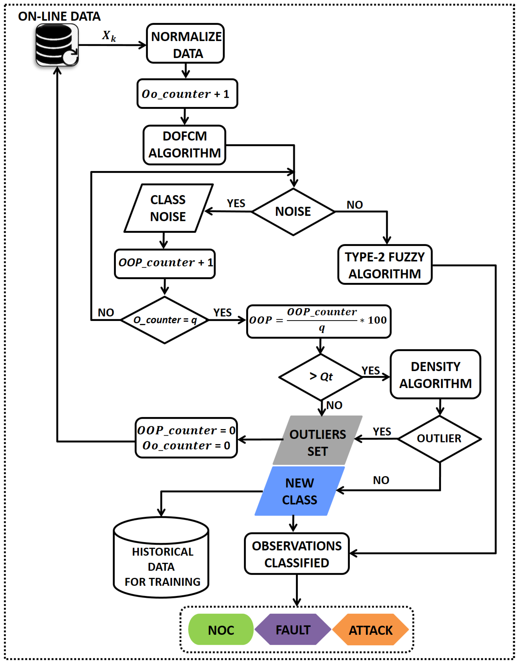
3. Proposed Monitoring Scheme

The monitoring approach developed for detecting cyberattacks and managing health with continuous learning is presented in Figure 4. The system has two stages: offline training and online analysis.

Initially, a dataset consisting of historical records from the chemical process is utilized to train a classifier. Once training is complete, the classifier is applied in real time to assess each new observation from the ongoing process. The training step is crucial, as it establishes the center for each classification, corresponding to different process conditions, either normal or involving faults and cyberattacks.

3.1. Offline Training

This phase involves training the classifier with historical data identifying the class centers ${\mathit{v}}_1,{\mathit{v}}_2,\dots ,{\mathit{v}}_{\mathit{M}}$. The g classes are representative of the Normal Operating Conditions (CON) for this process with several Abnormal Operating Conditions (COA) affecting it, even though uncertainty exists regarding whether these COAs derive from faults and/or cyberattacks. KIT2FCM maps the observed data in higher-dimensional space, minimizing errors in classification.

To determine whether the states categorized as COAs are caused by faults or cyberattacks, the system integrates a base of knowledge, implemented through a Fuzzy Inference System (FIS). The FIS assesses the variables that represent symptoms—those affected by the occurrence of faults or cyberattacks—and determines the nature of the anomaly influencing the process. It is crucial to emphasize that the symptom variables of the process should include not only the outputs but also the inputs. In many cases, attackers tamper with the process’s input parameters to imitate CON or specific fault conditions.

The evaluation of each symptom variable employs trapezoidal membership functions, as outlined in Equations (27)–(29). As depicted in Figure 5, fuzzy sets labeled Low (L), Normal (N), and High (H) are used to describe the conduct of each parameter $S_i$. Here, $X_{min},X_{max}$, and δ correspond to the minimum, maximum, and standard deviation values of the CON.

$${\mu }_{low}=\left\{\begin{array}{c}\begin{array}{cc}0& if S_i>X_{min}\end{array}\\ \begin{array}{cc}{\displaystyle \frac{X_{min}-S_i}{\delta }}& if \left(X_{min}-\delta \right)\le S_i\le X_{min}\end{array}\\ \begin{array}{cc}1& if S_i\le \left(X_{min}-\delta \right)\end{array}\end{array}\right.$$

(27)

$${\mu }_{normal}=\left\{\begin{array}{c}\begin{array}{cc}0& if S_i<\left(X_{min}-\delta \right)\end{array}\parallel S_i>\left(X_{max}+\delta \right)\\ \begin{array}{cc}{\displaystyle \frac{S_i-\left(X_{min}-\delta \right)}{\delta }}& if \left(X_{min}-\delta \right)\le S_i\le X_{min}\end{array}\\ \begin{array}{cc}{\displaystyle \frac{\left(X_{max}+\delta \right)-S_i}{\delta }}& if{ X}_{max}\le S_i\le \left(X_{max}+\delta \right)\end{array}\\ \begin{array}{cc}1& if X_{min}<S_i\le X_{max}\end{array}\end{array}\right.$$

(28)

$${\mu }_{high}=\left\{\begin{array}{c}\begin{array}{cc}0& if S_i<X_{max}\end{array}\\ \begin{array}{cc}{\displaystyle \frac{S_i-X_{max}}{\delta }}& if X_{max}\le S_i\le \left(X_{max}+\delta \right)\end{array}\\ \begin{array}{cc}1& if S_i>\left(X_{max}+\delta \right)\end{array}\end{array}\right.$$

(29)

A set of IF-THEN rules is subsequently developed to identify the type of abnormal condition influencing the process. The knowledge base is composed of rules based on expert insights and the behavior of process variables. Equation (30) illustrates a representative FIS rule.

$$\begin{gathered} IF \left(S_{1}is F{S}^i\right)AND\left(S_{2}is F{S}^i\right)AND\dots AND \left(S_{n}is F{S}^i\right) \\ THEN {COA}^j is Fault/Attack \end{gathered}$$

(30)

where,

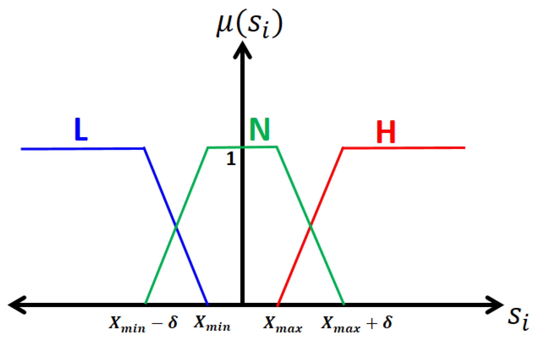
• n denotes the number of symptom variables in the process.
• i = 1 (FS low), 2 (FS normal), and 3 (FS high).
• j = 1 (Fault) and 2 (Attack)

Building a Knowledge Base requires a series of stages. As shown in Figure 6, this methodology can be scalable and applied to other industrial processes. The stages to follow are described below:

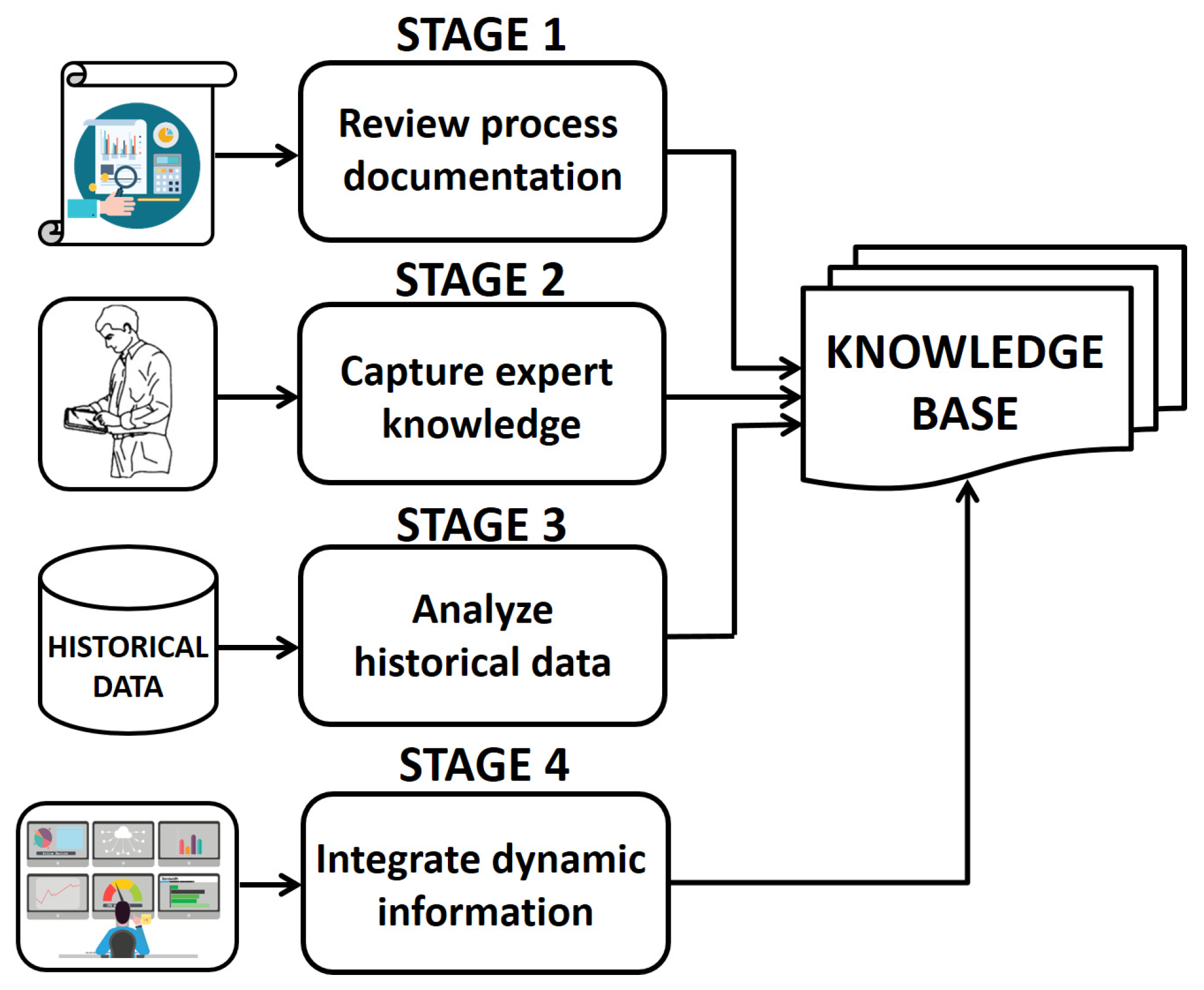
• Review process documentation: review manuals, standard operating procedures, safety protocols, repair records, previous incident reports, and design specifications.
• Capture expert knowledge: Conduct interviews with experts in the operation of the process; capture undocumented knowledge from experienced personnel through direct observation.
• Analyze historical data: Examine the most common problems with variable symptoms, common errors, and successful resolutions based on operational data and maintenance records.
• Integrate dynamic information: Integrate data from the monitoring system to feed the knowledge base with dynamic information.

Figure 7 summarizes the procedure followed during the training phase.

3.2. Online Analysis

Each observation (q) is classified in this step by evaluating its membership degree to all classes, determined by the distance to the class centers ($v_j$ f or j = 1, 2, …, g). It is then assigned to the class with the maximum membership value, as expressed in Equation (31).

$$C_j=\left\{j : max\left\{{\mu }_{jl}\right\}, \forall j,l\right\}$$

(31)

During this stage, the proposed approach supports the identification of new classes using a criterion based on data density. Alongside the classification of process observations, a mechanism is established for the recognition of new events. At this point, a panel of experts defines a time window containing q-observations and a threshold criterion designated as Qt. The value of q, determined based on the characteristics of the process, specifies the number of sampling intervals that experts consider adequate to assess the likelihood of a new event. Qt denotes the percentage of observations, also assigned by experts, required to determine whether the outlier instances within the q samples warrant further analysis to determine if they belong to a new class, potentially indicating the occurrence of a new event.

Upon receiving an observation $x_k$, KIT2FCM classifies it as normal operation, fault, attack, or outlier, depending on the outcome from the training phase. If $x_k$ is not labeled as an outlier, KIT2FCM identifies the known class it belongs to. However, if $x_k$ is categorized as an outlier, it is saved, and a counter variable for outlier observations (O_O) is incremented. The process continues until the window of q-observations is complete.

After processing all the q-observations, the outlier percentage (OOP = O_O × 100/q) is determined. If the OOP does not surpass Qt, the group of observations is not regarded as suggestive of a new class, and the O_O counter is reset to initiate a new cycle. When the OOP exceeds Qt, the O_O instances are examined to identify if they correspond to a new classification, possibly a new fault or attack, or whether they are true outliers.

A potential scenario where the new class corresponds to a different operating condition is not evaluated in this context. This is based on the assumption that such transitions are known to plant technicians and that the diagnostic system can be updated before the plant enters that condition.

The DOFCM algorithm is utilized to investigate outlier observations, based on the assumption that outliers are sparsely distributed and have low density, meaning they do not create a distinct, cohesive cluster. In contrast, when a new event (fault or attack) occurs, the data related to it tend to cluster tightly, signaling high density and forming a new state. DOFCM is employed with outlier observations to evaluate their density and decide whether they represent outliers or indicate the emergence of a new class.

Should the outlier data represent a new event, experts need to determine if the pattern is related to a fault, an attack, or a combination of the two. Once the identification and analysis of this new pattern are complete, and if the event is confirmed to be a new type of fault or attack, it is added to the historical dataset and used in the training phase. The classifier is then retrained, and the online diagnosis system is updated with the new fault detection capability. This full procedure is outlined in Algorithm 5. The described online analysis approach enables automatic detection of new faults or attacks, incorporating continuous learning into the cybersecurity and health management system. Figure 8 presents the detailed scheme of the online recognition stage with the detection of new events.

Algorithm 5: Online analysis

Input: data $X_i$, class centers V, f,  $\sigma , r_{neighborhood}$ , ${\eta }_{max}$ , $\alpha$ Output: Current State, New event Select q Select Qt Initialize OO counter = 0 Initialize OOP counter = 0 for $l=1 to l=q do$    Increment OO counter by 1    Compute ${\displaystyle {\eta }_{neighborhood}^i}$ using Equation (25)    Compute ${\displaystyle M_{neighborhood}^i}$ using Equation (24)    if q ≠ Coutlier then      Calculate the distances from the sample l to the class centers.      Calculate the membership degree of sample l to the g classes.      Assign observation l to a class according to Equation (31).    else      Store observation q in Cnoise      Increment the OOP counter by 1    end if end for Compute OOP = (OOP counter) x 100/q if OOP > Qt then    Apply the DOFCM algorithm for Cnoise assuming two classes (New Event, Outlier)    if Cnoise ≠ Coutlier then      Create a new pattern      Identify the new pattern: Fault or Attack      Store in the historical database for training    else      Delete Cnoise      Reset the OO counter and OOP counter to 0    end if    else      Delete Cnoise      Reset the OO counter and OOP counter to 0 end if

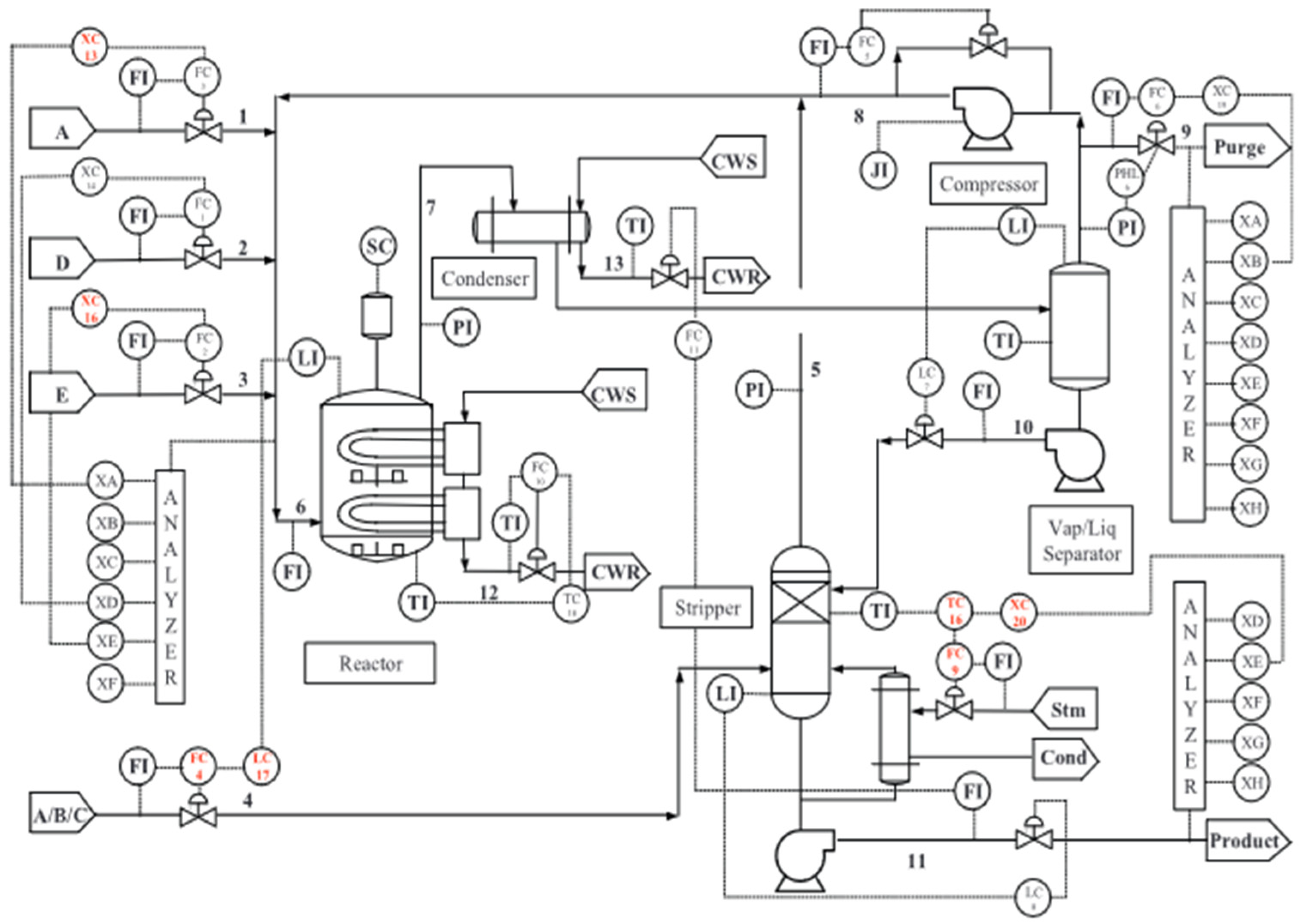
4. Case Study: Tennessee Eastman Process

4.1. Process Description

The Tennessee Eastman process (TEP) is employed here as a reference to evaluate the performance of the proposed condition-monitoring method [36,37]. The plant comprises five interconnected subsystems, as illustrated in Figure 9.

The figure illustrates that products G and H are generated from the reactants A, C, D, and E. The facility comprises five primary components: a reactor, a condenser, a vapor-liquid separator, a product stripper, and a compressor. The process involves 41 measured variables (VMe(1)–VMe(41)) and 12 manipulated variables (VMa(1)–VMa(12)).

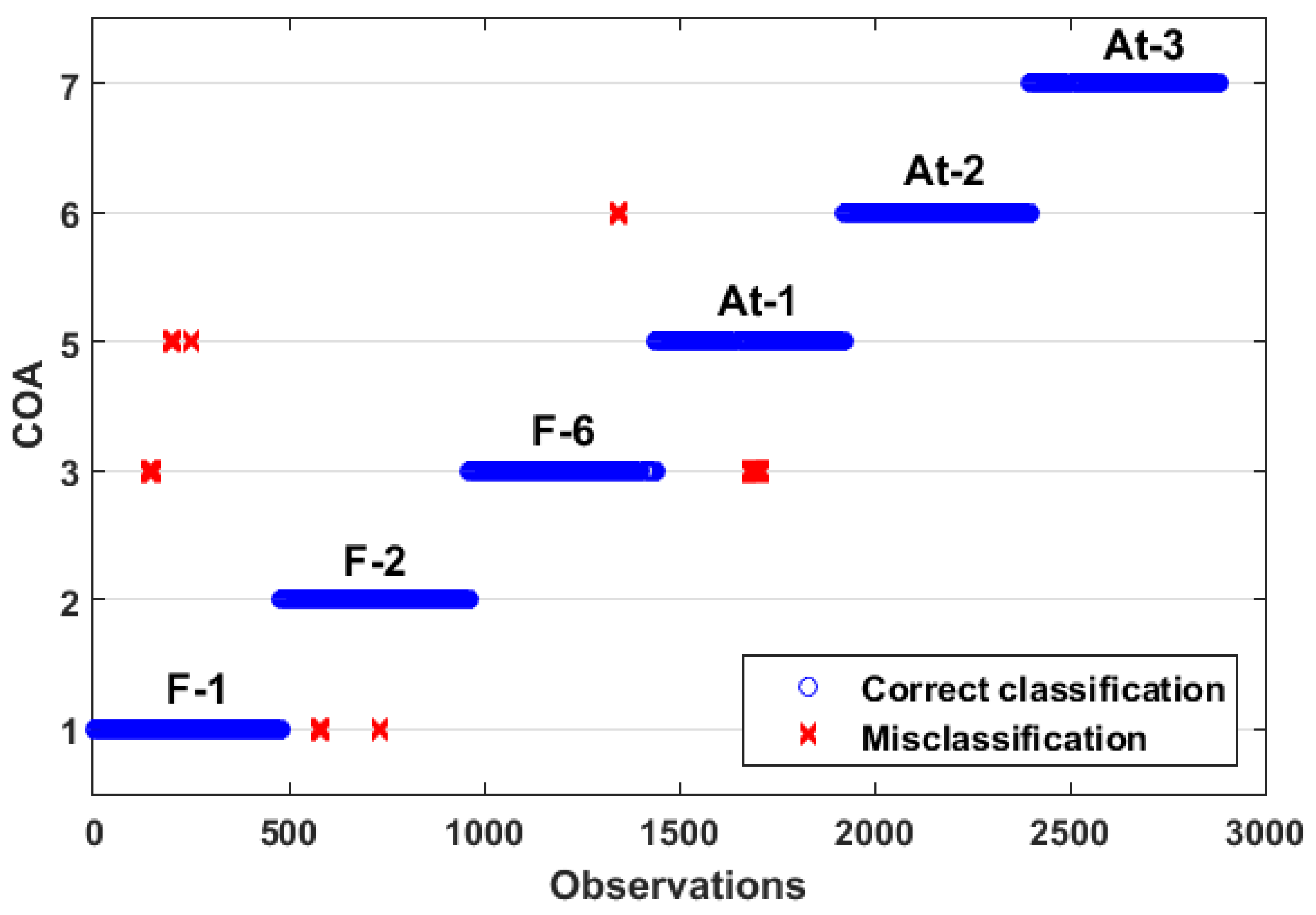
4.2. Experimental Design

This process includes sets of observations representing both the Normal Operating Condition and 21 distinct faults. Each dataset spans a 48-h period. The faults are introduced after the first 8 h of simulation. Noise is added to the datasets to assess the robustness of the proposed strategy.

Table 1. Faults examined in the TEP.

Fault	Process Variable	Type
Fault 1 (F-1)	A/C feed ratio, B composition constant	step
Fault 2 (F-2)	B composition, A/C ratio constant	step
Fault 6 (F-6)	A feed loss	step
Fault 7 (F-7)	C header pressure loss-reduced availability	step

lists the faults used for the evaluation and testing of the system. Initially, 480 samples were used for training for every fault and for the CON, followed by 960 samples in the online analysis stage.

Figure 10 displays the conduct of multiple symptom variables during the occurrence of Fault 6. While this fault may pose difficulties for the process operation, the system does not undergo a shutdown at any point. The following analysis will focus on the consequences of attacks on the process.

As detailed in

Table 2. Description of attacks on the Tennessee Eastman Process.

Type of Attack	Magnitude of the Sensor Under Attack	Symptom Variables	Description	Impact
Attack 1 (At-1)	VMe(1) [+2.35]	VMe(1), VMe(7), VMe(8), VMe(3)	For three hours, the actual value is incremented by a factor of 2.35	HRP or LSL: shutdown
Attack 2 (At-2)	VMe(14) [+7]	VMe(12), VMe(14), VMe(15), VMa(7), VMa(8)	For 2.88 h the actual value increases by 7	HSL: shutdown
Attack 3 (At-3)	VMe(14) [−7]	VMe(12), VMe(14), VMe(15), VMa(7), VMa(8)	For 2.02h the actual value decreases by 7	LSL: shutdown
Attack 4 (At-4)	VMe(14) [22.9]	VMe(12), VMe(15), VMa(7)	The value is set to 22.9 for 1.9 h	LSL: shutdown

VMe(1): A feed, VMe(7): Reactor pressure, VMe(8): Reactor level, VMe(14): Separator underflow, VMe(15): Stripper level, VMa(3): A feed flow, VMa(7): Separator flow, VMa(8): Stripper flow, High Reactor Pressure HRP, Low/High Stripper Level L/HSL, Low Separator Level LSL.

, the simulated attacks were first introduced in [11], where the attacker has complete knowledge of the process and the ability to modify sensor readings at any moment. Two attack types are examined: (a) deception attack, and (b) replay attack. The MATLAB R2024b simulation using the Simulink tool of the TEP described in [36] is used for the experiments. The simulated attacks are specified in Table 2. Similar to fault detection, 480 observations are utilized in the training phase, with 960 used for online analysis.

Figure 11 displays the occurrence of Attack 2. During the attack, the sensor reading for the separator underflow increases by seven units.

This causes the closure of the separator flow control valve to compensate for the increased flow. As a result, the actual flow is reduced (even though the manipulated signal indicates a higher flow), which raises the liquid level. The higher level causes the valve to gradually open until it stabilizes. At the same time, the increased separator flow leads to further level growth. When the attack ends, the sensor reads a lower actual value than before the attack. This causes the valve to open further, allowing an increased flow from the separator to the stripper, creating an unsafe condition and ultimately leading to a shutdown. The main objective is to detect and identify the attack as soon as possible, to avoid system failure.

The following parameter values are used in the algorithms: It_max = 100, λ = 10⁻⁵, f = 2, σ = 50 (for the kernelized versions). These parameters are selected based on insights gained from prior research [38].

4.3. Discussion of the Experimental Results

Offline Training

Table 3. Confusion matrix: KIT2FCM (CON: 480, COA1: 480, COA2: 480, COA3: 480, COA5: 480, COA6: 480, COA7: 480).

	CON	COA1	COA2	COA3	COA5	COA6	COA7	TA (%)
CON	480	0	0	0	0	0	0	100
COA1	0	465	15	0	0	0	0	96.88
COA2	0	0	480	0	0	0	0	100
COA3	2	5	0	460	13	0	0	95.83
COA5	0	2	0	8	470	0	0	97.92
COA6	0	0	0	0	0	480	0	100
COA7	0	0	0	0	0	0	480	100
AVE								98.66

showcases the confusion matrices for the Tennessee Eastman process through its training phase. The classifications consist of COA1: Abnormal Operating Conditions 1, COA2, COA3, COA5, COA6, and COA7. The patterns for Fault 7 (CO 4) and Attack 4 (COA8) are not included in the training dataset. The primary goal is to evaluate the capacity of the machine learning algorithm to automatically identify and locate new events.

Table 4. Rule Base for TE process (High—H, Normal—N, Low—L).

	F-1	F-2	F-6	At-1	At-2	At-3
VMe(1)	H	N	L	H	N	N
VMe(3)	N	H	N	N	N	N
VMe(4)	L	H	N	N	N	N
VMe(7)	N	N	H	L	N	N
VMe(8)	N	N	N	L	N	N
VMe(10)	N	H	N	N	N	N
VMe(11)	N	N	L	N	N	N
VMe(12)	N	N	N	N	H	L
VMe(13)	N	N	H	N	N	N
VMe(14)	N	N	N	N	H	L
VMe(15)	N	N	N	N	L	H
VMe(16)	N	N	H	N	N	N
VMe(18)	H	L	N	N	N	N
VMe(19)	H	L	N	N	N	N
VMe(20)	N	N	L	N	N	N
VMe(21)	N	N	N	N	N	N
VMe(22)	N	H	L	N	N	N
VMe(23)	N	N	L	N	N	N
VMe(25)	N	N	H	N	N	N
VMe(28)	N	L	N	N	N	N
VMe(29)	N	N	L	N	N	N
VMe(31)	N	N	H	N	N	N
VMe(33)	N	N	N	N	N	N
VMe(34)	N	L	N	N	N	N
VMe(35)	N	N	L	N	N	N
VMe(36)	N	N	L	N	N	N
VMe(38)	N	N	H	N	N	N
VMe(39)	N	L	N	N	N	N
VMa(2)	N	H	N	N	N	N
VMa(3)	H	N	H	L	N	N
VMa(4)	L	N	N	N	N	N
VMa(5)	N	N	L	N	N	N
VMa(6)	N	H	L	N	N	N
VMa(7)	H	N	N	N	L	H
VMa(8)	N	N	N	N	L	H
VMa(9)	N	L	N	N	N	N
VMa(10)	N	N	H	N	N	N

displays the rule base built during the process, illustrating the associations between symptoms and the abnormal operating conditions (COAs). In Figure 12, F-1, F-2, and F-6 stand for Fault 1, Fault 2, and Fault 6, and At-1, At-2, and At-3 stand for Attack 1, Attack 2, and Attack 3.

4.4. Online Analysis

Confusion matrices for the TE process are shown in

Table 5. Confusion matrix: KIT2FCM (960 observations for each classification).

	CON	F-1	F-2	F-6	NC(F-7)	At-1	At-2	At-3	NC(At-4)	TA (%)
CON	960	0	0	0	0	0	0	0	0	100
F-1	0	925	23	0	12	0	0	0	0	96.35
F-2	0	0	960	0	0	0	0	0	0	100
F-6	3	9	0	918	5	25	0	0	0	95.63
NC(F-7)	3	18	10	0	922	0	0	7	0	96.06
At-1	0	8	0	16	0	936	0	0	0	97.50
At-2	0	0	0	0	0	0	940	0	20	97.92
At-3	0	0	0	0	0	0	0	960	0	100
NC(At-4)	0	0	0	0	0	0	15	0	945	98.44
AVE										97.99

. For each dataset, a total classification accuracy value is provided to represent the global success rate of the classification task. At this point, Fault 7 and Attack 4 are treated as new classes in this scenario.

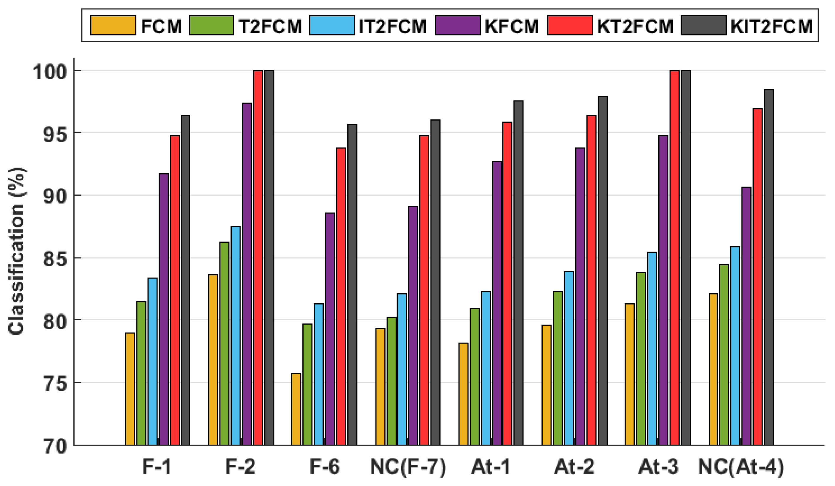
5. Comparative Analysis of Performances

5.1. Comparison with Analogous Condition-Monitoring Algorithms

Below are presented the differences between the proposed method and other fuzzy clustering approaches of related nature. Results for FCM, KFCM, T2FCM, KT2FCM, and IT2FCM algorithms are presented in

Table 6. Confusion matrix for the Tennessee Eastman Process (960 instances in every classification).

FCM
	CON	F-1	F-2	F-6	F-7	At-1	At-2	At-3	At-4	TA(%)
CON	800	0	0	90	70	0	0	0	0	83.33
F-1	0	758	120	0	82	0	0	0	0	78.96
F-2	0	90	803	0	67	0	0	0	0	83.65
F-6	41	45	0	727	57	90	0	0	0	75.73
F-7	22	77	51	0	761	0	0	49	0	79.27
At-1	0	94	0	116	0	750	0	0	0	78.13
At-2	0	0	0	0	0	0	764	0	196	79.58
At-3	38	52	0	0	90	0	0	780	0	81.25
At-4	0	0	0	0	0	0	172	0	788	82.08
AVE										80.22
T2FCM
	CON	F-1	F-2	F-6	F-7	At-1	At-2	At-3	At-4	TA (%)
CON	825	0	0	78	57	0	0	0	0	85.94
F-1	0	782	103	0	75	0	0	0	0	81.46
F-2	0	82	828	0	50	0	0	0	0	86.25
F-6	34	39	0	765	42	80	0	0	0	79.69
F-7	20	75	50	0	770	0	0	45	0	80.21
At-1	0	83	0	100	0	777	0	0	0	80.94
At-2	0	0	0	0	0	0	790	0	170	82.29
At-3	35	45	0	0	76	0	0	804	0	83.75
At-4	0	0	0	0	0	0	150	0	810	84.38
AVE										82.77
IT2FCM
	CON	F-1	F-2	F-6	F-7	At-1	At-2	At-3	At-4	TA (%)
CON	838	0	0	70	52	0	0	0	0	87.29
F-1	0	800	92	0	68	0	0	0	0	83.33
F-2	0	75	840	0	45	0	0	0	0	87.50
F-6	30	35	0	780	40	75	0	0	0	81.25
F-7	17	68	45	0	788	0	0	42	0	82.08
At-1	0	73	0	97	0	790	0	0	0	82.29
At-2	0	0	0	0	0	0	805	0	155	83.85
At-3	32	40	0	0	68	0	0	820	0	85.42
At-4	0	0	0	0	0	0	136	0	824	85.83
AVE										84.32
KFCM
	CON	F-1	F-2	F-6	F-7	At-1	At-2	At-3	At-4	TA(%)
CON	940	0	0	12	8	0	0	0	0	97.92
F-1	0	880	50	0	30	0	0	0	0	91.67
F-2	0	15	935	0	10	0	0	0	0	97.40
F-6	10	16	0	850	34	50	0	0	0	88.54
F-7	14	40	26	0	855	0	0	25	0	89.06
At-1	0	30	0	40	0	890	0	0	0	92.71
At-2	0	0	0	0	0	0	900	0	60	93.75
At-3	10	15	0	0	25	0	0	910	0	94.79
At-4	0	0	0	0	0	0	90	0	870	90.63
AVE										92.94
KT2FCM
	CON	F-1	F-2	F-6	F-7	At-1	At-2	At-3	At-4	TA(%)
CON	960	0	0	0	0	0	0	0	0	100
F-1	0	910	30	0	20	0	0	0	0	94.79
F-2	0	0	960	0	0	0	0	0	0	100
F-6	5	13	0	900	10	32	0	0	0	93.75
F-7	4	24	12	0	910	0	0	10	0	94.79
At-1	0	17	0	23	0	920	0	0	0	95.83
At-2	0	0	0	0	0	0	925	0	35	96.35
At-3	0	0	0	0	0	0	0	960	0	100
At-4	0	0	0	0	0	0	30	0	930	96.88
AVE										96.93
KIT2FCM
	CON	F-1	F-2	F-6	F-7	At-1	At-2	At-3	At-4	TA(%)
CON	960	0	0	0	0	0	0	0	0	100
F-1	0	925	23	0	12	0	0	0	0	96.35
F-2	0	0	960	0	0	0	0	0	0	100
F-6	3	9	0	918	5	25	0	0	0	95.63
F-7	3	18	10	0	922	0	0	7	0	96.04
At-1	0	8	0	16	0	936	0	0	0	97.50
At-2	0	0	0	0	0	0	940	0	20	97.92
At-3	0	0	0	0	0	0	0	960	0	100
At-4	0	0	0	0	0	0	15	0	945	98.44
AVE										97.99

. It is important to note that Fault 7 and Attack 4 are considered New Events for the KIT2FCM algorithm.

Figure 13 visually represents the classification results for different operating states (CON, Faults, and Attacks) in the TE process. In this figure, you can clearly see the excellent outcomes reached by the KIT2FCM algorithm. For all the faults and cyberattacks considered, it achieves classification results above 95%. Furthermore, its ability to identify new events is validated by achieving satisfactory classification results for the fault F-7 and the attack At-4, with 96.04% and 98.44%, respectively.

• Statistical Tests

Statistical tests, as outlined in [39], were used to evaluate whether the obtained results differ significantly. The Friedman test was first applied to detect notable variations among algorithms. If significance was found, Wilcoxon’s test was followed to compare pairs and determine the best performer.

• Friedman Test

The number of algorithms executed was six (k = 6) on 10 distinct sets of data (N = 10). F_F = 340 was selected as the Friedman statistical value, following an F-distribution with df₁ = 5 and df₂ = 45, such that k − 1 = 5 and (k − 1) × (N − 1) = 45. According to the F-distribution table, the critical value for F(5,45) at α = 0.05 is 2.449. Since the calculated F-statistic is less than this critical value (F(5,45) < F_crit), the null hypothesis is rejected, which also signals important dissimilarities between the obtained performances.

• Wilcoxon Test

The outcomes of this test are showcased in

Table 7. Results of the Wilcoxon Test.

	O vs. P	O vs. Q	O vs. R	O vs. S	O vs. W	P vs. Q	P vs. R	P vs. S	P vs. W	Q vs. R	Q vs. S	Q vs. W	R vs. S	R vs. W	S vs. W
$\sum R^{+}$	0	0	0	0	0	5	0	0	0	0	0	0	0	0	5
$\sum R^{-}$	55	55	55	55	55	50	55	55	55	55	55	55	55	55	50
T	0	0	0	0	0	5	0	0	0	0	0	0	0	0	5
$T_{\alpha =0.05}$	8	8	8	8	8	8	8	8	8	8	8	8	8	8	8
Winner	2	3	4	5	6	3	4	5	6	4	5	6	5	6	6

(O: FCM, P: T2FCM, Q: IT2FCM, R: KFCM, S: KT2FCM, W: KIT2FCM). The initial two rows present values for R⁺ (summatory of the positive ranks) and R⁻ (sum of the negative ranks). The subsequent rows present the statistical value T, along with the crucial value of T for a significance level of α = 0.05. Lastly, the prevailing algorithm for every comparison is presented.

Table 8. Results of the comparative analysis of performances.

Algorithm	Number of Wins	Rank
O	0	6
P	1	5
Q	2	4
R	3	3
S	4	2
W	5	1

provides a summary of the number of wins for each algorithm.

5.2. With Recent Algorithms

This section presents the results of a comparison of the proposed scheme with modern fault detection and location methods, using Fault 3, Fault 9, and Fault 15 of the TEP (see

Table 9. Faults that were analyzed in the TEP.

Fault	Process Variable	Type
Fault 3 (F-3)	D feed temperature (stream 2) Reactor cooling water inlet	step
Fault 9 (F-9)	D feed temperature (stream 2)	random
Fault 15 (F-15)	Condenser cooling water valve	sticking

).

Based on the conducted research, Fault 3, Fault 9, and Fault 15 exhibit minor discrepancies compared to the CON of the process, rendering them very intricate to accurately classify. A depiction of the confusion matrix obtained by using the KIT2FCM algorithm for these faults and the CON is presented in

Table 10. Confusion matrix: KIT2FCM (CON: 960, Fault 3: 960, Fault 9: 960, Fault 15: 960).

	CON	F-3	F-9	F-15	TA (%)
CON	915	13	11	21	95.31
F-3	39	891	20	10	92.81
F-9	50	31	854	25	88.96
F-15	74	32	35	819	85.31
AVE					90.60

.

Other methods used to compare were presented in [40,41,42,43]. They are based on the following types of deep learning algorithms: Deep Belief Network (DBN), Deep Convolutional Neural Network (DCNN), Bidirectional Gated Recurrent Unit (BiGRU), Process Topology Convolutional Network (PTCN).

Table 11. Results of the comparison (values in bold indicate the best performance).

Fault	DBN(%)	DCNN(%)	BiGRU(%)	PTCN(%)	KIT2FCM (%)
F-3	95.00	91.70	93.50	88.04	92.81
F-9	57.00	58.40	80.70	66.01	88.96
F-15	0.00	28.00	54.10	0.35	85.31
AVE	50.66	59.36	76.10	51.46	89.03

presents the results obtained. These results reaffirm the reliability and robust performance of the proposed strategy.

6. Conclusions

A strategy for cybersecurity and health management with continuous learning of chemical processes utilizing computational intelligence tools has been presented, constituting a significant scientific contribution in this paper. This strategy seamlessly incorporates the detection and categorization of faults and cyberattacks, yielding good results in the presence of noisy data, which further underscores its importance. Type-2 fuzzy sets are employed to address challenges posed by T1 fuzzy sets in effectively modeling the uncertainty inherent in the data obtained from within industrial processes, stemming from noise and external perturbations.

In the proposed approach, the offline training step is vital. The Interval Type-2 FCM algorithm is initially used as a classifying tool to group known classes (CON and COA) while handling noise and external perturbations. A Knowledge Base is then employed to identify the specific Abnormal Operation Condition (COA: Fault/Attack) that influences the plant, which is a key strength of this strategy. Additionally, a kernel-based version of IT2FCM (KIT2FCM) is introduced to improve class separation and minimize classification errors. In this regard, the results achieved demonstrate the ability of the proposed system based on T2FS + FIS to perform training robustly. The KIT2FCM algorithm, together with the obtained knowledge base (Table 4), allows the monitoring system to be successfully trained based on the faults and cyberattacks that have affected the TE process.

During the online recognition phase, the proposed method can detect new events, such as cyberattacks or faults. Once these events are identified and characterized, new patterns are added to the historical database, and further training is conducted. The performance achieved in this stage by the condition-monitoring system is evident in Table 6 and Figure 3, where the KIT2FCM algorithm achieves the best results. The ability to identify new events is successfully validated with the classification of the fault F-7 and the attack At-4.

Furthermore, a comprehensive comparison was made with several algorithms presented in the scientific literature. In all instances, the suggested method demonstrates superior performance, even when evaluated in the classification of challenging faults (3, 9, and 15) in the TE process. These faults are renowned for their difficulty in accurate classification, highlighting the robustness and effectiveness of the proposed strategy.

References

1. Macas, M.; Wu, C.; Fuertes, W. A survey on deep learning for cybersecurity: Progress, challenges, and opportunities. Comput. Netw. 2022, 212, 109032. [Google Scholar] [CrossRef]
2. Bashendy, M.; Tantawy, A.; Erradi, A. Intrusion response systems for cyber-physical systems: A comprehensive survey. Comput. Secur. 2023, 124, 102984. [Google Scholar] [CrossRef]
3. Alanazi, M.; Mahmood, A.; Morshed, M.J. SCADA vulnerabilities and attacks: A review of the state of the art and open issues. Comput. Secur. 2023, 125, 103028. [Google Scholar] [CrossRef]
4. Alladi, T.; Chamola, V.; Zeadally, S. Industrial Control Systems: Cyberattack trends and countermeasur. Comput. Commun. 2020, 155, 1–8. [Google Scholar] [CrossRef]
5. Azzam, M.; Pasquale, L.; Provan, G.; Nuseibeh, B. Forensic readiness of industrial control systems under stealthy attacks. Comput. Secur. 2023, 125, 103010. [Google Scholar] [CrossRef]
6. Parker, S.; Wu, Z.; Christofides, P.D. Cybersecurity in process control, operations, and supply chain. Comput. Chem. Eng. 2023, 171, 108169. [Google Scholar] [CrossRef]
7. Fernandes, M.; Corchado, J.M.; Marreiros, G. Machine learning techniques applied to mechanical fault diagnosis and fault prognosis in the context of real industrial manufacturing use-cases: A systematic literature review. Appl. Intell. 2022, 52, 14246–14280. [Google Scholar] [CrossRef]
8. Li, W.; Huang, R.; Li, J.; Liao, Y.; Chen, Z.; He, G.; Yan, R.; Gryllias, K. A perspective survey on deep transfer learning for fault diagnosis in industrial scenarios: Theories, applications and challenges. Mech. Syst. Signal Process. 2022, 167, 108487. [Google Scholar] [CrossRef]
9. Lv, H.; Chen, J.; Pan, T.; Zhang, T.; Feng, Y.; Liu, S. Attention mechanism in intelligent fault diagnosis of machinery: A review of technique and application. Measurement 2022, 199, 111594. [Google Scholar] [CrossRef]
10. Mu, B.; Scott, J.K. Set-based fault diagnosis for uncertain nonlinear systems. Comput. Chem. Eng. 2024, 180, 108479. [Google Scholar] [CrossRef]
11. Quian, J.; Song, Z.; Yao, Y.; Zhu, Z.; Zhang, X. A review on autoencoder based representation learning for fault detection and diagnosis in industrial processes. Chemom. Intell. Lab. Syst. 2022, 231, 104711. [Google Scholar] [CrossRef]
12. Vidal-Puig, S.; Vitale, R.; Ferrer, A. Data-driven supervised fault diagnosis methods based on latent variable models: A comparative study. Chemom. Intell. Lab. Syst. 2019, 187, 41–52. [Google Scholar] [CrossRef]
13. Doing, D.; Han, Q.L.; Xiang, Y.; Zhang, X.M. New Features for Fault Diagnosis by Supervised Classification. IEEE Trans. Instrum. Meas. 2021, 70, 1–15. [Google Scholar]
14. Zang, P.; Wen, G.; Dong, S.; Lin, H.; Huang, X.; Tian, X.; Chen, X. A novel multiscale lightweight fault diagnosis model based on the idea of adversarial learning. Neurocomputing 2018, 275, 1674–1683. [Google Scholar]
15. Camps-Echevarría, L.; Llanes Santiago, O.; Campos Velho, H.F.d.; Silva Neto, A.J.d. Fault Diagnosis Inverse Problems. In Fault Diagnosis Inverse Problems: Solution with Metaheuristics; Springer: Cham, Switzerland, 2019. [Google Scholar]
16. Kravchik, M.; Demetrio, L.; Biggio, L.; Shabtai, A. Practical Evaluation of Poisoning Attacks on Online Anomaly Detectors in Industrial Control System. Comput. Secur. 2022, 122, 102901. [Google Scholar] [CrossRef]
17. Zhou, J.; Zhu, Y. Fault isolation based on transfer-function models using an MPC algorithm. Comput. Chem. Eng. 2022, 159, 107668. [Google Scholar] [CrossRef]
18. Prieto-Moreno, A.; Llanes-Santiago, O.; García-Moreno, E. Principal components selection for dimensionality reduction using discriminant information applied to fault diagnosis. J. Process Control 2015, 33, 4–24. [Google Scholar] [CrossRef]
19. Lundgren, A.; Jung, D. Data-driven fault diagnosis analysis and open-set classification of time-series data. Control Eng. Pract. 2022, 121, 105006. [Google Scholar] [CrossRef]
20. Taqvi, S.A.A.; Zabiri, H.; Tufa, L.D.; Uddinn, F.; Fatima, S.A.; Maulud, A.S. A review on data-driven learning approaches for fault detection and diagnosis in chemical process. ChemBioEng Rev. 2021, 8, 39–259. [Google Scholar] [CrossRef]
21. Kumar, N.; Mohan Mishra, V.; Kumar, A. Smart grid and nuclear power plant security by integrating cryptographic hardware chip. Nucl. Eng. Technol. 2021, 53, 3327–3334. [Google Scholar] [CrossRef]
22. Hadroug, N.; Hafaifa, A.; Alili, B.; Iratni, A.; Chen, X. Fuzzy Diagnostic Strategy Implementation for Gas Turbine Vibrations Faults Detection: Towards a Characterization of Symptom Fault Correlations. J. Vib. Eng. Technol. 2022, 10, 225–251. [Google Scholar] [CrossRef]
23. Chi, Y.; Dong, Y.; Wang, Z.Y.; Yu, F.R.; Leung, V.C.M. Knowledge-Based Fault Diagnosis in Industrial Internet of Things: A Survey. IEEE Internet Things J. 2022, 9, 12886–12900. [Google Scholar] [CrossRef]
24. Rodríguez-Ramos, A.; Bernal-de-Lázaro, J.M.; Cruz-Corona, C.; Silva Neto, A.J.; Llanes-Santiago, O. An approach to robust condition monitoring in industrial processes using pythagorean memberships grades. Ann. Braz. Acad. Sci. 2022, 94, e20200662. [Google Scholar] [CrossRef] [PubMed]
25. Zhou, K.; Tang, J. Harnessing fuzzy neural network for gear fault diagnosis with limited data labels. Int. J. Adv. Manuf. Tech. 2021, 115, 1005–1019. [Google Scholar] [CrossRef]
26. Fan, Y.; Ma, T.; Xiao, F. An improved approach to generate generalized basic probability assignment based on fuzzy sets in the open world and its application in multi-source information fusion. Appl. Intell. 2021, 51, 3718–3735. [Google Scholar] [CrossRef]
27. Pan, H.; Xu, H.; Zheng, J.; Su, J.; Tong, J. Multi-class fuzzy support matrix machine for classification in roller bearing fault diagnosis. Adv. Eng. Inform. 2021, 51, 101445. [Google Scholar] [CrossRef]
28. Yang, X.; Yu, F.; Pedrycz, W. Typical Characteristic-Based Type-2 Fuzzy C-Means Algorithm. IEEE Trans. Fuzzy Syst. 2021, 29, 1173–1187. [Google Scholar] [CrossRef]
29. Yin, Y.; Sheng, Y.; Qin, J. Interval type-2 fuzzy C-means forecasting model for fuzzy time series. Appl. Soft Comput. 2022, 129, 109574. [Google Scholar] [CrossRef]
30. Li, Q.; Chen, B.; Chen, Q.; Li, X.; Qin, Z.; Chu, F. HSE: A plug-and-play module for unified fault diagnosis foundation models. Inf. Fusion 2025, 123, 103277. [Google Scholar] [CrossRef]
31. Amin, T.; Halim, S.Z.; Pistikopoulos, S. A holistic framework for process safety and security analysis. Comput. Chem. Eng. 2022, 165, 107693. [Google Scholar] [CrossRef]
32. Syfert, M.; Ordys, A.; Koscielny, J.M.; Wnuk, P.; Mozaryn, J.; Kukielka, K. Integrated approach to diagnostics of failures and cyber-attacks in industrial control systems. Energies 2022, 15, 6212. [Google Scholar] [CrossRef]
33. Dai, S.; Zha, L.; Liu, J.; Xie, X.; Tian, E. Fault detection filter design for networked systems with cyber attacks. Appl. Math. Comput. 2022, 412, 126593. [Google Scholar] [CrossRef]
34. Müller, N.; Bao, K.; Matthes, J.; Heussen, K. Cyphers: A cyberphysical event reasoning system providing real-time situational awareness for attack and fault response. Comput. Ind. 2023, 151, 103982. [Google Scholar] [CrossRef]
35. Ester, M.; Kriegel, H.; Sander, J.; Xu, X. A density-based algorithm for discovering clusters in large spatial databases with noise. In 2nd ACM SIGKDD; AAAI Press: Washington, DC, USA, 1996; pp. 226–231. [Google Scholar]
36. Bathelt, A.; Ricker, N.L.; Jelali, M. Revision of the Tennessee Eastman Process model. IFAC Pap. OnLine 2015, 48, 309–314. [Google Scholar] [CrossRef]
37. Melo, A.; Câmara, M.M.; Clavijo, N.; Pinto, J. Open benchmarks for assessment of process monitoring and fault diagnosis techniques: A review and critical analysis. Comput. Chem. Eng. 2022, 165, 107964. [Google Scholar] [CrossRef]
38. Rodríguez-Ramos, A.; Ortiz, F.J.; Llanes-Santiago, O. A proposal of Robust Condition Monitoring Scheme for Industrial Systems. Comput. Sist. 2023, 27, 223–235. [Google Scholar] [CrossRef]
39. García, S.; Herrera, F. An extension on statistical comparisons of classifiers over multiple datasets for all pairwise comparisons. J. Mach. Learn. Res. 2008, 9, 2677–2694. [Google Scholar]
40. Zhang, Z.; Zhao, J. A deep belief network based fault diagnosis model for complex chemical processes. Comput. Chem. Eng. 2017, 107, 395–407. [Google Scholar] [CrossRef]
41. Wu, H.; Zhao, J. Deep convolutional neural network model based chemical process fault diagnosis. Comput. Chem. Eng. 2018, 115, 185–197. [Google Scholar] [CrossRef]
42. Zhang, S.; Bi, K.; Qiu, T. Bidirectional recurrent neural network based chemical process fault diagnosis. Ind. Eng. Chem.Res. 2020, 59, 824–834. [Google Scholar] [CrossRef]
43. Wu, D.; Zhao, J. Process topology convolutional network model for chemical process fault diagnosis. Process Saf. Environ. Prot. 2021, 150, 93–109. [Google Scholar] [CrossRef]
Figure 1. Result of applying the KFCM algorithm.
Actuators 14 00329 g001
Figure 2. Triangular primary and secondary membership functions.
Actuators 14 00329 g002
Figure 3. Two instances of Type 2 TMF: (a) ambiguity in standard deviation and (b) ambiguity in mean.
Actuators 14 00329 g003
Figure 4. Scheme for the classification of condition monitoring, with faults and cyberattacks.
Actuators 14 00329 g004
Figure 5. Functions defining the membership of symptom variables in the process evaluation.
Actuators 14 00329 g005
Figure 6. Methodology for obtaining the Knowledge Base.
Actuators 14 00329 g006
Figure 7. Procedure performed at the training phase.
Actuators 14 00329 g007
Figure 8. Detailed scheme for the online detection of new events.
Actuators 14 00329 g008
Figure 9. Diagram of the TEP.
Actuators 14 00329 g009
Figure 10. Fault 6 occurrence, Tennessee Eastman process.
Actuators 14 00329 g010
Figure 11. Occurrence of Attack 2 in the Tennessee Eastman process.
Actuators 14 00329 g011
Figure 12. Classification of the scenarios for the Tennessee Eastman Process.
Actuators 14 00329 g012
Figure 13. Faults and attacks classification (in %) for the Tennessee Eastman Process.
Actuators 14 00329 g013