Adaptive Linear Active Disturbance Rejection Cooperative Control of Multi-Point Hybrid Suspension System

Abstract

The hybrid maglev train exhibits advantages such as a large suspension gap, high load-to-weight ratio, and low suspension energy consumption. However, challenges, including unmodeled uncertainties and multi-point coupling interference in the suspension system, may degrade control performance. To enhance the global anti-interference capability of the multi-point hybrid suspension system, an adaptive linear active disturbance rejection cooperative control (ALADRCC) method is proposed. First, dynamic models of single-point and multi-point hybrid suspension systems are established, and coupling relationships among multiple suspension points are analyzed. Second, an adaptive linear extended state observer (ALESO) is designed to improve dynamic response performance and noise suppression capability. Subsequently, a coupling cooperative compensator (CCC) is designed and integrated into the linear error feedback control law of adaptive linear active disturbance rejection control (ALADRC), enabling cross-coupling compensation between the suspension gap and its variation rate to enhance multi-point synchronization. Then, the simulation models are constructed on MATLAB/Simulink to validate the effectiveness of ALESO and CCC. Finally, a multi-point hybrid suspension experimental platform is built. Comparative experiments with PID and conventional LADRC demonstrate that the proposed ALADRC achieves faster response speed and effective system noise suppression. Additional comparisons with PID and ALADRC confirm that ALADRCC significantly reduces synchronization errors between adjacent suspension points, exhibiting superior global anti-interference performance.

1. Introduction

Magnetic suspension technology is characterized by fast response, high precision, clean, and non-polluting, and is widely used in magnetic levitation transportation, industrial manufacturing, medical equipment, and aerospace, among others. At present, electromagnetic suspension technology is more widely used, but pure electromagnetic levitation devices have problems with electromagnet heating and high levitation energy consumption during continuous operation [1]. With the breakthrough in the performance of rare earth permanent magnet materials, the application of permanent magnet–electromagnetic hybrid levitation technology to magnetic levitation trains has significant technical advantages. Through the permanent magnet to provide part of the suspension force, the electromagnetic field dynamically adjusts the levitation force, which can significantly reduce the levitation energy consumption, increase the suspension gap, and improve the load carrying specific gravity [2]. However, the introduction of permanent magnets leads to the enhancement in the nonlinearity of the suspension system, accompanied by magnetic field coupling and other uncertainties, which increases the control difficulty of the hybrid suspension system [3].

The permanent magnet–electromagnetic hybrid suspension system consists of multiple sets of electromagnets and permanent magnets, which is a typical multiple-input–multiple-output nonlinear coupling system. For the control study of a multi-point hybrid suspension system, the traditional method is to decouple the multi-point hybrid suspension system into a single point for independent control and then design the corresponding control strategy according to the performance index of the single-point hybrid suspension system. Such as PID control [4], sliding mode control [5], model predictive control [6], etc. Although the above control strategy meets the control requirements to a certain extent, there are still some shortcomings. For instance, the PID control is based on error feedback to eliminate the error, which makes it difficult to take into account the control requirements of fast response and overshoot suppression in complex systems, and the adaptive ability of nonlinear and time-varying systems is poor. Additionally, the sliding-mode control is prone to cause high-frequency oscillations, which affects the life of the actuator and the performance of the system; the order of the model predictive controller is high, and the real-time control is not suitable for the real-time control of the system. The order of the model predictive controller is high, and the real-time rolling optimization solution makes the computation large, and the performance seriously depends on the accuracy of the system model. Linear active disturbance rejection control (LADRC), as an improvement and refinement of traditional PID control, has a strong adaptive ability to system parameter changes and can effectively suppress uncertainties and external disturbances, which is especially suitable for the field of suspension control [7,8,9]. Aiming at the parameter tuning problem of LADRC, the literature [10] designed the LADRC control algorithm based on the model of the permanent magnet electromagnetic hybrid suspension platform and introduced the fuzzy control into the LADRC state error feedback control theory to realize the parameter self-tuning and improve the adaptability and robustness of the system. Although the self-resistant structure is improved to simplify the adjustment of the key parameters, the expansion of the state observation bandwidth of the observer does not have good self-tuning capability.

In summary, many scholars have proposed and validated their own improvement methods for single-point hybrid suspension control systems from different perspectives. The control performance of a single suspension point needs to be considered not only during the operation of a magnetic levitation train but also during the coupling perturbation between the suspension points for the impact on the overall control performance. Cooperative control has become a solution to the coupling perturbation problem in the suspension system. The cooperative control strategy will be a single suspension point control strategy associated with each other to achieve synchronous control of multiple suspension points. Cooperative control has been widely used in other fields [11,12,13]. Literature [14] proposes a decentralized cooperative control framework for the integration of active front steering and active suspension systems by applying a multi-constraint distributed model predictive control approach, which effectively improves the lateral stability, ride comfort, and lateral sway safety of the vehicle during path tracking. Literature [15] constructs a semi-vehicle dynamics system that integrates torque vectoring and an active suspension system to improve the vehicle’s longitudinal and vertical motion control performance, considering safety, energy efficiency, and comfort requirements. In the field of magnetic levitation, there are also many scholars who use cooperative control to control multiple suspension points. Literature [16] proposed a dynamic synchronization control strategy based on the steel plate dynamics model for the limitation of single electromagnet levitation control, which effectively coordinates the role of multi-electromagnets and improves the suspension stability and control accuracy through the double cross-coupling control and coupling compensation of air gap and velocity. Literature [17] proposed a cross-coupling control strategy, which overcomes the inadequacy of previous control algorithms based on the assumption of complete decoupling by compensating the output error of the multi-point levitation system and exhibits high control accuracy and strong robustness. Literature [18] proposed a LESO-backstepping control method based on the dual coupling of the air gap and the velocity for the suspension frame of a magnetically levitated vehicle by means of a virtual controller and extended state observer to compensate for the disturbance and improve the synchronization performance of each suspension point. Literature [19] proposed a super-torsion sliding mode control method based on adaptive fuzzy compensation for maglev trains affected by coupling effect, track unevenness, and time-varying disturbances to achieve accurate suspension and effectively suppress system jitter under a nonlinear model. Literature [20] designed a hyper-localized sliding mode controller to reduce the model dependence and fused adjacent coupling control to effectively reduce the tracking error and synchronization error of each suspension point to enhance the anti-jamming ability of the multi-point magnetic levitation system. The cooperative control theory has been widely used in multi-point suspension systems, but the current research mainly focuses on the normally-conductive magnetic levitation system, while the research on multi-point hybrid suspension systems is still relatively limited.

In this paper, a multi-point hybrid suspension system is investigated with the core objectives of improving the synchronization performance of the suspension system and enhancing the comprehensive system immunity. The specific work and contributions are as follows:

(1)

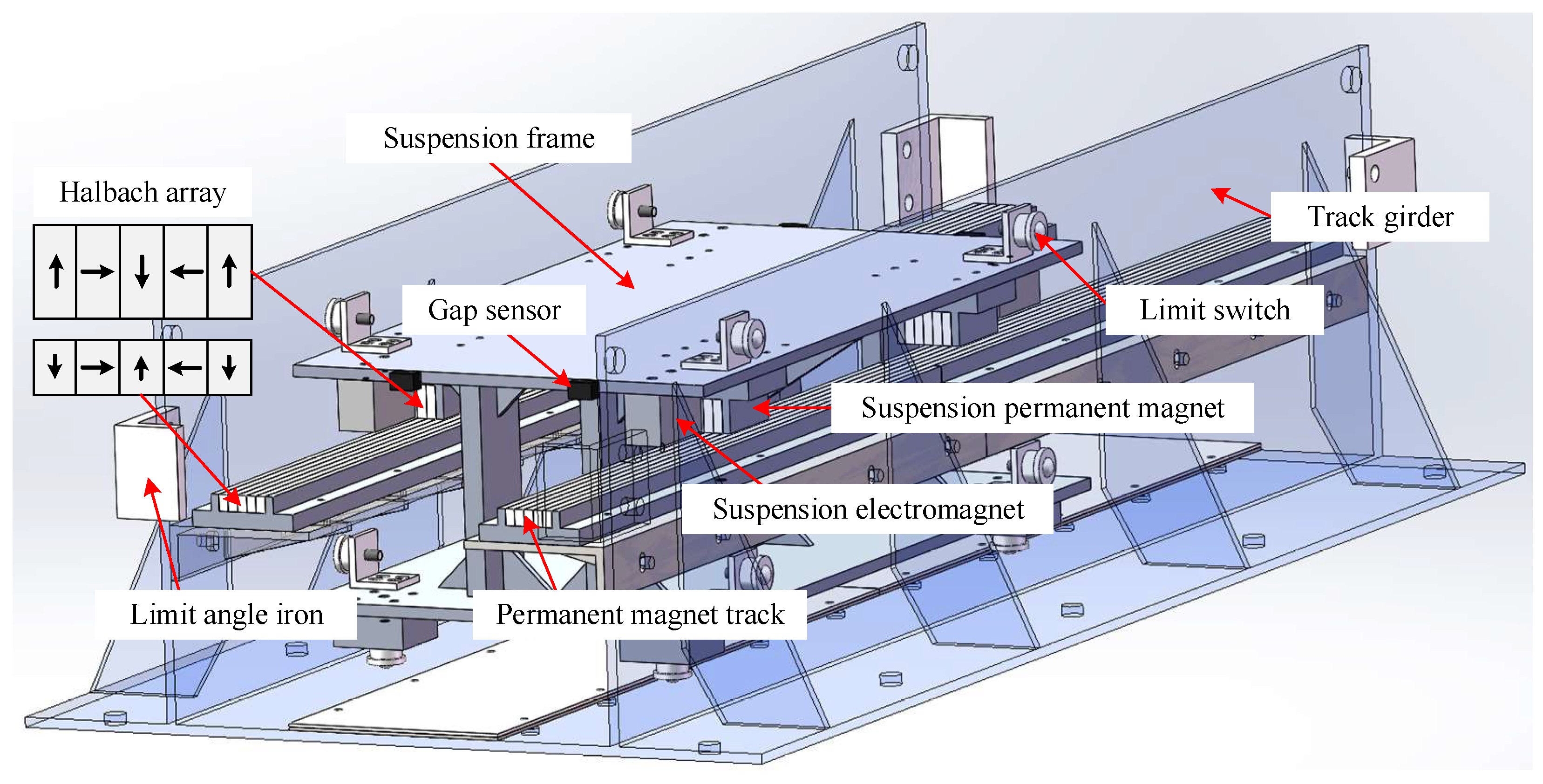
The structure and working principle of the hybrid suspension system are analyzed, the single-point and multi-point hybrid suspension system models are established, respectively, and the coupling relationship between multiple suspension points is deduced.

(2)

Aiming at the uncertainties caused by the permanent magnet–electromagnetic combination, such as the enhancement in system nonlinearity and the increase in magnetic field coupling, ALESO is designed to simultaneously improve the dynamic response performance and noise rejection of the hybrid suspension system.

(3)

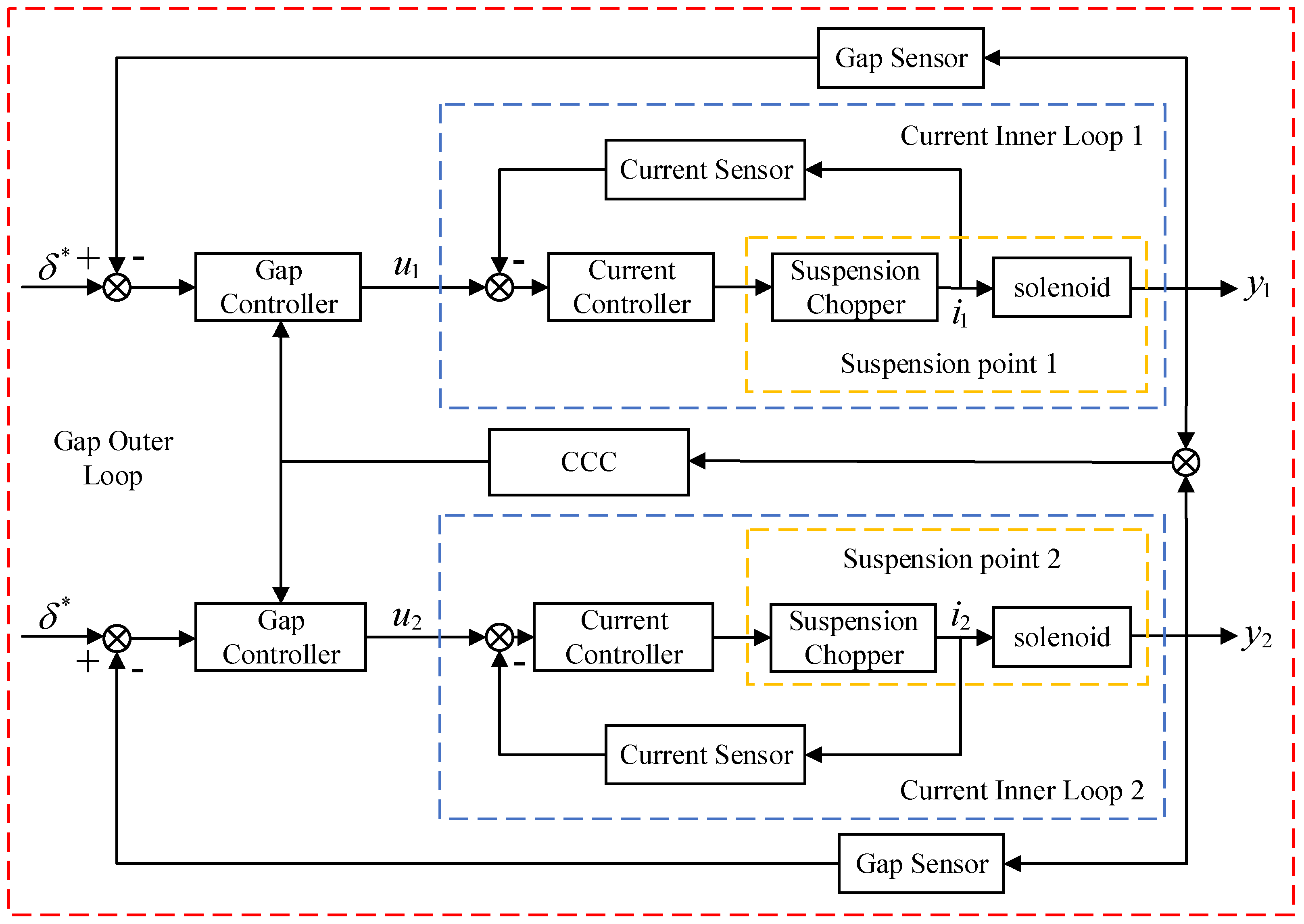
Aiming at the lack of synchronization coordination mechanism in independent control mode, the CCC is designed and integrated into the linear error feedback control law of the ALADRC algorithm to realize the cross-coupling of the suspension gap and its rate of change to enhance the synchronous coordination of the multi-point suspension system.

(4)

A multi-point permanent magnet electromagnetic hybrid suspension experimental platform is built to carry out single-point suspension, unilateral suspension, and four-point suspension experiments to verify the effectiveness of the control algorithm designed in this paper.

The remainder of the paper is organized as follows. Section 2 models the multi-point hybrid suspension system. Section 3 carries out the controller design and designs the gap outer loop-current inner loop series dual closed-loop control architecture, where the current inner loop uses a PI controller to speed up the system response, and the gap outer loop uses the ALADRCC to ensure that the system maintains stable suspension. Simulation experiments are conducted in Section 4 to verify the effectiveness of ALESO and CCC. Section 5 builds a multi-point hybrid suspension experimental platform for practical algorithm comparison and validation and analyzes the experimental results. The summary and conclusions are presented in Section 6.

2. Multi-Point Hybrid Suspension System Modeling

2.1. Structure and Principle Analysis of Hybrid Suspension System

The R&D team of this research group innovatively proposes a multi-point hybrid suspension structure, as shown in Figure 1. The structure relies on the Halbach array, composed of suspension permanent magnets and permanent magnet tracks, to provide the main suspension force and enhance the controllability, stability, and robustness of the suspension system through an electromagnetic damping structure. The suspension frame is embedded in the track girder, and the limit wheel ensures the vertical centering of the Halbach array, prevents the suspension frame from moving from side to side during levitation, and maximizes the levitation force provided by the permanent magnets. Suspension electromagnets and suspension permanent magnets are installed in parallel in the suspension frame, forming four hybrid suspension units. When the system is energized, the hybrid magnetic field generates a repulsive force that overcomes gravity to stabilize the suspension frame in the track girder. This suspension structure effectively avoids the problem of “suction death” of the rail, but it also increases the complexity of the system control and puts forward higher requirements for precise control.

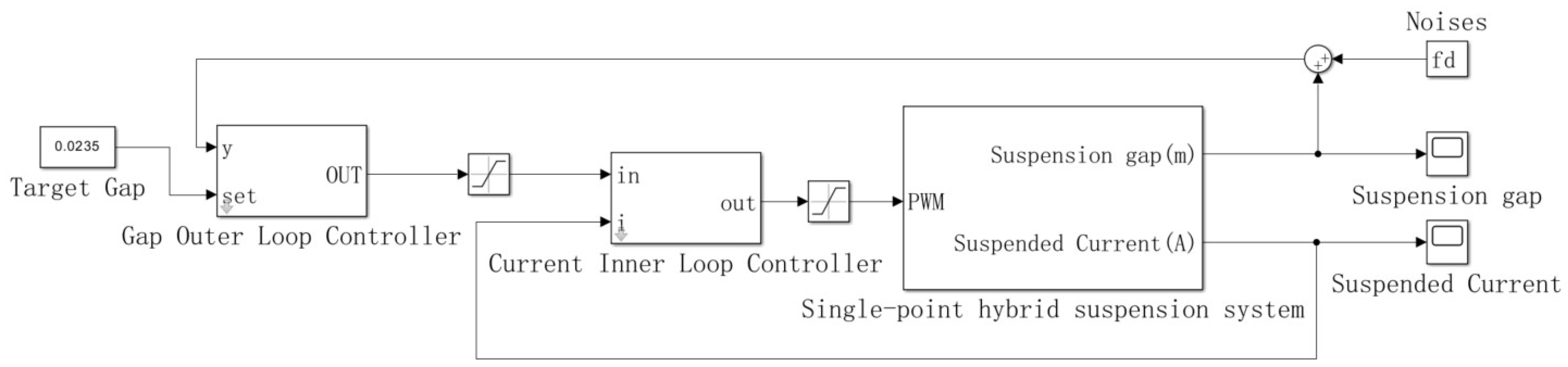
2.2. Single-Point Hybrid Suspension System Model

Each suspension point of the multi-point hybrid suspension system is equipped with an independent suspension control loop, and its structure and function are basically the same. An in-depth understanding of the characteristics of the single-point hybrid suspension system is an important prerequisite for the study and application of magnetic levitation technology, and it is also the basis for exploring the multi-point hybrid suspension system. Figure 2 shows the dynamics model of the single-point hybrid suspension system. The system consists of the upper and lower opposing Halbach permanent magnet arrays and suspension electromagnets, which together provide the required levitation force to support the levitation platform.

Where $\delta (t)$ is the suspension gap, $m$ is the mass of the suspension frame acting on the suspension point, $g$ is the gravitational acceleration, $F_p(\delta )$ is the permanent magnetic levitation force generated by the Halbach permanent magnet array, $F_e(i,\delta )$ is the electromagnetic levitation force generated by the levitation electromagnet, $f_d$ is the external perturbation, $u(t)$ is the voltage at the ends of the electromagnetic coil, and $i(t)$ is the electromagnetic coil current.

According to the theory of electromagnetism, the electromagnetic suspension force of the system can be expressed as follows:

$$F_e(i,\delta )={\displaystyle \frac{{\mu }_0{N}^{2}S}{4}}{\left[{\displaystyle \frac{i\left(t\right)}{\delta (t)}}\right]}^2$$

(1)

where ${\mu }_0$ is the air permeability; $N$ is the number of coil turns; and $S$ is the pole area.

Due to the uncontrollable magnetic force generated by the permanent magnet, the magnetic force decays as the gap with the permanent magnet increases, and there is a range fluctuation in the magnetic force at static. In this paper, the permanent magnetic suspension force of the system obtained by finite element simulation analysis and data fitting can be expressed as follows:

$$F_p(\delta )=k{e}^{b\delta (t)}+\mathrm{c}$$

(2)

where $k$ = 1621.27, $b$ = −152.84, $\mathrm{c}$ = 128.36, $e$ = 2.71828.

Let the internal resistance of the coil of the suspension solenoid be $R$, and the voltage equation for the suspension solenoid circuit can be written as follows:

$$u\left(t\right)=Ri\left(t\right)+{\displaystyle \frac{{\mu }_0{N}^{2}S}{2\delta \left(t\right)}}{\displaystyle \frac{di\left(t\right)}{dt}}-{\displaystyle \frac{{\mu }_0{N}^{2}Si\left(t\right)}{2{\left[\delta \left(t\right)\right]}^2}}{\displaystyle \frac{d\delta \left(t\right)}{dt}}$$

(3)

Combined with the kinetic equations, the nonlinear mathematical model of a single-point hybrid suspension system can be represented by the following system of equations:

$$\left\{\begin{array}{l}m{\displaystyle \frac{d^2{\delta }_i\left(t\right)}{d{t}^2}}=F_i\left(i_i,{\delta }_i\right)-mg+f_{di}(t)\\ F_i\left(i_i,{\delta }_i\right)=F_{\mathrm{ei}}\left(i,\delta \right)+F_{pi}(\delta )={\displaystyle \frac{{\mu }_0{N}^{2}S}{4}}{\left[{\displaystyle \frac{i_i\left(t\right)}{{\delta }_i(t)}}\right]}^2+k{e}^{b{\delta }_i(t)}+\mathrm{c}\\ u_i\left(t\right)=R{i}_i\left(t\right)+{\displaystyle \frac{{\mu }_0{N}^{2}S}{2[{\delta }_i(t)]}}{\displaystyle \frac{d{i}_i\left(t\right)}{dt}}-{\displaystyle \frac{{\mu }_0{N}^{2}S{i}_i\left(t\right)}{2{\left[{\delta }_i(t)\right]}^2}}{\displaystyle \frac{d{\delta }_i\left(t\right)}{dt}}\end{array}\right.$$

(4)

Linearizing the above system of nonlinear equations around the equilibrium point $(i_0,{\delta }_0)$ yields a linearized model of the system as follows:

$$\left\{\begin{array}{l}m\Delta \ddot{\delta }=k_{ei}\Delta i+(k_{e\delta }+k_{p\delta })\Delta \delta +f_d\\ \Delta u=R\Delta i+L_0\Delta \dot{i}-k_{ei}\Delta \dot{\delta }\end{array}\right.$$

(5)

where $k_{ei}={\displaystyle \frac{{\mu }_0{N}^{2}S{i}_0}{2{{\delta }_0}^2}}$, $k_{e\delta }=-{\displaystyle \frac{{\mu }_0{N}^{2}S{i_0}^2}{2{{\delta }_0}^3}}$, $kb{e}^{b{\delta }_0}=k_{p\delta }$, $L_0={\displaystyle \frac{{\mu }_0{N}^{2}S}{2{\delta }_0}}$.

By selecting the voltage at both ends of the suspension electromagnet as input, the current, the suspension gap, and its derivative as intermediate variables, and the suspension gap as output, the linearized system equations can be collated to obtain the following state space expression:

$$\left\{\begin{array}{l}\left[\begin{array}{c}\Delta \dot{\delta }\\ \Delta \ddot{\delta }\\ \Delta \dot{i}\end{array}\right]=\left[\begin{array}{ccc}0& 1& 0\\ {\displaystyle \frac{k_{e\delta }+k_{p\delta }}{m}}& 0& {\displaystyle \frac{k_{ei}}{m}}\\ 0& {\displaystyle \frac{k_{ei}}{L_0}}& -{\displaystyle \frac{R}{L_0}}\end{array}\right]\left[\begin{array}{c}\Delta \delta \\ \Delta \dot{\delta }\\ \Delta i\end{array}\right]+\left[\begin{array}{cc}0& 0\\ 0& 1\\ {\displaystyle \frac{1}{L_0}}& 0\end{array}\right]\left[\begin{array}{c}\Delta u(t)\\ \Delta f_d(t)\end{array}\right]\\ y=\left[\begin{array}{ccc}1& 0& 0\end{array}\right]\left[\begin{array}{c}\Delta \delta \\ \Delta \dot{\delta }\\ \Delta i\end{array}\right]\end{array}\right.$$

(6)

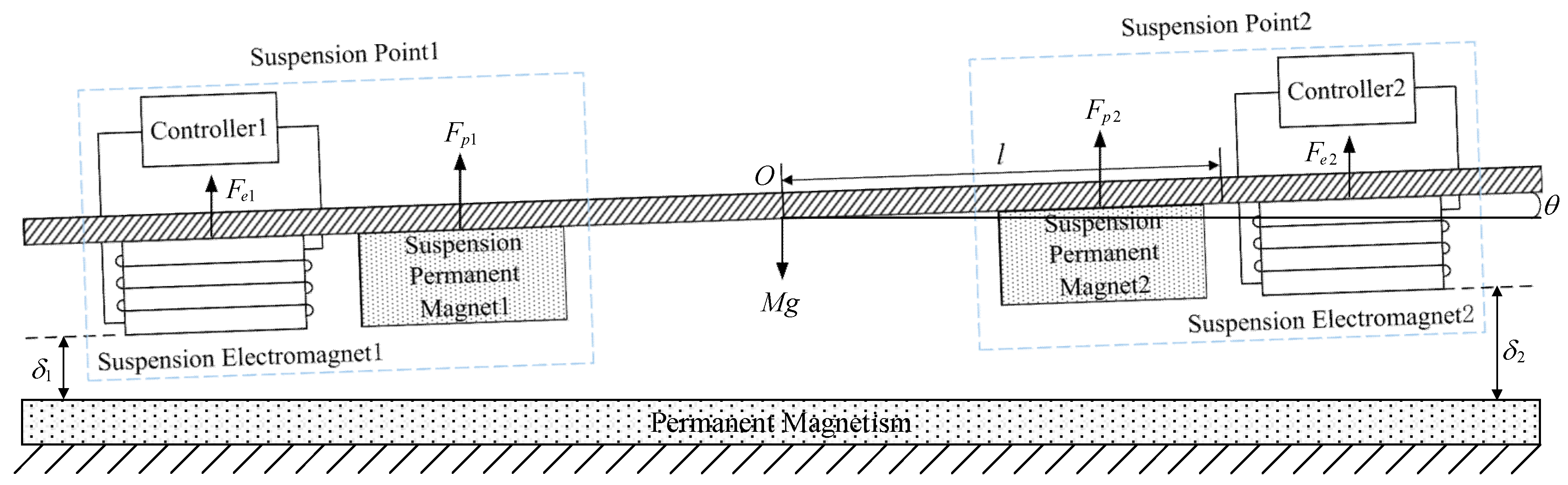
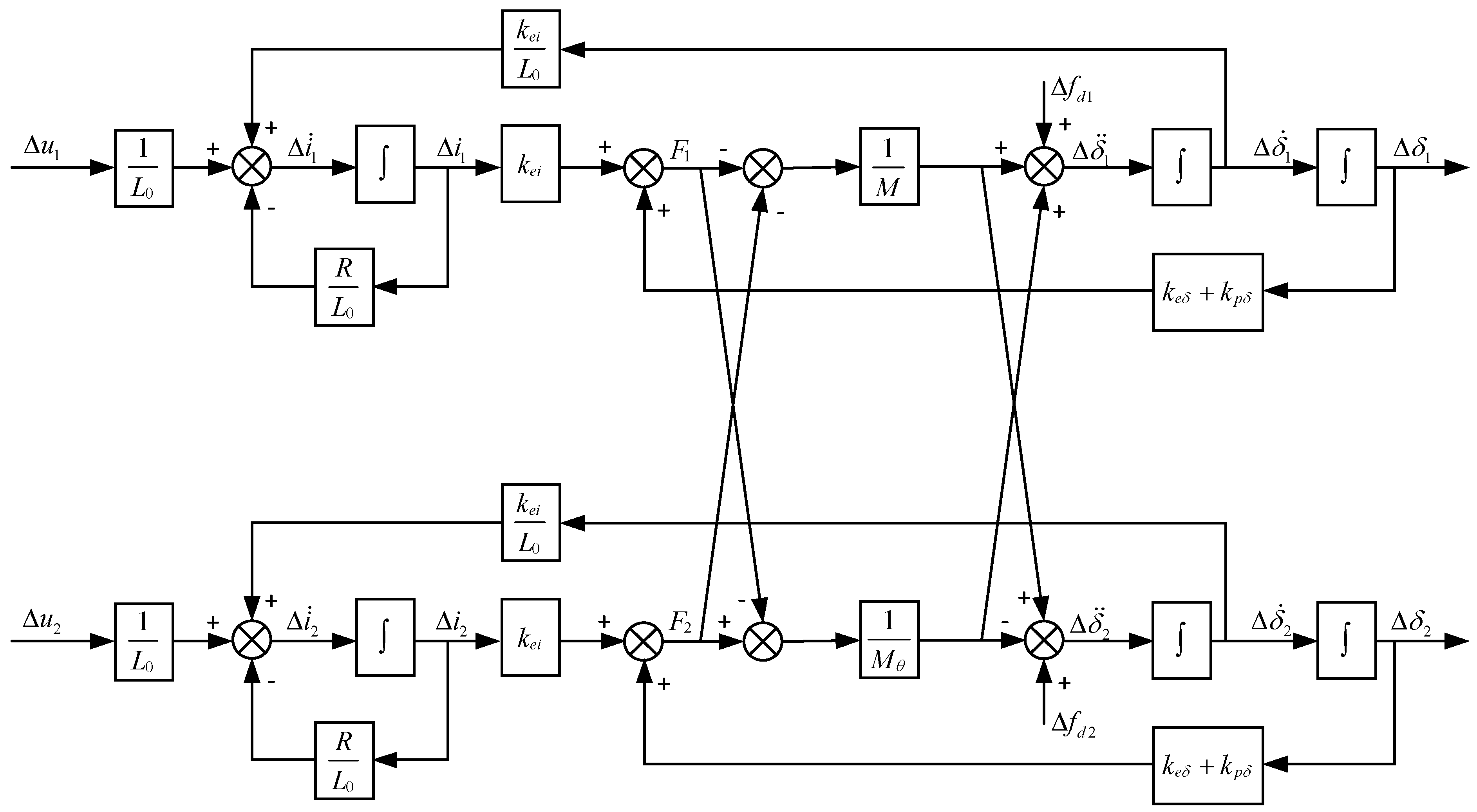
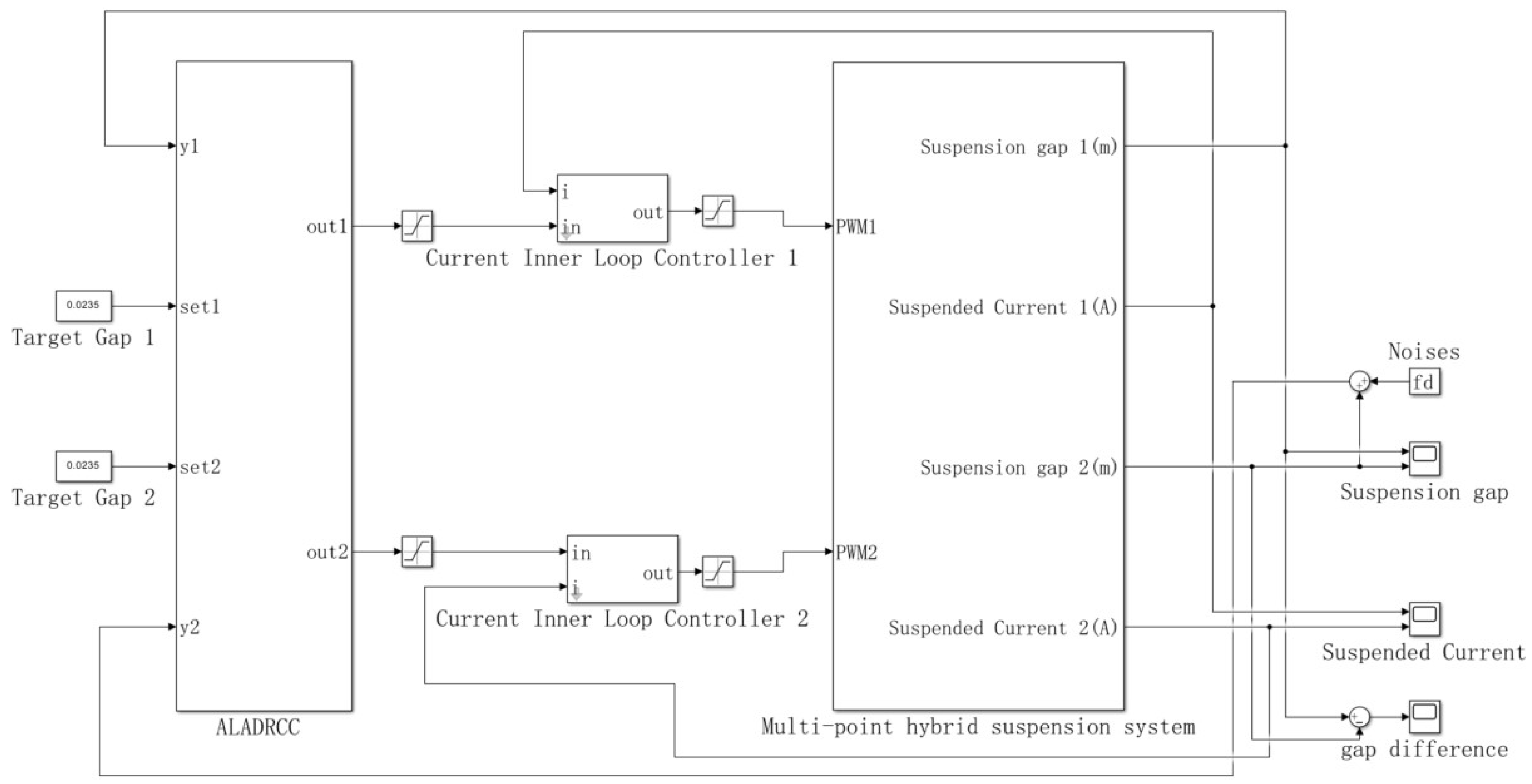
2.3. Multi-Point Hybrid Suspension System Model

For the overall suspension structure, the suspension electromagnets of the four suspension points are connected by rigid couplings, and each suspension point is independently formed into a closed-loop control loop, and the corresponding sensors are installed at both ends of the suspension frame for the measurement of the suspension gap and feedback control. Due to the restraining effect of the limiting wheels on both sides of the suspension frame, the suspension frame only generates undulating motion along the direction of a single degree of freedom during the suspension process. Therefore, there is no need to realize global synergistic control between the four suspension points, but only local synergistic output control for the two suspension points. Through the cooperative control of the two sides of the suspension points, the dynamic imbalance of the system under the unknown disturbance can be effectively suppressed, and the overall anti-disturbance capability and suspension stability of the system can be enhanced. Figure 3 shows the dynamics model of the unilateral hybrid suspension system, which describes the coupling relationship between the suspension electromagnet, the permanent magnet track, and the rigid connectors.

Where, $F_{e1}$ and $F_{e2}$ are the electromagnetic levitation force of the two suspension points; $F_{p1}$ and $F_{p2}$ are the permanent magnetic levitation force of the two suspension points; $M$ is the mass of the unilateral suspension frame; ${\delta }_1$ and ${\delta }_2$ are the suspension gaps of the two suspension points; $l$ is the distance from the center of mass $O$ to the center of the suspension point; and $\theta$ is the pitch angle of the rotation of the suspension frame.

For the unilateral hybrid suspension system model, the following assumptions are made to facilitate the qualitative analysis:

(1)

The mass of the unilateral suspension frame is uniformly distributed throughout its structure, and the center of gravity coincides with its geometric center;

(2)

There is no coupling between the permanent magnetic field and the electromagnetic field;

(3)

The suspension is rigid and undeformed, and the effect of transverse force is neglected;

(4)

Neglect of remanent magnetism, remanent magnetization, magnetic saturation phenomena, and no magnetic leakage.

The following is satisfied because the pitch angle of the unilateral suspension frame rotation is small:

$$\theta \approx \tan \theta ={\displaystyle \frac{{\delta }_2-{\delta }_1}{2l}}$$

(7)

$$\cos \theta \approx 1$$

(8)

The values of ${\delta }_1$ and ${\delta }_2$ can be measured directly by the gap sensor. Let the displacement of the unilateral suspension in the vertical direction be ${\delta }_g$, and the displacement in the direction of rotation about the center of mass be ${\delta }_{\theta }$. The relationship between ${\delta }_g$, ${\delta }_{\theta }$ and ${\delta }_1$, ${\delta }_2$ can be expressed as follows:

$$\left\{\begin{array}{l}{\delta }_g={\displaystyle \frac{{\delta }_1+{\delta }_2}{2}}\\ {\delta }_{\theta }=l·\theta ={\displaystyle \frac{{\delta }_2-{\delta }_1}{2}}\end{array}\right.$$

(9)

To characterize the motion of the unilateral suspension, it is necessary to establish the kinetic equations of the unilateral suspension moving along the center of mass and rotating around the center of mass. Let the suspension force $F_1=F_{e1}+F_{p1}, F_2=F_{e2}+F_{p2}$ be applied to the two suspension points; the combined force of the unilateral suspension frame in the vertical direction can be expressed as follows:

$$F_g=F_1+F_2$$

(10)

Then, the dynamical equations for a unilateral suspension frame moving adjectively along the center of mass can be expressed as follows:

$$F_g=-M{\ddot{\delta }}_g=F_1+F_2$$

(11)

The magnitude of the torque of the unilateral suspension frame around the center of mass is as follows:

$$T_{\theta }=J\ddot{\theta }={\displaystyle \frac{J{\ddot{\delta }}_{\theta }}{l}}=F_1·l\cos \theta -F_2·l\cos \theta$$

(12)

Defining the equivalent rotating mass $M_{\theta }=J/l^2$, the dynamical equations for the rotation of a unilateral suspension around the center of mass can be expressed as follows:

$$F_{\theta }=-M_{\theta }{\ddot{\delta }}_{\theta }=F_2-F_1$$

(13)

Then, the motion characteristics in the motion coordinate system of the unilateral suspension frame can be expressed as follows:

$$\left.\left[\begin{array}{c}{F}_g\\ F_{\theta }\end{array}\right.\right]=\left[\begin{array}{cc}-M& 0\\ 0& -M_{\theta }\end{array}\right]\left[\begin{array}{c}{\ddot{\delta }}_g\\ {\ddot{\delta }}_{\theta }\end{array}\right]$$

(14)

In summary, the unilateral suspension frame dynamics equation in the sensor coordinate system can be obtained as follows:

$$\left[\begin{array}{c}{\ddot{\delta }}_1\\ {\ddot{\delta }}_2\end{array}\right]=\left[\begin{array}{cc}-{\displaystyle \frac{1}{M}}-{\displaystyle \frac{1}{M_{\theta }}}& -{\displaystyle \frac{1}{M}}+{\displaystyle \frac{1}{M_{\theta }}}\\ -{\displaystyle \frac{1}{M}}+{\displaystyle \frac{1}{M_{\theta }}}& -{\displaystyle \frac{1}{M}}-{\displaystyle \frac{1}{M_{\theta }}}\end{array}\right]\left[\begin{array}{c}{F}_1\\ F_2\end{array}\right]$$

(15)

From the fact that the transformation matrix of Equation (15) is a non-diagonal array, it can be judged that there is a coupling relationship between the two suspension points of the unilateral hybrid suspension system. This coupling relationship implies that the change in the suspension gap of one suspension point will influence the suspension force of the other suspension point, which in turn affects the control performance of the whole system.

Joint Equations (5) and (15) lead to the block diagram of the open-loop model of the unilateral hybrid suspension system, as shown in Figure 4.

Assuming that the parameters of the two suspension electromagnets on one side are the same and the state variables of the system selected as the position, velocity, and current deviation of the two suspension points, the state space expression of the unilateral permanent magnet electromagnetic hybrid suspension system is as follows:

$$\left\{\begin{array}{l}\dot{x}=\left[\begin{array}{cccccc}0& 1& 0& 0& 0& 0\\ a_{21}& 0& a_{23}& a_{24}& 0& a_{26}\\ 0& a_{32}& a_{33}& 0& 0& 0\\ 0& 0& 0& 0& 1& 0\\ a_{51}& 0& a_{53}& a_{54}& 0& a_{56}\\ 0& 0& 0& 0& a_{65}& a_{66}\end{array}\right]x+\left[\begin{array}{cc}0& 0\\ 0& 0\\ b_{31}& 0\\ 0& 0\\ 0& 0\\ 0& b_{62}\end{array}\right]u+\left[\begin{array}{c}0\\ f_{d1}\\ 0\\ 0\\ f_{d2}\\ 0\end{array}\right]\\ y=\left[\begin{array}{cccccc}1& 0& 0& 0& 0& 0\\ 0& 0& 0& 1& 0& 0\end{array}\right]x\end{array}\right.$$

(16)

where $a_{21}=a_{54}=-{\displaystyle \frac{k_{e\delta }+k_{p\delta }}{M}}-{\displaystyle \frac{k_{e\delta }+k_{p\delta }}{M_{\theta }}}$, $a_{24}=a_{51}=-{\displaystyle \frac{k_{e\delta }+k_{p\delta }}{M}}+{\displaystyle \frac{k_{e\delta }+k_{p\delta }}{M_{\theta }}}$, $a_{23}=a_{56}=-{\displaystyle \frac{k_{ei}}{M}}-{\displaystyle \frac{k_{ei}}{M_{\theta }}}$, $a_{26}=a_{53}=-{\displaystyle \frac{k_{ei}}{M}}+{\displaystyle \frac{k_{ei}}{M_{\theta }}}$, $a_{32}=a_{65}={\displaystyle \frac{k_{ei}}{L_0}}$, $a_{33}=a_{66}=-{\displaystyle \frac{R}{L_0}}$, $b_{31}=b_{62}={\displaystyle \frac{1}{L_0}}$.

The mathematical model of the system is determined by combining the parameters of the physical platform, and the parameters of the control object model are shown in

Table 1. Parameters of the control object model.

Parameter	Value
$m/$$\mathrm{kg}$	17.6
$M/$$\mathrm{kg}$	35.2
$J/$$\mathrm{k}\mathrm{g}*{\mathrm{m}}^2$	3
$l/$$\mathrm{m}$	0.4
$N$	500
$R/$$\Omega$	2.4
$A/$${\mathrm{m}}^2$	0.005
${\mu }_0/$$(\mathrm{H}/\mathrm{m})$	$4\pi \times {10}^{-7}$
${\delta }_0/$$\mathrm{m}\mathrm{m}$	23
${\delta }^{*}/$$\mathrm{m}\mathrm{m}$	23.5
$g/$$(\mathrm{N}/\mathrm{k}\mathrm{g})$	9.8

.

Substituting the parameters in Table 1 yields the equivalent mass $M_{\theta }$ = 18.75 kg for the pitch mode, and then combining with Equation (15) yields the specific expression for the dynamics equation of the unilateral suspension frame in the sensor coordinate system as:

$$\left[\begin{array}{c}{\ddot{\delta }}_1\\ {\ddot{\delta }}_2\end{array}\right]=\left[\begin{array}{cc}-0.0817& 0.0249\\ 0.0249& -0.0817\end{array}\right]\left[\begin{array}{c}{F}_1\\ F_2\end{array}\right]$$

(17)

3. Controller Design

The core objective of the control of the hybrid suspension system is to achieve constant gap control, i.e., to ensure that the suspension gap is error-free and stable in real time with respect to the set value. The key to achieving this goal is to accurately control the voltage of the electromagnetic coil and thus indirectly regulate its current to ensure stable suspension of the system. Dynamic analysis shows that the hybrid levitation system has a third-order response, mainly due to the inductive property of the electromagnetic coil, which causes a slight hysteresis of the current change to the voltage adjustment.

To improve the dynamic response performance of the system and realize fast and accurate suspension control, this paper adopts the serial closed-loop control structure [21]. The block diagram of series-level closed-loop control for designing the multi-point hybrid suspension system is shown in Figure 5.

The structure includes two levels of feedback control: the outer loop is based on the suspension gap feedback, which is mainly responsible for real-time adjustment of the suspension gap to ensure that the system maintains a stable suspension state under different working conditions; the inner loop is based on the suspension current feedback, which is used to quickly adjust the suspension current and improve the dynamic response speed of the system. The series closed-loop control strategy can effectively overcome response hysteresis and realize fast and stable suspension regulation, thus improving the overall control performance of the system.

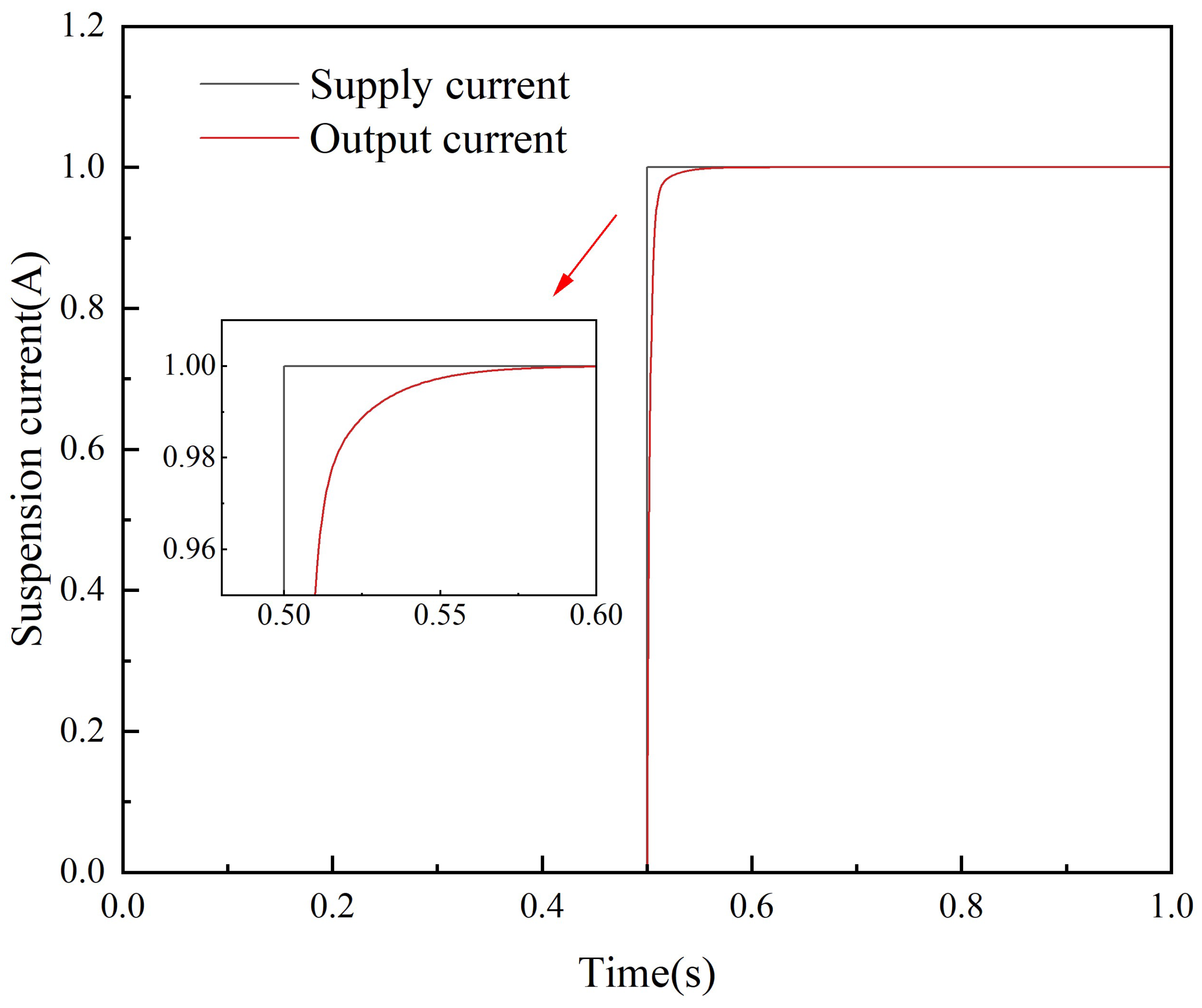
3.1. Current Inner Loop PI Controller Design

From Equation (4), the hybrid suspension system is a third-order system with voltage input, while it exhibits second-order characteristics with current input. Given the limitations of chopper circuits that directly control the voltage at the ends of the electromagnetic coil, the system has a higher complexity of controller design if the current is used as input. To reduce the design difficulty and improve the system performance, this study introduces a current loop to down-order the system by analyzing the conversion relationship between voltage and current. According to Table 1, the static inductance of the electromagnet is 0.033 H, and the internal resistance is 2.4 Ω, while the experimental platform voltage is 24 V, and the PWM amplitude is 1000, such that the open-loop transfer function of the suspension electromagnet can be obtained as follows:

$$G(s)={\displaystyle \frac{24}{1000}}·{\displaystyle \frac{1}{0.033s+2.4}}$$

(18)

A PI controller with $K_P=500, K_I=30000$ is designed, and a step signal of 1 A is applied at 0.5 s. The current tracking simulation waveform is shown in Figure 6.

In the face of a 1 A step response, the current rise time is about 55 ms with no overshoot, which satisfies the control requirements of the suspension system. After the current loop, the system can be approximated as a second-order system with current control as follows:

$$\left\{\begin{array}{l}m{\displaystyle \frac{d^2{\delta }_i\left(t\right)}{d{t}^2}}=F_i\left(i_i,{\delta }_i\right)-mg+f_{di}(t)\\ F_i\left(i_i,{\delta }_i\right)={\displaystyle \frac{{\mu }_0{N}^{2}S}{4}}{\displaystyle \frac{u_i\left(t\right)}{{\delta }_i^2(t)}}+k{e}^{b{\delta }_i(t)}+\mathrm{c}\\ u_i\left(t\right)=i_i^2\left(t\right)\end{array}\right.$$

(19)

3.2. Gap Outer Loop ALADRCC Controller Design

The synchronized coordinated control problem of a multi-point hybrid suspension system considering coupled disturbances is transformed into a problem of synchronized control of the suspension gap and velocity of two suspension points. The second-order hybrid suspension system is rewritten in the form of an integral-type system by considering unmodeled dynamics and unknown disturbances as follows:

$$\left\{\begin{array}{l}{\dot{x}}_{i1}=x_{i2}\\ {\dot{x}}_{i2}=f_i(x_{i1},x_{i2},w_i,t)+b_i{u}_i\\ y_i=x_{i1}\end{array}\right.$$

(20)

where $u_i$ is the system input, $x_{i1}, x_{i2}$ is the system state variable, $y_i$ is the system output, $w_i$ is the external disturbance, and $b_i$ is the system control gain. $b_i$ will take the approximate value of $b_{0i}$, and the uncertainty part is defined as the total disturbance $x_{i3}=f_i(x_{i1},x_{i2},w_i,t)+(b_i-b_{0i})u_i$, then the new state equation of the system is as follows:

$$\left\{\begin{array}{l}{\dot{x}}_{i1}=x_{i2}\\ {\dot{x}}_{i2}=x_{i3}+b_{0i}{u}_i\\ x_{i3}=f_i(x_{i1},x_{i2},w_i,t)+(b_i-b_{0i})u_i\\ y_i=x_{i1}\end{array}\right.$$

(21)

The tracking differentiator (TD) is used to smooth out abrupt signals, avoiding overshoots and oscillations induced by the system’s direct response to the abrupt changes while providing a smooth differential signal to reduce the effect of high-frequency noise on the controller. The discrete form expression of the designed TD is given by the following:

$$\left\{\begin{array}{l}{\tilde{\delta }}_i(k+1)={\tilde{\delta }}_i(k)+h{\dot{\tilde{\delta }}}_i(k)\\ {\dot{\tilde{\delta }}}_i(k+1)={\dot{\tilde{\delta }}}_i(k)+hfhan({\tilde{\delta }}_i(k)-{\delta }_i(k),{\dot{\tilde{\delta }}}_i(k),r_0,h_0)\end{array}\right.$$

(22)

where ${\tilde{\delta }}_i$ is the tracking signal output by TD; ${\dot{\tilde{\delta }}}_i$ is the differential signal output by TD; $h$ is the integration step; $h_0$ is the filtering factor; $r_0$ is the velocity factor; and $fhan(x)$ is the maximum velocity synthesis function.

The linear expansion state observer (LESO) can estimate the system state and the total disturbance in real time, which can improve the system’s disturbance immunity without changing the control structure. The system state observation errors are defined as follows, respectively:

$$\left\{\begin{array}{l}{e}_{i1}=z_{i1}-x_{i1}\\ e_{i2}=z_{i2}-x_{i2}\\ e_{i3}=z_{i3}-x_{i3}\end{array}\right.$$

(23)

where $e_{i1}$ is the gap observation error; $e_{i2}$ is the velocity observation error; $e_{i3}$ is the disturbance observation error; and $z_{i1}, z_{i2}, z_{i3}$ denotes the LESO observations of the suspension gap at the suspension point, the velocity of the suspension gap change, and the total disturbance, respectively.

To alleviate the contradiction caused by the traditional LESO bandwidth selection while considering the dynamic response capability and noise rejection of the system, the expression of the adaptive linear expansion state observer (ALESO) is designed as follows:

$$\left\{\begin{array}{l}{\dot{z}}_{i1}=z_{i2}-{\beta }_{i1}{e}_{i1}, {\beta }_{i1}=3{\omega }_{0i}\\ {\dot{z}}_{i2}=z_{i3}+b_{0i}{u}_i-{\beta }_{i2}{e}_{i1}, {\beta }_{i3}=3{\omega }_{0i}^2\\ {\dot{z}}_{i3}=-{\beta }_{i3}{e}_{i1}, {\beta }_{i3}={\omega }_{0i}^3\\ {\omega }_{0i}={\omega }_{0i\min }+({\omega }_{0i\max }-{\omega }_{0i\min })\tanh (k_{\omega }\left|e_{i1}\right|)\end{array}\right.$$

(24)

where ${\omega }_{0i\min }\le {\omega }_{0i}\le {\omega }_{0i\max }$, ${\omega }_{0i\min }$ is the minimum bandwidth to suppress noise and ensure steady-state accuracy; ${\omega }_{0i\min }$ is the maximum bandwidth to speed up the response and reduce the observation error; ${\beta }_{i1}$, ${\beta }_{i2}$ and ${\beta }_{i3}$ are the gain coefficients of ALESO; $\tanh (x)$ is the hyperbolic tangent function; $k_{\omega }$ is the adaptive factor, which adjusts the rate of change of the bandwidth and takes a positive value. The block diagram of the structure of ALESO is shown in Figure 7.

The expression of Coupling Cooperative Compensator (CCC) is further designed as:

$$\left\{\begin{array}{l}{\epsilon }_1=z_{21}-z_{11}\\ {\dot{\epsilon }}_1=z_{22}-z_{12}\\ {\epsilon }_2=z_{11}-z_{21}\\ {\dot{\epsilon }}_2=z_{12}-z_{22}\end{array}\right.$$

(25)

where $i=1, 2$, ${\epsilon }_i$, ${\dot{\epsilon }}_i$ denote the suspension gap synchronization error and velocity synchronization error of the two suspension points, respectively.

The system takes the state deviation as input and designs the error cross-coupling-based linear feedback cooperative control rate (CLSEF) as follows:

$$u_{0i}=k_1({\tilde{\delta }}_i-z_{i1})+k_2({\dot{\tilde{\delta }}}_i-z_{i2})+c_1{\epsilon }_i+c_2{\dot{\epsilon }}_i$$

(26)

where $k_1$, $k_2$ represent the feedback control coefficients; $c_1$, $c_2$ represent the cross-coupling coefficients; and e represents the intermediate control variable of the two suspension points. To facilitate the engineering parameterization, the feedback control coefficients $k_1={\omega }_c^2$, $k_2=2{\omega }_c$ are configured. On this basis, the total disturbance $z_{i3}$ is compensated into $u_i$ with a certain gain of $b_{0i}$. The actual control quantity output is obtained as follows:

$$u_i=u_{0i}-{\displaystyle \frac{z_{i3}}{b_{0i}}}$$

(27)

In summary, the block diagram of the ALADRCC algorithm structure is shown in Figure 8. ALESO is used for online estimation of suspension gap, velocity signal, and system perturbation, real-time observation of the system state, and compensation of system perturbation, in addition to improving the dynamic response and high-frequency noise suppression ability of the system, dynamically increasing the observer bandwidth to speed up the system response when the gap observation error is large, and dynamically decreasing the observer bandwidth to enhance the noise suppression ability when the gap observation error is small. CCC is used to calculate the suspension gap synchronization error and velocity synchronization error of the two suspension points. CLSEF is used to provide feedback on the system state error and synchronization error to generate the corresponding control outputs to offset the system perturbation and realize cooperative control.

3.3. Parameter Calibration

For each suspension point, the parameters to be tuned are two parameters for the PI controller ($K_P,K_I$), three parameters for the TD ($h,h_0,r_0$), three parameters for the ALESO (${\omega }_{0\max },{\omega }_{0\min },k_w$), and four parameters for the CLSEF (${\omega }_c,b_0,c_1,c_2$).

(1)

According to the simulation in Section 3.1, it can be seen that $K_P=500, K_I=30000$, which can satisfy the current tracking performance requirements of the suspension system.

(2)

The sampling period is set to 0.5 ms, then the sampling step size $h=0.0005$ s; $h_0$ increase can enhance the filtering effect, increase when the noise is large, and decrease when the response is slow, with a typical range of 0.1~2.0; $r_0$ increase can speed up the tracking speed, but too large will cause oscillations, according to the set value of the change in the frequency of the adjustment, with a typical range of 50~300.

(3)

An increase in the value of ${\omega }_0$ improves the system response, but too much of it would introduce the effect of high-frequency noise. The value of ${\omega }_{0\max }$ should ensure that the system has good dynamic performance and fast responses when disturbed to be selected according to the actual system; ${\omega }_{0\min }$ should ensure that the system has good steady-state performance and that the suspension gap fluctuations and current ripple are small when the system is stabilized, ensuring low noise sensitivity, to be selected according to the actual system; For $k_{\omega }$, the larger the bandwidth, the faster the response speed; this paper uses the simulation and experimental selection of $k_{\omega }$ = 2.

(4)

${\omega }_c$ is the controller bandwidth. According to the relationship between the response of the closed-loop system and the performance index, the regulation formula of ${\omega }_c$ can be expressed as follows: ${\omega }_c=4/t_s$, where $t_s$ is the system rise time. In the case of incomplete model information, $b_0$ is usually set as a large initial value, then ${\omega }_c$ and ${\omega }_o$ are adjusted to make the system stable. Then, the value of $b_0$ is gradually reduced to optimize the system’s immunity to disturbances and the dynamic response performance. $c_1, c_2$ are the system cross-coupling coefficients, the corresponding value of zero indicates independent control of multiple points; the larger the corresponding value is, the more synergistic it is, but the value is too large to cause system oscillations. For the cross-coupling coefficients of the system, the larger the corresponding value, the stronger the synergy, but values that are too large will cause system oscillation. Rectification time should be gradually increased under the premise of ensuring the stability of the system.

4. Simulation Analysis

The control models of single-point and multi-point hybrid suspension systems are built in MATLAB R2024a/Simulink, respectively. The parameters of the control algorithm are tuned based on the experience of tuning parameters, and the effectiveness and superiority of the designed ALESO and CCC are verified through simulation experiments.

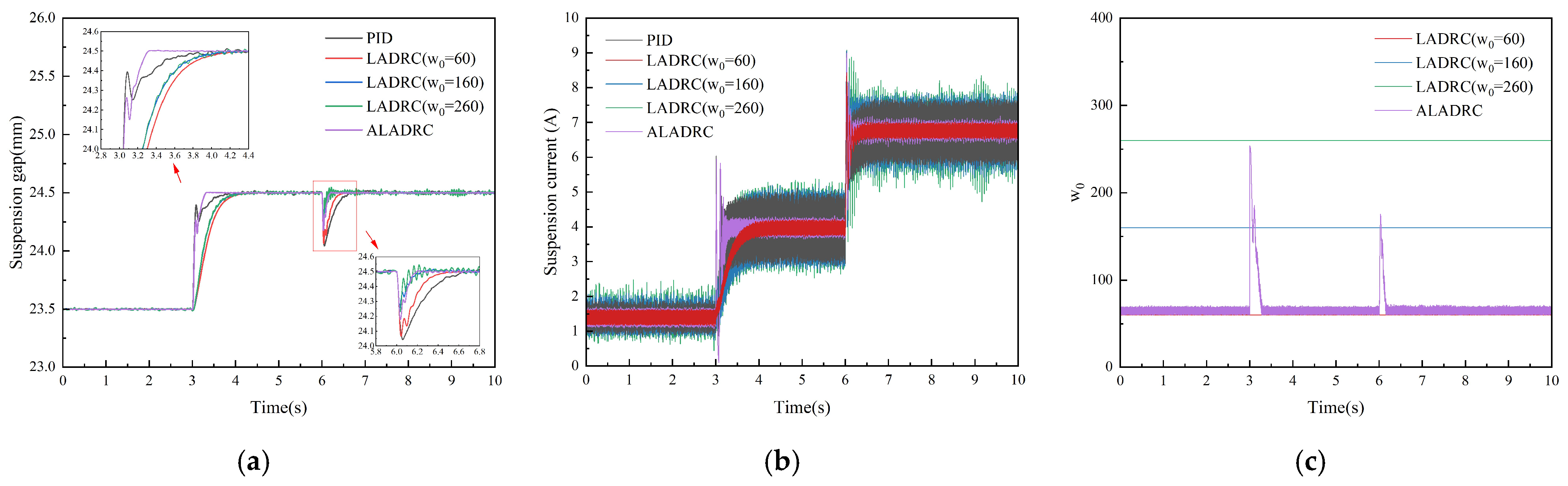
4.1. Single-Point Suspension Immunity Simulation Experiment

To verify the effectiveness of the designed ALESO, the immunity simulation experiments are carried out by comparing the ALADRC with the PID and the traditional LADRC control algorithms with different bandwidths, respectively. The single-point hybrid suspension system control simulation model shown in Figure 9 is constructed. The same parameter configuration is used for the current inner loop except for the position of the outer loop, which uses the three different control algorithms mentioned above, with $K_p=500, K_I=30000$, to ensure the fairness of the experimental comparison results.

The parameters of the designed control algorithms are fully adjusted to ensure that each algorithm can achieve the best control effect under the same experimental conditions. The parameters of the control algorithms for the single-point suspension immunity simulation experiment are shown in

Table 2. Control algorithm parameters for single-point suspension immunity simulation experiments.

PID	LADRC	ALADRC
$\begin{array}{l}{K}_p=9000\\ K_i=30000\\ K_d=700\end{array}$	$\begin{array}{l}h=0.0005\\ h_0=0.045\\ r_0=100\\ {\omega }_c=35\\ {\omega }_0=60/160/260\\ b_0=0.2\end{array}$	$\begin{array}{l}h=0.0005\\ h_0=0.045\\ r_0=100\\ {\omega }_c=35\end{array}$ $\begin{array}{l}{\omega }_{0\max }=260\\ {\omega }_{0\min }=60\\ k_{\omega }=2\\ b_0=0.2\end{array}$

.

A random noise with uniformly distributed amplitude ±5 μm and a sinusoidal noise with amplitude 20 μm and angular frequency 500 rad/s are superimposed in the feedback loop of the target suspension gap to simulate the measurement noise interference in the actual operation environment. The simulation experiments are set as follows: The initial target suspension gap is set to 23.5 mm, and a step signal is applied at 3 s to make the target suspension gap change from 23.5 mm to 24.5 mm to verify the tracking performance of the controller. The suspension mass is increased by 2 kg at 6 s to simulate the external load perturbation and verify the algorithm’s suppression capability of the perturbation. The results of the simulation are shown in Figure 10.

The suspension gap response curves from Figure 10a show that all three control algorithms can achieve perturbation suppression stabilized at the target suspension gap, but there are differences in the control performance. Specifically, under PID control, the regulation time of the step response is 861 ms, the regulation time under load perturbation is 616 ms, and the peak value of suspension gap fluctuation is 0.456 mm. Using the traditional LADRC algorithm control, the system tracking response speed is accelerated with the increase in the observer bandwidth in a suitable range. However, the system noise also increases, and the traditional LADRC algorithm control is also suitable for the traditional LADRC algorithm control with the observer bandwidths of 60 rad/s, 160 rad/s, and 260 rad/s, which correspond to the selected bandwidths, respectively. Under the control of the traditional LADRC algorithm with the observer bandwidths of 60 rad/s, 160 rad/s, and 260 rad/s, the regulation times of the system step response are 1187 ms, 1014 ms, and 1007 ms, respectively, the regulation times under the load disturbance are 450 ms, 225 ms, and 122 ms, respectively, and the peak values of the suspension gap fluctuation are 0.429 mm, 0.276 mm, and 0.241 mm, respectively. ALADRC algorithm control, the regulation time of the system step response is the fastest at 320 ms, the regulation time under load disturbance is 179 ms, and the peak value of suspension gap fluctuation is 0.321 mm. Compared with the traditional high-bandwidth LADRC, the ALADRC shows a significant advantage in noise suppression, and this feature is of great significance for improving the control performance of the hybrid suspension system. Further observation of the suspension current response curves in Figure 10b shows that in the step response and load disturbance phases, the steady-state current ripple of the PID control is 1.997 A and 1.926 A. In comparison, under the control of the conventional LADRC algorithm with observer bandwidths chosen to correspond to 60 rad/s, 160 rad/s, and 260 rad/s, the steady-state current ripples are 0.444 A, 2.273 A, and 2.663 A in the step response phase, and 0.525 A, 2.444 A, and 3.041 A in the load disturbance phase, respectively. The steady-state current ripple in the load disturbance stage is 0.525 A, 2.444 A, and 3.041 A. The steady-state current ripples in the step response and load disturbance stages are 0.557 A and 0.754 A, respectively, when using ALADRC control. Figure 10c shows the adaptive response curve of ALADRC, and the observer bandwidth of ALADRC can adapt to the system perturbation changes in both the step response stage and the load change adaptation stage. The performance of control algorithms for single-point suspension immunity simulation experiments is shown in

Table 3. Control algorithm performance for single-point suspension immunity simulation experiments.

Performance		PID	LADRC (${\mathit{\omega }}_0$ = 60)	LADRC (${\mathit{\omega }}_0$ = 160)	LADRC (${\mathit{\omega }}_0$ = 260)	ALADRC
(1) Step response	Regulation time	861 ms	1187 ms	1014 ms	1007 ms	320 ms
	Maximum fluctuation	0.456 mm	0.429 mm	0.276 mm	0.241 mm	0.321 mm
	Steady-state current ripple	1.997 A	0.444 A	2.273 A	2.663 A	0.557 A
(2) Load perturbation	Regulation time	616 ms	450 ms	225 ms	122 ms	179 ms
	Maximum fluctuation	0.456 mm	0.429 mm	0.276 mm	0.241 mm	0.321 mm
	Steady-state current ripple	1.926 A	0.525 A	2.444 A	3.041 A	0.754 A

, and the results show that the ALADRC control algorithm exhibits advantages in both dynamic and static performance. Compared with the traditional LADRC algorithm, it integrates the low noise sensitivity of the small observer bandwidth and the strong disturbance adaptation capability of the large observer bandwidth, which not only has a faster system response speed and can quickly track the target suspension gap changes but also has a stronger suppression capability of the measurement noise and the external perturbation under the complex working conditions, and improves the performance of the LADRC control algorithm. At the same time, it has a stronger suppression ability for measuring noise and external disturbance under complex working conditions, which improves the accuracy and anti-interference performance of the system’s steady state.

4.2. Multi-Point Suspension Synergy Simulation Experiment

To verify the effectiveness of CCC, a multi-point hybrid suspension system control simulation model is constructed, multi-point suspension synergy simulation experiments are conducted, and the simulation model is shown in Figure 11.

The parameters of the ALADRC algorithm for each suspension point are the same, and the parameters that have been changed from the single-point simulation experiments through further calibration are: ${\omega }_c=15, {\omega }_{0\max }=460, {\omega }_{0\min }=260$. The experimental setup is as follows: the target suspension gap is 23.5 mm, the position of the suspension point 2 is superimposed with ±5 μm uniformly distributed noise, and 100 N, vertically downward interference is applied at t = 3 s, and the interference is withdrawn at t = 6 s, and the suspension point 1 is kept unchanged without any perturbation, and the results of the multi-point levitation synergy simulation experiments are shown in Figure 12, which is obtained by the cross-coupling coefficient of $c_1=0, c_2=0$.

Figure 12 shows that when the CCC does not work, and the system is controlled only by the ALADRC algorithm of the two suspension points, the outputs of the two suspension points deviate greatly. Under the interference of 100 N, the suspension gap of suspension point 2 is shifted by 0.623 mm. Meanwhile, the floating gap of suspension point 1 is shifted by 0.115 mm due to the coupling characteristics of the mechanical structure, and the peak fluctuation values of the suspension gap of suspension point 2 and suspension point 1 when the interference is withdrawn are 0.513 mm and 0.119 mm, and the differences of the two suspension points in terms of the suspension gaps are 0.535 mm and 0.398 mm, at this time, the outputs of the two suspension points deviate greatly. 0.535 mm and 0.398 mm when the interference is applied and withdrawn. At this time, there is no synergy between the two suspension points, and the change in the suspension gap only shows the coupling characteristics. The values of the cross-coupling coefficients $c_1, c_2$ increase when the cross-coupling coefficients are $c_1=100, c_2=0.1$. The multi-point suspension synergy simulation results are shown in Figure 13.

As can be seen from Figure 13, the peaks of suspension gap fluctuations of suspension point 2 and suspension point 1 are 0.617 mm and 0.167 mm when the interference is applied, and the peaks of suspension gap fluctuations of suspension point 2 and suspension point 1 are 0.479 mm and 0.141 mm when the interference is withdrawn, and the peaks of the difference in the suspensions of suspension gaps of the two suspension points are 0.520 mm and 0.371 mm when the interference is applied and withdrawn, respectively. Compared with Figure 11, it is reduced, and the two suspension points produce a coordinated and synchronized trend. The values of the cross-coupling coefficient $c_1, c_2$ continue to increase when the cross-coupling coefficient $c_1=1000, c_2=0.1$. The results of the multi-point suspension synergy simulation are shown in Figure 14.

As can be seen in Figure 14, with the increase in the values of the cross-coupling coefficients $c_1, c_2$, the synergy of the two suspension points is further strengthened, and the peaks of suspension gap fluctuation of suspension point 2 and suspension point 1 are 0.588 mm and 0.384 mm, respectively, when the interference is applied. The peaks of suspension gap fluctuation of suspension point 2 and suspension point 1 when the interference is withdrawn are 0.373 mm and 0.268 mm, and the peaks of suspension gap difference of the two suspension points when interference is applied and withdrawn are 0.426 mm and 0.233 mm, respectively. The peak values of the gap difference are 0.426 mm and 0.233 mm when the interference is applied and withdrawn, respectively, which are 20.37% and 42.04% lower than the peak values of the gap difference when the synergistic control is not added in Figure 11, which verifies the effectiveness of the designed CCC.

5. Results

To prove the above theoretical and simulation analyses, a multi-point hybrid levitation experimental platform was built in the laboratory, as shown in Figure 15. The experimental platform mainly consists of a DC power supply, suspension controller, suspension chopper, gap sensor, and suspension frame.

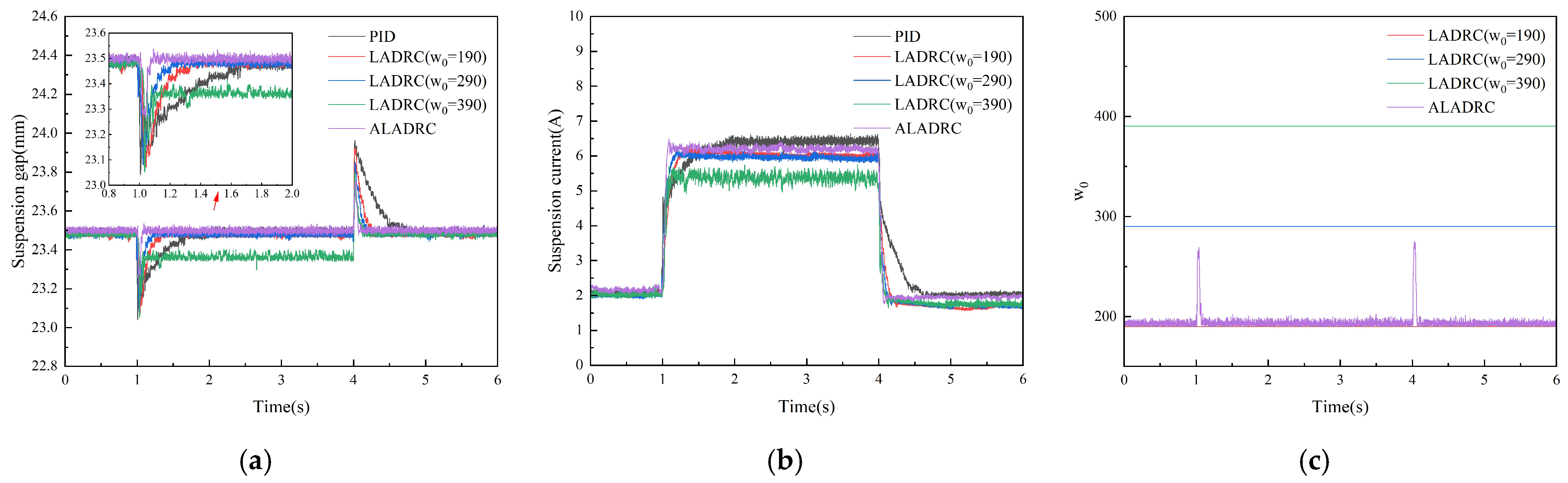
5.1. Single-Point Suspension Immunity Experiment

To verify the effectiveness of the designed ALADRC control algorithm, suspension point 1 is selected on the hybrid suspension experimental platform for single-point suspension immunity experiments. Considering the difference in the order of magnitude of the suspension gap variables between the simulation experiment and the physical experiment, combined with the previous analysis results and the actual system characteristics, the control parameters are re-adjusted to make them more consistent with the operational requirements of the physical system. The control algorithm parameters for single-point suspension immunity experiments are shown in

Table 4. Control algorithm parameters for single-point suspension immunity experiments.

PID	LADRC	ALADRC
$\begin{array}{l}{K}_p=11\\ K_i=5\\ K_d=0.3\end{array}$	$\begin{array}{l}h=0.001\\ h_0=0.01\\ r_0=100\\ {\omega }_c=5\\ {\omega }_0=190/290/390\\ b_0=1.5\end{array}$	$\begin{array}{l}h=0.001\\ h_0=0.01\\ r_0=100\\ {\omega }_c=5\end{array}$$\begin{array}{l}{\omega }_{0\max }=390\\ {\omega }_{0\min }=190\\ k_{\omega }=2\\ b_0=1.5\end{array}$

. The same parameter configuration is used for all three algorithms’ current inner loops: $K_p=200, K_I=800$.

The experiment was set up as follows: a load of about 2 kg was suddenly applied to the position of suspension point 1 at 1 s, and the load was quickly removed after holding it for the present period. The experimental results were recorded, as shown in Figure 16.

From the suspension gap response curves in Figure 16a, the effects of various control algorithms on the system response are different in the case of a sudden addition of a 2 kg load at 1 s. The peak value of the suspension gap fluctuation under PID control is the largest, reaching 1.959 mm and returning to the steady state after about 632 ms. Under the traditional LADRC algorithm with observer bandwidths of 190 rad/s and 290 rad/s, the peak suspension gap fluctuations are 1.928 mm and 1.919 mm, respectively, and the regulation time is shortened to 365 ms and 226 ms, respectively. When the observer bandwidth is increased to 390 rad/s, the peak suspension gap fluctuation is 1.936 mm, the system load-bearing capacity decreases, and the suspension gap cannot be fully restored to the target value after applying a load. After applying the load, the levitation gap cannot be fully recovered to the target value. Combined with the single-point suspension simulation experiments, it can be concluded that increasing the observer bandwidth within a certain range can improve the dynamic response speed of the system, but beyond a certain range, it will weaken the control system stiffness, thus reducing the control performance. This problem can be solved when controlled by the ALADRC algorithm. Under the control of the ALADRC algorithm, the peak value of suspension gap fluctuation is significantly reduced to 1.726 mm, and the regulation time is greatly reduced to 91 ms. Figure 16b demonstrates the suspension current response characteristics. The steady-state current ripple at load disturbance under PID control is 0.494 A. Under the control of a conventional LADRC algorithm with observer bandwidths set to 190 rad/s, 290 rad/s, and 390 rad/s, respectively, the steady-state current ripple is reduced to 0.151 A, 0.242 A, and 0.486 A, respectively. Under the control of ALADRC, the steady-state current ripple is 0.212 A. From the observer bandwidth response curve of ALADRC in Figure 16c, it can be quickly adjusted according to the system state during the process of sudden load addition or removal, thus realizing dynamic adaptive optimization. The performance of control algorithms for single-point suspension immunity simulation experiments is shown in

Table 5. Control algorithm performance for single-point suspension immunity experiments.

Performance	PID	LADRC (${\mathit{\omega }}_0$ = 190)	LADRC (${\mathit{\omega }}_0$ = 290)	LADRC (${\mathit{\omega }}_0$ = 390)	ALADRC
Regulation time	632 ms	365 ms	226 ms	-	91 ms
Maximum fluctuation	1.959 mm	1.928 mm	1.919 mm	1.936 mm	1.726 mm
Steady-state current ripple	0.464 A	0.151 A	0.242 A	0.486 A	0.212 A

, and the experimental results show that the ALADRC control algorithm can quickly adjust the suspension gap to restore to the stable state when the load is suddenly added or removed, with the shortest adjustment time and the smallest fluctuation to the load perturbation, and the suspension current has a smoothness, which shows good robustness and anti-perturbation ability.

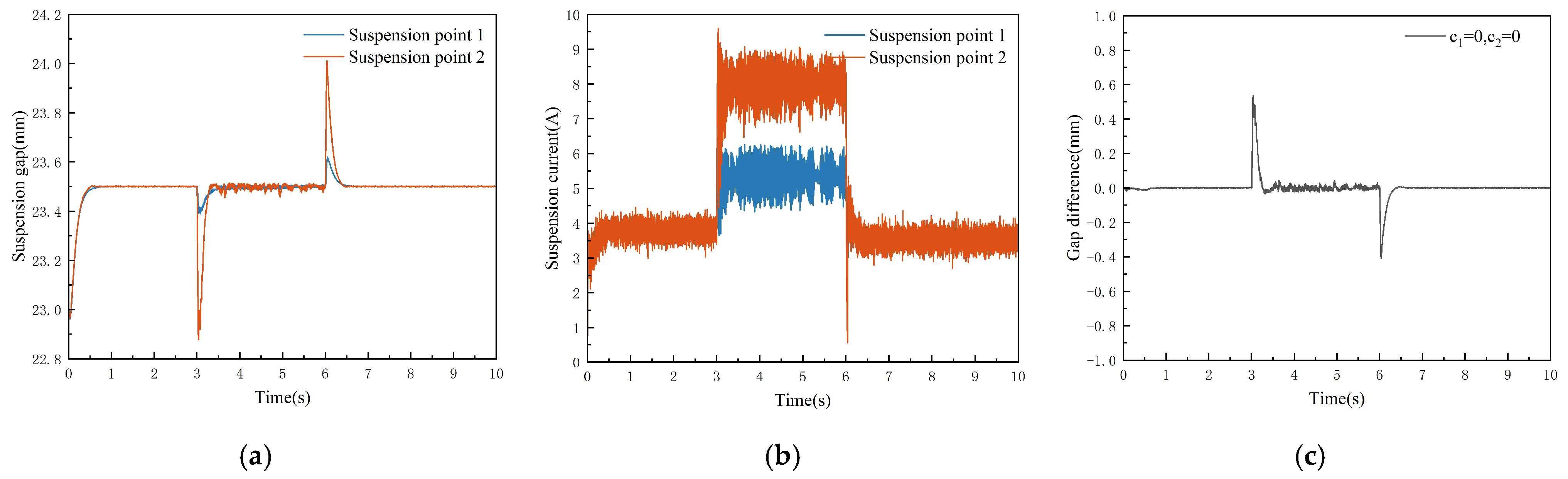
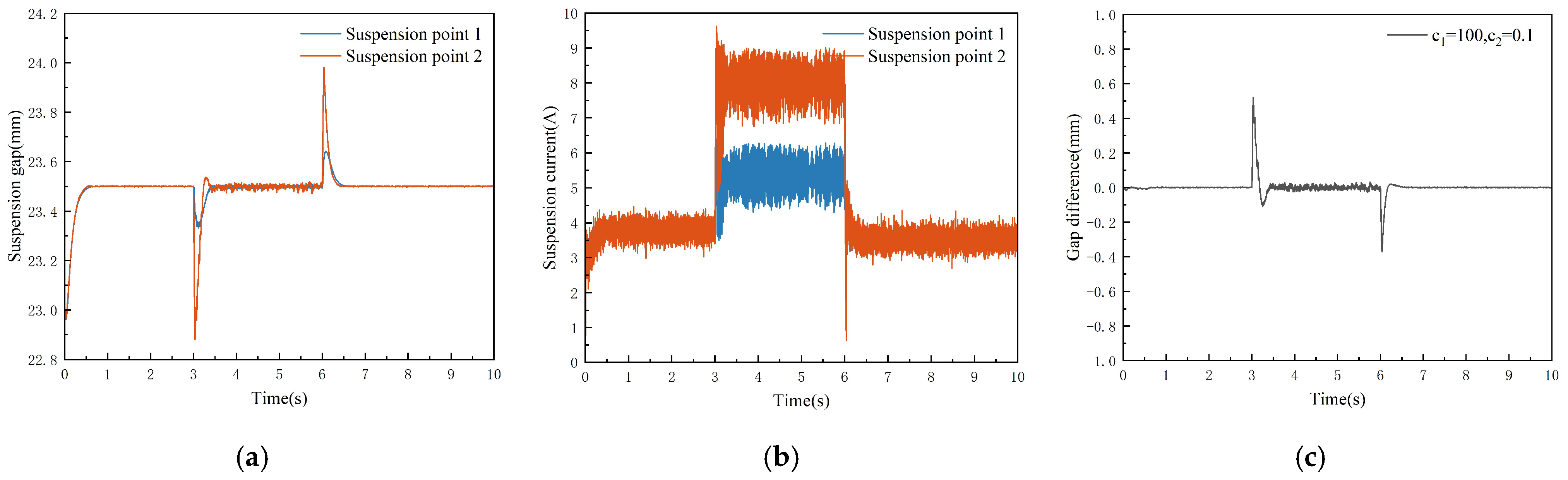
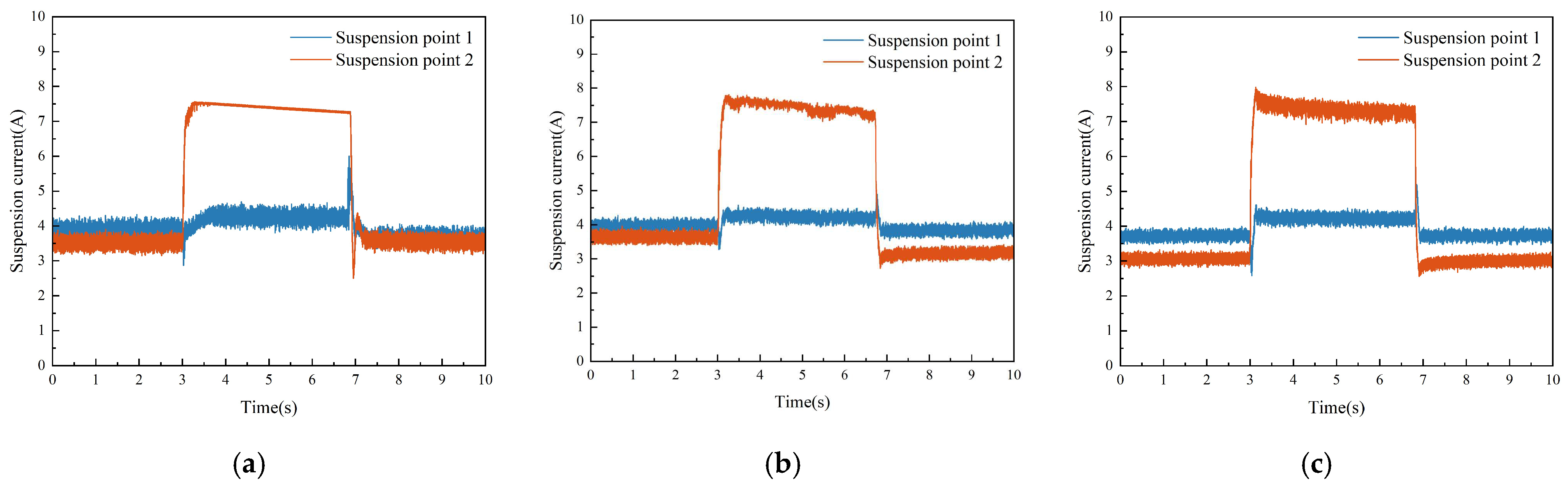
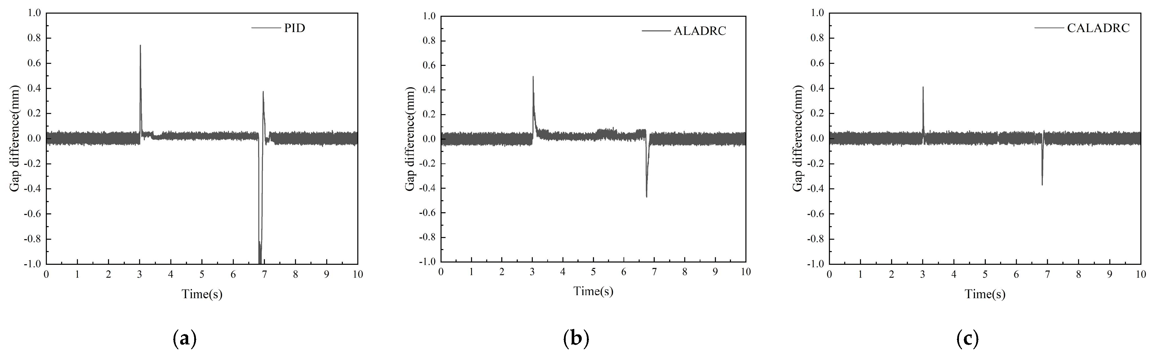
5.2. Unilateral Suspension Immunity Experiment

Based on the single-point suspension immunity experiments, the effectiveness of the designed ALESO is verified. To further verify the validity of the coupled CCC, the most widely used PID control, ALADRC, and ALADRCC in the industry are compared. The following suspension point 1 and suspension point 2 are selected on the multi-point hybrid suspension experimental platform for the unilateral suspension immunity experiment. Due to some differences in hardware characteristics between suspension point 1 and suspension point 2, the same control parameters show different control effects in different suspension points. Therefore, to ensure the fairness and comparability of the experiments, this paper carries out independent parameter tuning for the two suspension points to realize consistent control performance as much as possible. The algorithm parameters for the unilateral suspension immunity experiments are shown in

Table 6. Control algorithm parameters for unilateral suspension immunity experiments.

Suspension Point	PID	ALADRC	ALADRCC
1	$\begin{array}{l}{K}_p=9\\ K_i=10\\ K_d=0.31\end{array}$	$\begin{array}{l}h=0.001\\ h_0=0.01\\ r_0=100\\ {\omega }_c=5\end{array}$$\begin{array}{l}{\omega }_{0\max }=390\\ {\omega }_{0\min }=190\\ k_{\omega }=2\\ b_0=1.5\end{array}$	$\begin{array}{l}h=0.001\\ h_0=0.01\\ r_0=100\\ {\omega }_c=5\\ {\omega }_{0\max }=390\end{array}$$\begin{array}{l}{\omega }_{0\min }=190\\ k_{\omega }=2\\ b_0=1.5\\ c_1=80\\ c_2=0.1\end{array}$
2	$\begin{array}{l}{K}_p=4\\ K_i=10\\ K_d=0.29\end{array}$	$\begin{array}{l}h=0.001\\ h_0=0.01\\ r_0=100\\ {\omega }_c=5\end{array}$$\begin{array}{l}{\omega }_{0\max }=490\\ {\omega }_{0\min }=290\\ k_{\omega }=2\\ b_0=2.8\end{array}$	$\begin{array}{l}h=0.001\\ h_0=0.01\\ r_0=100\\ {\omega }_c=5\\ {\omega }_{0\max }=490\end{array}$$\begin{array}{l}{\omega }_{0\min }=290\\ k_{\omega }=2\\ b_0=2.8\\ c_1=80\\ c_2=0.1\end{array}$

.

The experiment was set up such that a load of about 2 kg was suddenly applied to the position of suspension point 2, maintained for a predetermined period, and then quickly withdrawn. The results were recorded as shown in the following figure.

Figure 17 shows the suspension gap response curve. Under the traditional PID control, the amplitude of the suspension gap fluctuation is 0.829 mm when a load is applied, and it returns to the steady state after about 157 ms. There is a steady-state error of 0.02 mm in suspension point 2 after it returns to the steady state, the amplitude of suspension gap fluctuation is 1.281 mm when the load is withdrawn, and the steady-state error disappears after it is withdrawn under the ALADRC algorithm. Under the control of the ALADRC algorithm, the amplitude of suspension gap fluctuation is 0.547 mm when a load is applied, and it returns to the steady state after about 175 ms. There is a steady-state error of 0.02 mm in suspension point 2 after it returns to the steady state, the amplitude of suspension gap fluctuation is 0.478 mm when the load is withdrawn, and the steady-state error disappears after the withdrawal of the load. The suspension gaps of the two points under the control of the ALADRCC algorithm are synchronized. The suspension gap fluctuation amplitude drops to 0.442 mm and returns to the steady state after about 126 ms, and there is no steady state error after returning to the steady state. The suspension gap fluctuation amplitude is 0.469 mm when the load is withdrawn. From the suspension current response curves in Figure 18, in the phase of loaded disturbance, the steady-state current fluctuations of the three control algorithms are all within 1 A, and the ALADRCC control enhances the current intensity at the point of suspension under load. Further observation of the relative suspension gap difference curves in Figure 19 shows that the peak value of the suspension gap difference between the two suspension points is 0.744 mm when the load is applied under PID control, and the peak value of the suspension gap difference between the two suspension points is 1.234 mm when the load is withdrawn, while the peak value of the suspension gap difference between the two suspension points is 0.511 mm when the load is applied and the peak value of the suspension gap difference between the two suspension points is 0.465 mm when the load is withdrawn under ALADRC control. The peak value of the suspension gap difference between the two levitation points under ALADRCC control is 0.465 mm when the load is applied and 0.413 mm when the load is removed, and the peak value of the suspension gap difference between the two levitation points under ALADRCC control is 0.269 mm. The performance of the control algorithm for the unilateral suspension immunity experiments is shown in

Table 7. Control algorithm performance for unilateral suspension immunity experiments.

Performance	PID	ALADRC	ALADRCC
Regulation time	157 ms	175 ms	126 ms
Maximum fluctuation	0.829 mm	0.547 mm	0.442 mm
Steady-state error	0.02 mm	0.02 mm	0
Steady-state current ripple	0.733 A	0.513 A	0.631 A
Maximum suspension gap difference	0.744 mm	0.511 mm	0.413 mm

. The experimental results show that when a single point is perturbed by the load, the suspension gaps of the two levitation points under ALADRCC control can maintain synchronized consistency, reduce the suspension gap difference between the two suspension points, and show good synergy.

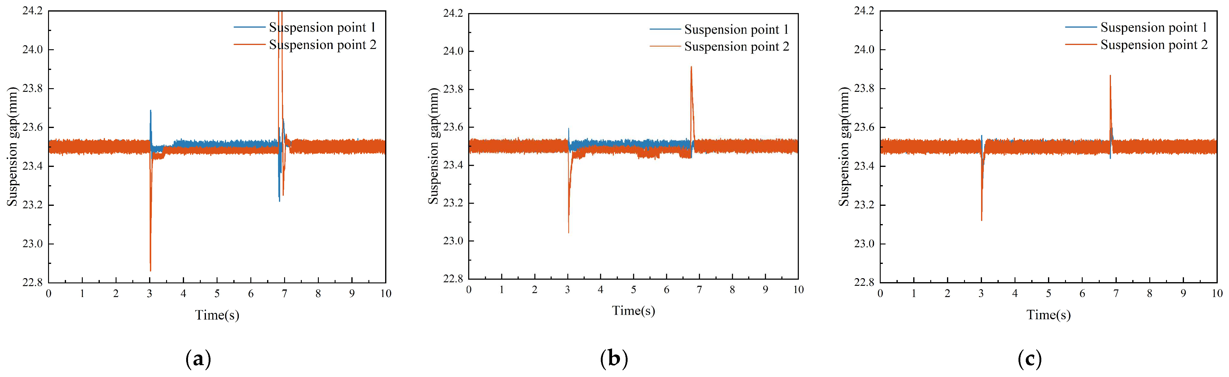
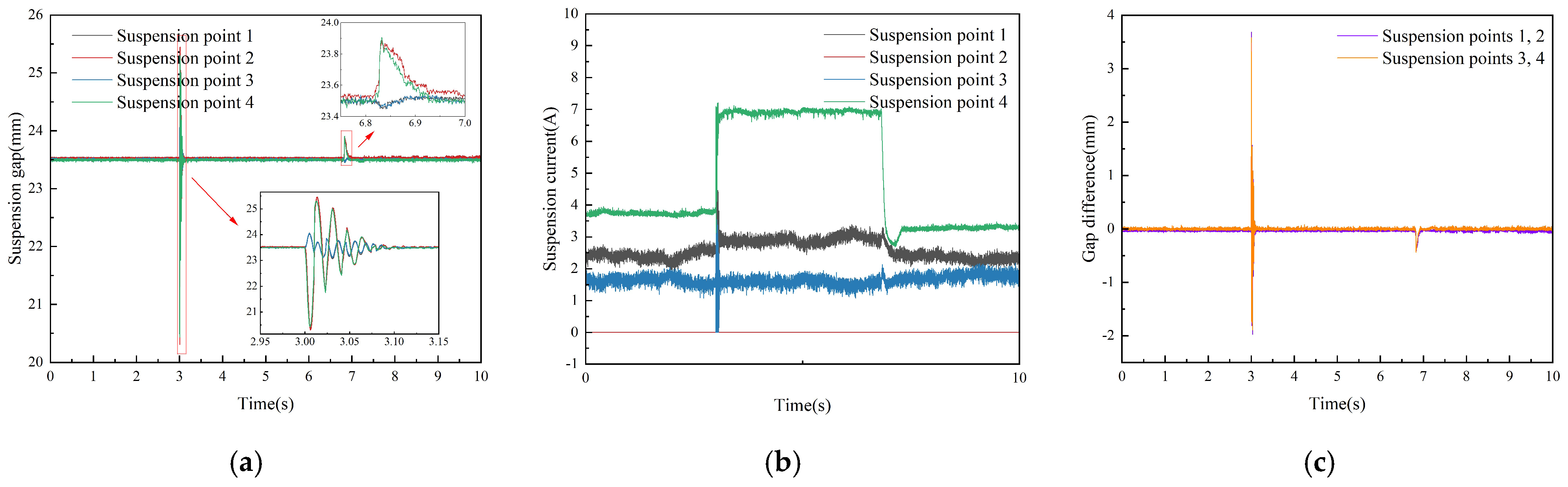
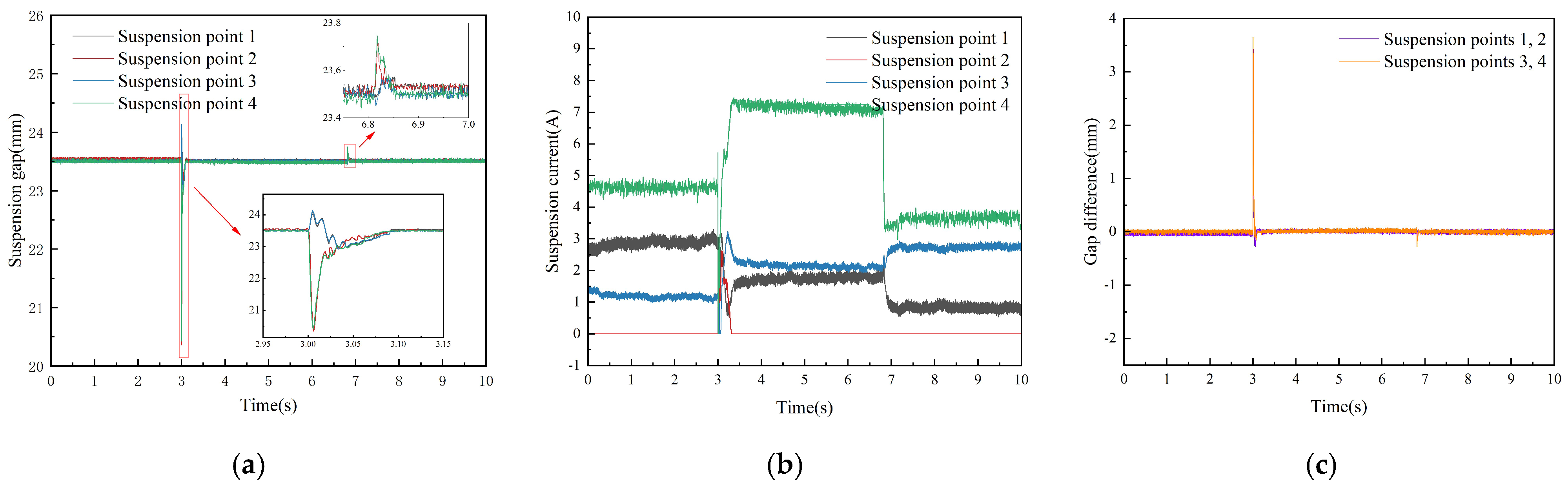
5.3. Four-Point Suspension Immunity Experiment

In this paper, to more comprehensively evaluate the control performance of ALADRCC compared to the traditional parallel independent suspension control (PID) in complex environments, a set of four-point suspension immunity experiments is designed and implemented on a multi-point hybrid suspension experimental platform. During the experiments, the parameters of the two control algorithms, ALADRCC and PID, are first parameterized separately to ensure that their respective control performances are optimized. To ensure the fairness and comparability of the experiments, this paper unifies and optimizes the core parameters of the two control strategies and records their final experimental parameters, as shown in

Table 8. Control algorithm parameters for four-point suspension immunity experiments.

Suspension Point	PID	ALADRCC
1	$\begin{array}{l}{K}_p=9\\ K_i=10\\ K_d=0.31\end{array}$	$\begin{array}{l}h=0.001\\ h_0=0.01\\ r_0=100\\ {\omega }_c=5\\ {\omega }_{0\max }=390\end{array}$$\begin{array}{l}{\omega }_{0\min }=190\\ k_{\omega }=2\\ b_0=1.5\\ c_1=80\\ c_2=0.1\end{array}$
2	$\begin{array}{l}{K}_p=4\\ K_i=10\\ K_d=0.29\end{array}$	$\begin{array}{l}h=0.001\\ h_0=0.01\\ r_0=100\\ {\omega }_c=5\\ {\omega }_{0\max }=490\end{array}$$\begin{array}{l}{\omega }_{0\min }=290\\ k_{\omega }=2\\ b_0=2.8\\ c_1=80\\ c_2=0.1\end{array}$
3	$\begin{array}{l}{K}_p=9\\ K_i=10\\ K_d=0.42\end{array}$	$\begin{array}{l}h=0.001\\ h_0=0.01\\ r_0=100\\ {\omega }_c=5\\ {\omega }_{0\max }=390\end{array}$$\begin{array}{l}{\omega }_{0\min }=190\\ k_{\omega }=2\\ b_0=1.5\\ c_1=80\\ c_2=0.1\end{array}$
4	$\begin{array}{l}{K}_p=4\\ K_i=10\\ K_d=0.11\end{array}$	$\begin{array}{l}h=0.001\\ h_0=0.01\\ r_0=100\\ {\omega }_c=5\\ {\omega }_{0\max }=490\end{array}$$\begin{array}{l}{\omega }_{0\min }=290\\ k_{\omega }=2\\ b_0=2.8\\ c_1=80\\ c_2=0.1\end{array}$

.

To ensure the reproducibility and comparability of the experimental results, the load made of rubber was selected, and the doors, windows, and ventilation system were closed during the experiment. The experimental setup is as follows: A load weighing 2 kg free-falls from a height of 0.3 m to the position of suspension point 2 at 3 s. After keeping the load for a predetermined period of time, the load is then removed. Then, the results of the four-point suspension immunity experiments under the two control algorithms, PID and ALADRCC, are recorded in the Figure 20 and Figure 21.

From the suspension gap response curves, it can be seen that, under the conventional parallel PID control, when the load is released from a high position, the amplitude of the suspension gap fluctuation is 5.144 mm, the peaks of the suspension gap fluctuation at the four suspension points are 0.528 mm, 3.193 mm, 0.564 mm, and 3.067 mm, respectively, and the suspension gap recovers to the steady state after about 92 ms. When the load is removed, the peak values of the suspension gap fluctuation at the four suspension points are 0.053 mm, 0.391 mm, 0.049 mm, and 0.409 mm, respectively, and the suspension gap recovers to the steady state after about 114 ms. With ALADRCC control, when subjected to load impact, the amplitude of suspension gap fluctuation is 3.781 mm—which is 26.49% lower compared to PID control—the peaks of suspension gap fluctuation at the four suspension points are 0.531 mm, 3.144 mm, 0.637 mm, and 3.077 mm, respectively, and the suspension gap returns to the steady state after about 89 ms—which is 3.26% faster compared to the PID control—after withdrawing the load. The peak values of suspension gap fluctuations at the four suspension points when the load is removed are 0.075 mm, 0.214 mm, 0.075 mm, and 0.249 mm, respectively, and these return to the steady state after about 53 ms, which is 53.51% faster than that of the PID control. Through the suspension current response curve, it can be observed that suspension point 2 under PID control is always unresponsive. In contrast, when subjected to shock perturbation, suspension point 2 under ALADRCC control responds immediately, and the suspension current increases with the increase and then decreases to zero after restoring the equilibrium. Hence, the perturbation adaptability of the ALADRCC is superior to that of the PID control. From the relative suspension gap difference curve, it can be learned that the peak value of the suspension gap difference between suspension point 1 and suspension point 2 under PID control is 3.682 mm, the peak value of the suspension gap difference between suspension point 3 and suspension point 4 is 3.569 mm when the disturbance is applied, the peak value of the suspension gap difference between suspension point 1 and suspension point 2 when the disturbance is withdrawn is 0.397 mm, and the peak value of the suspension gap difference between suspension point 3 and suspension point 4 is 0.402 mm. The peak suspension gap difference between suspension point 1 and suspension point 2 under ALADRCC control is 3.653 mm, the peak suspension gap difference between suspension point 3 and suspension point 4 is 3.651 mm, the peak suspension gap difference between suspension point 1 and suspension point 2 under ALADRCC control is 0.204 mm, and the peak suspension gap difference between suspension point 3 and suspension point 4 under ALADRCC control is 0.236 mm. The performance of the control algorithm for the four-point suspension immunity experiments is shown in

Table 9. Control algorithm performance for four-point suspension immunity experiments.

Performance		PID	ALADRCC
(1) Load shock	Regulation time	92 ms	89 ms
	Maximum fluctuation	5.144 mm	3.781 mm
	Steady-state current ripple	0.521 A	0.384 A
	Maximum suspension gap difference between suspension point 1 and suspension point 2	3.682 mm	3.653 mm
	Maximum suspension gap difference between suspension point 3 and suspension point 4	3.569 mm	3.651 mm
(2) Remove load	Regulation time	114 ms	53 ms
	Maximum fluctuation	0.437 mm	0.276 mm
	Steady-state current ripple	0.518 A	0.373 A
	Maximum suspension gap difference between suspension point 1 and suspension point 2	0.397 mm	0.204 mm
	Maximum suspension gap difference between suspension point 3 and suspension point 4	0.402 mm	0.236 mm

. The experimental results show that when subjected to external perturbation, ALADRCC is able to quickly adjust the suspension gap back to a stable state with a shorter adjustment time, the outputs of the four suspension points are effectively synergized, the suspension gap curves are synchronized, and the amplitude of the fluctuation of the suspension gap is significantly reduced. This demonstrates excellent robustness and overall anti-interference performance.

6. Conclusions

In this paper, ALADRCC is proposed to improve the overall anti-interference performance of a multi-point hybrid suspension system. Firstly, the mathematical models of single-point and multi-point hybrid suspension systems are established, and the coupling relationship between the multi-points is analyzed. Secondly, an ALESO with both dynamic response performance and noise suppression capability is designed, and a CCC is designed and integrated into the linear error feedback control law of ALADRC to reduce the synchronization error between neighboring suspension points effectively and improve the synchronization coordination capability of the system. Then, a simulation model is built on the MATLAB/Simulink platform, and the simulation model is simulated to improve the overall anti-jamming performance of the system. Next, a simulation model is built on the MATLAB/Simulink platform, and the simulation model is simulated to improve the overall anti-jamming performance of the system. Then, a simulation model is built on the MATLAB/Simulink platform, and the effectiveness of the designed ALESO and CCC is verified through simulation. Finally, a multi-point hybrid suspension experimental platform has been built, and experiments have proved that the multi-point hybrid suspension system under the control of the proposed ALADRCC has an excellent overall anti-interference performance. Future research will focus on reducing the complexity of parameter tuning in ALADRCC.

References

1. Tang, W.B.; Xiao, L.Y.; Wang, S.; Zhang, J.Y. Summary of Research on Levitation-guidance Modes in Maglev Rail Transportation Technology. Adv. Technol. Electr. Eng. Energy 2022, 41, 45–60. [Google Scholar]
2. Gao, T.; Yang, J.; Zhou, F.Z.; Cao, Z.H. Design and Analysis of a Permanent Magnet Electromagnetic Hybrid Levitation Control Experiment Based on COMSOL. Exp. Technol. Manag. 2024, 41, 165–174. [Google Scholar]
3. Wang, Y.G.; Yang, J.; Cui, Y.M. Characteristic Analysis of Permanent Magnet Electromagnetic Hybrid Suspension Guidance System for Maglev Train. Electr. Driv. Locomot. 2021, 6, 1–8. [Google Scholar]
4. Liang, Z.H.; Wu, H.B.; Yang, X.; Li, Q.J. Application of Fuzzy-PID Control Algorithm to Hybrid Maglev System. J. Shenyang Polytech. Univ. 2008, 1, 32–37. [Google Scholar]
5. Yang, J.; Qin, Y.; Wang, Y.Z.; Zhang, Z.L. Improved Sliding Mode Control Method for Permanent Magnet Electromagnetic Hybrid Magnetic Levitation Ball. J. Hunan Univ. Nat. Sci. 2023, 50, 200–209. [Google Scholar]
6. Hu, W.J.; Zhou, Y.H.; Zhang, Z.L.; Fujita, H. Model Predictive Control for Hybrid Levitation Systems of Maglev Trains With State Constraints. IEEE Trans. Veh. Technol. 2021, 70, 9972–9985. [Google Scholar] [CrossRef]
7. Han, W.J.; Tan, W. Tuning of Linear Active Disturbance Rejection Controllers Based on PID Tuning Rules. Control. Decis. 2021, 36, 1592–1600. [Google Scholar]
8. Song, X.J.; Li, L.Q.; Xue, W.C.; Song, K.; Xin, B. Active Disturbance Rejection Decoupling Control for Nonlinear MIMO Uncertain Systems with Application to Path Following of Self-driving Bus. Control Eng. Pract. 2023, 133, 105432. [Google Scholar] [CrossRef]
9. Wang, J.S.; Jiang, Q.L.; Luo, Y.; Liu, T.F. Active Disturbance Rejection Generalized Predictive Control for Magnetic Levitation System. J. Harbin Inst. Technol. 2022, 54, 141–150. [Google Scholar]
10. Qin, Y.; Yang, J.; Guo, H.Q.; Wang, Y.Z. Fuzzy Linear Active Disturbance Rejection Control Method for Permanent Magnet Electromagnetic Hybrid Suspension Platform. Appl. Sci. 2023, 13, 2631. [Google Scholar] [CrossRef]
11. Liu, Z.T.; Lin, W.Y.; Yu, X.H.; Rodríguez-Andina, J.J.; Gao, H.J. Approximation-Free Robust Synchronization Control for Dual-Linear-Motors-Driven Systems With Uncertainties and Disturbances. IEEE Trans. Ind. Electron. 2022, 69, 10500–10509. [Google Scholar] [CrossRef]
12. Hu, N.T.; Chen, L.Y.; Chen, C.S. Novel Cross-Coupling Position Command Shaping Controller Using H∞ in Multiaxis Motion Systems. IEEE Trans. Ind. Electron. 2022, 69, 13099–13110. [Google Scholar] [CrossRef]
13. Shang, W.W.; Xie, F.; Zhang, B.; Cong, S.; Li, Z.J. Adaptive Cross-Coupled Control of Cable-Driven Parallel Robots With Model Uncertainties. IEEE Robot. Autom. Lett. 2020, 5, 4110–4117. [Google Scholar] [CrossRef]
14. Ling, J.H.; Lu, Y.B.; Pi, D.Y.; Yin, J.D.; Zhang, W.C.; Wang, F.A.; Feng, J.W.; Zhou, C.B. A Decentralized Cooperative Control Framework for Active Steering and Active Suspension: Multi-Agent Approach. IEEE Trans. Transp. Electrif. 2022, 8, 1414–1429. [Google Scholar] [CrossRef]
15. Feng, J.W.; Liang, J.H.; Lu, Y.B.; Zhang, W.C.; Pi, D.W.; Yin, G.D.; Xu, L.W.; Peng, P.; Zhou, C.B. An Integrated Control Framework for Torque Vectoring and Active Suspension System. Chin. J. Mech. Eng. 2024, 37, 75–86. [Google Scholar] [CrossRef]
16. Li, Q.N.; Xu, D.H. Gap Cross-coupling Control for 4-Electromagnet Supported Steel Plate Magnetic Suspension System. Proc. CSEE 2010, 30, 129–134. [Google Scholar]
17. Xu, J.Q.; Lin, G.B.; Chen, C.; Rong, L.J.; Ji, W. Modeling and Control of Multi-point Levitation of Maglev Vehicle Under Loading Disturbance. J. Tongji Univ. Nat. Sci. 2020, 48, 1353–1363. [Google Scholar]
18. Wang, M.Q.; Hao, Z.Y.; He, Y.X.; Zeng, S.H.; Qi, Z.; Liu, P.F. Active Disturbance Rejection Backstepping Cross-Coupling Controller Design for a Magnetic Levitation Vehicle Suspension Frame. IEEE Trans. Transp. Electrif. 2025, 11, 4634–4644. [Google Scholar] [CrossRef]
19. Zhang, D.D.; Sun, Y.G.; Jia, N.; Sun, W. Adaptive Fuzzy Super-twisting Sliding Mode Control for the Multi-electromagnets Levitation System of Maglev Vehicles: Design and Experiments. IEEE Trans. Intell. Veh. 2024; early access. [Google Scholar]
20. Huang, X.Y.; Kang, J.S.; Ding, H.; Xia, C.; Huang, D.X.; Wang, F.X. Adjacent Cross-Coupling Control for Magnetic Levitation System With Ultra-Local Sliding Mode Algorithm. IEEE Trans. Veh. Technol. 2025, 74, 2418–2428. [Google Scholar] [CrossRef]
21. Zhao, C.; Sun, F.; Pei, W.Z.; Jin, J.J.; Xu, F.C.; Zhang, X.Y. Independent Cascade Control Method for Permanent Magnetic Levitation Platform. J. Southwest. Jiaotong Univ. 2022, 57, 618–626. [Google Scholar]
Figure 1. Structure of multi-point hybrid suspension.
Actuators 14 00312 g001
Figure 2. Dynamic model of the single-point hybrid suspension system.
Actuators 14 00312 g002
Figure 3. Dynamic model of the unilateral hybrid suspension system.
Actuators 14 00312 g003
Figure 4. Block diagram of the open-loop model of the unilateral hybrid suspension system.
Actuators 14 00312 g004
Figure 5. Block diagram of serial closed-loop control of multi-point hybrid suspension system.
Actuators 14 00312 g005
Figure 6. Current tracking simulation waveform.
Actuators 14 00312 g006
Figure 7. Block diagram of the structure of ALESO.
Actuators 14 00312 g007
Figure 8. Block diagram of the ALADRCC algorithm structure.
Actuators 14 00312 g008
Figure 9. Simulation model of single-point hybrid suspension system control.
Actuators 14 00312 g009
Figure 10. Single-point immunity simulation experiment curve. (a) Suspension gap response curve. (b) Suspension current response curve (c) ω0 response curve.
Actuators 14 00312 g010
Figure 11. Simulation model for control of multi-point hybrid suspension system.
Actuators 14 00312 g011
Figure 12. Simulation experiment curve for c 1 = 0 ,   c 2 = 0 . (a) Suspension gap response curve. (b) Suspension current response curve. (c) Suspension gap difference curve.
Actuators 14 00312 g012
Figure 13. Simulation experiment curve for c 1 = 100 ,   c 2 = 0.1 . (a) Suspension gap response curve. (b) Suspension current response curve. (c) Suspension gap difference curve.
Actuators 14 00312 g013
Figure 14. Simulation experiment curve for c 1 = 1000 ,   c 2 = 0.1 . (a) Suspension gap response curve. (b) Suspension current response curve. (c) Suspension gap difference curve.
Actuators 14 00312 g014
Figure 15. Multi-point hybrid suspension experiment platform.
Actuators 14 00312 g015
Figure 16. Single-point immunity experiment curve. (a) Suspension gap response curve. (b) Suspension current response curve. (c) ω 0 response curve.
Actuators 14 00312 g016
Figure 17. Gap response curve of the unilateral immunity experiment. (a) PID. (b) ALADRC. (c) ALADRCC.
Actuators 14 00312 g017
Figure 18. Current response curve of the unilateral immunity experiment. (a) PID. (b) ALADRC. (c) ALADRCC.
Actuators 14 00312 g018
Figure 19. Suspension gap difference curve of the unilateral immunity experiment. (a) PID. (b) ALADRC. (c) ALADRCC.
Actuators 14 00312 g019
Figure 20. PID algorithm. (a) Suspension gap response curve. (b) Suspension current response curve. (c) Suspension gap difference curve.
Actuators 14 00312 g020
Figure 21. ALADRCC algorithm. (a) Suspension gap response curve. (b) Suspension current response curve. (c) Suspension gap difference curve.
Actuators 14 00312 g021