Research on Sensorless Control Strategy of High-Speed Submersible Permanent Magnet Synchronous Motor

Abstract

The application fields of high-speed submersible permanent magnet synchronous motors (PMSM) are constantly expanding. Especially in high-risk and complex environments such as oil exploration, offshore oil exploitation, and deep well operation, the reliability, stability, and efficiency of motor drive systems are more and more prominent. The submersible motor is greatly affected by load disturbance, pressure change, and external oil flow, and the traditional method may not perform well in complex disturbance problems. Therefore, a three-order adaptive nonlinear extended state observer is proposed to collect the input and output information of the system in real time, and estimate the motor speed, position, and total disturbance. A linear feedback control law is designed to eliminate the disturbance. The superiority of the proposed algorithm under complex operating conditions is verified by the Simulink model and experiments, which provide a theoretical basis for the control of submersible motors.

1. Introduction

High-speed submersible permanent magnet synchronous motor (PMSM), as a new type of highly efficient driving equipment, is widely used in submersible electric pump (ESP) systems in the oil and gas industry. In recent years, with the continuous increase in the demand for efficient and low-energy-consuming equipment in the energy industry, high-speed submersible permanent magnet synchronous motors, with their outstanding power density, high efficiency, and stability, have become one of the important equipment for deep well operations and oil and gas exploration. Permanent magnet synchronous motors feature high power factor, low energy consumption, and excellent dynamic response characteristics, and perform particularly well in high-speed operation and harsh underground environments. With the continuous advancement of microprocessor technology, intelligent algorithms, and motor control technology, the application fields of high-speed submersible permanent magnet synchronous motors are also constantly expanding. Especially in high-risk and complex environments such as oil exploration, offshore oil extraction, and deep well operations, the requirements for the reliability, stability, and efficiency of motor drive systems have become increasingly prominent.

Most traditional submersible motors adopt control methods equipped with position sensors. However, due to the extremely harsh working environment, these mechanical position sensors are prone to be affected by factors such as high temperature, high pressure, and moisture, which can lead to a decline in system control performance or even failure [1,2]. Therefore, position-free control technology has become a hot topic in the current research of high-speed submersible permanent magnet synchronous motors [3,4,5,6,7,8]. The core advantage of position-free control technology lies in eliminating mechanical sensors, thereby reducing system complexity and cost, and effectively enhancing motor reliability. By precisely establishing a mathematical model and applying control algorithms, the position and speed of the motor rotor can be estimated in real time, achieving precise control of the motor [9,10,11,12,13,14,15]. In recent years, position sensorless vector Control technology (Field Oriented Control, FOC) has been widely applied in the field of motor control. This technology achieves precise regulation of stator current to enable effective control over motor magnetic fields, thereby enhancing operational efficiency and dynamic response capabilities, particularly excelling under high-load and high-speed operating conditions. With the continuous advancement of motor control technologies, PMSM control methodologies have undergone iterative optimization. Researchers have conducted in-depth investigations into high-efficiency control strategies to further improve system stability and response speed. Field-Oriented Control (FOC), initially proposed by Dr. Hasse in the mid-20th century, derives its theoretical foundation from magnetic field orientation principles. Subsequent refinements by researchers such as Blaschke facilitated its evolution into a mainstream control method for PMSMs and other AC motors. FOC has gained extensive adoption in sensorless control applications due to its superior dynamic and static performance. The implementation of this technology relies on accurate rotor position and speed estimation to ensure the effectiveness of closed-loop control systems [16,17,18,19,20,21].

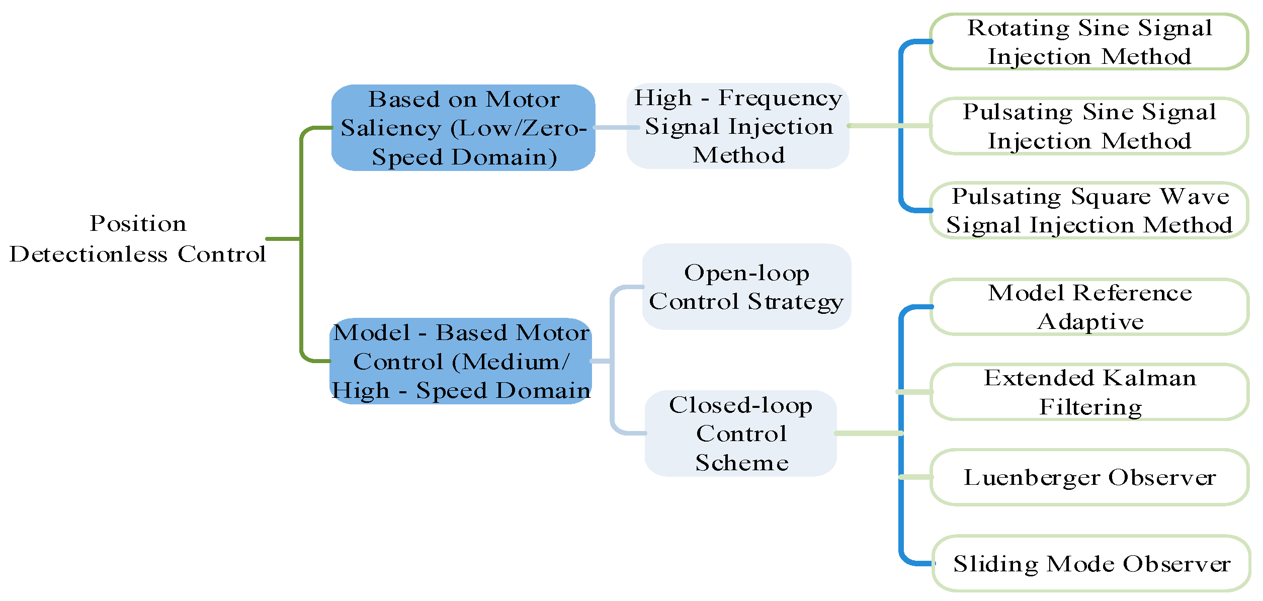
In the research on sensorless control technologies, according to the different speed ranges of motor operation, the technology can be categorized into the salient-pole method and the motor model observation method, as shown in Figure 1. The salient-pole method is primarily applied in the zero-speed and low-speed operation stages. During this phase, the counter electromotive force (EMF) signal is too weak to be directly used for rotor position estimation. Therefore, this method leverages the inherent salient-pole effect of the motor, that is, the asymmetry characteristic of the quadrature and direct axis inductances, to extract components containing position information from the stator current signal, thereby achieving sensorless position detection. The motor model observation method is suitable for medium- and high-speed operation regions. When the motor enters this operating state, the counter EMF signal becomes significant and easy to measure. By constructing a mathematical model, the rotor position and speed can be calculated based on the variation trend of the counter EMF, thus providing precise feedback for motor control and enhancing the dynamic performance of the system.

Submerged oil motors are highly susceptible to load disturbances, pressure variations, and external oil flow. Traditional control methods may be less effective in handling complex disturbance issues. In Active Disturbance Rejection Control (ADRC), the Extended State Observer (ESO) is central. It precisely estimates various system disturbances in real time by collecting system input and output information [22,23]. Then, it quickly generates corresponding compensation signals to enhance system robustness and response speed. ADRC aims to effectively handle various internal and external system interferences and fluctuations, achieving superior control results. Its core concept is the ESO, which assesses and counteracts uncertainties and external factors in the control system. By real-time monitoring and analysis of disturbance characteristics, the ESO can monitor disturbances and their impact on system behavior, adjusting control signals to maintain system stability and performance even with disturbances. Notably, this method does not rely on detailed mathematical model descriptions. Instead, it adaptively learns and compensates based on data collected during actual operation, making it a promising control strategy for submerged oil motors in complex working conditions. Lian Chaojie et al. [24] designed a third-order nonlinear ADRC position controller for a double-cylinder system to realize real-time estimation and active compensation of internal and external system disturbances. Liu Yuxing et al. [25] proposed a hybrid control method combining fuzzy control and linear ADRC for direct-drive permanent magnet synchronous wind power generation systems. This method addressed issues of variable wind speed, nonlinearity, and strong disturbances, enhancing the system’s anti-disturbance ability and robustness. Nguyen et al. [26] presented an ADRCBF method based on dynamic fuzzy adjustment. It effectively reduced vehicle vibration and improved the suspension system’s adaptability and control accuracy across different road conditions.

Based on the active disturbance rejection control theory, the working mechanisms of the flux chain-locked loop and the extended state observer were studied. Their deficiencies were analyzed from the perspective of errors. The innovation point of this paper lies in the introduction of the adaptive nonlinear Extended State Observer (ANLESO). This ANLESO replaced the magnetic chain-locked phase loop and estimated the total disturbance inside and outside the system. These estimated interferences are then regulated in the speed adjustment component. The purpose of this method is to enhance the robustness of the system and improve the performance indicators of dynamic response. In the final stage of the research, a simulation model was established on the Simulink platform. The proposed strategy is applied to various working conditions to verify its effectiveness.

2. Analysis of the Traditional ADRC Principle

2.1. The Principle of ADRC Control

In the realm of ADRC, a novel methodology is employed for processing input signals and mitigating system disturbances. Initially, the Tracking Differentiator (TD) is utilized to optimize the system input, meticulously designing the transition process of the input signal to ensure precise tracking of the desired target values by the system. Subsequently, the Extended State Observer (ESO) incorporates supplementary state variables, treating internal and external disturbances as an aggregated disturbance source and enabling effective estimation of these disturbances. The estimates derived from this process are fed back into the controller, which employs a Nonlinear State Error Feedback (NLSEF) mechanism to adjust the control variables based on the estimation results, thereby effectively attenuating the impact of the disturbances. This paradigm enhances the system’s robustness and precision in following the desired trajectories, marking a significant advancement in control theory and its practical applications.

2.2. The Principle of Nonlinear ADRC

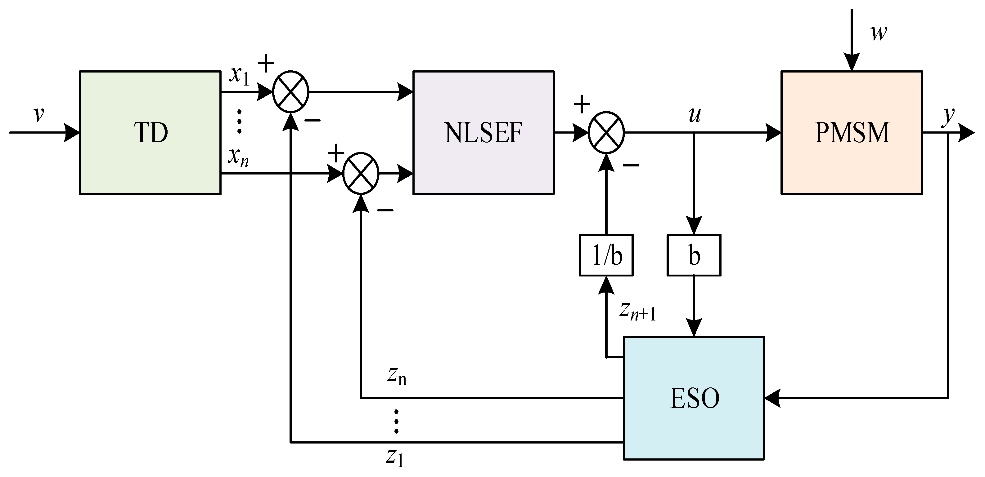
As shown in Figure 2, the ADRC controller comprises three key components: the TD for managing transients, the ESO for observing system states, and the NLSEF for compensating errors. In this diagram, v denotes the system input, which, after passing through the TD, generates tracking signals and derivatives. The system output y and control input u are fed into the ESO to estimate state variables and comprehensive disturbances. The NLSEF then calculates control adjustments to counteract these disturbances, with 1/b serving as the feedforward compensation gain. Finally, the discrepancy between TD and ESO outputs is processed by the NLSEF, combined with feedforward compensation, to achieve precise system control.

As can be seen, ADRC is applicable to nonlinear control systems with unknown disturbances, and its corresponding control equation is as follows:

$$\left\{\begin{array}{l}{x}^{(n)}=f(x,\dot{x},\dots ,x^{(n-1)},t)+w(t)+bu\\ y=x(t)\end{array}\right.,$$

(1)

From Equation (1), it is evident that there exists an undefined function $f(x,\dot{x},\dots ,x^{(n-1)},t)$. In addition, the system is subject to uncertain external disturbances w(t). The control action u of the system itself is also a key factor. Moreover, the gain parameter b plays a significant role. Finally, the performance of the entire system can be evaluated through the quantifiable output index x(t).

2.2.1. Tracking Differentiator

When applying a PID control strategy, system overshoot is almost inevitable [27]. In contrast, the transient dynamics approach enables step inputs to smoothly approach target values at a predetermined rate, essentially initiating a transitional process in advance. This method first identifies ideal set points and their associated differential information from data that may contain discontinuities or noise. It then provides a smooth variation path for the original signal, enabling it to rapidly and oscillation-free follow the given target. This improves the system’s response characteristics.

Nevertheless, although TD can balance rapid response and overshoot reduction, its inherent gradual adjustment mechanism may exhibit limitations in the face of high-frequency varying input signals. It might even lead to performance degradation or failure.

The differential signal of TD can be approximately expressed as follows [28]:

$$\dot{v}(t)\approx {\displaystyle \frac{v(t-{\tau }_2)-v(t-{\tau }_1)}{{\tau }_1-{\tau }_2}}$$

(2)

where ${\tau }_1$, ${\tau }_2$ is the differential step size and there is $0\le {\tau }_1\le {\tau }_2$. The transfer function is as follows:

$$G(s)={\displaystyle \frac{r^2}{s^2+2rs+r^2}}$$

(3)

where r is the speed factor, and the magnitude of the change controls the signal tracking speed.

Take the second-order system as an example:

$$\left\{\begin{array}{l}{\dot{x}}_1=x_2\\ {\dot{x}}_2=u,\left|u\right|\le r\end{array}\right.$$

(4)

Fast optimal control can be expressed as

$$\left\{\begin{array}{l}{\dot{x}}_1=x_2\\ {\dot{x}}_2=-r\cdot \mathrm{sgn}[x_1-v(t)+x_2\left|x_2\right|/2r]\end{array}\right.$$

(5)

where when $\left|{\ddot{x}}_1\right|\le r$ is satisfied, the system can efficiently track the specified signal v(t), and its tracking speed increases with the increase of the parameter r value. Based on the above discussion, the discrete form of the TD system can be expressed as

$$\left\{\begin{array}{l}{x}_1(k+1)=x_1(k)+h{x}_1(k)\\ x_2(k+1)=x_2(k)+fhan(x_1(k)-x(k),x_2(k),r,h)\end{array}\right.$$

(6)

where x(k) represents the value of the given signal at a specific time point; x₁(k) indicates the specific value of the tracking signal at the same moment; x₂(k) refers to the differential estimation of the measurement result of the signal at that moment; h is the time interval adopted in the integration process, s; fhan is the Fastest Control Synthesis Function in the Tracking Differentiator.

The expression equation of TD is as follows:

$$\left\{\begin{array}{l}d=rh\\ d_0=hd\\ y=x_1-v+h{x}_2\\ a_0=\sqrt{d^2+8a\left|y\right|}\\ a=\left\{\begin{array}{l}{x}_2+{\displaystyle \frac{(a_0-d)}{2}}sign(y),\left|y\right|>d_0\\ x_2+{\displaystyle \frac{y}{h}}, \left|y\right|\le d_0\end{array}\right.\\ fhan=-\left\{\begin{array}{l}rsign(a), \left|a\right|>d\\ r{\displaystyle \frac{a}{d}}, \left|a\right|\le d\end{array}\right.\end{array}\right.$$

(7)

where d represents the adjustment range of the control error; d₀ is the limit value for error correction; y is the trajectory error; a₀ is the reference value for error correction; a is the error signal that has undergone nonlinear adjustment; fhan is the control signal after nonlinear processing.

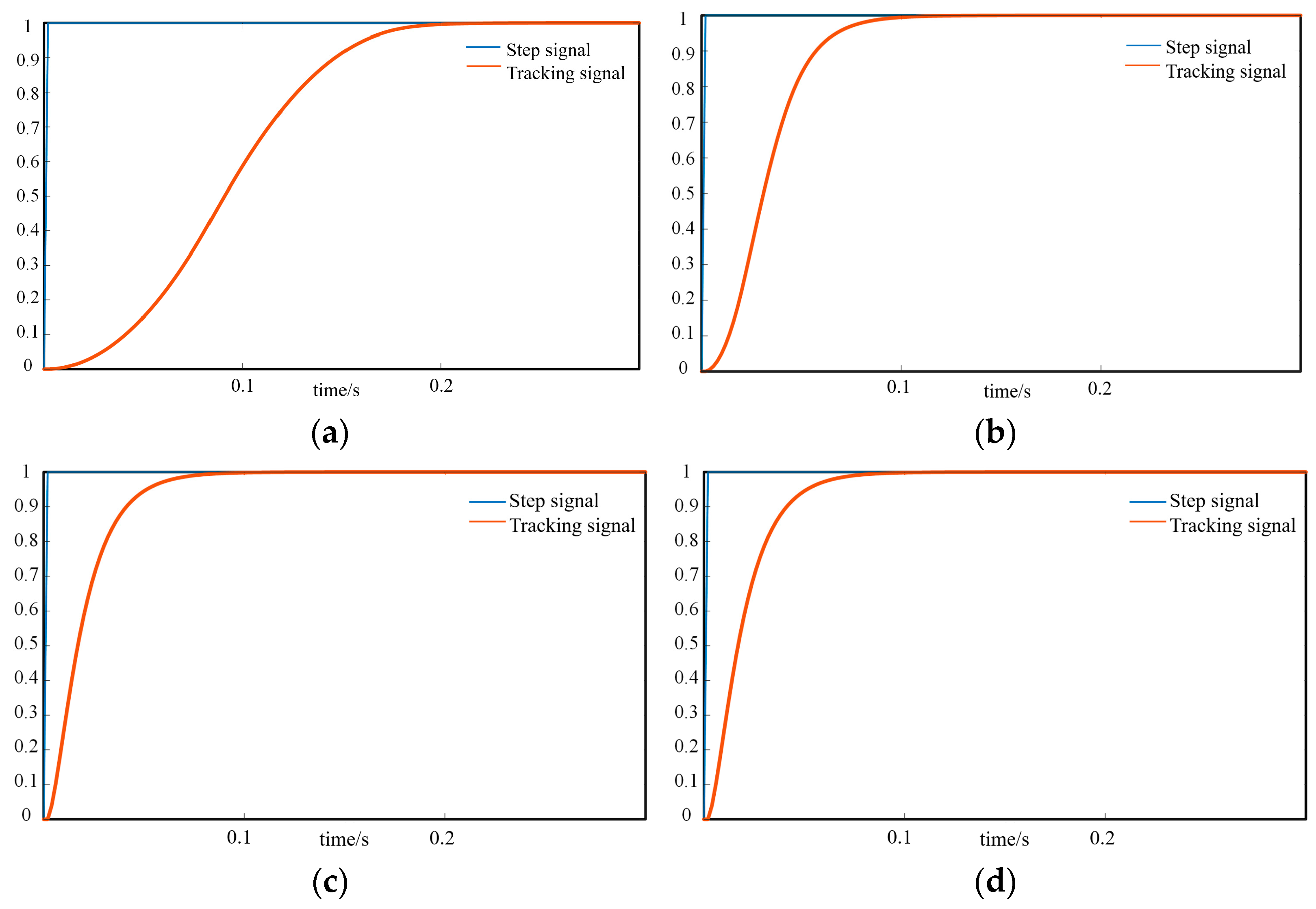
TD can generate tracking signals quickly and accurately. It is crucial to select the speed factor r reasonably. When the input v is the unit step function, the situations where the r values are 100, 1000, 10,000, and 50,000 were tested, respectively. The simulation results are detailed in Figure 3.

As shown in Figure 3, with the increase of the r value, the time difference between the tracking signal and the step signal becomes smaller and smaller. However, when the r value is too large, it tends to have a step response characteristic. At this time, the original design intention of the transition process is difficult to achieve, resulting in TD being unable to generate the tracking signal after the transition and also affecting the subsequent estimation of state variables. Therefore, various situations need to be comprehensively considered. It is necessary to generate good transition signals while maintaining the good dynamic characteristics of the entire control system.

2.2.2. Expanded State Observer

ESO, as the second link in ADRC and the most core part, the control effect of ADRC mostly depends on the design of ESO. The main function of ESO is to estimate the total disturbances inside and outside the system based on the input and output information of the system, so as to compensate for the subsequent links.

It is particularly worth noting that in practical operation, compared with traditional observers, ESO has a lower reliance on the mathematical model of the motor, does not require precise measurement of external interference, and improves the robustness of the entire control system.

Taking the second-order control system as an example, the nonlinear expanded state observer (NLESO) is designed:

$$\left\{\begin{array}{l}{\dot{x}}_1=x_2\\ {\dot{x}}_2=f(x_1,x_2,w(t),t)+b_{0}u\\ y=x_1\end{array}\right.$$

(8)

Equation (8) is its state space equation. The internal and external disturbances experienced by the system are regarded as an overall disturbance and incorporated as a new state variable. In this way, the original system can be re-expressed as

$$\left\{\begin{array}{l}{\dot{x}}_1=x_2\\ {\dot{x}}_2=x_3+b_{0}u\\ {\dot{x}}_3=w_0(t)\\ y=x_1\end{array}\right.$$

(9)

The resulting NLESO is

$$\left\{\begin{array}{l}e=z_1-y\\ {\dot{z}}_1=z_2-{\beta }_{01}fal(e,{\alpha }_1,\delta )\\ {\dot{z}}_2=z_3-{\beta }_{02}fal(e,{\alpha }_2,\delta )+b_{0}u\\ {\dot{z}}_3=-{\beta }_{03}fal(e,{\alpha }_3,\delta )\end{array}\right.$$

(10)

where e represents the observation error; Z₁, Z₂ is the observed value of the position and velocity of the system; Z₃ represents the total observed values of internal and external disturbances of the system; δ is used to divide the linear part and the length of the nonlinear interval; β₀₁, β₀₂, β₀₃ is defined as the gain parameter of the observer; α is a power, used to adjust the characteristics of the function within different error ranges.

Nonlinear functions fal() satisfy:

$$fal(e,\alpha ,\delta )=\left\{\begin{array}{l}{\displaystyle \frac{e}{{\delta }^{\alpha -1}}},\begin{array}{ll}& \left|e\right|\le \delta \end{array}\\ {\left|e\right|}^{\alpha }sign(e),\begin{array}{ll}& \left|e\right|>\delta \end{array}\end{array}\right.$$

(11)

2.2.3. Nonlinear State Error Feedback

When the error is large, NLSEF adopts a lower gain to reduce the systematic error. When the error is small, a higher gain promotes the system to respond quickly to the change of the given value. There are two common methods for NLSEF, namely:

$$u_0={\beta }_{11}fal(e_1,{\alpha }_1,\delta )+{\beta }_{22}fal(e_2,{\alpha }_2,\delta )$$

(12)

$$u_0=fhan(e_1,c{e}_2,r,h_1)$$

(13)

Formula (12) adjusts the feedback quantity by combining different coefficients β₁₁, β₂₂ with the nonlinear function fal based on different errors e₁, e₂, power coefficients α₁, α_2, and threshold δ; Formula (13) uses the fhan function to implement nonlinear error feedback based on error e₁, the rate of change of error e₁ ce₂, and parameters r and h₁, in order to adapt to different states of the system.

For $fhan(e_1,c{e}_2,r,h_1)$, there are the following expression forms:

$$\left\{\begin{array}{l}d=r{h_1}^2,a_0=c{e}_2,y=x_1+a_0\\ a_1=\sqrt{d^2+8d\left|y\right|}\\ a_2=a_0+{\displaystyle \frac{sign(y)\cdot (a_1-d)}{2}}\\ S_y={\displaystyle \frac{[sign(y+d)-sign(y-d)]}{2}}\\ a=(a_0+y-a_2)S_y+a_2\\ S_a={\displaystyle \frac{[sign(a+d)-sign(a-d)]}{2}}\\ fhan=-r[{\displaystyle \frac{a}{d}}-sign(a)]S_a-rsign(a)\end{array}\right.$$

(14)

where d represents the control error; y is the trajectory error; a₁ is the parameter for estimating the error range; a₂ is the error adjustment parameter; a is the core error adjustment amount; sign is a symbolic function; S_a is the sign correction amount of error a; S_y is the sign correction of the error y.

It can be understood from the description that the operation process of the nonlinear ADRC controller includes: Firstly, after the given signal v is processed by TD, a smooth input signal and the corresponding differential value x are generated; Then, ESO is utilized to estimate all the disturbances inside and outside the system and regard them as an overall disturbance; Finally, through the NLSEF mechanism, the above-mentioned total disturbance is combined with the nonlinear state of the system for feedback control, so as to achieve the effect of suppressing interference. At the same time, it ensures that the system will not have overmodulation throughout the process.

2.3. The Principle of Linear ADRC

In the previous chapter, the design and implementation of a nonlinear ADRC controller were discussed. Although this controller has demonstrated its unique advantages, it faces the problem of parameter calibration in practical applications. Even though the parameter range can be roughly defined by means such as time scale setting, the operation is still quite challenging and poses high requirements for the performance of the processor.

To solve this series of problems, Professor Gao Zhiqiang innovatively proposed an improved version of Active Disturbance Rejection Control (LADRC) [29,30]. This new type of controller not only simplifies the structure, but also makes parameter adjustment more convenient. It is also composed of three core modules. However, compared with the traditional nonlinear ADRC, the biggest difference lies in converting the originally complex nonlinearity into a more intuitive and understandable linear relationship.

2.3.1. Linear Tracking-Differentiator (LTD)

In the LTD method, a relatively simple linear function fh = −r²e − 2rx₂ is adopted to approximate the complex nonlinear relationship fhan(), where r = w_c (here w_c refers to the bandwidth parameter) is inversely proportional to the response speed of the system. The specific expression form of this method is [31]:

$$\left\{\begin{array}{l}{\dot{x}}_1=x_2\\ {\dot{x}}_2=-r^2[x_1-v(t)]-2r{x}_2\end{array}\right.$$

(15)

Its discrete expression is

$$\left\{\begin{array}{l}e(k)=x_1(k)-v(k)\\ x_1(k+1)=x_1(k)+h{x}_2(k)\\ x_2(k+1)=x_2(k)+hfh\\ fh=-r^{2}e(k)-2r{x}_2(k)\end{array}\right.$$

(16)

where fh represents the output of the LTD.

2.3.2. Linear Extended State Observer (LESO)

A linearized LESO can be obtained from the NLESO by replacing the nonlinear fal function with a simple error term e, thereby eliminating the need for numerous tuning parameters.

$$\left\{\begin{array}{l}e=z_1-y\\ {\dot{z}}_1=z_2-{\beta }_{01}e\\ {\dot{z}}_2=z_3-{\beta }_{02}e+b_{0}u\\ {\dot{z}}_3=-{\beta }_{03}e\end{array}\right.$$

(17)

Through the aforementioned formulation, the LESO replaces the nonlinear function fal with the error term e compared to the NLESO, consequently requiring significantly fewer parameter adjustments and exhibiting reduced complexity relative to its nonlinear counterpart.

2.3.3. Linear State Error Feedback (LSEF)

Upon obtaining the error signal, a linear combination is performed:

$$\left\{\begin{array}{l}{e}_1=x_1-z_1\\ e_2=x_2-z_2\\ u_0={\beta }_{11}{e}_1+{\beta }_{22}{e}_2\end{array}\right.$$

(18)

Based on the following control law, the estimated disturbance value from the LESO is fed back to cancel the total disturbance and maintain system stability:

$$u=u_0-{\displaystyle \frac{z_3}{b_0}}$$

(19)

$$\left\{\begin{array}{l}LTD\left\{\begin{array}{l}{\dot{x}}_1=x_2\\ {\dot{x}}_2=-r^2[x_1-v(t)]-2r{x}_2\end{array}\right.\\ LESO\left\{\begin{array}{l}e=z_1-y\\ {\dot{z}}_1=z_2-{\beta }_{01}e\\ {\dot{z}}_2=z_3-{\beta }_{02}e+b_{0}u\\ {\dot{z}}_3=-{\beta }_{03}e\end{array}\right.\\ LSEF\left\{\begin{array}{l}{e}_1=x_1-z_1\\ e_2=x_2-z_2\\ u_0={\beta }_{11}{e}_1+{\beta }_{22}{e}_2\\ u=u_0-{\displaystyle \frac{z_3}{b_0}}\end{array}\right.\end{array}\right.$$

(20)

In summary, the mathematical formulation of conventional LADRC can be derived as shown in Equation (20).

As evidenced by Equation (20), compared to ADRC, LADRC simplifies the system architecture while preserving its inherent advantages by converting the nonlinear functions in ADRC into linear forms. This transformation significantly reduces the technical barriers associated with parameter tuning. Although this conversion may marginally compromise the controller’s operational precision, the implementation simplicity has led to the widespread adoption of LADRC in numerous practical applications [32,33].

3. Adaptive Nonlinear ADRC Design

3.1. Error Analysis of Traditional Flux-Linkage Phase-Locked Loop

Figure 4 illustrates the fundamental principle of the flux-linkage PLL. The angular error calculated from the flux linkage is converted into speed and phase outputs through parameter adjustment. The key advantage of this technique lies in its transformation of speed estimation into a closed-loop control system, thereby effectively eliminating the need for direct differentiation operations.

Taking the flux-observer-based PLL as an example [34]:

$$\left\{\begin{array}{l}{e}_{\alpha }=-{\omega }_e{\psi }_{f}sin{\theta }_e\\ e_{\beta }={\omega }_e{\psi }_{f}cos{\theta }_e\end{array}\right.$$

(21)

$$\left\{\begin{array}{l}\eta ({\widehat{x}}_1)={\psi }_f\cos {\theta }_e\\ \eta ({\widehat{x}}_2)={\psi }_f\sin {\theta }_e\end{array}\right.$$

(22)

where $\eta ({\widehat{x}}_1)$, $\eta ({\widehat{x}}_2)$ are the flux linkage under the $\alpha \beta$-axis, Wb, respectively.

The calculation method for the angular error in traditional flux-linkage PLLs is as follows:

$$\begin{array}{l}\Delta {\theta }_e=\eta ({\widehat{x}}_2)\cos {\widehat{\theta }}_e-\eta ({\widehat{x}}_1)\sin {\widehat{\theta }}_e\\ ={\psi }_f(\sin {\theta }_e\cos {\widehat{\theta }}_e-\sin {\widehat{\theta }}_e\cos {\theta }_e)\\ ={\psi }_f\sin ({\theta }_e-{\widehat{\theta }}_e)\\ \approx {\theta }_e-{\widehat{\theta }}_e\end{array}$$

(23)

The angular error is processed through a PI to obtain the angular velocity w_e, expressed as:

$${\omega }_e=k_p\cdot \Delta {\theta }_e+{\displaystyle \int k_i\cdot }\Delta {\theta }_e$$

(24)

From the figure, the transfer function of the flux-linkage PLL can be derived as:

$$G_{PLL}(s)={\displaystyle \frac{{\widehat{\theta }}_e}{{\theta }_e}}={\displaystyle \frac{k_{p}s+k_i}{s^2+k_{p}s+k_i}}$$

(25)

The phase error function of the flux-linkage PLL is given by:

$$G_{PLL}(s)={\displaystyle \frac{{\theta }_e-{\widehat{\theta }}_e}{{\theta }_e}}={\displaystyle \frac{s^2}{s^2+k_{p}s+k_i}}$$

(26)

Under frequency ramp input conditions, the steady-state phase error of the flux-linkage PLL method can be calculated as follows:

$$\Delta {\theta }_{PLL}(s)=\underset{s\to 0}{\lim }{\displaystyle \frac{s^2}{s^2+k_{p}s+k_i}}\cdot {\displaystyle \frac{n}{s^3}}\cdot s={\displaystyle \frac{n}{k_i}}$$

(27)

where n represents the gain coefficient of the frequency ramp.

As can be seen from Equation (27), the flux-linkage PLL method may exhibit certain limitations in achieving high-precision estimation when the input signal frequency undergoes ramp changes (i.e., during acceleration/deceleration variations). Specifically, during linear frequency variations, the conventional flux-linkage PLL approach may encounter difficulties in accurately tracking the true system position information.

3.2. Error Analysis of Third-Order Linear Extended State Observer

To enhance the dynamic response characteristics of permanent magnet synchronous motor (PMSM) drive systems, a mechanical dynamics-based LESO [35] method has been introduced. This approach enables precise description of the motor’s dynamic behavior through dedicated formulations.

$$\left\{\begin{array}{l}J{\displaystyle \frac{d{\omega }_e}{dt}}=T_e-T_L-B{\omega }_e\\ T_e={\displaystyle \frac{3P_n{\psi }_f}{2}}{i}_q\end{array}\right.$$

(28)

where J is the rotational inertia of the control motor, kg-m²; T_L is the load torque of the controlled motor, N-m; B is the viscous damping coefficient, N·m·s/rad.

By transforming Equation (28), we obtain

$${\dot{\omega }}_e=a\cdot i_q-a_1{T}_L-a_2{\omega }_e$$

(29)

where $a=3P_n{\psi }_f/2J$; $a_1=1/J$; $a_2=B/J$.

When motor parameter perturbations are considered, the above equation can be expressed as

$${\dot{\omega }}_e=\left(a+\Delta a\right)\cdot i_q-\left(a_1+\Delta a_1\right)T_L-\left(a_2+\Delta a_2\right){\omega }_e$$

(30)

where $\Delta a$, $\Delta a_1$ and $\Delta a_2$ are the perturbation terms due to changes in the motor parameters such as $a$, $a_1$ and $a_2$, respectively, and can therefore be written as

$$\left\{\begin{array}{l}{\dot{\theta }}_e={\omega }_e\\ {\dot{\omega }}_e=a\cdot i_q+f\end{array}\right.$$

(31)

In the above equation, f covers both the known parts of the system and the unknown disturbances, such as changes in load torque, viscous friction effects, and disturbances due to q-axis currents. All these elements fulfill the requirements of Lipschitz’s boundedness.

Based on the above analysis, the mathematical expression for a third-order LESO is shown below:

$$\left\{\begin{array}{l}e={\theta }_e-{\widehat{\theta }}_e\\ {\dot{\theta }}_e={\omega }_e+{\beta }_{1}e\\ {\dot{\omega }}_e=a{i}_q+f_{11}+{\beta }_{2}e\\ {\dot{f}}_{11}={\beta }_{3}e\end{array}\right.$$

(32)

where f₁₁ is the observed perturbation; ${\beta }_1$, ${\beta }_2$, and ${\beta }_3$ are the gain parameters of the third-order LESO.

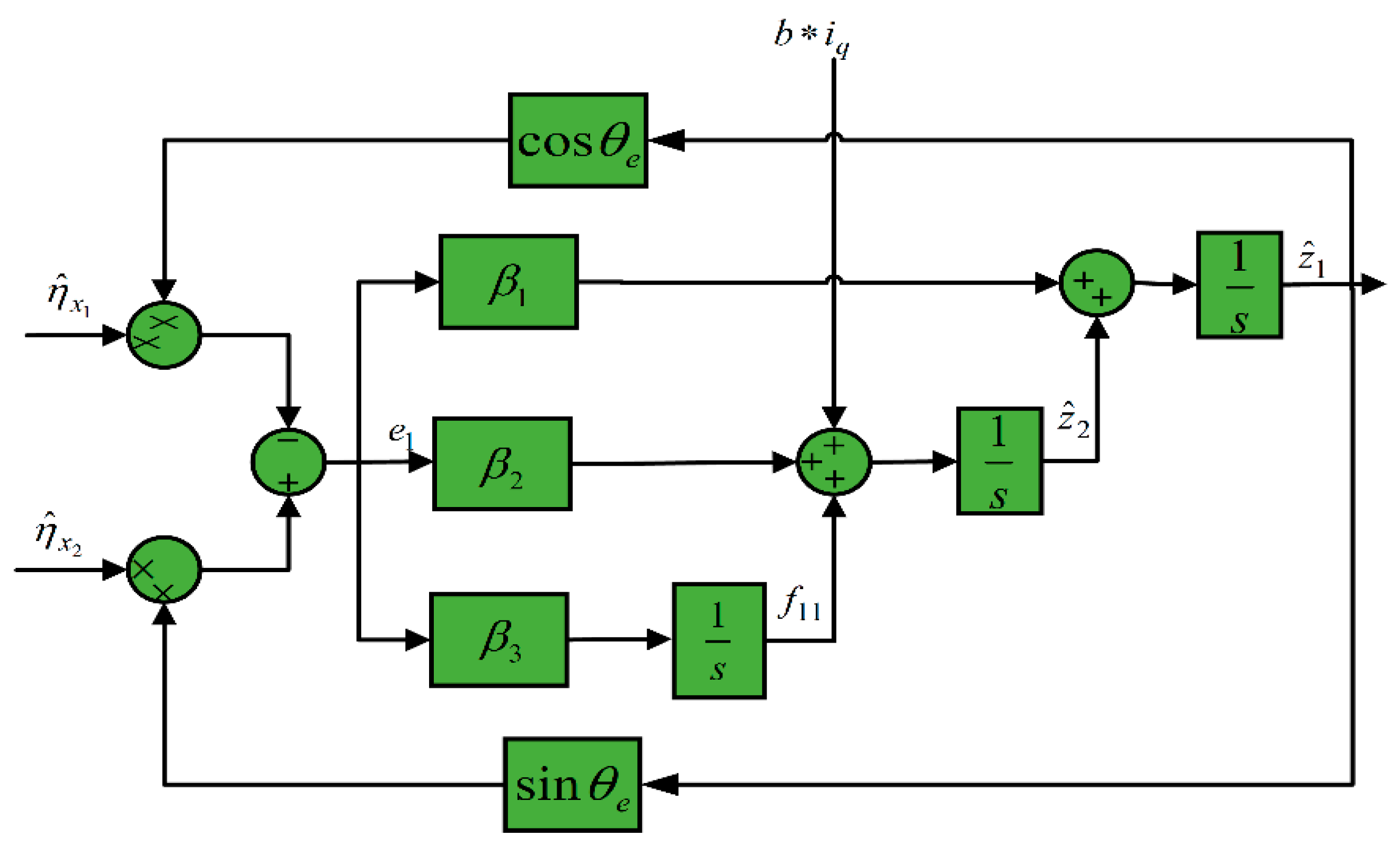
Figure 5 presents the block diagram of the third-order LESO, from which the transfer function expression of its input phase error can be derived:

$$G_{LESO}(s)={\displaystyle \frac{{\theta }_e-{\widehat{\theta }}_e}{{\theta }_e}}={\displaystyle \frac{s^3}{s^3+{\beta }_1{s}^2+{\beta }_{2}s+{\beta }_3}}$$

(33)

When the motor is accelerating and decelerating, the phase error of the third-order LESO can be calculated as follows:

$$\Delta {\theta }_{ess}^{LESO}(s)=\underset{s\to 0}{\lim }{\displaystyle \frac{s^3}{s^3+{\beta }_1{s}^2+{\beta }_{2}s+{\beta }_3}}\cdot {\displaystyle \frac{n}{s^3}}\cdot s=0$$

(34)

From Equation (32), it can be seen that under appropriate parameter adjustment, the third-order LESO can effectively track the input signal frequency changes and observe the speed and position information with high accuracy.

The derivation of the error equation for the third-order LESO is as follows:

$$\left\{\begin{array}{l}{\dot{e}}_1=e_2-{\beta }_1{e}_1\\ {\dot{e}}_2=e_3-{\beta }_2{e}_1\\ {\dot{e}}_3=h-{\beta }_3{e}_1\end{array}\right.$$

(35)

where h is a constant, and e₃ is the error correction term; e₂ and e₃ represent the speed estimation error and the total disturbance estimation error, respectively.

Also:

$$\left\{\begin{array}{l}{e}_2={\omega }_e-{\widehat{\omega }}_e\\ e_3=z-\widehat{z}\end{array}\right.$$

(36)

After the system reaches a steady state, the expression on the right-hand side of Equation (36) tends to zero. It can thus be represented as

$$\left\{\begin{array}{l}{e}_1={\displaystyle \frac{h}{{\beta }_3}}\\ e_2={\beta }_1{\displaystyle \frac{h}{{\beta }_3}}\\ e_3={\beta }_2{\displaystyle \frac{h}{{\beta }_3}}\end{array}\right.$$

(37)

According to the observation from Equation (37), a smaller steady-state error can be achieved when the parameter β₃ is significantly higher than h. This means that using high gain is necessary in the design of a third-order LESO. However, this approach may lead to high sensitivity to noise and degradation in steady-state performance. To address this challenge and enhance robustness against external disturbances, a nonlinear adaptive strategy is adopted, and a third-order adaptive nonlinear extended state observer (ANLESO) is introduced into the PLL system.

3.3. Design of Third-Order Adaptive Nonlinear Extended State Observer

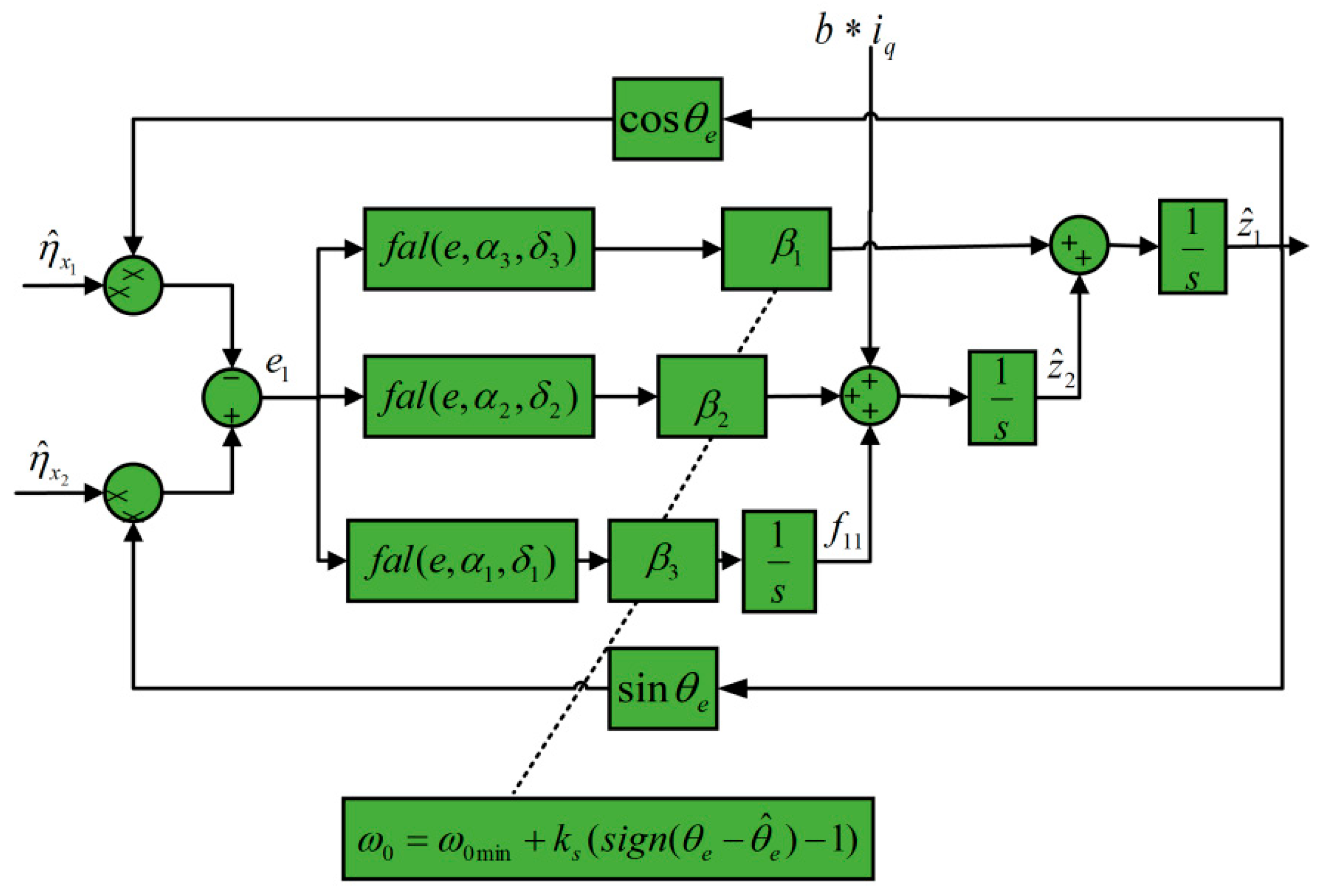
To address the above issues, this study introduces a speed estimation method based on a third-order ANLESO. It uses nonlinear functions to handle errors. According to Equation (32), the designed third-order ANLESO system can be expressed as follows:

$$\left\{\begin{array}{l}{e}_1=\theta -\widehat{\theta }\\ \dot{\widehat{\theta }}={\widehat{\omega }}_e+{\beta }_{1}fal(e_1,0.5,\delta )\\ {\dot{\widehat{\omega }}}_e=\widehat{z}+b{i}_q^{*}+{\beta }_{2}fal(e_1,0.5,\delta )\\ \dot{\widehat{z}}={\beta }_{3}fal(e_1,0.25,\delta )\end{array}\right.$$

(38)

The nonlinear function $fal(e_1,a,\delta )$ is defined as follows:

$$fal(e_1,a,\delta )=\left\{\begin{array}{l}\begin{array}{ll}{\displaystyle \frac{e_1}{{\delta }^{1-\alpha }}},& \left|e_1\right|\le \delta \end{array}\\ \begin{array}{ll}{\left|e_1\right|}^{\alpha }\mathrm{sgn}(e_1),& \left|e_1\right|>\delta \end{array}\end{array}\right.$$

(39)

Next, the error expression of the third-order ANLESO is further derived as follows:

$$\left\{\begin{array}{l}{\dot{e}}_1=e_2-{\beta }_{1}fal(e_1,0.5,\delta )\\ {\dot{e}}_2=e_3-{\beta }_{2}fal(e_1,0.5,\delta )\\ {\dot{e}}_3=h-{\beta }_{3}fal(e_1,0.25,\delta )\end{array}\right.$$

(40)

To ensure the stability of system dynamics and enhance its ability to counteract noise disturbances, the steady-state error should be within the nonlinear interval $\delta <e_1$ of the nonlinear function $fal(e_1,0.25,\delta )$. When the system reaches a stable state, the right-hand side of Equation (40) will tend towards zero. Based on this condition, Equation (20) can be restated as follows:

$$\left\{\begin{array}{l}{e}_2-{\beta }_1{\left|e_1\right|}^{0.5}\mathrm{sgn}(e_1)=0\\ e_3-{\beta }_2{\left|e_1\right|}^{0.5}\mathrm{sgn}(e_1)=0\\ h-{\beta }_3{\left|e_1\right|}^{0.25}\mathrm{sgn}(e_1)=0\end{array}\right.$$

(41)

Thus, the steady-state error of the third-order ANLESO can be expressed as

$$\left\{\begin{array}{l}{e}_1={\left({\displaystyle \frac{h}{{\beta }_3}}\right)}^4\mathrm{sgn}\left(h\right)\\ e_2={\beta }_1{\left({\displaystyle \frac{h}{{\beta }_3}}\right)}^2\mathrm{sgn}\left(h\right)\\ e_3={\beta }_2{\left({\displaystyle \frac{h}{{\beta }_3}}\right)}^2\mathrm{sgn}\left(h\right)\end{array}\right.$$

(42)

From the analysis of Equation (42), under the same conditions β₃ > h, the ANLESO method shows a smaller steady-state error than the LESO method.

By deriving the transfer function from Figure 6, the phase error transfer function can be obtained as follows:

$$G_e^{ANLESO}(s)={\displaystyle \frac{\theta -\widehat{\theta }}{\theta }}={\displaystyle \frac{s^3}{s^3+{\beta }_{\tau 4}{s}^2+{\beta }_{\tau 5}s+{\beta }_{\tau 6}}}$$

(43)

where ${\beta }_{\tau i}={\beta }_{i}fal(e_1,a_i,\delta )$.

For input signals experiencing frequency ramp variations, the steady-state phase error of the third-order ANLESO is calculated as follows:

$$\Delta {\theta }_{ess}^{ANLESO}(s)=\underset{s\to 0}{\lim }({\displaystyle \frac{s^3}{s^3+{\beta }_{\tau 4}{s}^2+{\beta }_{\tau 5}s+{\beta }_{\tau 6}}}\cdot {\displaystyle \frac{n}{s^3}})\cdot s=0$$

(44)

For the conventional LESO, by performing a Laplace transform on the LESO error equation and simplifying, the ratio of the estimated disturbance to the actual disturbance can be obtained as follows:

$${\displaystyle \frac{f_{11}(s)}{f(s)}}={\displaystyle \frac{{\beta }_3}{s^3+{\beta }_1{s}^2+{\beta }_{2}s+{\beta }_3}}$$

(45)

From Equation (45), the disturbance error transfer function of the LESO is obtained as follows:

$${\displaystyle \frac{f(s)-f_{11}(s)}{f(s)}}={\displaystyle \frac{s^3+{\beta }_1{s}^2+{\beta }_{2}s}{s^3+{\beta }_1{s}^2+{\beta }_{2}s+{\beta }_3}}$$

(46)

In this paper, when replacing the conventional magnetic flux PLL with a third-order ANLESO, performing a Laplace transform on the ANLESO error equation and simplifying yields the ratio of estimated to actual disturbance:

$${\displaystyle \frac{f_{11}(s)}{f(s)}}={\displaystyle \frac{{\beta }_{\tau 6}}{s^3+{\beta }_{\tau 4}{s}^2+{\beta }_{\tau 5}s+{\beta }_{\tau 6}}}$$

(47)

From Equation (47), the disturbance error transfer function of the third-order ANLESO can be obtained as follows:

$${\displaystyle \frac{f(s)-f_{11}(s)}{f(s)}}={\displaystyle \frac{s^3+{\beta }_{\tau 4}{s}^2+{\beta }_{\tau 5}s}{s^3+{\beta }_{\tau 4}{s}^2+{\beta }_{\tau 5}s+{\beta }_{\tau 6}}}$$

(48)

As per Equation (46), the Bode plot of the third-order LESO disturbance error is presented as follows:

As shown in Figure 7, as parameter w₀ increases, the disturbance error of the traditional third-order LESO also increases. The disturbance error rate is low in the high-frequency band, so the estimated disturbance cannot effectively reflect the actual disturbance’s changes across the entire range. Also, this feature is observed in the mid-frequency band, and in the high-frequency band, the phase lag is about 90°.

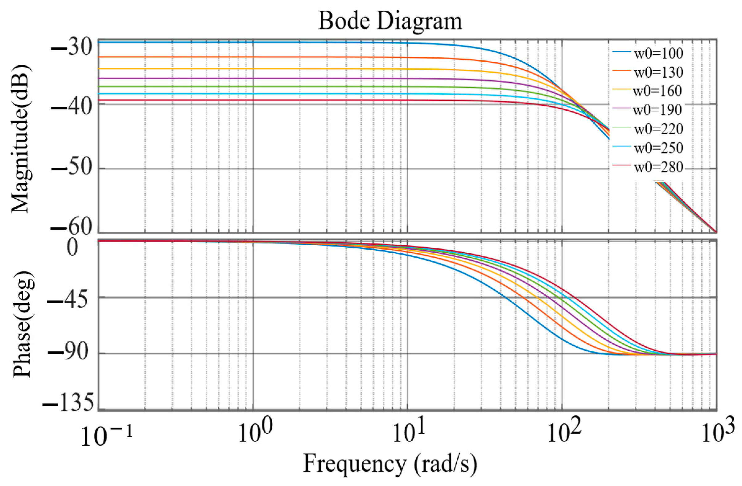
The Bode plot of the third-order ANLESO disturbance error, constructed based on Equation (48), is presented as follows:

In most cases, the disturbance frequency is the motor’s fundamental frequency. According to Figure 8, the disturbance error rate of ANLESO in the middle-frequency band is lower than that of traditional LESO; the disturbance error rate in the high-frequency band is higher, that is, the estimated disturbance energy reflects the actual disturbance. Furthermore, in the high-frequency region, its phase lag is close to zero.

The pole placement technology can be used for third-order ANLESO gain design as follows:

$$\left\{\begin{array}{l}{\beta }_1=3{\omega }_0\\ {\beta }_2=3{{\omega }_0}^2\\ {\beta }_3={{\omega }_0}^3\end{array}\right.$$

(49)

In Formula (49), the bandwidth parameters w₀ of third-order ANLESO are defined. After multiple parameter adjustments based on empirical formulas and combined with actual conditions, it was found that using this ANLESO method has many advantages: it can not only estimate $\theta$, w_e and the total interference f₁₁ situation based on the measured signal, but also compare with traditional ESO technology, while improving the observation accuracy of interference factors, it can also effectively suppress the measurement amplification effect caused by noise. Adaptive bandwidth technology is designed to achieve rapid convergence while ensuring sufficient noise to improve system control performance. For third-order ANLESO, the bandwidth parameters are established according to the following equation:

$${\omega }_0={\omega }_{0\min }+k_s(sign({\theta }_e-{\widehat{\theta }}_e)-1)$$

(50)

In this expression, the defined minimum bandwidth value ${\omega }_{0\min }$ is introduced and a parameter $k_s$ is introduced to adjust the bandwidth. The relevant control system structure is shown in Figure 9:

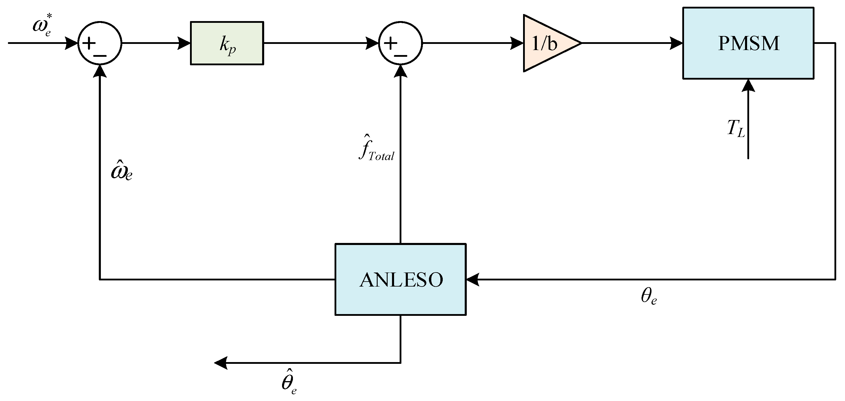
3.4. Error Feedback Control Law Design

The linear state error feedback control law (LSEFCL) is designed according to the following steps:

$$u_0=k_p\cdot ({{\omega }_e}^{\ast }-{\widehat{\omega }}_e)$$

(51)

where u₀ is the output signal of the system; ${{\omega }_e}^{\ast }$ and ${\widehat{\omega }}_e$ are the set value and estimated value of the speed; k_p is the gain parameter.

After corresponding compensation for perturbation factors in the entire system, it can be concluded that the specific expression of the control variable is

$$i_q=(u_0-\widehat{z})/b$$

(52)

where the total system interference $\widehat{z}$ covers all external and internal interference.

As shown in Figure 10, it can be observed from the figure that the speed control link only depends on a single parameter setting, thus simplifying the complexity problem in the adjustment process.

According to the aforementioned analysis, in order to achieve the purpose of accurate observation, the LESO scheme requires a higher gain setting, but this may also make the system noise-sensitive. To meet this challenge, this paper introduces a third-order ANLESO design, explains the working principle, and designs an LSEFCL-based ADRC controller to form adaptive nonlinear self-immune control (ANLADRC).

3.5. Stability Analysis of ANLESO

The error equation of third-order ANLESO can be deduced as [36,37]:

$$\dot{e}=Ae+Bh$$

(53)

where $e={\left[\begin{array}{ccc}{e}_1& e_2& e_3\end{array}\right]}^T$, $A=\left[\begin{array}{ccc}-{\beta }_1& 1& 0\\ -{\beta }_2& 0& 1\\ -{\beta }_3& 0& 0\end{array}\right]$, $B={\left[\begin{array}{ccc}0& 0& 1\end{array}\right]}^T$.

To make matrix A a Hurwitz matrix, the following conditions need to be met:

$${\beta }_1{\beta }_2-{\beta }_3>0$$

(54)

When the condition (54) is established, the observer exhibits asymptotic stability. According to the analysis of Formulas (2)–(24), it can be seen that meeting the condition (54) is relatively easy to achieve.

From Formulas (38), (40) and (53), you can obtain

$$\dot{\epsilon }=-c\epsilon +B_{2}e$$

(55)

In the formula, $\epsilon ={\omega }_e^{*}-{\omega }_e$, $B_2={\left[\begin{array}{ccc}0& -c& -1\end{array}\right]}^T$.

From this, we can obtain

$$\left[\begin{array}{l}\dot{\epsilon }\\ \dot{e}\end{array}\right]=\left[\begin{array}{cc}-c& B_2\\ 0& A\end{array}\right]\left[\begin{array}{l}\epsilon \\ e\end{array}\right]+B_{3}h$$

(56)

where $B_3={\left[\begin{array}{ccc}0& 0& \begin{array}{cc}0& 1\end{array}\end{array}\right]}^T$, definition $C=\left[\begin{array}{cc}-c& B_2\\ 0& A\end{array}\right]$.

Given that A is a Hurwitz matrix and c is a positive constant, it can be confirmed that C also has the characteristics of a Hurwitz matrix. In addition, the closed-loop control system described in Formula (56) shows the characteristics of asymptotic stability.

4. Simulation Analysis

4.1. Simulation Model Construction

In order to evaluate the effectiveness of the proposed third-order ANLESO, based on the design scheme of the observer (see Figure 11), based on the Simulink platform, this paper conducts a comparative simulation test of various control methods. For details of the motor parameters used in these simulation experiments, see

Table 1. LESO and ANLESO simulation parameters.

Parameter	LESO	ANLESO
Speed ring gain kp	220	985
ESO Compensation coefficient b	30,000	29,800
ESO Gain w0	180	——
Adaptive Gain ks	——	35
Bandwidth w0min	——	45

.

To evaluate the effect of the PI control strategy, the proportional gain of the motor speed ring is set to 0.005, and the integral gain is adjusted to 0.03; the proportional gain of the current control loop is set to 0.5, and the integral gain is 235. For the PLL part, its proportional gain value is determined to be 220 and the integral gain is 3950. In addition, the magnetic flux observer uses 6000 as the gain coefficient. For specific simulation parameters of LESO and ANLESO, see Table 1. The parameters of the PI controller can be designed as

$$k_p=L/2T,k_i=R/2T$$

(57)

$$k_{cp}=3J/(5T_{d2}{k}_t),k_{ci}=3J/(25T_{d2}^2{k}_t)$$

(58)

$$k_{sp}=2\zeta {\omega }_n,k_{si}={\omega }_n^2$$

(59)

where Equation (57) is used for the design of PI controller in PLL, where L represents inductance, H; R is the resistance, Ω; T is the sampling period, s. Equation (58) is the design of the PI parameters of the current loop, where J is the moment of inertia, kg·m²; T_d2 = T_d + 2T, k_t is the motor torque constant, which refers to the proportional relationship between the electric signal input by the motor and the output torque. Equation (59) is the design of the PI parameter of the velocity loop, where J is the moment of inertia, kg·m²; ζ is the damping ratio and w_n is the natural frequency.

4.2. Results Analysis

The performance of PLL-based PI control, LADRC, and ANLADRC under the condition that the motor speed increased from 900 rpm to 1500 rpm was thoroughly analyzed. The relevant results are shown in Figure 12, Figure 13 and Figure 14. These charts compare actual and estimated motor speed, speed error, angle, and error, respectively.

By observing Figure 12a, Figure 13a and Figure 14a, it can be found that PLL exhibits about 9% overshoot when the rotational speed changes abruptly, and can return to a stable state within about 0.2 s. In contrast, neither LADRC nor the optimized ANLADRC showed significant overshoot, in which the traditional method can reach a steady state within 0.1 s, while the optimized method can complete the adjustment in only 0.03 s, which is mainly due to the use of ANLESO technology to increase the order of the phase-locked loop, thereby enhancing the dynamic response of the system.

As can be seen from Figure 12b, Figure 13b and Figure 14b, the steady-state error generated by the traditional PLL can reach about 20 rpm after experiencing a speed jump, while the corresponding value of the LADRC is controlled to fluctuate within 10 rpm, and the further optimized scheme reduces this value to 4 rpm, which significantly improves the measurement accuracy. In addition, as shown in Figure 12c,d and Figure 14c,d, there is a certain lag between the actual and predicted angles under the traditional PLL method, and the difference range is about 0.15 rad. For LADRC, this gap narrows to within 0.1 rad; with the improved algorithm, the maximum deviation between the two is further reduced to 0.02 rad. In summary, the ANLADRC method based on ANLESO proposed in this study can effectively improve the accuracy of the estimation of rotor position and velocity information.

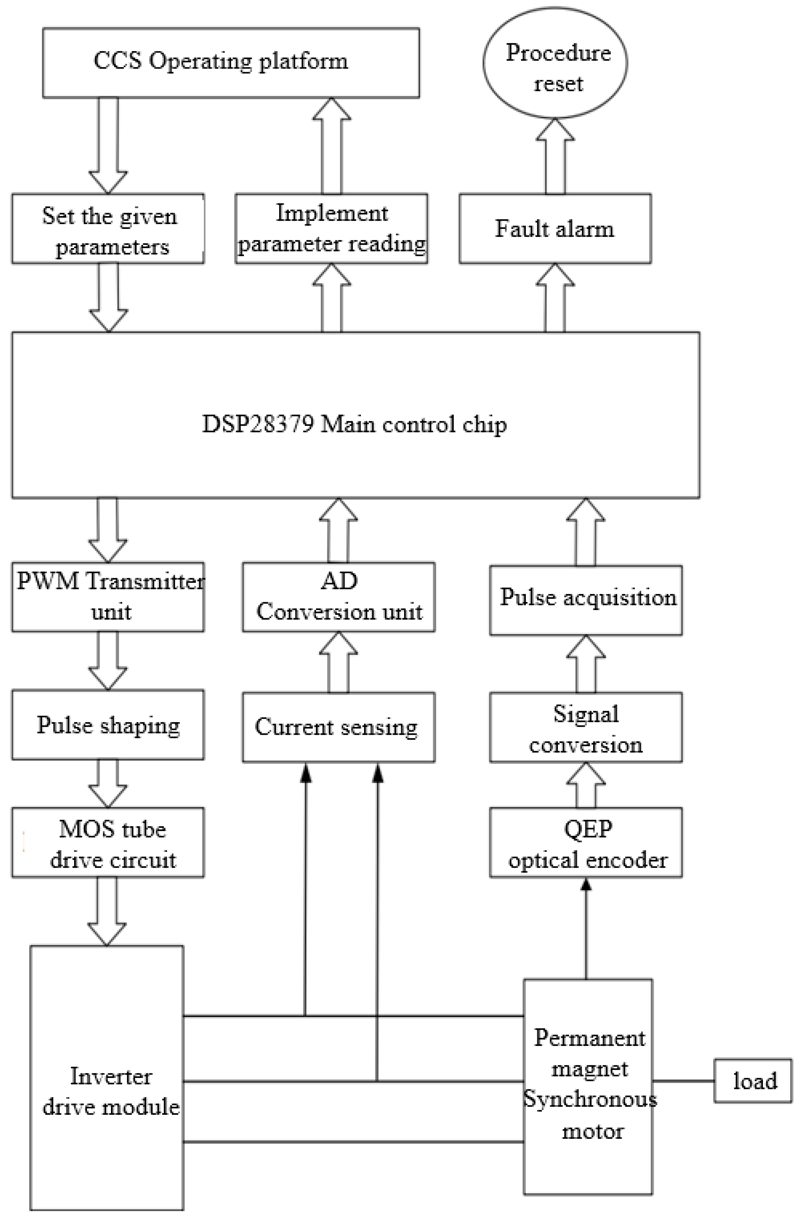
5. Design and Experiment of Permanent Magnet Synchronous Motor Control System

In order to analyze the performance of the two algorithms proposed in this paper in practical applications, a TMS320F28379D model microcontroller is selected in this chapter, and a number of hardware modules are designed based on this. good. Furthermore, by using the integrated development environment provided by Texas Instruments - Code Composer Studio (hereinafter referred to as CCS), the software design of the entire system was completed. 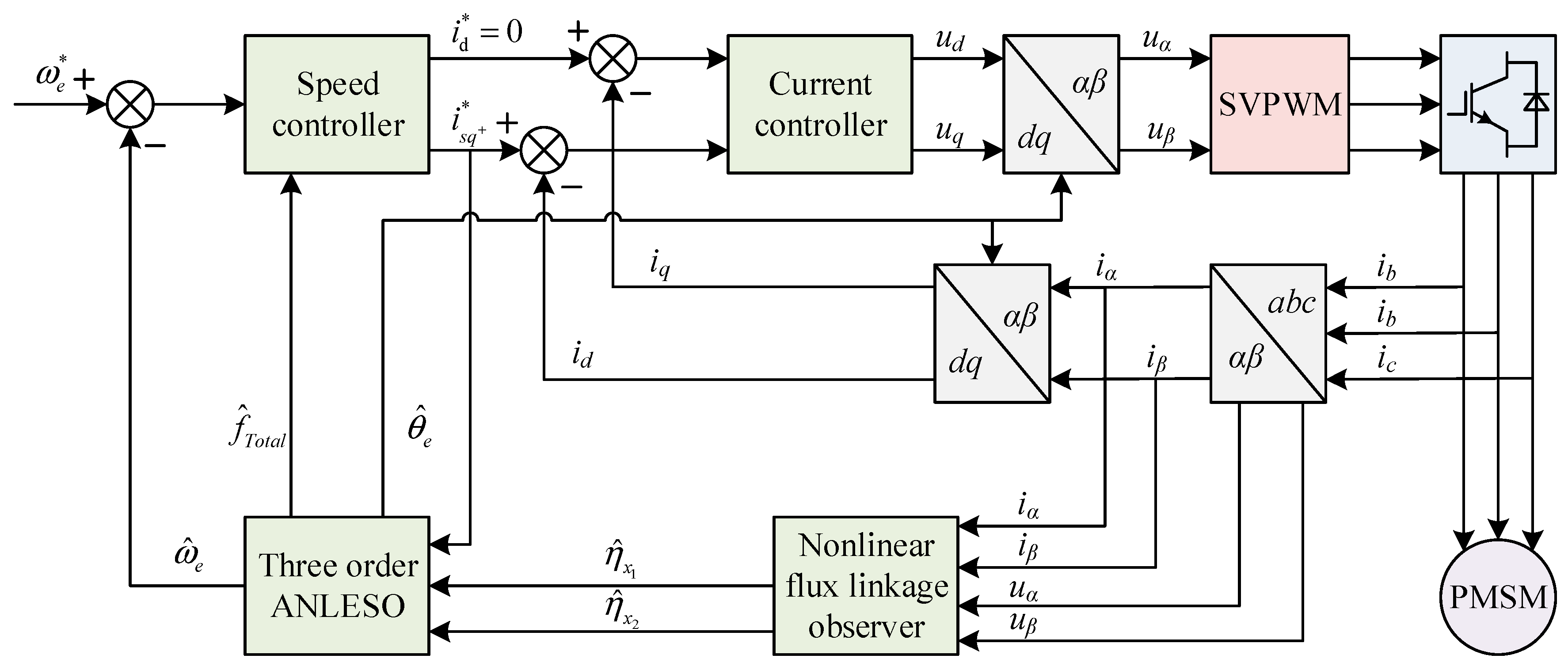Figure 15 shows the structural block diagram of the control system.

5.1. Software Design Process

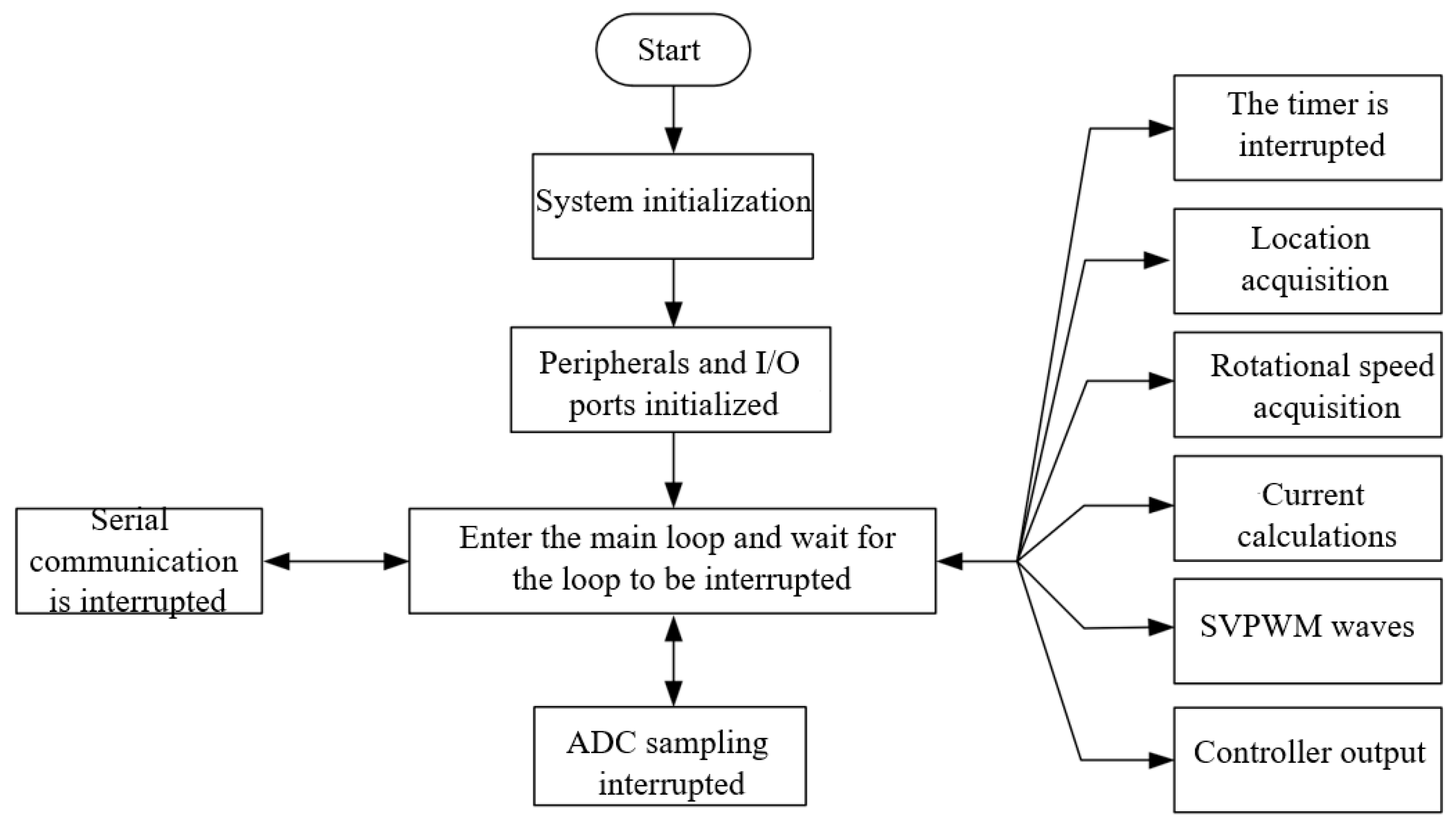
5.1.1. Main Programming Process

In this paper, CCS software 12.2.0 is used as a programming tool for the development of a permanent magnet synchronous motor control program. The programming process covers system initialization, peripheral and IO port configuration, and main-loop mechanism. In the main loop, the system waits until the interrupt signal is triggered. Subsequently, a series of tasks are performed in the interrupt service routine, including data acquisition of motor position and speed, calculation of current values, and generation of SVPWM waveforms. The entire software architecture is shown in Figure 16.

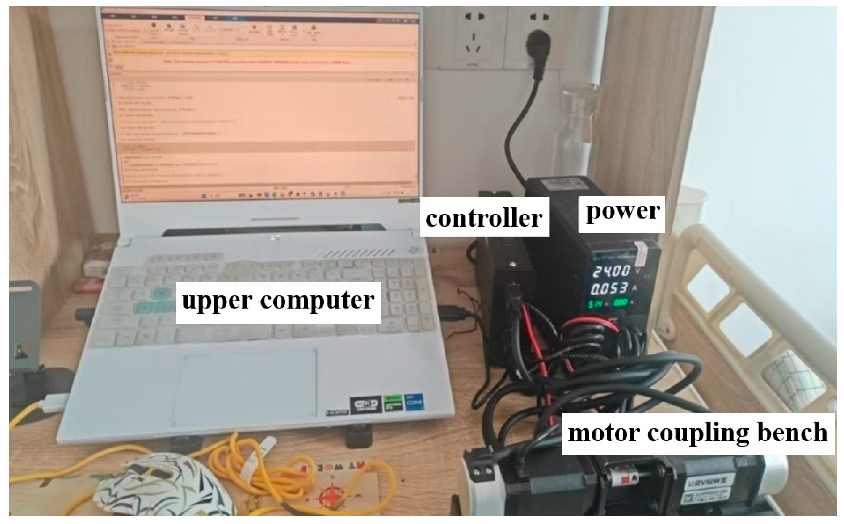
5.1.2. Experimental Platform

Figure 17 shows the experimental platform for verifying the control strategy.

5.2. Analysis of Experimental Results

In terms of experimental Settings, both the PWM carrier frequency and the current sampling frequency were set to 10 k Hz, and a dead time of 1.2 μs was also set. The main control board has two DAC output channels. For high-frequency signals, DAC output is adopted and data acquisition and display are carried out through an oscilloscope. When a large amount of data needs to be processed, information is sent to the upper computer at a baud rate of 921,600 through the UART serial port, and the data group is transmitted once every 500 μs.

This experiment focused on the process of rotational speed variation. Set the switching frequency f_PWM of the driver to 10 k Hz, and configure the specific values of several algorithms based on the actual parameters. It is assumed that there is no influence on parameter deviation.

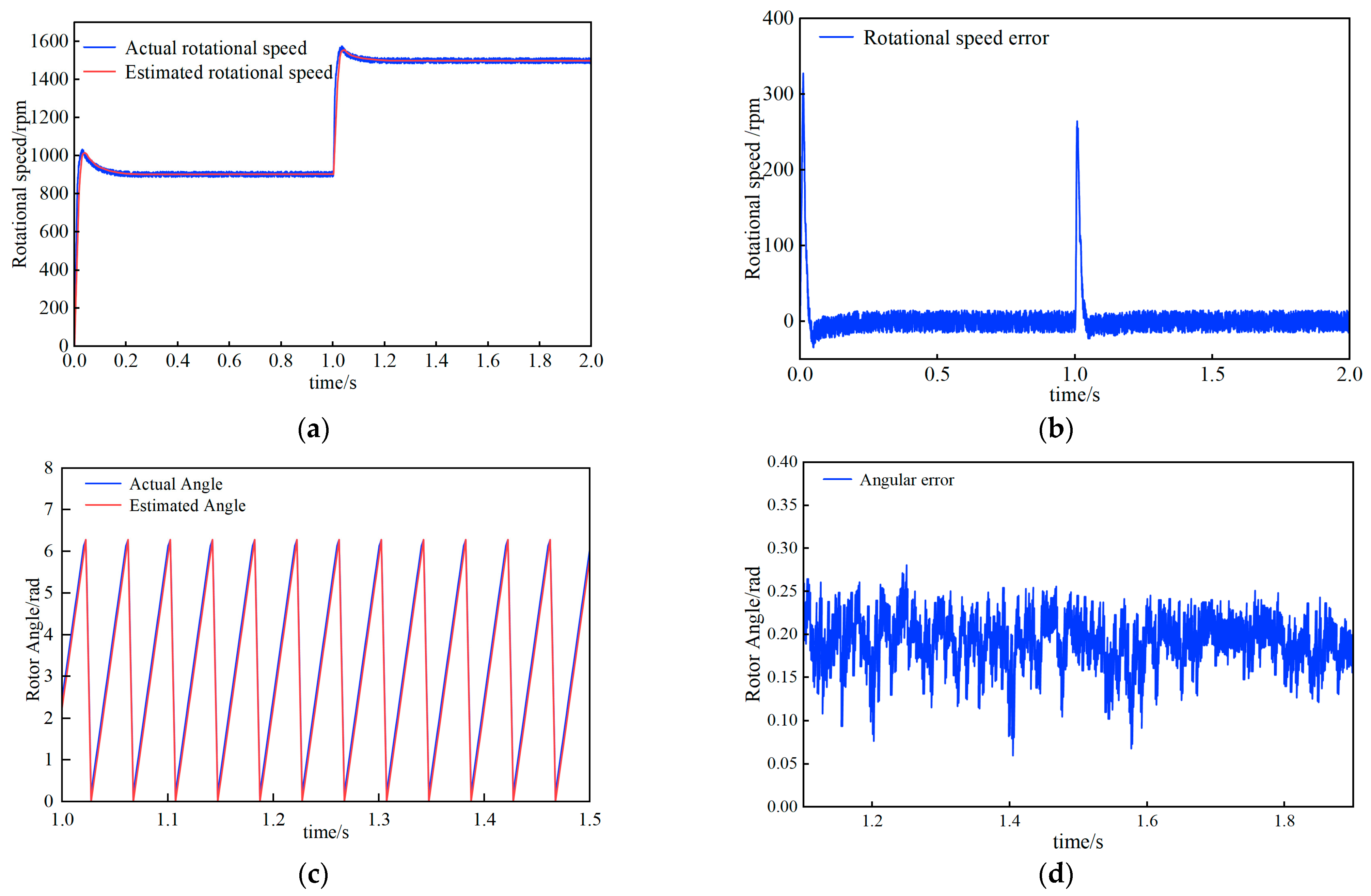
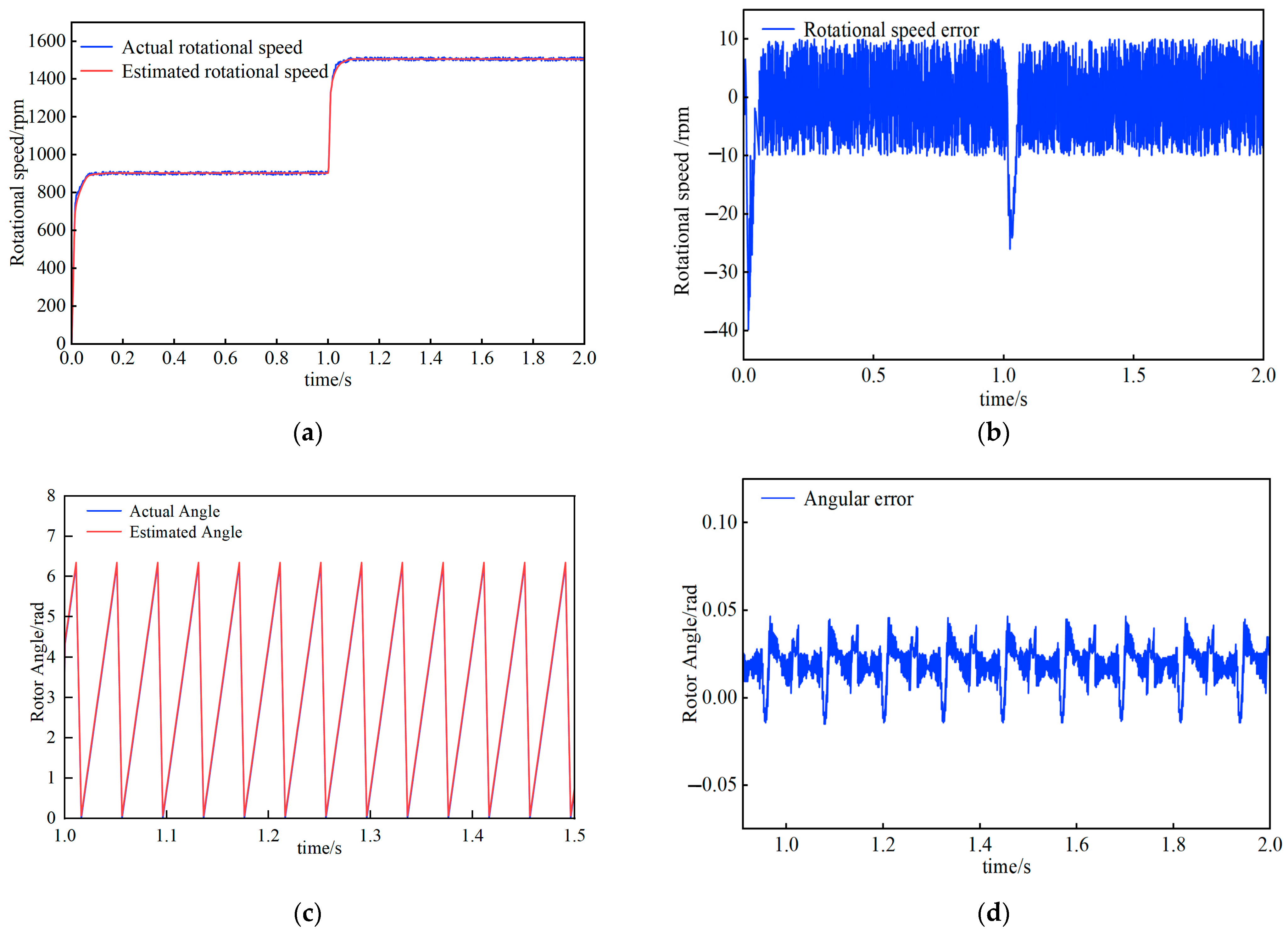
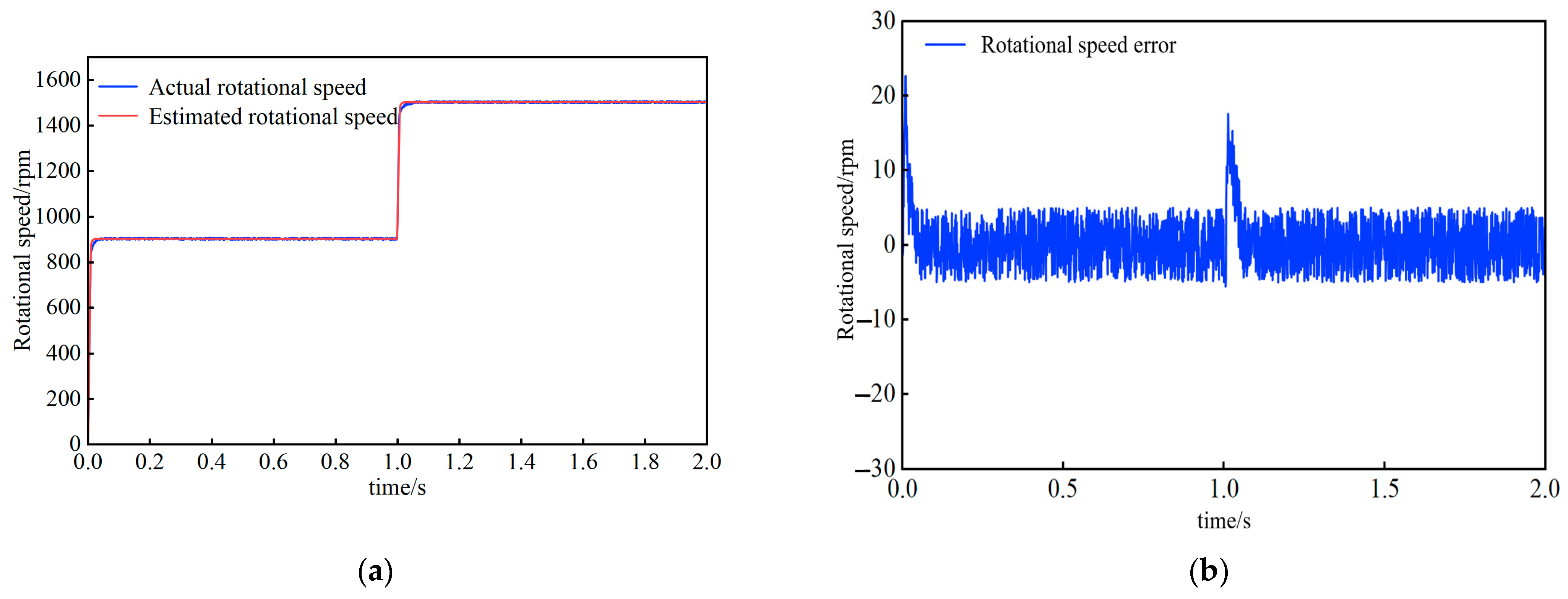
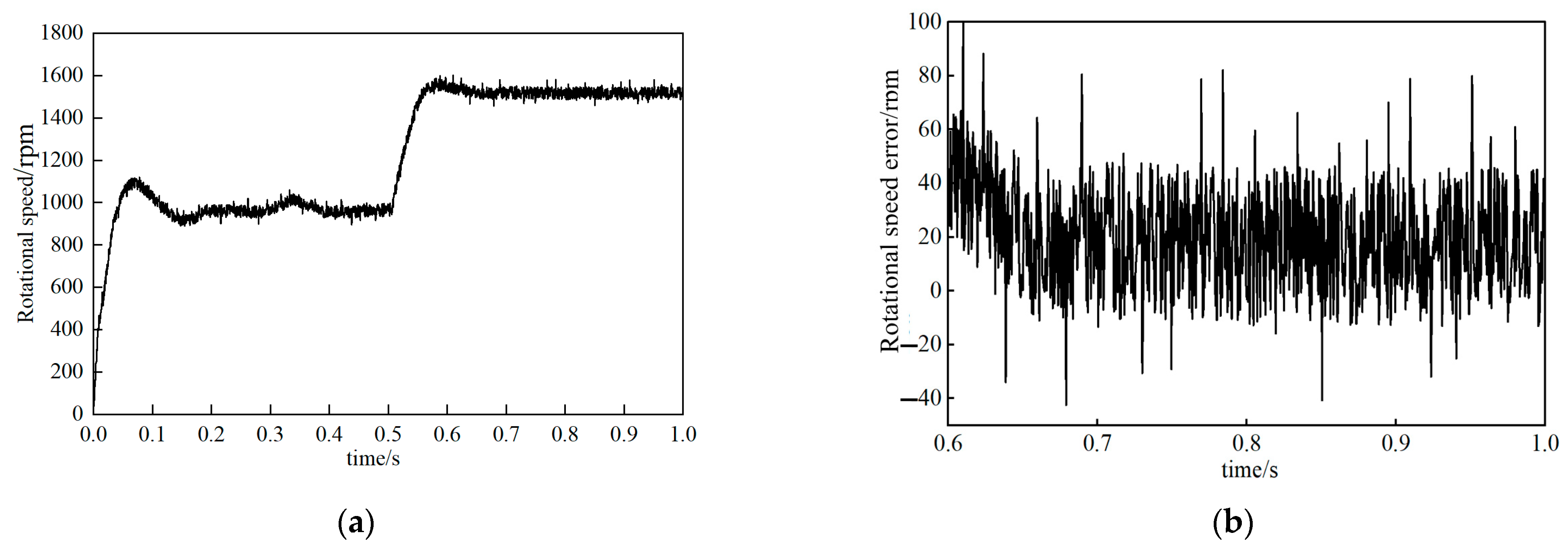
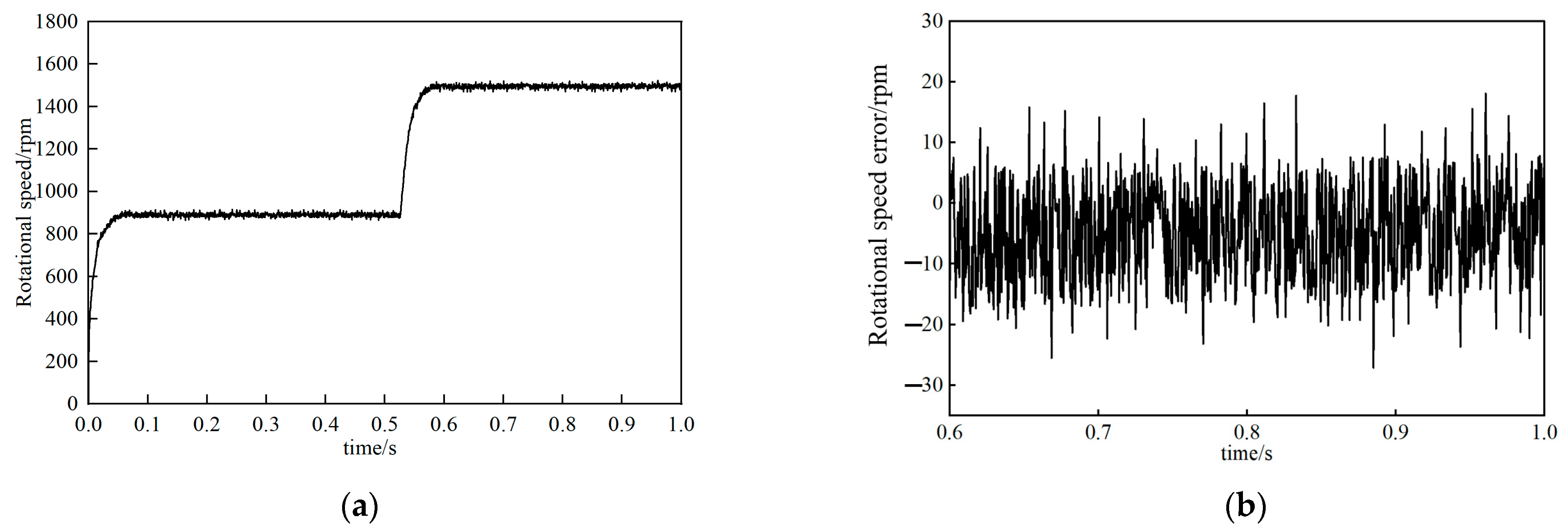
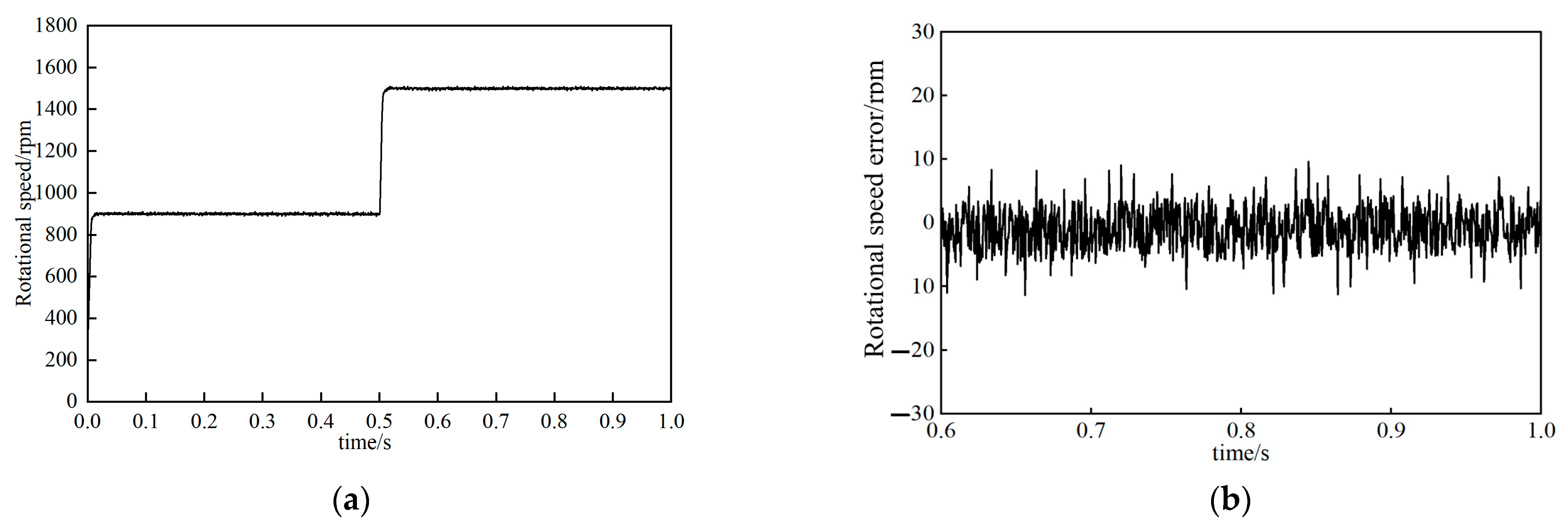
In the experiment, the motor jumped from order 0 to 900 rpm and ran for 0.05 s, then jumped again to 1500 rpm. Relevant data were recorded during this period. Through a detailed analysis of the rotational speed error of the motor in the final stable state, the aim is to verify the performance of the two proposed observers in various indicators. Specifically, during the speed step process, key indicators such as the PMSM acceleration characteristics, overshoot degree, and response time of the motor were investigated; After reaching the steady state, the focus is on studying the fluctuation of rotational speed and the difference between it and the preset target value. In order to ensure a fair comparison of the effects of the two proposed methods, the current regulator and speed controller PI settings unified with those of the control method were adopted throughout the entire testing process.

By observing Figure 18a, Figure 19a and Figure 20a it can be found that the traditional PI shows approximately 11% overshoot when the rotational speed suddenly changes from 0, and can fluctuate greatly at 900 rpm after the speed step. In contrast, neither LADRC nor ANLADRC showed obvious overshoot phenomena, and the errors were smaller. LADRC reached the steady state within 0.05 s, while ANLADRC adjusted to 900 rpm in just 0.03 s. It can be seen from Figure 18b, Figure 19b and Figure 20b that when the step jumps from 900 rpm to 1500 rpm, the PI rotational speed error is concentrated at 50 rpm, the LADRC is concentrated at 5 rpm–15 rpm, and the ANLADRC is concentrated at 3 rpm–5 rpm. ANLADRC has demonstrated outstanding performance in terms of adjusting time, overshoot, and the rotational speed error index after stable operation at 1500 rpm.

6. Conclusions

To enhance the dynamic response capability and robustness of sensorless submersible permanent magnet synchronous motors, this paper proposes an ANLADRC method based on ANLESO. The classic phase-locked loop technology is replaced by ANLESO to accurately estimate the speed, position, and overall interference amount. The stability of the proposed ANLESO scheme was verified through the analysis of the Hurwitz stability criterion. The simulation results show that it can effectively enhance the dynamic characteristics of the system. It verifies that the proposed strategy, under the condition of continuous steps of rotational speed, shows excellent performance in transient response, overshoot, and rotational speed error after stable operation compared with the traditional PI and LADRC. A motor control experimental system based on the TMS320F28379D digital signal processor was built. For the proposed algorithm, a continuous speed step experiment was carried out. The motor started from zero, first started to 900 rpm, and then stepped again to 1500 rpm. The proposed ANLADRC based on ANLESO has a rotational speed error of approximately 5 rpm and a response time of 0.03 s. Experiments have verified the effectiveness of the proposed sensorless control strategy and algorithm under complex working conditions.