Abstract
This research addresses the challenge of precise trajectory tracking for cart–pendulum robotic systems affected by unknown nonlinear actuator dynamics. We introduce a novel control framework that combines neural network modeling with adaptive parameter estimation to handle these complex dynamics. By characterizing state-dependent actuator behavior through custom-designed linear filters and adaptive laws, our approach identifies system parameters with high precision. We then develop an innovative fixed-time adaptive sliding mode controller that guarantees convergence within a predetermined timeframe regardless of initial conditions. Lyapunov stability analysis confirms that tracking errors converge to a small neighborhood around zero within the specified time bounds, with the size of the neighborhood determined by the design parameters. Simulation studies on a watermelon transportation robot validate our approach’s practical effectiveness, demonstrating improved tracking accuracy and robustness against actuator disturbances compared with conventional methods.
1. Introduction
In recent years, researchers have increasingly focused on addressing the challenges associated with trajectory tracking control for cart–pendulum robotic systems. Most of these robots are deployed in industrial and agricultural fields, where they are subjected to disturbances, noise, and actuator faults. In such environments, forcing the robot to follow a desired trajectory to meet the control objectives is extremely challenging. Moreover, the mathematical model of the cart–pendulum robot is often oversimplified as a linear quadratic system. Consequently, inaccuracies in the robot parameters lead to instability during control processes [1,2,3,4]. Additionally, once the actuator dynamics in robotic systems are perturbed, the entire system may collapse, posing a major threat to economic production, making advanced control indispensable. In particular, the adaptive techniques developed in [5,6,7] for system reliability and the advancements in sliding mode control techniques for robots [8,9,10,11] guide us in addressing trajectory tracking issues for the cart–pendulum robot. Similarly, in the domain of other motion control systems, researchers have tackled analogous challenges involving uncertainties and complex dynamics. For instance, the paper [12] developed a hybrid proximity control strategy for noncooperative spacecraft, employing an extended state observer and event-triggered sliding mode control to manage uncertainties in target behavior. Additionally, the work in [13] proposed a method for relative orbit transfer using constant-vector thrust acceleration, which addresses control under constraints. These works underscore the significance of robust control strategies in handling uncertainties, a principle that is equally applicable to our study of cart–pendulum robotic systems with bias actuator dynamics.
It is worth noting that recent studies have shown that integrating intelligent control technology with neural networks yields favorable results in countering nonlinear disturbances, including actuator dynamics and parameter uncertainties. In [14], an adaptively integral sliding mode control proposal based on fully connected recursive neural networks was introduced to stabilize the motion of a quadrotor aircraft. For nonsequential systems with time-varying state constraints, an intelligent adaptive control law using neural network techniques to approximate nonlinear functions was proposed in [15] to achieve path-following control. Furthermore, the method presented in [16] employed an iteratively flexible dynamic planning control strategy coupled with a segmented observer based on neural networks to address denial-of-service attacks and to identify complex time series. On another front, sliding mode control and self-adaptive technologies with strong anti-interference capabilities have proven effective in maintaining robotic stability. In order to resolve the challenge of distributed security control under network attacks, an adaptive elastic control algorithm was proposed in [17]. In [18], an anti-jamming sliding mode control scheme was developed to realize the path-following of the cart–pendulum robot.
In addition, while existing studies (e.g., [19,20]) have achieved finite-time stability, it is of practical significance to ensure that robotic systems are stabilized within a fixed time so that the settling time does not depend on the initial state. For instance, a fixed-time path-following control scheme that combines adaptive parameter estimation with sliding mode surface technology was presented in [21], optimizing the linear quadratic tracking performance for the cart–pendulum robot within a fixed time. The paper in [22] designed a fixed-time observer to guarantee a maximum upper bound on the controller’s settling period, with its performance later verified in an experimental case of an unstable inverted pendulum system. Similarly, the work in [23] introduced a fixed-time control scheme based on a nonsingular terminal sliding mode surface for second-order systems, while the paper in [24] presented a model transformation method combined with a neural network-based fixed-time trajectory tracking regulator using minimum learning parameters.
While current research has made significant advances in trajectory tracking control and fixed-time stability, there remains a critical gap in addressing unknown nonlinear actuator dynamics within a fixed-time convergence framework. Existing approaches, such as those proposed in [21,22,23,24], either handle actuator dynamics without guaranteeing fixed-time convergence or achieve fixed-time stability without explicitly addressing complex actuator behavior. This gap is particularly problematic for cart–pendulum robotic systems operating in industrial and agricultural environments where both precise timing and robustness against actuator impairments are simultaneously required.
Based on these previous studies, it is evident that ensuring stable trajectory tracking under actuator dynamics within a fixed time is a valuable research problem. In developing our approach, we draw inspiration from methodologies presented in [25,26,27,28], incorporating neural networks and perturbation-rejection for implementing filtering techniques to overcome estimation challenges for unknown dynamic parameters as highlighted in [27]. Building upon control principles described in [29,30,31,32], we establish a control framework with predetermined convergence timeframes utilizing an integrated surface methodology, ensuring the robotic system accurately follows reference trajectories within specified time constraints. Through Lyapunov stability analysis, we demonstrate that tracking error signals in the cart–pendulum system converge to minimal neighborhoods around the origin within specified temporal boundaries. Our simulation validation using a watermelon handling mechanism further confirms the efficacy of our proposed control approach.
Having examined the relevant literature, we offer the following distinctive contributions:
- (1)
- Our approach differs from conventional neural network parameter estimation techniques discussed in [27] by implementing a filtering mechanism that captures estimation error data from system signals in real-time. We develop adaptive estimation protocols to precisely identify unknown dynamic parameters through this mechanism.
- (2)
- While traditional sliding mode methodologies described in [30] provide a foundation, our work extends these principles through an integrated approach incorporating parameter estimation. This strategy overcomes limitations in conventional sliding mode techniques’ reaching phases and effectively compensates for actuator dynamics effects while maintaining precise control performance.
- (3)
- Differing from the studies in [18] and acknowledging practical operational constraints, our control strategy incorporates time-bounded convergence principles, minimizing initial state dependency on settling duration and establishing predetermined convergence timeframes. This enhancement significantly strengthens robotic trajectory tracking resilience against bias actuator dynamics. Moreover, the conservative design that assumes the dynamic parameter shown in [25] is overcome by adaptive adjustment designs in this paper.
The subsequent sections of this paper are structured as follows: Section 2 introduces key mathematical foundations and establishes parametric models for both trajectory tracking and dynamics characterization in cart–pendulum robotic systems. Section 3 presents our control strategy based on adaptive neural network estimation techniques and integrated sliding methodologies. Section 4 demonstrates the practical implementation through simulated manipulator scenarios, validating our approach’s effectiveness. Section 5 provides concluding remarks on the research contributions.
2. Research Model with Preliminaries
This section presents the mathematical representation of the cart–pendulum robotic system and defines the control objectives for achieving precise trajectory following when subjected to unknown state-dependent actuator dynamics. We consider scenarios where the actuator input is affected by unknown dynamics , which is modeled using neural network approximation techniques.
2.1. Kinematic and Dynamic Formulation of Cart–Pendulum Robotic Architecture
The kinematic and dynamic behavior of the cart–pendulum mechanism can be formulated as a coupled rigid-body system with both translational and rotational degrees of freedom. Drawing upon established principles of mechanical systems analysis [33], the physical behavior of this robotic architecture is comprehensively described by the following differential equations:
The system variables appearing in these equations are defined in Table 1. For analytical convenience, this model can be transformed into the following linearized continuous representation:
where the state vector is defined as , with inertial matrix , input distribution matrix , damping matrix , stiffness matrix , and vector represents bounded external disturbances acting on the system.

Table 1.
System dynamics nomenclature and parameters.
2.2. Lemmas
Lemma 1.
For the following nonlinear continuous system:
with , and a continuous positive-definite and radially unbounded function satisfying the following condition
where α, β, , are positive constants, the nonlinear system can reach 0 in a fixed time, and the convergence time t satisfies
Lemma 2.
For the following nonlinear continuous system:
with , and a continuous positive-definite and radially unbounded function satisfying the following condition
where α, β, , , ξ are positive constants, it can be said that the nonlinear system is stable in a fixed time, and the convergence time t is bounded by
where ϑ is a positive definite constant satisfying . Moreover, the system state converges to a residual set, as shown below
This kinematic and dynamic representation establishes the foundation for our control system design, capturing the essential motion characteristics and force interactions within the cart–pendulum robotic architecture. The state-space formulation provides a mathematical framework that enables systematic analysis of the system’s behavior under various operating conditions and external influences.
2.3. Bias Actuator Dynamics
For our analysis, we consider actuator impairments characterized by continuous state-dependent bias. The modeling approach utilizes neural network representation as follows:
In this formulation, represents the control signals ultimately received by the actuator mechanism, while denotes the spurious control signal component introduced through actuator impairment. Consistent with the approach in [27], we parameterize this impairment signal using a neural network architecture:
where represents the predetermined activation function vector for the hidden neural layer, w constitutes the unknown neural network weight vector requiring estimation, and signifies the bounded approximation error inherent in the neural representation.
2.4. Control Intents
The primary objective of our approach is to develop a controller enabling cart–pendulum systems affected by actuator impairments to accurately trace desired trajectories within predetermined time boundaries. The reference trajectory that the system should follow is generated through the dynamic model:
where r represents the reference input signal. Based on this formulation, we define the tracking error between the actual and desired system states as
By incorporating the system dynamics from (2) and reference trajectory from (12) into this error definition (13), we derive the following error dynamics:
where we define , , , . This allows us to express the tracking error dynamics in state-space representation:
with the system matrix , , the input matrix , and the term .
By defining , we can further simplify the error dynamics (without considering the actuator dynamics yet) to
Note that incorporates the reference signal r and the scaled external disturbance .
From the derivation above, it is clear that to achieve the desired control performance, the tracking error system must converge stably. Specifically, within the fixed time , the tracking error should be reduced into a small residual set in practice, characterized by bounds dependent on system parameters and approximation errors.
Remark 1.
In practical systems, disturbances typically appear as bounded noise signals. In the actuator dynamics model (10), both disturbances and nonlinear dynamics signals participate in the control channel (when substituting (10) into (2) or (16)). However, since the dynamics signal cannot be simply treated as a bounded signal, a neural network is employed to approximate its effect.
Remark 2.
The actuator is a critical component for altering the controlled variable and is prone to unknown dynamics. Once an actuator is compromised, it immediately disrupts the controlled quantity, leading to unpredictable results. Therefore, a novel adaptive sliding mode compensation control strategy is designed in this paper to both eliminate the adverse effects of actuator dynamics and ensure that the system tracks the reference trajectory within a fixed time.
Having established the mathematical foundations and problem formulation for the cart–pendulum robotic architecture, we now proceed to develop our adaptive parameter estimation and sliding surface control methodology that addresses both the actuator dynamics compensation and trajectory tracking objectives within a guaranteed convergence timeframe.
3. Adaptive Parameter Estimation and Sliding Surface Control Synthesis
In this section, a comprehensive control framework is developed that synthesizes adaptive parameter learning mechanisms with robust sliding surface dynamics to compensate for actuator dynamics effects in cart–pendulum robotic systems. The approach develops in two phases: first, constructing a methodology to accurately identify unknown dynamic parameters, and then formulating a control strategy that guarantees fixed-time convergence while compensating for these effects of the unknown dynamics.
3.1. Neural Network-Based Parameter Identification for Dynamics Characterization
Neural networks provide an effective framework for approximating complex nonlinear functions through their inherent structural properties. For the identified dynamic signal in Equation (11), we can formulate its estimated representation as
where denotes the estimated weight vector, with the corresponding estimation error defined as .
Incorporating the neural network representation of the dynamics signal (10) and (11) into the tracking error dynamics from Equation (16), we substitute for u:
where , and represents the lumped uncertainty combining the neural network approximation error and the term (which contains the reference signal and external disturbances). This combined term is assumed bounded, i.e., for some positive constant .
To facilitate estimation of the unknown weight vector w, we implement the following linear filtering structure:
where represents a positive filter time constant, and , , and are the filtered versions of their respective signals. Applying this filtering operation to Equation (18), we obtain
where satisfies . From (19), . Substituting this into (22):
Rearranging gives
This formulation allows us to extract information about the unknown weight vector. To facilitate this extraction, we introduce auxiliary matrices P and Q with dynamics:
where is a positive design constant. The explicit solutions for these matrices are
Substituting (23) into the integral for :
Thus, we can establish the following relationship:
where
represents the filtered error term. Since and are bounded, and if is bounded (which occurs if e is bounded), then is bounded, i.e., for some positive constant .
The parameter estimation error information can now be expressed as
Based on this error information , we design the following adaptive update law for :
where is a positive definite gain matrix, and are positive constants related to convergence properties, I is an identity matrix of appropriate dimension, E is designed to ensure (or simply if u is scalar), s is the sliding surface variable defined later, and denotes the signum function.
Remark 3.
The selection of matrix E is critical for ensuring the controllability of the sliding variable dynamics through the condition . This invertibility requirement establishes a necessary coupling between the sliding manifold and control input directions. Mathematically, E must be chosen such that its row space intersects nontrivially with the column space of B. For instance, in the cart–pendulum system studied in Section 4, the input matrix is . A suitable choice for E is . This yields . Since , this choice guarantees the necessary property for the sliding mode control design.
3.2. Time-Bounded Convergent Sliding Mode Control Strategy
Addressing the actuator dynamics challenge described by Equation (18), we develop a composite control structure for :
where represents the nominal feedback component with gain matrix H (designed later), and constitutes the compensating component designed to counteract actuator dynamics and ensure bounded-time convergence.
To eliminate reaching-phase dynamics associated with conventional sliding mode approaches, we implement an integral sliding surface:
Setting and assuming (or designing H such that is stable and starting on the surface), the integral term aims to maintain if the system follows .
Differentiating this surface yields
Substituting and :
To achieve our control objectives, we structure the compensating component as
where is designed to cancel the estimated dynamics, and provides robustness and fixed-time convergence:
with positive constants , , , and .
Theorem 1.
Consider the cart–pendulum robotic system with tracking error dynamics (16) under bias actuator dynamics (10) and (11). When implementing the control architecture (32)–(37) with parameter estimation mechanism (31) and sliding surface (33), both the tracking error e and parameter estimation error converge and stabilize within a predetermined time interval .
Proof.
We establish the Lyapunov function:
Through algebraic manipulation and substituting , we derive
Substituting the control component from (37) yields
Let and choose such that and . Applying the inequality , we derive
where , , , .
By Lemma 2 and defining , we establish that converges to the minimal set for , with convergence time bounded by . This confirms fixed-time bounded convergence of both the sliding variable s and parameter estimation error , and consequently, the tracking error e. □
Remark 4.
According to persistent excitation (PE) principles, if the regression matrix (related to ) is persistently exciting, it ensures that for some positive for t sufficiently large. Therefore, by selecting , we can ensure that , which is used in the stability proof of Theorem 1. This condition is crucial for parameter convergence analysis in adaptive control.
The above analysis confirms that the system state converges to and remains on (or near) the sliding manifold. To determine the feedback gain matrix H in , we examine the ideal sliding condition , which implies if or stability holds. The stability of the system on the sliding manifold is governed by the equivalent control method. When holds, it follows from (35) that . This implies the equivalent compensating control , assuming is invertible (or using pseudo-inverse). The total equivalent control is . Substituting into the original error dynamics (18) yields
For stability of the error dynamics on the sliding manifold, we require the matrix to be Hurwitz. This can be achieved by designing H such that there exists a symmetric positive definite matrix P satisfying the Lyapunov inequality:
To find such an H using Linear Matrix Inequalities (LMIs), we perform a change in variables. Let (thus ) and let . Premultiplying and post-multiplying the inequality (44) by Q yields which simplifies to . Expanding this, . Substituting (so ), we arrive at the LMI in variables Q and K:
This LMI can be solved efficiently for Q and K. Once a solution is found, the state feedback gain is recovered as .
This completes our synthesis of an adaptive parameter estimation and sliding surface control framework that achieves fixed-time bounded trajectory tracking for cart–pendulum robotic systems under bias actuator dynamics.
To avoid singularity when , the term in (37) can be modified to , where is a small constant. Besides, since is typically unknown in practical applications, we can modify our control approach by replacing the fixed gain with an adaptive estimate :
where , , estimates the unknown bound according to the update law:
with positive constant . The weight estimation law (31) is correspondingly simplified by removing the terms related to :
Corollary 1.
Proof.
We establish the augmented Lyapunov function:
where . Differentiating and substituting from (35), (46)–(48), considering the case , we have:
Since and involves terms proportional to which are nonnegative or can be bounded, in the case of , we have
which implies , confirming that the sliding variable reduces into boundary . The convergence of depends on the stability of the dynamics on the sliding manifold. □
Remark 5.
To mitigate chattering phenomena associated with the discontinuous signum function in (31), (37) and (46), we can implement a continuous approximation in practice. A common approach is to replace with a saturation function , a smooth function like for a small positive parameter ε, or the sigmoid approximation , where b is a positive parameter controlling approximation accuracy.
4. Watermelon Manipulator Case Study and Control Performance Evaluation
To validate the practical applicability and performance characteristics of our proposed control methodology, we conduct a comprehensive case study using a watermelon transportation robotic manipulator system. This application represents an industrial implementation of the cart–pendulum architecture with practical constraints and operational requirements. Following the configuration framework established in [33], the physical parameters of this experimental platform are defined as follows: pendulum mass , cart mass , gravity center offset , pendulum moment of inertia , pendulum damping coefficient , and cart damping coefficient .
4.1. Simulation Results
The system experiences external disturbances represented as . Based on this configuration, the trajectory tracking error dynamics in Equation (16) are characterized by the following system matrices:
For the simulation, we initialize the trajectory tracking error as . The bias actuator dynamics is modeled as , which we approximate using an RBF neural network. The unknown ideal weight vector corresponding to this structure is assumed to be for simulation purposes in formulation (11).
Our implementation uses filter parameters and . The adaptive estimation mechanism (31) employs gain matrix with convergence parameters and . For the integrated surface dynamics, we select which ensures . The feedback parameter vector H is obtained by solving the LMI (45) yielding . The controller (32) with from (37) utilizes gains , , , and . Based on Lemma 2 and the derived constants , the theoretical convergence time bound is calculated as s (actual value depends on exact derivation of ). We employ a reference trajectory defined by .
The neural network approximator employs radial basis functions (RBFs) as activation functions to characterize the state-dependent bias actuator dynamics. The network structure consists of 4 hidden neurons with Gaussian activation functions:
where centers are systematically distributed across the expected error state space, chosen as , , , and . The width parameters are selected uniformly to ensure sufficient overlap between adjacent RBFs for smooth function approximation across the anticipated state space. Initial weight values are set to zero, , allowing the adaptive learning process defined in Equation (31) to identify the appropriate weight values during operation. This configuration provides sufficient approximation capability to model the bias actuator dynamics within the operational domain. The performance can be sensitive to the choice of fixed centers and widths . While chosen heuristically based on the expected error range in this study, adaptive tuning mechanisms for these parameters could potentially improve performance and robustness, representing an avenue for future work. In the simulation, to avoid chattering, the signum function in this paper was approximated using the continuous sigmoid approximation function with .
The evaluation methodology focuses on three key performance indicators: trajectory tracking accuracy, convergence time characteristics, and robustness against actuator impairments. The following analysis examines both transient and steady-state behavior of the controlled system under the proposed adaptive parameter estimation and bounded-time control framework. The simulation results illustrated in Figure 1 and Figure 2 demonstrate the system’s tracking error and motion trajectory dynamics, respectively. These results confirm that our proposed methodology successfully confines tracking errors within a bounded region during a predetermined timeframe, even under bias actuator dynamics. Figure 3 illustrates the dynamic behavior of the integrated sliding surface, which initializes near zero and ultimately stabilizes within a minimal error margin around zero, validating our theoretical analysis.
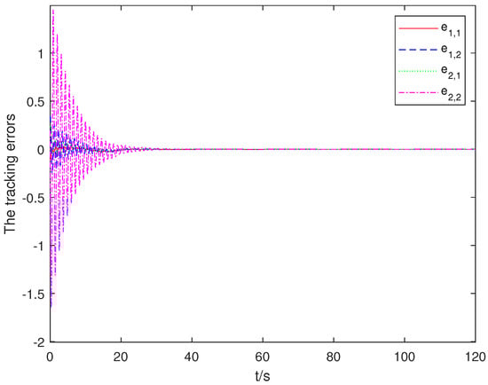
Figure 1.
Cart−pendulum robotic system tracking error dynamics under adaptive control. The errors and are in meters and radians for position and angle, respectively, and their derivatives are in m/s and rad/s.
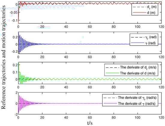
Figure 2.
Actual system trajectory versus reference path performance comparison. Positions are in meters and angles in radians versus time in seconds.
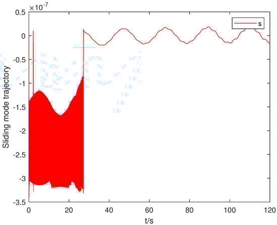
Figure 3.
Temporal evolution of the integral sliding manifold versus time in seconds (dimensionless).
Figure 4 depicts the temporal evolution of neural network weight parameter estimates, confirming bounded convergence within the specified timeframe. This demonstrates successful identification of the unknown dynamic characteristics, enabling the system to effectively counteract actuator impairments. Figure 5 shows the control input response, exhibiting appropriate stability characteristics throughout operation.
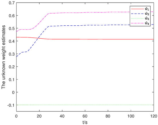
Figure 4.
Convergence behavior of neural network parameter estimates versus time in seconds (dimensionless).
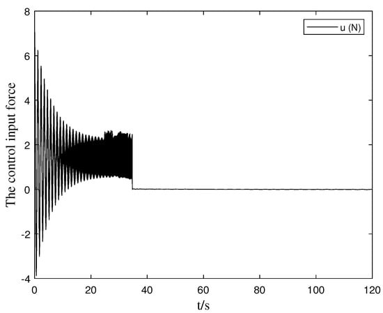
Figure 5.
Control input response during watermelon manipulator operation in Newton versus time in seconds.
These simulation results collectively validate that our proposed methodology enables effective time-bounded trajectory tracking control for cart–pendulum robotic systems operating under bias actuator dynamics. To further validate the efficiency and robustness of the proposed control technique, additional testing was performed by modifying the disturbances and bias actuator dynamics as and , respectively, where is a random value generated between [−1, 1]. The trajectory tracking error result is illustrated in Figure 6, which demonstrates the robustness of our approach under challenging conditions with significant random disturbances and time-varying actuator dynamics. Comparing Figure 1 and Figure 6, the controller maintains effective tracking performance, with the trajectory error converging rapidly to a small residual set within the theoretical bounds, despite the increased complexity of disturbances. Note that under these modified conditions, other responses (trajectory, sliding surface, weights, control input) exhibit similar bounded behavior as in Figure 2, Figure 3, Figure 4 and Figure 5 and are omitted for brevity. The robustness was partially tested by introducing these random and time-varying components. A more extensive Monte Carlo simulation varying system parameters (, etc.) could further quantify robustness, which is suggested for future investigation.
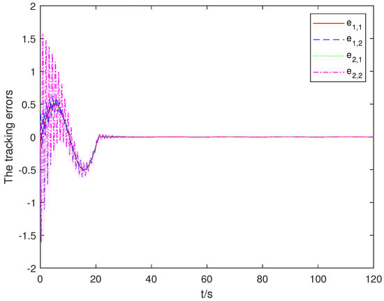
Figure 6.
Cart−pendulum robotic system tracking error dynamics under adaptive control by different disturbances and bias actuator dynamics. The errors and are in meters and radians for position and angle, respectively, and their derivatives are in m/s and rad/s versus time in seconds.
4.2. Comparative Analysis
To better demonstrate the advantages of the proposed method, we provide a quantitative comparison with selected existing approaches in [22,23,24] in Table 2. This table includes key performance metrics such as theoretical and actual convergence times, the convergence ratio (defined as the theoretical bound divided by the observed time, indicating conservativeness), Root Mean Square Error (RMSE) of the tracking error, and maximum overshoot.
Table 2.
Comparison of key performance metrics across methods. The convergence ratio is defined as the ratio of theoretical convergence time to actual convergence time. RMSE and Max Overshoot estimated for pendulum angle error . N/A indicates metrics not directly available or comparable from references, especially for actuator fault scenarios.
As shown in the comparison, while the method in [22] achieves fast actual convergence for its specific problem, its theoretical bound is highly conservative (large convergence ratio). Our method provides a less conservative theoretical convergence time estimate, with a reasonable gap between theoretical and actual convergence. Our method achieves good tracking accuracy (RMSE∼) with moderate overshoot, while explicitly handling the bias actuator dynamics, a challenge not directly addressed in the compared fixed-time control works [23,24]. Direct quantitative comparison of RMSE/overshoot with [22,23,24] is difficult due to differing system models, control objectives, and lack of reported metrics for actuator fault scenarios in those papers. However, the results demonstrate our method’s capability for accurate fixed-time tracking in the presence of actuator impairments.
The performance of our proposed methodology can be attributed to several key factors:
- The filtering-based parameter estimation approach enables accurate identification of the unknown actuator dynamics compared with methods relying solely on disturbance observers, effectively addressing the challenge of nonlinear actuator behavior.
- The integrated sliding surface design eliminates the reaching phase present in conventional sliding mode controllers, reducing transient tracking errors and providing consistent convergence behavior.
- The fixed-time control law guarantees convergence within a predictable time bound, independent of initial conditions, which is critical for time-sensitive applications.
Despite these advantages, our approach has certain considerations:
- The computational complexity is higher than conventional nonadaptive sliding mode methods due to the real-time neural network operations and filter dynamics, potentially limiting applicability in extremely resource-constrained systems.
- The control performance depends on appropriate selection of neural network structure (number of neurons, centers, widths) and adaptive/controller gains, requiring careful tuning.
- While simulations demonstrated robust performance, extreme actuator failures significantly exceeding the approximation capabilities of the neural network could potentially compromise system stability.
Practical implementation considerations include the computational load associated with the neural network updates and the filter dynamics. The RBF network requires function evaluations and vector operations proportional to the number of neurons, and the adaptive law involves matrix/vector operations. This should be feasible on modern embedded controllers for typical robotic sampling rates (e.g., 1 kHz). The LMI for gain H is solved offline. Hardware constraints might involve sensor noise affecting error signals and actuator saturation, which are not explicitly modeled here but could be addressed using standard techniques like input saturation or noise filtering.
5. Conclusions
This investigation has examined trajectory following capabilities with predefined convergence timeframes for cart–pendulum robotic mechanisms operating under actuator impairment conditions. We have introduced a filtering methodology to determine weight coefficients associated with neural network-approximated actuator anomalies. Subsequently, we have formulated a fixed-time bounded regulation approach leveraging integrated surface dynamics that effectively compensates for actuator impairments. This control architecture enables all dynamic variables within the closed-loop guidance system to attain constrained stability within predetermined temporal boundaries while simultaneously ensuring the controlled variables accurately follow reference paths. Verification through simulation modeling of a watermelon handling mechanism has substantiated the practical viability of our proposed regulatory approach.
These findings have significant implications for practical industrial and agricultural applications. The demonstrated capability extends to numerous material handling scenarios where precise motion control under unpredictable operating conditions is critical. Potential applications include:
- Automated harvesting systems operating in variable soil and crop conditions.
- Factory automation systems subject to maintenance-related actuator degradation.
- Collaborative robots working alongside humans, where predictable timing is essential for safety.
Future work will focus on hardware implementation on commercial robotic platforms and extension to multijoint manipulators, further bridging the gap between theoretical advances and practical deployment in challenging real-world environments. Additionally, exploring the integration of cascaded adaptive neuro-fuzzy inference system (ANFIS) techniques, such as those proposed in [34], with our fixed-time control framework could potentially enhance adaptation capabilities for systems facing complex, time-varying actuator dynamics over extended operational periods. Further robustness validation through extensive Monte Carlo simulations is also warranted.
Author Contributions
Conceptualization, X.J.; methodology, S.C. and X.J.; software, S.C.; validation, X.J. and H.W.; data curation, X.Z.; writing—original draft preparation, S.C.; writing—review and editing, X.Z. and H.W.; project administration, X.J.; funding acquisition, X.J. All authors have read and agreed to the published version of the manuscript.
Funding
This work is supported in part by the National Nature Science Foundation of China under grant 62173193; in part by the Taishan Scholars Program under Grant tsqn202211208; in part by the Science Education Industry Integration and Innovation Project under Grant 2024RCKY003; in part by the open research fund of Anhui Provincial Key Laboratory of Intelligent Low-Carbon Information Technology and Equipment.
Data Availability Statement
Data are contained within the article.
Conflicts of Interest
The authors declare no conflicts of interest.
References
- Faheem, M.; Liu, J.; Chang, G.; Ahmad, I.; Peng, Y. Hanging force analysis for realizing low vibration of grape clusters during speedy robotic post-harvest handling. Int. J. Agric. Biol. Eng. 2021, 14, 62–71. [Google Scholar] [CrossRef]
- Xu, S.; Yu, H.; Wang, H.; Chai, H.; Ma, M.; Chen, H.; Zheng, W.X. Simultaneous diagnosis of open-switch and current sensor faults of inverters in IM drives through reduced-order interval observer. IEEE Trans. Ind. Electron. 2024, 72, 6485–6496. [Google Scholar] [CrossRef]
- Jin, X.; Che, W.; Wu, Z.; Wang, H. Analog control circuit designs for a class of continuous-time adaptive fault-tolerant control systems. IEEE Trans. Cybern. 2020, 52, 4209–4220. [Google Scholar] [CrossRef]
- Jin, X.; Hou, Y.; Wu, X.; Chi, J. Adaptive ELM-based time-constrained control of uncertain robotic manipulators with minimum learning computation. IEEE Trans. Emerg. Top. Comput. 2025, 1–12. [Google Scholar] [CrossRef]
- Jin, X.; Lü, S.; Yu, J. Adaptive NN-based consensus for a class of nonlinear multiagent systems with actuator faults and faulty networks. IEEE Trans. Neural Netw. Learn. Syst. 2021, 33, 3474–3486. [Google Scholar] [CrossRef]
- Jin, X.; Wang, S.; Qin, J.; Zheng, W.X.; Kang, Y. Adaptive fault-tolerant consensus for a class of uncertain nonlinear second-order multi-agent systems with circuit implementation. IEEE Trans. Circuits Syst. I Regul. Pap. 2017, 65, 2243–2255. [Google Scholar] [CrossRef]
- Lu, E.; Ma, Z.; Li, Y.; Xu, L.; Tang, Z. Adaptive backstepping control of tracked robot running trajectory based on real-time slip parameter estimation. Int. J. Agric. Biol. Eng. 2020, 13, 178–187. [Google Scholar] [CrossRef]
- Sun, J.; Wang, Z.; Xia, J.; Xing, G. Adaptive disturbance observer-based fixed time nonsingular terminal sliding mode control for path-tracking of unmanned agricultural tractors. Biosyst. Eng. 2024, 246, 96–109. [Google Scholar] [CrossRef]
- Xu, S.; Zheng, Z.; Wang, L.; Wang, H.; Chai, Y.; Ma, M.; Zheng, W.X. Multiple open-switch fault diagnosis of grid-connected three-phase inverters under unknown parameter conditions using ICRLS and disturbance sliding mode observer. IEEE Trans. Power Electron. 2025, 40, 8631–8647. [Google Scholar] [CrossRef]
- Gao, M.; Ding, L.; Jin, X. ELM-based adaptive faster fixed-time control of robotic manipulator systems. IEEE Trans. Neural Netw. Learn. Syst. 2023, 34, 4646–4658. [Google Scholar] [CrossRef]
- Ullah, S.; Khan, Q.; Mehmood, A.; Kirmani, S.A.M.; Mechali, O. Neuro-adaptive fast integral terminal sliding mode control design with variable gain robust exact differentiator for under-actuated quadcopter UAV. ISA Trans. 2022, 120, 293–304. [Google Scholar] [CrossRef] [PubMed]
- Sun, G.; Zhou, M.; Jiang, X. Non-cooperative spacecraft proximity control considering target behavior uncertainty. Astrodynamics 2022, 6, 399–411. [Google Scholar] [CrossRef]
- Sun, Y.; Wang, J.; Su, J.; Li, M.; Xu, M.; Bai, S. Relative orbit transfer using constant-vector thrust acceleration. Acta Astronaut. 2025, 229, 715–735. [Google Scholar] [CrossRef]
- Yogi, S.C.; Tripathi, V.K.; Behera, L. Adaptive integral sliding mode control using fully connected recurrent neural network for position and attitude control of quadrotor. IEEE Trans. Neural Netw. Learn. Syst. 2021, 32, 5595–5609. [Google Scholar] [CrossRef]
- Liu, Y.; Zhao, W.; Liu, L.; Li, D.; Tong, S.; Chen, C.L.P. Adaptive neural network control for a class of nonlinear systems with function constraints on states. IEEE Trans. Neural Netw. Learn. Syst. 2021, 34, 2732–2741. [Google Scholar] [CrossRef]
- Wang, X.; Ding, D.; Ge, X.; Han, Q. Neural-network-based control for discrete-time nonlinear systems with denial-of-service attack: The adaptive event-triggered case. Int. J. Robust Nonlinear Control 2022, 32, 2760–2779. [Google Scholar] [CrossRef]
- Deng, C.; Jin, X.; Che, W.; Wang, H. Learning-based distributed resilient fault-tolerant control method for heterogeneous MASs under unknown leader dynamic. IEEE Trans. Neural Netw. Learn. Syst. 2021, 33, 5504–5513. [Google Scholar] [CrossRef] [PubMed]
- Liu, J.; Jin, X.; Deng, C.; Che, W. Adaptive sliding-mode path-following control of cart-pendulum robots with false data injection attacks. Actuators 2023, 12, 24. [Google Scholar] [CrossRef]
- Mondal, R.; Dey, J. A novel design methodology on cascaded fractional order (FO) PI-PD control and its real time implementation to cart-inverted pendulum System. ISA Trans. 2022, 130, 565–581. [Google Scholar] [CrossRef]
- Jin, X.; Hou, Y. Adaptive event-triggered finite-time tracking control for a class of perturbed quadrotor unmanned aerial vehicles. IEEE Trans. Intell. Veh. 2024, 1–15. [Google Scholar] [CrossRef]
- Jin, X.; Liu, J.; Wu, X.; Chi, J.; Deng, C. Fixed-time linear quadratic adaptive sliding mode control for a class of cart-pendulum robots. Optim. Control Appl. Methods 2022, 43, 1735–1752. [Google Scholar] [CrossRef]
- Basin, M.V.; Ramírez, P.C.R.; Guerra-Avellaneda, F. Continuous fixed-time controller design for mechatronic systems with incomplete measurements. IEEE/ASME Trans. Mechatronics 2017, 23, 57–67. [Google Scholar] [CrossRef]
- Zhang, Y.; Sun, H.; Sun, C. Fixed-time sliding mode output tracking control for second-order switched systems with power integrators. Comput. Electr. Eng. 2021, 96, 107503. [Google Scholar] [CrossRef]
- Zhou, B.; Huang, B.; Su, Y.; Zheng, Y.; Zheng, S. Fixed-time neural network trajectory tracking control for underactuated surface vessels. Ocean Eng. 2021, 236, 109416. [Google Scholar] [CrossRef]
- Liu, J.; Zhao, Z.; Jin, X. Adaptive fixed-time sliding-mode trajectory tracking control of a cart-pendulum robot against actuator attacks. In Proceedings of the 2024 International Conference on Intelligent Computing, Tianjin, China, 5–8 August 2024; pp. 119–129. [Google Scholar]
- Ma, Y.-S.; Che, W.-W.; Deng, C.; Wu, Z.-G. Observer-based event-triggered containment control for MASs under DoS attacks. IEEE Trans. Cybern. 2022, 52, 13156–13167. [Google Scholar] [CrossRef]
- Jin, X.; Haddad, W.M.; Jiang, Z.; Kanellopoulos, A.; Vamvoudakis, K.G. An adaptive learning and control architecture for mitigating sensor and actuator attacks in connected autonomous vehicle platoons. Int. J. Adapt. Control Signal Process. 2019, 33, 1788–1802. [Google Scholar] [CrossRef]
- Jin, X.; Zhao, X.; Yu, J.; Wu, X.; Chi, J. Adaptive fault-tolerant consensus for a class of leader-following systems using neural network learning strategy. Neural Netw. 2020, 121, 474–483. [Google Scholar] [CrossRef]
- Wang, H.; Li, Z.; Jin, X.; Huang, Y.; Kong, H.; Yu, M.; Ping, Z.; Sun, Z. Adaptive integral terminal sliding mode control for automobile electronic throttle via an uncertainty observer and experimental validation. IEEE Trans. Veh. Technol. 2018, 67, 8129–8143. [Google Scholar] [CrossRef]
- Wang, H.; Mi, C.; Cao, Z.; Zheng, J.; Man, Z.; Jin, X.; Tang, H. Precise discrete-time steering control for robotic fish based on data-assisted technique and super-twisting-like algorithm. IEEE Trans. Ind. Electron. 2020, 67, 10587–10599. [Google Scholar] [CrossRef]
- Chen, L.; Liu, Z.; Gao, H.; Wang, G. Robust adaptive recursive sliding mode attitude control for a quadrotor with unknown disturbances. ISA Trans. 2022, 122, 114–125. [Google Scholar] [CrossRef]
- Shao, K.; Zheng, J.; Wang, H.; Xu, F.; Wang, X.; Liang, B. Recursive sliding mode control with adaptive disturbance observer for a linear motor positioner. Mech. Syst. Signal Process. 2021, 146, 107014. [Google Scholar] [CrossRef]
- Sakai, S.; Osuka, K.; Fukushima, H.; Iida, M. Watermelon harvesting experiment of a heavy material handling agricultural robot with LQ control. IEEE/RSJ Int. Conf. Intell. Robot. Syst. 2002, 1, 769–774. [Google Scholar]
- Hoshino, Y.; Rathnayake, N.; Dang, L.; Rathnayake, U. Cascaded-ANFIS and its successful real-world applications. In Fuzzy Logic-Advancements in Dynamical Systems, Fractional Calculus, and Computational Techniques; IntechOpen: London, UK, 2024; pp. 1–23. [Google Scholar]
Disclaimer/Publisher’s Note: The statements, opinions and data contained in all publications are solely those of the individual author(s) and contributor(s) and not of MDPI and/or the editor(s). MDPI and/or the editor(s) disclaim responsibility for any injury to people or property resulting from any ideas, methods, instructions or products referred to in the content. |
© 2025 by the authors. Licensee MDPI, Basel, Switzerland. This article is an open access article distributed under the terms and conditions of the Creative Commons Attribution (CC BY) license (https://creativecommons.org/licenses/by/4.0/).