Model-Based Control Allocation During State Transitions of a Variable Recruitment Fluidic Artificial Muscle Bundle

Abstract

A model-based control scheme for state transitions of a variable recruitment fluidic artificial muscle (FAM) bundle is developed and experimentally validated. FAMs can be bundled together in parallel to exhibit variable recruitment functionality, which is an activation strategy inspired by how motor units (MUs) in skeletal muscle are recruited. By adapting variable recruitment, an FAM bundle is able to operate efficiently over its entire force-contraction space while increasing control authority and bandwidth at low recruitment states. A variable recruitment bundle poses a hybrid control problem as it operates by controlling pressure as a continuous variable while simultaneously shifting between discrete recruitment states. During such state transitions, the bundle may experience a lag in strain if the shift timing is not properly anticipated. In this study, a model that captures the interaction effects between FAMs and a hydraulic system model is used to inform the controller of when a state transition should be made. The proposed control scheme is compared to a baseline control scheme that uses a percentage of the source pressure as the threshold for when a shift is made. The controller performance is evaluated by tracking a sinusoidal strain trajectory, and the average and maximum strain errors are compared between the baseline and proposed controller. The applied FAM pressures are presented to show that the model-based compensation is able to determine when a transition needs to be made. As a result, the tracking performance of the proposed control scheme is shown to significantly decrease the integrated absolute and maximum errors.

1. Introduction

Fluidic artificial muscles (FAMs), also known as McKibben actuators, are either pneumatically or hydraulically powered actuators known for their compliance and high power-to-weight ratios [1,2]. As originally conceived, FAMs are biomimetic single-acting linear actuators that, when pressurized, generate tensile force and axial contraction. The double-helix pattern mesh that is wrapped around an inner elastic bladder constrains the FAM to contract axially while expanding radially. Over the years, structural design alterations have been proposed to create different functionalities such as adding inelastic layers or inner reinforcements to produce bending or twisting motions [3,4,5,6]. Others have developed FAMs with integrated force or strain sensing functionalities using various means including shape memory polymers or liquid metals [7,8,9,10]. The arrangement of FAMs into bioinspired pennate topologies have also been explored [11,12]. The biomimetic contraction production of FAMs has attracted the interest of the robotics research community for applications such as assistive devices, orthoses, and exoskeletons as an actuation method that can augment or even replace the human skeletal muscle in the form of prosthetics [13,14,15,16].

FAMs, however, are fundamentally different from skeletal muscle in that they use fluid power as their activation method. The activation of skeletal muscle relies on the firing of neurons to recruit subunits of a muscle called motor units (MUs). The physiological scheme by which MUs are recruited is called Henneman’s Size Principle, stating that MUs are sequentially recruited from smallest to largest [17]. An active area of research is applying this physiological recruitment strategy to FAMs by assembling multiple FAMs together in parallel to create a bundle with variable recruitment functionality, bringing FAMs closer to skeletal muscles [18,19,20,21]. Within a bundle, a single or multiple FAMs are grouped together as a MU for which the pressure is controlled separately to mimic the orderly activation of skeletal muscle as shown in Figure 1. This arrangement allows MUs to be either inactive (i.e., vented to the reservoir) or activated (i.e., pressurized) to meet the total force demand of the bundle while minimizing the working fluid volume consumption of the bundle. This scheme was first proposed by Bryant et al. and has been shown to improve the average efficiency of the actuator across its force-contraction operating range by decreasing losses due to throttling and allow precise control by decreasing the force sensitivity to pressure at low recruitment states [18]. It has also been shown to increase actuation bandwidth at low recruitment states [22]. Different implementations of variable recruitment have been investigated. In batch recruitment, all recruited MUs are pressurized equally and the applied pressure is controlled to meet the desired force output [19]. Orderly recruitment takes a more biomimetic and sequential approach, wherein newly recruited MUs are subject to pressure, while the previously recruited MUs are held at saturation pressure [19,23]. Extensive research has been performed on the control FAMs acting as independent actuators [24,25,26,27,28,29,30,31,32,33,34]. However, there are limited controller studies on the variable recruitment of FAM bundles [20,35]. Variable recruitment bundle control poses an interesting challenge especially during recruitment state transitions. Meller et al. applies a batch recruitment implementation of variable recruitment and reports a lag in position tracking due to newly recruited FAMs requiring time to fill up with working fluid [35]. A variable recruitment bundle is fundamentally similar to automotive transmission in that they shift in between finite states of operation [36,37]. The lag effect described by Meller et al. can be thought of as analogous to the jerk event caused when shifting gear ratios. For automotive transmission, the motivation to reduce jerk lies in the comfort of passengers and to reduce shifting times while the focus of variable recruitment, the lag caused in between shifts affects its tracking performance [38,39,40].

The purpose of this study is to develop and test a controller for a variable recruitment hydraulic FAM bundle and improve its tracking performance by (1) using a model-based anticipatory method of determining when recruitment state transitions should be initiated and (2) using a model-based feedback term to account for interaction effects between FAMs. The decision to shift recruitment states is based on a hydraulic system model that takes into account the system pressure dynamics to enable anticipatory action. The pressure feedback term is based on a FAM model that captures the resistive effects of FAMs in compression within a bundle to improve position tracking during state transitions. The controller uses a cascaded structure that consists of a strain feedback outer loop with a pressure feedback inner loop. The controller used to track a sinusoidal trajectory and the integrated absolute and maximum strain errors are presented. The case of a bundle with two MUs (and therefore two recruitment states) is considered throughout this study for simplicity, but the methods are readily extended to bundles with greater numbers of MUs.

This paper is organized in the following way. In Section 2, the models for the FAM and hydraulic system used and their basis for control design is established. In Section 3, the proposed model-based control design is introduced. In Section 4, the experimental setup is explained. The results are presented in Section 5, and the conclusions are summarized in the last section.

2. Modeling

2.1. FAM Model Including Resistive Effects During Compression

The force output of a FAM depends on its strain and the pressure applied. This relationship is often referred to as the ideal force model, which is expressed in [1] as:

$$F_{ideal}=F_{mesh}=\pi r_0^{2}P\left({\displaystyle \frac{1}{{tan}^2{\alpha }_0}}{\left(\epsilon -1\right)}^2-{\displaystyle \frac{1}{{sin}^2{\alpha }_0}}\right)$$

(1)

where $r_0$ is the initial radius of the FAM, $P$ is the applied pressure, $\epsilon$ is the strain, and ${\alpha }_0$ is the initial braid angle. This model captures the axial force generated by the expanding bladder constrained by the braided mesh and does not include any other effect, which is why it is often referred to as the ideal force. Although this model was originally developed based on a pneumatic system, we have adopted it for a hydraulic system as it uses the instantaneous pressure, P, to calculate the force. Depending on the working fluid, the pressure will have different dynamic behaviors. This equation does not capture the dynamics associated with the working fluid and thus can be used for both pneumatic and hydraulic systems. Others have since further developed the model by adding effects such as bladder hyperelasticity, bladder wall thickness or tapered end geometry [2,41,42,43]. For a comprehensive study on the modeling of fluidic artificial muscles refer to the review paper by Kalita et al. [44]. In this study, a model that also captures the axial force of a FAM as it is compressed beyond its free strain is used [45]. During the operation of a variable recruitment bundle, different pressures may be applied to each MU, which inevitably results in a strain difference between MUs. This strain difference causes FAMs that are at lower pressures to compress, exerting a resistive force that acts against the active force generation of higher pressure FAMs. Within the tensile region, this model uses the sum of mesh and bladder forces as the total force of a FAM developed by Klute and Hannaford expressed as [46]:

$$F_{total}=F_{mesh}+F_{bladder }=P{\displaystyle \frac{dV}{dL}}-V_b{\displaystyle \frac{dW}{dL}},$$

(2)

where $F_{mesh}$ is the actuator force, which is equivalent to the force derived by Tondu and Lopez in [1] and referred to as $F_{Gaylord}$ in [41]. $F_{bladder}$ is the force contribution due to the hyperelasticity of the bladder. $dV$ is the change in actuator interior volume, $dL$ is the change in actuator length, and $V_b$ is the volume of the incompressible bladder. The Mooney-Rivlin strain energy function, $W$, is used to characterize the energy stored and the principle of virtual work is applied to model the elastic bladder force. In the tensile region, the actuator exerts an axial force and $F_{total}$ in Equation (2) is always positive.

In the compressive region, in which the FAM is compressed past its free strain, force is being exerted to the actuator and the total force is negative. That negative force is the resistive force and can be further divided into two subregions: the buckled subregion and the collapsed subregion. As a FAM is compressed, it first buckles and the forces in this subregion are expressed as:

$$F_{total}=F_{mesh}^{\prime }+F_{bladder}\left({\epsilon }_{free}\right)+F_b$$

(3)

where $F_{mesh}^{\prime }$ is the braided mesh force using the arc length of the FAM in its buckled shape and ${\epsilon }_{free}$ is the free strain. $F_b$ is the bladder force in the axial direction required for static equilibrium of the bladder to maintain its buckled shape, calculated using the total potential energy stored. When a FAM is further compressed beyond its buckled state, it reaches the collapsed subregion in which the internal moment generated along the FAM reaches a critical value and the FAM collapses and folds upon itself. The resistive forces when the FAM has collapsed can be expressed by:

$$F_{total}=F_c+{\left(F_b-F_c\right)}^{-\beta \left(\epsilon -{\epsilon }_c\right)}$$

(4)

where $F_c$ is the axial force of the bladder in its collapsed shape and ${\epsilon }_c$ is the strain at collapse. The transition from buckled to collapsed regions is characterized by $\beta$ which is tuned based on parameter optimization. A description of this model and the presence of resistive forces is given in the paper by Kim et al. [45].

This model reveals two interesting effects that take place when a recruitment state shift occurs. The first is the resistive effect that results in a decrease in bundle overall force due to resistive forces of FAMs in compression. The second is the de-slack effect due to the non-zero pressure required by the subsequent MU during recruitment state upshift. The purpose of the proposed controller design is to address both of these effects to improve tracking performance during recruitment state transitions. The resistive effect is addressed by pressure compensation in Section 3.1 and the de-slack effect discussed further in Section 2.2 and addressed by lag compensation in Section 3.2.

2.2. Hydraulic System Model

The pressures applied to MUs in a practical control application are heavily dependent on the dynamics of the hydraulic system. As discussed in Section 2.1, the subsequent MU being recruited needs to de-slack before additional force can be generated by the FAM bundle. A hydraulic system model is used to understand the pressure dynamics associated with de-slacking for the purpose of estimating the lag between when state transition is initiated and when the subsequent MU reaches its de-slack pressure and therefore begins contributing force to the bundle output. The subsequent sections on controller design utilize simulations based on the model presented in this section. Figure 2 illustrates the hydraulic system that is used to deliver power to the FAMs including the hoses through which fluid is delivered, the hydraulic servo values (EHSVs) used for independent pressure control for each MU, and the pressure reducing/relief valve (PRRV) used to regulate the pressure upstream of the EHSVs. The system has two MUs which are denoted with a subscript (i.e., $P_{1v,u}$ is the pressure upstream the EHSV for MU1). The variables in Figure 2 are discussed in detail in Equations (5)–(8), which are used to describe the dynamics of the hydraulic system.

The PRRV acts as the fluid power supply and the output pressure is henceforth referred to as the source pressure, $P_s$, which the PRRV tries to maintain as its nominal setting value, $P_{s,nom}$. $P_s$ is dependent on the flowrate through the valve, $Q_s$, for which the pressure-flowrate relationship is typically given by the manufacturer for selected setting values. For this study, the relationship is experimentally characterized and presented in Section 4. The flowrate equation through the EHSV is given as:

$$Q_{v,d}=c_v{d}_{v}sgn\left(P_{v,up}-P_{v,d}\right)\sqrt{\left|P_{v,u}-P_{v,d}\right|},$$

(5)

where $d_v$ is the port diameter, $P_{v,u}$ is the pressure upstream of the valve and $P_{v,d}$ is pressure immediately downstream. The flow coefficient, $c_v$, is calculated using the nominal flowrate, $Q_N$, and nominal pressure drop, ${∆p}_N$, across the maximum port diameter, $d_{v, max}$. The flowrate is reduced due to the dynamics viscosity of the fluid given by the Hagen–Poiseuille Law:

$$Q_{MU}={\displaystyle \frac{\pi r_{h,d}^4}{8\eta }}{\displaystyle \frac{P_{v,d}-P_{MU}}{l_{h,d}}},$$

(6)

where $r_h$ and $l_h$ are hose radius and length downstream of the servo valve, respectively. $\eta$ is the dynamic viscosity of hydraulic fluid (ISO 32) [47]. A dynamic viscosity of 0.2856 was used which was experimentally acquired measuring the flowrate and pressure differential across a given length of hose length. Given the flowrate going into a MU, the pressure dynamics are expressed as:

$${\displaystyle \frac{d{P}_{MU}}{dt}}=E{\displaystyle \frac{Q_{MU}-{\dot{V}}_{MU}}{V_{MU}}},$$

(7)

where $E$ is the bulk modulus of the hydraulic fluid, and $V_{MU}$ is the volume inside the MU expressed as:

$$V_{MU}=2\pi r_0^2{l}_0\left[{\displaystyle \frac{\left(1-\epsilon \right)}{{sin}^2{\alpha }_0}}-{\displaystyle \frac{{\left(1-\epsilon \right)}^3}{{tan}^2{\alpha }_0}}\right].$$

(8)

where $l_0$ is the initial length of the FAM.

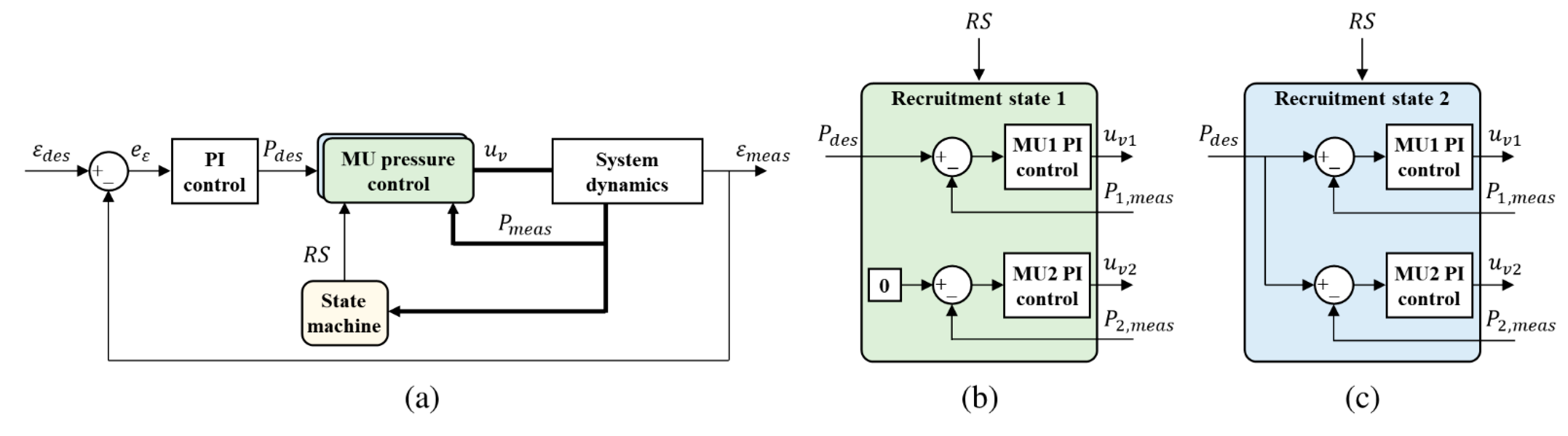
3. Controller Design

Two control schemes are presented in this section. The first control scheme is the baseline controller which uses a specified percentage of the source pressure as the threshold pressure at which a recruitment state transition is initiated. Next, the proposed control scheme is presented by its two components: pressure compensation and lag compensation. At the end of this section, the two controllers are compared by their recruitment transition logic state machines along with their control block diagrams.

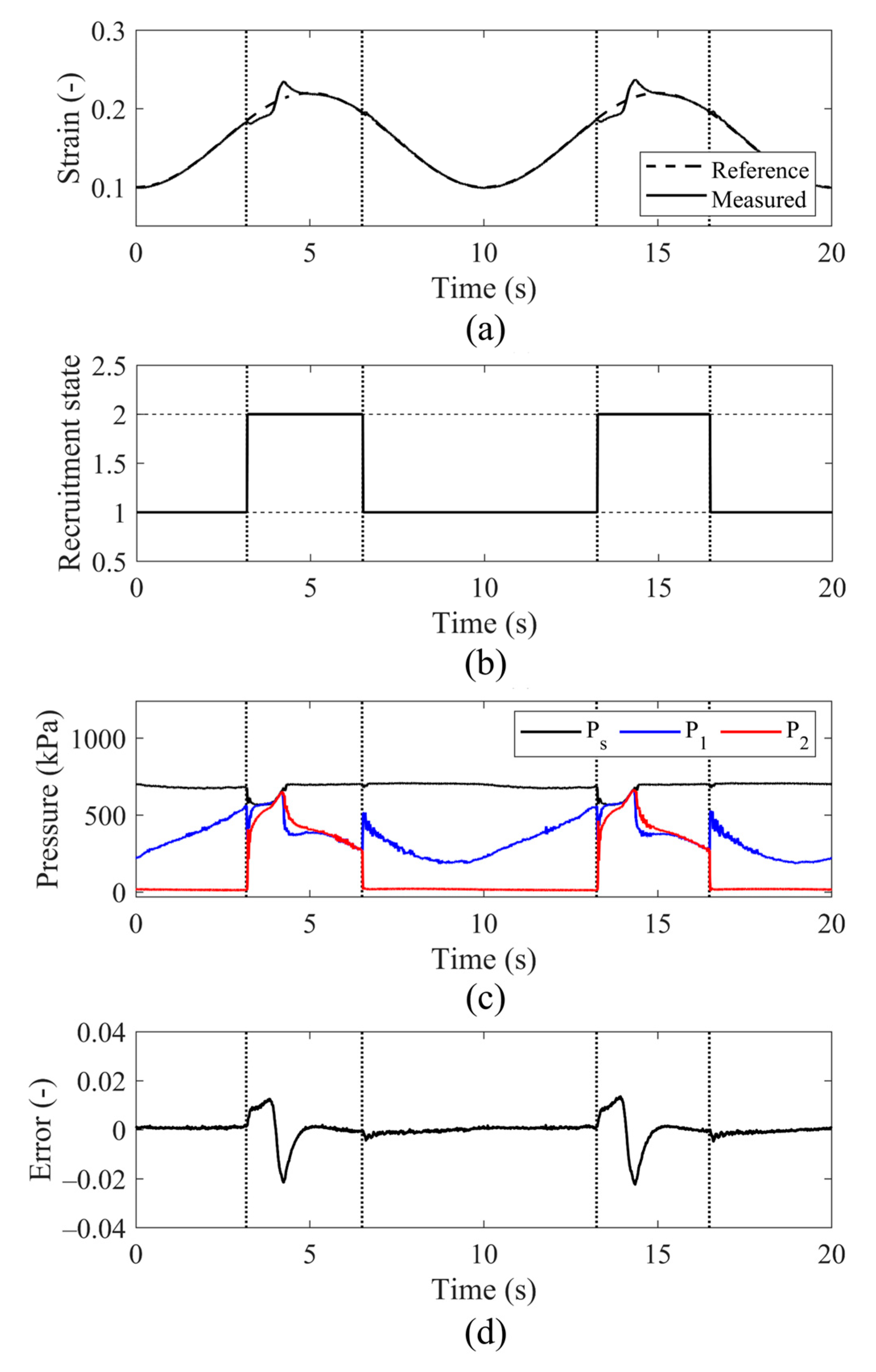
3.1. Baseline Scheme: Cascaded PI-PI Control Using Pressure Thresholds for State Transitions

The block diagram for the baseline controller is presented in Figure 3. The controller consists of a strain feedback outer PI control loop with a nested pressure feedback inner PI control loop. A cascaded PI-PI control architecture such as this one has been shown to improve the tracking performance and disturbance rejection when controlling FAMs as independent actuators [20,25]. Because the system’s pressure dynamics are fast in comparison to the strain dynamics, the gains for the inner pressure controller were tuned first and treated as part of the plant while tuning the gains for the outer strain feedback controller. The pressure measurements, $P_{meas},$ which consist of the MU1 and MU2 pressures from the system, are used to determine the recruitment state. When in RS1, the desired pressure for MU2 is simply zero. When in RS2, the same desired pressure is used to control the pressures for both MU1 and MU2, which corresponds to the batch recruitment scheme discussed in detail by Jenkins et al. [22].

The recruitment transition logic state machine for the baseline control scheme is shown in Figure 4. The default recruitment state is RS1 at startup. The recruitment upshift to RS2 occurs when MU1 pressure is greater than or equal to 80% of the nominal source pressure and downshifts when MU2 pressure is less than or equal to 40% of the nominal source pressure. These shift criteria are tuned ad hoc for a particular system, load, and trajectory.

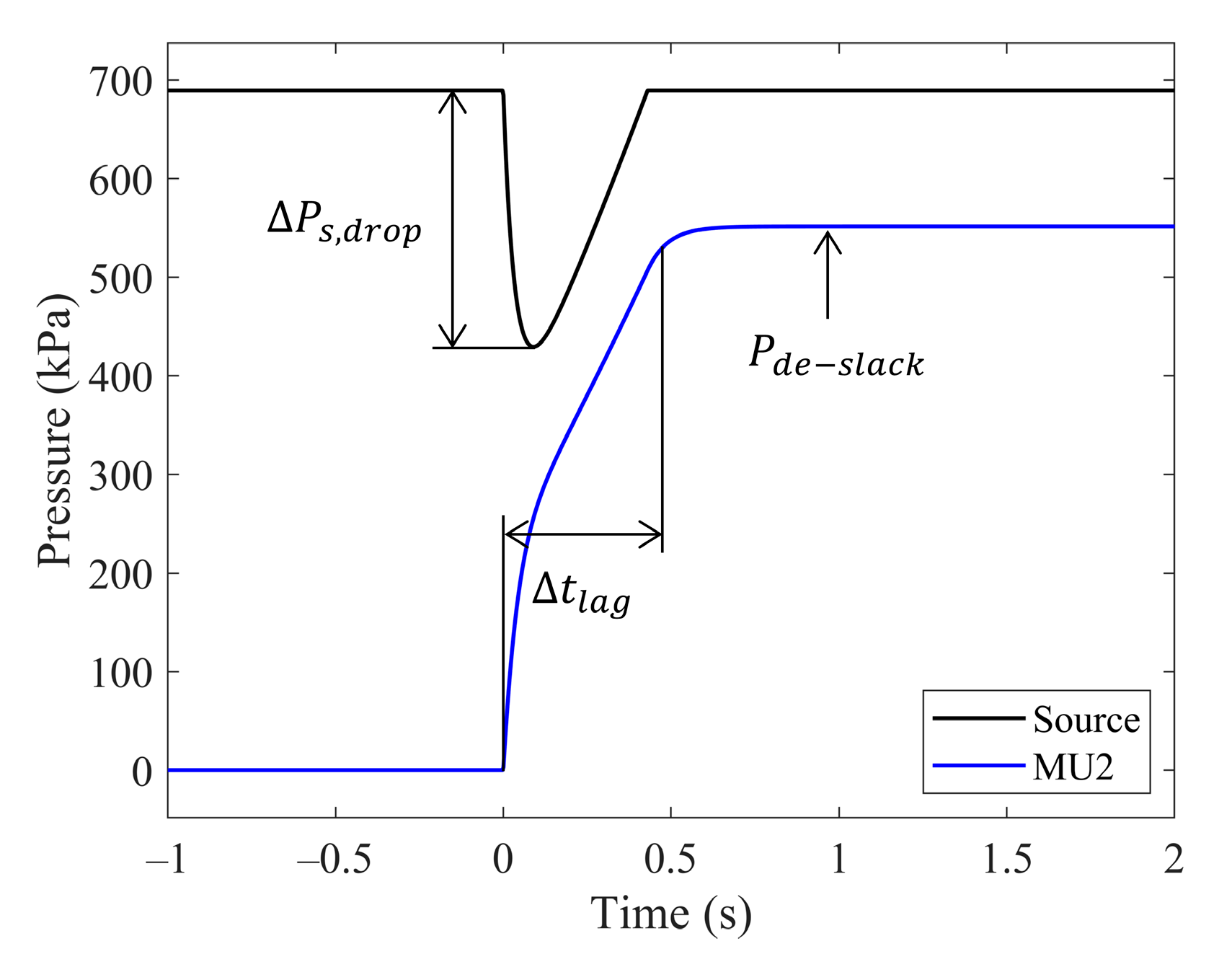
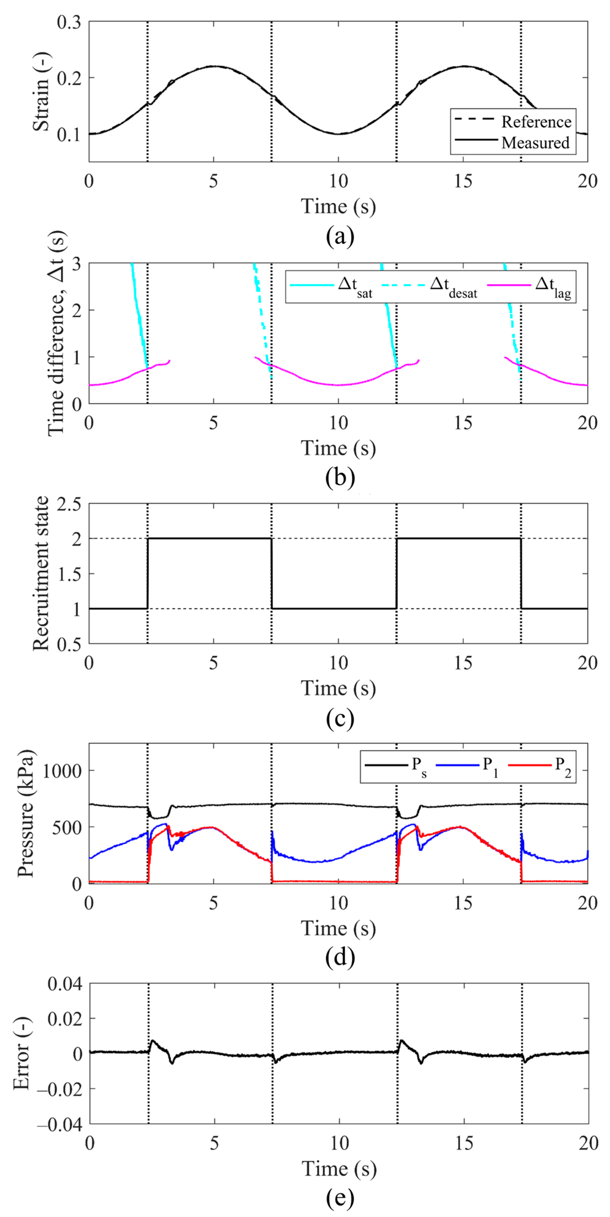
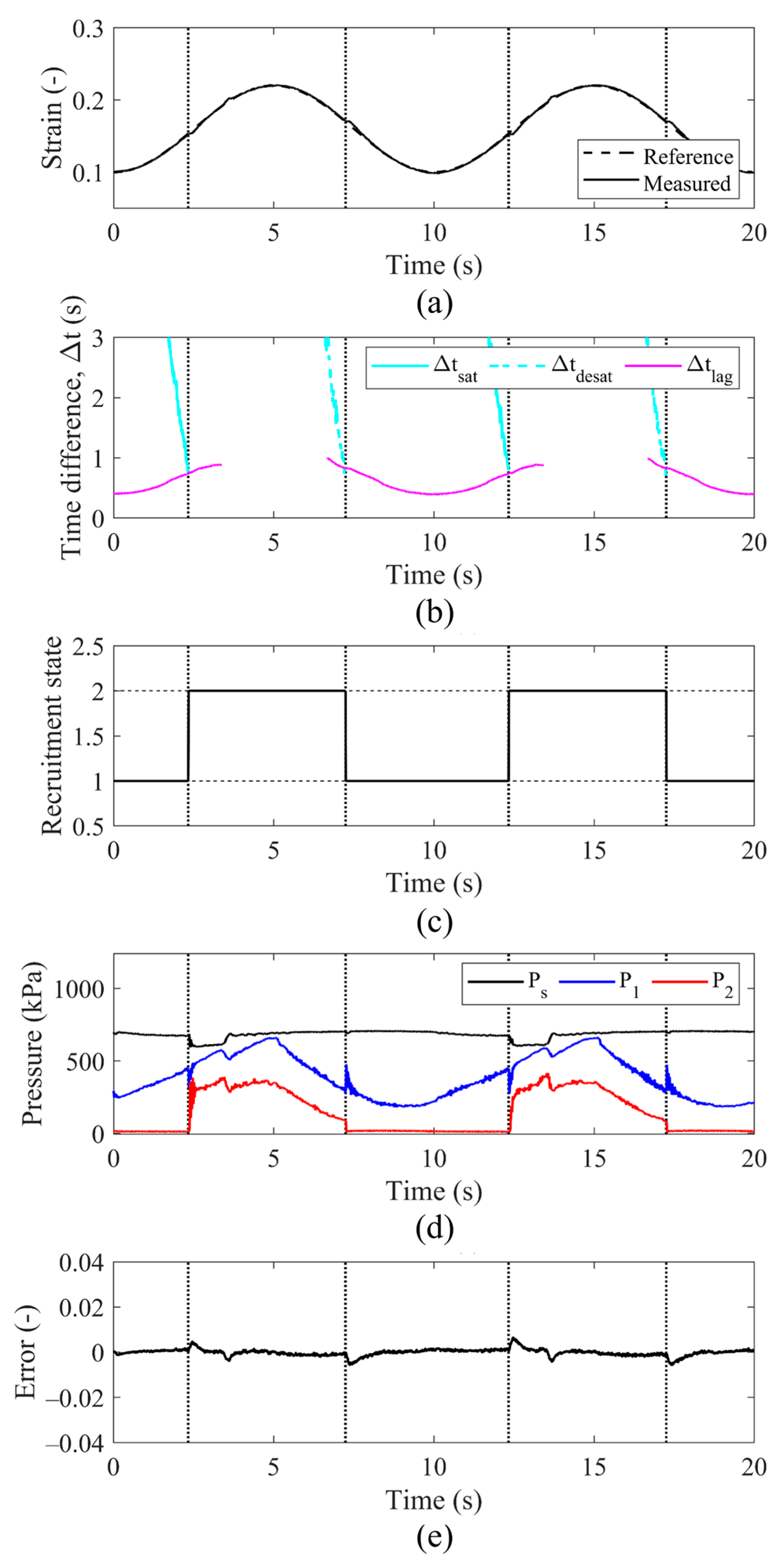
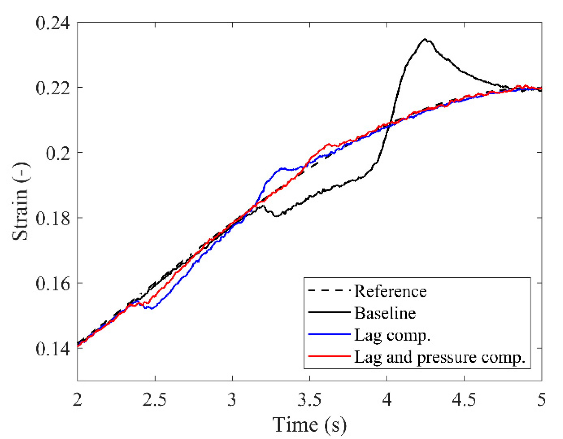
3.2. Proposed Scheme: Cascaded PI-PI Control with Lag and Pressure Compensation

The diagram for the proposed model-based controller with lag and pressure compensation is shown in Figure 5. On the high level, it has the same cascaded PI-PI control architecture with the same gains as the baseline system so as to isolate the performance change due to the model-based compensation scheme. Instead of using a preset pressure threshold, recruitment state transitions are determined through lag compensation taking into account the dynamics of the hydraulic system. Additionally, the resistive force of MU2 before it reaches the de-slack pressure is mitigated using pressure compensation by an added measured pressure feedback term.

3.2.1. Pressure Compensation

The proposed control scheme addresses the resistive effect, aforementioned in Section 2.1, which is the effect of FAMs in compression decreasing the overall force output of a variable recruitment bundle [45]. To counteract the resistive forces of inactive and newly recruited FAMs in compression, the pressure of the FAMs already in the tensile region is increase by an amount of $P_{comp}.$ First, to determine whether MU2 is in compression, the de-slack pressure is determined through a look-up table of the FAM force–strain-pressure surface that satisfies the condition:

$$F_{2,mod}\left(P_{de-slack}, {\epsilon }_{meas}\right)=0,$$

(9)

where $F_{2,mod}$ is the force of MU2 predicted by the model and ${\epsilon }_{meas}$ is the measured instantaneous strain of the bundle. It should be noted that for any MU2 pressure, $P_2$, below $P_{de-slack}$, the force of MU2 is negative. To compensate for the negative MU2 force when the measured pressure of MU2, $P_{2,meas}$, is less than $P_{de-slack}$, the MU1 force must increase by an amount equal to the resistive force of MU2 as:

$$\begin{array}{ll}{F}_{1,comp}& =F_{2,mod}\left(P_{2,meas},{\epsilon }_{meas}\right)\hfill \\ & =F_{1,mod}\left(P_{1,meas}+P_{comp},{\epsilon }_{meas}\right)-F_{MU1}\left(P_{1,meas},{\epsilon }_{meas}\right),\end{array}$$

(10)

where $F_{1,mod}$ is the force of MU1 predicted by the model, $P_{1,meas}$ is the measured pressure of MU1, and $P_{comp}$ is the amount of additional pressure required by MU1. Thus, the predicted overall force of the bundle can be expressed by:

$$F_{bundle,mod}=F_{1,mod}\left(P_{1,meas}+P_{comp}, {\epsilon }_{meas}\right)+F_{2,mod}\left(P_{2,meas},{\epsilon }_{meas}\right),$$

(11)

where $P_{comp}=0$ if MU2 no longer is in compression (i.e., $P_{2,meas}\ge P_{de-slack}$). At every instant of time, the $P_{comp}$ that satisfies (10) is determined, fed back, and added to the desired pressure of MU1.

3.2.2. Lag Compensation

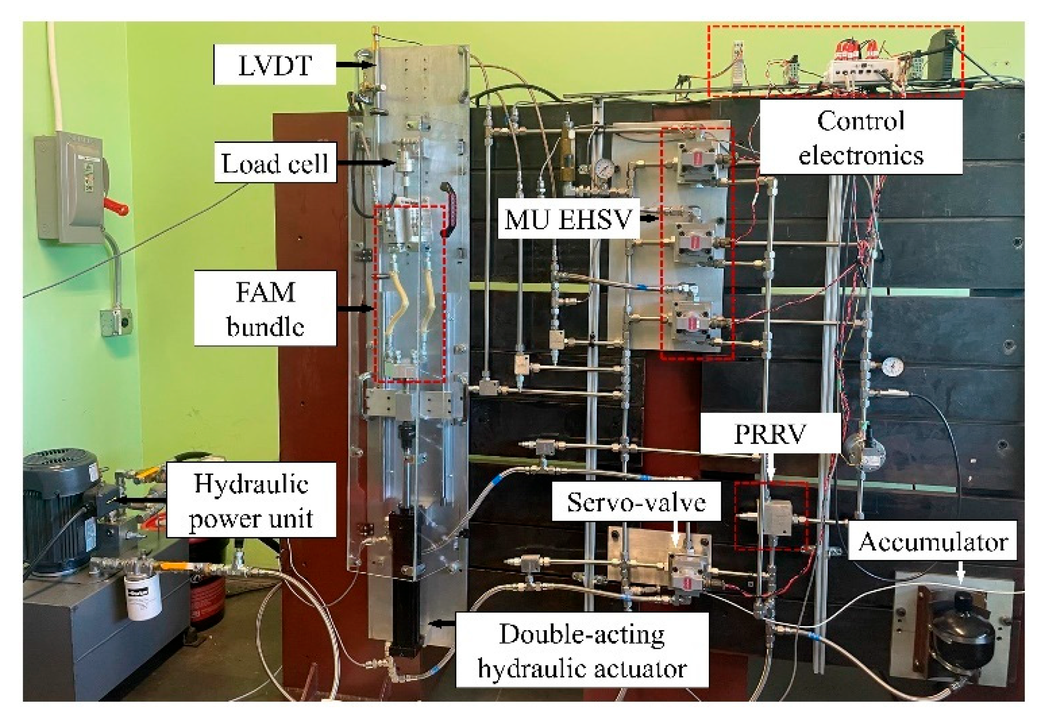
As aforementioned, the pressure dynamics of a real hydraulic system cause a lag between when the recruitment of a MU is initiated and when it reaches the de-slack pressure. This time difference is referred to as the recruitment lag, ${∆t}_{lag}$, which is defined as the time required for the pressure of a MU to reach 95% of the de-slack pressure. The recruitment lag is determined in real-time given the instantaneous source pressure and the instantaneous bundle strain using simulations of the model specified in Section 2.2. The hydraulic system model from Section 2.2 is used to simulate the pressure transients as it tracks a step reference to the de-slack pressure as shown in Figure 6. This pressure response represents the pressure applied to a MU being newly recruited during state transition.

According to the de-slack effect, the pressure of the subsequent MU being recruited must reach the de-slack pressure before it is able to contribute any positive force or strain. Additionally, while below the de-slack pressure, the recruited MU is in a buckled state and exerting a resistive force. The recruitment lag informs the controller how much in advance the state transition must begin in order to guarantee enough time before the current MU is saturated and cannot generate the force or strain required to track a desired reference. The determining factors of recruitment lag are the de-slack pressure, instantaneous source pressure, and the parameters of the hydraulic system. Once a simulation is run for a set of de-slack and source pressures, the time it takes for the pressure to reach 95% of the de-slack pressure is defined as the recruitment lag.

Another variable of interest is the maximum amount of source pressure drop, ${∆P}_{s,drop}$ that occurs during a recruitment transition. As the MU pressure increases, the required flowrate causes the source pressure to drop. Although a PRRV is used in this study, an analogous effect is observed in any fluid power source such as a motor/pump with an accumulator. This pressure drop is used to determine the pressure margin that is required for pressure compensation to occur, expressed as:

$$P_{margin}={∆P}_{s,drop}+P_{comp},$$

(12)

where both ${∆P}_{s,drop}$ and $P_{comp}$ are instantaneous values determined online based on $P_{s,meas}$, $P_{1,meas}$, $P_{2,meas}$, and ${\epsilon }_{meas}$ measured at a given instant. The pressure margin is used to define an effective source pressure, $P_{s,eff}$, expressed as:

$$P_{s,eff}=P_{s,meas}-P_{margin}.$$

(13)

Note that the pressures applied to MUs are always limited by source pressure. The pressure margin ensures that MU1 does not become saturated by the source pressure while pressure compensation is happening. In order to reduce computation during real-time control, the recruitment lag and source pressure drop are computed for the range of possible source pressures and de-slack pressures to generate a lookup table.

Once the lag associated with recruiting MU2 is determined, the time difference between the current time and when the MU1 would become saturated during upshift is estimated. This time difference is defined as time-to-saturation. During downshift, time-to-desaturation is defined as the time difference between the current time and when MU2 would no longer be required. At every instant of time, it is assumed that the bundle will continue to contract in the same direction with constant rate of contraction as illustrated in Figure 7. The expected strain trajectory, $E\left(t\right)$, is expressed as:

$$E\left(t\right)={\dot{\epsilon }}_{meas}t+{\epsilon }_{meas}$$

(14)

where ${\epsilon }_{meas}$ is the measured instantaneous strain and ${\dot{\epsilon }}_{meas}$ is its time derivative. Rearranging and solving for ${∆t}_{sat}$ by setting (14) equal to the strain at $P_{s,eff}$ and the measured instantaneous force, $F_{meas}$, gives us the equation for time-to-saturation and time-to-desaturation as:

$${∆t}_{sat}={\displaystyle \frac{{\epsilon }_{mod}\left(P_{s,eff}, F_{meas}\right)-{\epsilon }_{meas}}{{\dot{\epsilon }}_{meas}}},$$

(15)

and

$${∆t}_{desat}={\displaystyle \frac{{\epsilon }_{mod}\left(P_{s,meas}, F_{meas}\right)-{\epsilon }_{meas}}{{\dot{\epsilon }}_{meas}}}.$$

(16)

where ${\epsilon }_{mod}$ is the bundle strain predicted by the model. Note that $E\left(t\right)$ can be generalized to other forms of expected trajectories such as a sinusoid instead of the linear assumption used in this study. This would be useful if some knowledge about the control application was given in advance.

For the proposed model-based control scheme, the state transition decision is made through time-to-saturation, time-to-desaturation, and recruitment lag conditions as shown in Figure 8. Note that the recruitment lag is an estimation of the time it takes for a newly recruited MU to de-slack and begin to positively contribute to overall bundle output. Time-to-saturation is an estimate of how long in advance the bundle will require the newly recruited MU to provide additional force. Thus, the state transition must occur when the time-to-saturation is less than or equal to the recruitment lag in order to ensure that the bundle is provided with the force of the newly recruited MU in time. Note that, from an efficiency perspective, it is advantageous for a variable recruitment bundle to operate at the lowest recruitment state possible. This allows the applied pressures to the activated MUs to be closest to the source pressure, thus allowing the bundle to operate more efficiently by minimizing throttling energy losses. However, higher recruitment states provide better control authority. Therefore, properly deciding when to initiate a recruitment state transition is important for operating a variable recruitment bundle efficiently and with satisfactory tracking performance. The lag compensation method proposed in this study provides an online method of estimating that time based on information from the model and the measured states.

4. Experiment Setup

FAMs were constructed using silicone tubing with a Shore hardness value of A50 and a double-helix braided Kevlar mesh. A neoprene spacer was placed over the mesh at each end and crimped using a hydraulic press. The FAM assembly method was identical to that of detailed in Meller et al., 2014 [48]. FAM dimensions and specifications are summarized in

Table 1. FAM dimensions and specifications.

FAM dimensions	Initial inner radius $\left(\mathrm{m}\right)$	$r_0$	0.0063
	Initial thickness $\left(\mathrm{m}\right)$	$t_0$	0.0016
	Initial braid angle $\left(°\right)$	${\alpha }_0$	33
	Initial length $\left(\mathrm{m}\right)$	$L_0$	0.222
Empirical-based tuning correction factors	Young’s modulus	-	1.3
	Collapse moment	-	0.75
	Torsional spring constant	-	0.9P + 1.54
	Transition constant	$\beta$	100

. The force–strain relationship was then corrected using empirical-based correction factors, for which the details can be found in [45]. Experiments were carried out on the linear hydraulic actuator characterization device (LHACD) shown in Figure 9, which was developed in-house by Chipka et al. in 2017 [49]. The LHACD consisted of a $3.73 \mathrm{k}\mathrm{W}\left(5\mathrm{h}\mathrm{p}\right)$ hydraulic power unit (Concentric GC9500, Stockholm, Sweden) capable of producing pressures up to $1.03\times {10}^4 \mathrm{k}\mathrm{P}\mathrm{a}\left(1500 \mathrm{p}\mathrm{s}\mathrm{i}\right)$ at a rated flow of $3.78 {\mathrm{m}}^3/\mathrm{s}\left(6 \mathrm{g}\mathrm{p}\mathrm{m}\right)$. A pressure reducing/relief valve (PRRV) from Sun Hydraulics (PRDV-LEV, Sarasota, FL, USA) was used to regulate the downstream circuit nominal source pressure down to $689.5 \mathrm{k}\mathrm{P}\mathrm{a}\left(100 \mathrm{p}\mathrm{s}\mathrm{i}\right)$ for the safe operation of FAMs without rupturing. The regulated pressure output of a PRRV is dependent on the rate of fluid flow through the valve, which is provided by the manufacturer for several values of operating pressure. For a source pressure of $689.5 \mathrm{k}\mathrm{P}\mathrm{a}\left(100 \mathrm{p}\mathrm{s}\mathrm{i}\right)$, the pressure–flowrate relationship is experimentally determined, for which the results are shown in Figure 10. It should be noted that for cases when the pressure output of the PRRV exceeds the set value of $\mathrm{6.89.5} \mathrm{k}\mathrm{P}\mathrm{a}\left(100 \mathrm{p}\mathrm{s}\mathrm{i}\right)$, its relieving function is engaged, and fluid is directed to the reservoir instead of the downstream circuit. Located downstream of the PRRV were two four-way directional servo valves (MOOG G761, Elma, NY, USA) that were used to control the pressures of the two MUs. Pressure transducers (TE MP300, Berwyn, PA, USA) were installed to measure the source pressure and the two pressures downstream of each servo valve. A flowmeter (Omega FPD2003, Norwalk, CT, USA) was installed to measure the flowrate of the PRRV output. A linear variable differential transducer (LVDT) by the RDP group (DR7AC, Dayton, OH, USA) was used to measure the contraction of the FAM bundle. Lastly, servo valve control and data acquisition were performed using a Quanser QPID I/O board (Markham, ON, Canada). All data were acquired at a sampling rate of 1000 Hz without any frequency filters.

5. Results

The performance of the baseline controller with state transitions based on pressure thresholds (Figure 11), controller with lag compensation only (Figure 12), and controller with both lag and pressure compensation (Figure 13) are presented in this section. For all control scheme cases, a sinusoidal reference trajectory with a frequency of 0.1 Hz and a strain amplitude of 0.06 is specified. A mass of 18.8 kg was hung from the bottom of the FAM bundle.

For the system with the baseline controller, the position tracking performance is shown in Figure 11a. The source pressure and the pressures applied to MU1 and MU2 are shown in Figure 11c. According to the state machine shown in Figure 6, the upshift to recruitment state 2 is made once the MU1 pressure reaches $551.6 \mathrm{k}\mathrm{P}\mathrm{a}\left(80 \mathrm{p}\mathrm{s}\mathrm{i}\right)$, which is 80% of the nominal source pressure. Recruitment state is shifted down at 40% of the nominal source pressure. The recruitment shift is depicted in all subfigures as a vertical dashed line. Immediately after state upshift, the strain lags further behind the reference strain, which results in overshoot, as the controller attempts to compensate for the error due to lag. The lag is mainly attributed to the saturation of MU1 pressure, as only pressures as high as the instantaneous source pressure can be applied to the MUs. As expected from simulation predictions (e.g., Figure 6), the recruitment of MU2 causes a drop in source that further limits the MU1 pressure.

The experimental results for the controller with lag compensation applied are shown in Figure 12. The time-to-saturation, time-to-desaturation, and the recruitment lag were determined at every instant of time, as shown in Figure 12b. As the bundle strain tracked the reference, the time-to-saturation decreased as the bundle came closer to the time at which the recruitment state transition must occur. Simultaneously, the recruitment lag, according to the instantaneous source pressure and de-slack pressure of MU2, increased with increasing strain. The time at which recruitment state transition occurred was determined when the time-to-saturation dropped below the recruitment lag, as demonstrated by Figure 12b,c. As a result, the state upshift occurred earlier compared to the baseline controller case, thus allowing the necessary pressure of MU1 to be applied without being saturated, as shown in Figure 12d. Consequently, the strain lag immediately following a state transition was significantly reduced. The argument can be made that the same effect can be achieved by lowering the pressure threshold of the baseline case. However, a certain pressure threshold is effective only for a trajectory with a specific range of amplitudes and frequencies, and thus, is only useful if the reference trajectory is known in advance. Additionally, the pressure threshold may need to be determined empirically. By determining the time-to-saturation and recruitment lag based on the instantaneous measured states during control, the proposed controller provides an online method of determining when the state transition must occur real-time.

The tracking performance can be further increased by applying pressure compensation in addition to lag compensation as shown in Figure 13. The pressure feedback term provides anticipatory information on what the pressure of MU1 should be based on the resistive force of MU2. The state transition occurs based on lag compensation. The effect of pressure compensation is evident in MU1 pressure after the state shift, as shown by Figure 13d. The improved tracking performance is better demonstrated by a zoomed-in view of the measured strains for all cases in Figure 14. The integral absolute error (IAE) for strain for one cycle and the maximum strain error is determined by:

$${IAE}_{\epsilon }=\int \left|{\epsilon }_{ref}-{\epsilon }_{meas}\right|dt,$$

(17)

where ${\epsilon }_{ref}$ is the reference strain and ${\epsilon }_{meas}$ is the measured strain. The maximum strain error, ${err}_{\epsilon ,max}$, is expressed as:

$${err}_{\epsilon ,max}=max\left(\left|{\epsilon }_{ref}-{\epsilon }_{meas}\right|\right).$$

(18)

A comparison of these values is shown in

Table 2. Comparison of integrated absolute error for strain, and maximum strain error.

	Strain IAE	Max. Strain Error
Baseline controller	0.0454	0.0223
Cascaded controller with only lag compensation	0.0234	0.0075
Cascaded controller with lag and pressure compensation	0.0211	0.0064

. It should be noted that pressure compensation alone was not tested. The purpose of pressure compensation is to increase the pressure of MU1 to account for tracking errors that occur during recruitment state transitions. For pressure compensation to be possible, there needs to be an excess of source pressure from which the first MU can draw pressure from. As can be seen in Figure 11, as soon as recruitment transition happens, the MU1 pressure increases to the highest it can, which is the source pressure. Therefore, it would not be able to compensate for the tracking error by increasing MU1 pressure. Only when lag compensation is applied does the source pressure allow for MU1 pressure to increase.

6. Conclusions

This study experimentally evaluates the tracking performance of a model-based controller for state transitions of a variable recruitment FAM bundle. During variable recruitment operation, inactive/low-pressure FAMs are buckled and exert resistive forces that decrease the overall force of the bundle. This resistive effect is captured using an FAM model that predicts the axial force of FAMs beyond their free strain. A pressure feedback term is used to compensate for the decrease in force. Additionally, a hydraulic dynamics system model is used to predict the time required for a newly recruited MU that is buckled to de-slack, coined the recruitment lag. The measured strain, strain rate, pressure, and force are used to predict the time-to-saturation and time-to-desaturation. These two variables in tandem inform the control when to initiate a state transition. The proposed controller is compared to a baseline for which a pressure threshold based on a percentage of the nominal source pressure is used to initiate state transitions. A sinusoidal strain trajectory is tracked, and the measured strain is presented, along with the source pressure and MU1 and MU2 pressures. The controller showed its ability to determine the state transitions timing so that MU1 pressure is not saturated when the next MU is newly recruited. The IAE and maximum strain errors are presented to show the improved tracking performance of the proposed controller. For the purposes of this study, the linear estimation methods used in lag compensation were sufficient. If more advanced estimation methods could be applied, the proposed control scheme has the potential to be used for complex non-cyclic trajectories. Another area for future investigation is the correlation between state transition timings and actuator hydraulic efficiencies.

References

1. Tondu, B.; Lopez, P. Modelling and Control of McKibben Artificial Muscle Robot Actuators. IEEE Control. Syst. 2000, 20, 15–38. [Google Scholar] [CrossRef]
2. Tondu, B. Modelling of the McKibben artificial muscle: A review. J. Intell. Mater. Syst. Struct. 2012, 23, 225–253. [Google Scholar] [CrossRef]
3. Al-Fahaam, H.; Davis, S.; Nefti-Meziani, S. The design and mathematical modelling of novel extensor bending pneumatic artificial muscles (EBPAMs) for soft exoskeletons. Robot. Auton. Syst. 2017, 99, 63–74. [Google Scholar] [CrossRef]
4. Xiao, W.; Hu, D.; Chen, W.; Yang, G.; Han, X. Modeling and analysis of bending pneumatic artificial muscle with multi-degree of freedom. Smart Mater. Struct. 2021, 30, 095018. [Google Scholar] [CrossRef]
5. Zou, J.; Feng, M.; Ding, N.; Yan, P.; Xu, H.; Yang, D.; Fang, N.X.; Gu, G.; Zhu, X. Muscle-fiber array inspired, multiple-mode, pneumatic artificial muscles through planar design and one-step rolling fabrication. Natl. Sci. Rev. 2021, 8, nwab048. [Google Scholar] [CrossRef]
6. Phan, P.T.; Hoang, T.T.; Thai, M.T.; Low, H.; Lovell, N.H.; Do, T.N. Twisting and Braiding Fluid-Driven Soft Artificial Muscle Fibers for Robotic Applications. Soft Robot. 2022, 9, 820–836. [Google Scholar] [CrossRef]
7. Wirekoh, J.; Valle, L.; Pol, N.; Park, Y.-L. Sensorized, Flat, Pneumatic Artificial Muscle Embedded with Biomimetic Microfluidic Sensors for Proprioceptive Feedback. Soft Robot. 2019, 6, 768–777. [Google Scholar] [CrossRef]
8. Yang, H.D.; Greczek, B.T.; Asbeck, A.T. Modeling and analysis of a high-displacement pneumatic artificial muscle with integrated sensing. Front. Robot. AI 2019, 5, 136. [Google Scholar] [CrossRef]
9. Tiziani, L.O.; Hammond, F.L. Optical Sensor-Embedded Pneumatic Artificial Muscle for Position and Force Estimation. Soft Robot. 2020, 7, 462–477. [Google Scholar] [CrossRef]
10. Legrand, J.; Loenders, B.; Vos, A.; Schoevaerdts, L.; Poorten, E.V. Integrated Capacitance Sensing for Miniature Artificial Muscle Actuators. IEEE Sens. J. 2020, 20, 1363–1372. [Google Scholar] [CrossRef]
11. Jenkins, T.; Bryant, M. Pennate actuators: Force, contraction and stiffness. Bioinspiration Biomim. 2020, 15, 046005. [Google Scholar] [CrossRef] [PubMed]
12. Duan, E.; Bryant, M. Implications of Spatially Constrained Bipennate Topology on Fluidic Artificial Muscle Bundle Actuation. Actuators 2022, 11, 82. [Google Scholar] [CrossRef]
13. Andrikopoulos, G.; Nikolakopoulos, G.; Manesis, S. A Survey on applications of Pneumatic Artificial Muscles. In Proceedings of the 2011 19th Mediterranean Conference on Control and Automation, MED 2011, Corfu, Greece, 20–23 June 2011; pp. 1439–1446. [Google Scholar] [CrossRef]
14. Ogawa, K.; Thakur, C.; Ikeda, T.; Tsuji, T.; Kurita, Y. Development of a pneumatic artificial muscle driven by low pressure and its application to the unplugged powered suit. Adv. Robot. 2017, 31, 1135–1143. [Google Scholar] [CrossRef]
15. Pawar, M.V. Experimental Modelling of Pneumatic Artificial Muscle Systems Designing of Prosthetic Robotic Arm. In Proceedings of the 2018 3rd International Conference for Convergence in Technology (I2CT), I2CT 2018, Pune, India, 6–8 April 2018; pp. 18–23. [Google Scholar] [CrossRef]
16. Choi, H.S.; Lee, C.H.; Baek, Y.S. Design and Validation of a Two-Degree-of-Freedom Powered Ankle-Foot Orthosis with Two Pneumatic Artificial Muscles. Mechatronics 2020, 72, 102469. [Google Scholar] [CrossRef]
17. Henneman, E.; Somjen, G.; Carpenter, D.O. Excitability and inhibitibility of motoneurons of different sizes. J. Neurophysiol. 1965, 28, 599–620. [Google Scholar] [CrossRef]
18. Bryant, M.; Meller, M.A.; Garcia, E. Variable recruitment fluidic artificial muscles: Modeling and experiments. Smart Mater. Struct. 2014, 23, 074009. [Google Scholar] [CrossRef]
19. Jenkins, T.E.; Chapman, E.M.; Bryant, M. Bio-inspired online variable recruitment control of fluidic artificial muscles. Smart Mater. Struct. 2016, 25, 125016. [Google Scholar] [CrossRef]
20. Robinson, R.M.; Kothera, C.S.; Wereley, N.M. Variable Recruitment Testing of Pneumatic Artificial Muscles for Robotic Manipulators. IEEE/ASME Trans. Mechatron. 2014, 20, 1642–1652. [Google Scholar] [CrossRef]
21. Delahunt, S.A.; Pillsbury, T.E.; Wereley, N.M. Variable recruitment in bundles of miniature pneumatic artificial muscles. Bioinspiration Biomim. 2016, 11, 056014. [Google Scholar] [CrossRef]
22. Chapman, E.M.; Jenkins, T.; Bryant, M. Design and Analysis of Electrohydraulic Pressure Systems for Variable Recruitment in Fluidic Artificial Muscles. Smart Mater. Struct. 2018, 27, 105024. [Google Scholar] [CrossRef]
23. Mazzoleni, N.; Kim, J.Y.; Bryant, M. Motor unit buckling in variable recruitment fluidic artificial muscle bundles: Implications and mitigations. Smart Mater. Struct. 2022, 31, 035004. [Google Scholar] [CrossRef]
24. Focchi, M.; Guglielmino, E.; Semini, C.; Parmiggiani, A.; Tsagarakis, N.; Vanderborght, B.; Caldwell, D.G. Water/air performance analysis of a fluidic muscle. In Proceedings of the 2010 IEEE/RSJ International Conference on Intelligent Robots and Systems (IROS 2010), Taipei, Taiwan, 18–22 October 2010; pp. 2194–2199. [Google Scholar] [CrossRef]
25. Minh, T.V.; Tjahjowidodo, T.; Ramon, H.; Van Brussel, H. Cascade position control of a single pneumatic artificial muscle–mass system with hysteresis compensation. Mechatronics 2010, 20, 402–414. [Google Scholar] [CrossRef]
26. Ganguly, S.; Garg, A.; Pasricha, A.; Dwivedy, S. Control of pneumatic artificial muscle system through experimental modelling. Mechatronics 2012, 22, 1135–1147. [Google Scholar] [CrossRef]
27. Ba, D.X.; Dinh, T.Q.; Ahn, K.K. An Integrated Intelligent Nonlinear Control Method for a Pneumatic Artificial Muscle. IEEE/ASME Trans. Mechatron. 2016, 21, 1835–1845. [Google Scholar] [CrossRef]
28. Zhang, Z.; Philen, M. Pressurized artificial muscles. J. Intell. Mater. Syst. Struct. 2011, 23, 255–268. [Google Scholar] [CrossRef]
29. Ai, Q.; Ke, D.; Zuo, J.; Meng, W.; Liu, Q.; Zhang, Z.; Xie, S.Q. High-Order Model-Free Adaptive Iterative Learning Control of Pneumatic Artificial Muscle with Enhanced Convergence. IEEE Trans. Ind. Electron. 2019, 67, 9548–9559. [Google Scholar] [CrossRef]
30. Sun, N.; Liang, D.; Wu, Y.; Chen, Y.; Qin, Y.; Fang, Y. Adaptive Control for Pneumatic Artificial Muscle Systems with Parametric Uncertainties and Unidirectional Input Constraints. IEEE Trans. Ind. Inform. 2019, 16, 969–979. [Google Scholar] [CrossRef]
31. Duong, M.-D.; Pham, Q.-T.; Vu, T.-C.; Bui, N.-T.; Dao, Q.-T. Adaptive fuzzy sliding mode control of an actuator powered by two opposing pneumatic artificial muscles. Sci. Rep. 2023, 13, 8242. [Google Scholar] [CrossRef]
32. Nguyen, V.-T.; Pham, B.-L.; Nguyen, T.-V.; Bui, N.-T.; Dao, Q.-T. Sliding mode control of antagonistically coupled pneumatic artificial muscles using radial basis neural network function. SN Appl. Sci. 2023, 5, 246. [Google Scholar] [CrossRef]
33. Zhao, Z.; Hao, L.; Tao, G.; Liu, H.; Shen, L. Prescribed performance sliding mode control for the PAMs elbow exoskeleton in the tracking trajectory task. Ind. Robot. 2023, 51, 167–176. [Google Scholar] [CrossRef]
34. Lin, C.-J.; Sie, T.-Y. Design and Experimental Characterization of Artificial Neural Network Controller for a Lower Limb Robotic Exoskeleton. Actuators 2023, 12, 55. [Google Scholar] [CrossRef]
35. Meller, M.; Chipka, J.; Volkov, A.; Bryant, M.; Garcia, E. Improving actuation efficiency through variable recruitment hydraulic McKibben muscles: Modeling, orderly recruitment control, and experiments. Bioinspir. Biomim. 2016, 11, 065004. [Google Scholar] [CrossRef] [PubMed]
36. Kulkarni, M.; Shim, T.; Zhang, Y. Shift dynamics and control of dual-clutch transmissions. Mech. Mach. Theory 2006, 42, 168–182. [Google Scholar] [CrossRef]
37. Kahlbau, S.; Bestle, D. Optimal shift control for automatic transmission. Mech. Based Des. Struct. Mach. 2013, 41, 259–273. [Google Scholar] [CrossRef]
38. Kuo, K.L. Simulation and analysis of the shift process for an automatic transmission. World Acad. Sci. Eng. Technol. 2011, 76, 341–347. [Google Scholar]
39. Walker, P.; Zhu, B.; Zhang, N. Powertrain dynamics and control of a two speed dual clutch transmission for electric vehicles. Mech. Syst. Signal Process. 2017, 85, 1–15. [Google Scholar] [CrossRef]
40. Zhang, Q.; Liu, X. Optimization of the Quality of the Automatic Transmission Shift and the Power Transmission Characteristics. Energies 2022, 15, 4672. [Google Scholar] [CrossRef]
41. Chou, C.-P.; Hannaford, B. Measurement and modeling of McKibben pneumatic artificial muscles. IEEE Trans. Robot. Autom. 1996, 12, 90–102. [Google Scholar] [CrossRef]
42. Sangian, D.; Naficy, S.; Spinks, G.M.; Tondu, B. The effect of geometry and material properties on the performance of a small hydraulic McKibben muscle system. Sens. Actuators A Phys. 2015, 234, 150–157. [Google Scholar] [CrossRef]
43. Yu, Z.; Pillsbury, T.; Wang, G.; Wereley, N.M. Hyperelastic analysis of pneumatic artificial muscle with filament-wound sleeve and coated outer layer. Smart Mater. Struct. 2019, 28, 105019. [Google Scholar] [CrossRef]
44. Kalita, B.; Leonessa, A.; Dwivedy, S.K. A Review on the Development of Pneumatic Artificial Muscle Actuators: Force Model and Application. Actuators 2022, 11, 288. [Google Scholar] [CrossRef]
45. Kim, J.Y.; Mazzoleni, N.; Bryant, M. Modeling of Resistive Forces and Buckling Behavior in Variable Recruitment Fluidic Artificial Muscle Bundles. Actuators 2021, 10, 42. [Google Scholar] [CrossRef]
46. Klute, G.K.; Hannaford, B. Accounting for Elastic Energy Storage in McKibben Artificial Muscle Actuators. J. Dyn. Syst. Meas. Control. 1998, 122, 386–388. [Google Scholar] [CrossRef]
47. Jelali, M.; Kroll, A. Hydraulic Servo-Systems: Modeling, Identification and Control; Springer: London, UK, 2003. [Google Scholar]
48. Meller, M.A.; Bryant, M.; Garcia, E. Reconsidering the McKibben muscle: Energetics, operating fluid, and bladder material. J. Intell. Mater. Syst. Struct. 2014, 25, 2276–2293. [Google Scholar] [CrossRef]
49. Chipka, J.; Meller, M.A.; Volkov, A.; Bryant, M.; Garcia, E. Linear dynamometer testing of hydraulic artificial muscles with variable recruitment. J. Intell. Mater. Syst. Struct. 2017, 28, 2051–2063. [Google Scholar] [CrossRef]
Figure 1. Variable recruitment fluidic artificial muscle (FAM) bundle with two motor units (MUs), each consisting of two FAMs in the (a) inactive resting state, (b) first recruitment state showing buckling of inactive/low-pressure FAMs, and (c) second recruitment state with all MUs fully active.
Actuators 14 00235 g001
Figure 2. Diagram of the hydraulic system.
Actuators 14 00235 g002
Figure 3. Block diagram of the baseline controller with pressure thresholds. (a) High-level diagram showing the outer strain feedback control loop and plant. The inner pressure feedback control loops which are dependent on the recruitment state are shown for (b) recruitment state 1 and (c) recruitment state 2. The state machine block is shown in Figure 4. Bold lines represent vectors with two elements corresponding to the two MUs.
Actuators 14 00235 g003
Figure 4. State machine with two MUs for the baseline controller with recruitment pressure thresholds.
Actuators 14 00235 g004
Figure 5. Block diagram of the proposed controller with lag and pressure compensation. (a) The high-level diagram showing the outer strain feedback control loop and plant. The inner pressure feedback control loops which are dependent on the recruitment state are shown for (b) recruitment state 1 and (c) recruitment state 2. Bold lines represent vectors with two elements corresponding to the two MUs.
Actuators 14 00235 g005
Figure 6. Example simulation of hydraulic system pressure dynamics for a nominal source pressure of 689.5   k P a 100   p s i and a de-slack pressure of 551.6   k P a 80   p s i . The recruitment lag, t l a g , which is defined as the time required to reach 95% of the de-slack pressure and the maximum source pressure drop, P s ,   d r o p , is determined.
Actuators 14 00235 g006
Figure 7. Example determination of time-to-saturation, t s a t , time-to-desaturation, t d e s a t .
Actuators 14 00235 g007
Figure 8. State machine with two MUs for the proposed controller using lag compensation to shift between states.
Actuators 14 00235 g008
Figure 9. The linear hydraulic actuator characterization device (LHACD) used for experiments in this study.
Actuators 14 00235 g009
Figure 10. Pressure–flowrate relationship of the PRRV. Measured values are indicated in black markers. The linear line fit used for simulations is shown in solid black line.
Actuators 14 00235 g010
Figure 11. Experimental results of cascaded controller with state transitions using pressure thresholds. (a) Position tracking; (b) recruitment state; (c) pressures for source, MU1, and MU2; (d) strain tracking error.
Actuators 14 00235 g011
Figure 12. Experimental results of cascaded controller with state transitions with lag compensation applied. (a) Position tracking; (b) time-to-saturation, time-to-desaturation, and recruitment lag; (c) recruitment state; (d) pressures for source, MU1, and MU2; (e) strain tracking error.
Actuators 14 00235 g012
Figure 13. Experimental results of cascaded controller with state transitions with lag compensation and pressure compensation applied. (a) Position tracking; (b) time-to-saturation, time-to-desaturation, and recruitment lag; (c) recruitment state; (d) pressures for source, MU1, and MU2; (e) strain tracking error.
Actuators 14 00235 g013
Figure 14. Reference and measured strain immediately following recruitment state transition of baseline and proposed controllers.
Actuators 14 00235 g014