Article

Three-Dimensional Modelling and Validation for the Ultra-High-Speed EDS Rocket Sled with PM Halbach Array

by
Yongpan Hu
1,*,
Baojun Chen
2,
Guobin Lin
1 and
Zhiqiang Wang
2
1
Key Laboratory of Railway Industry of Maglev Technology, College of Transportation, Tongji University, Shanghai 201804, China
2
College of Intelligence Science and Technology, National University of Defense Technology, Changsha 410073, China
*
Author to whom correspondence should be addressed.
Actuators 2025, 14(5), 225; https://doi.org/10.3390/act14050225
Submission received: 1 April 2025 / Revised: 22 April 2025 / Accepted: 29 April 2025 / Published: 1 May 2025
(This article belongs to the Special Issue Advanced Theory and Application of Magnetic Actuators—2nd Edition)

Abstract

:
The ultra-high-speed rocket sled plays an important role in the ground test by simulating altitude flight. Rocket sleds can only be lifted for a short time with thermally uninsulated superconductors moving among an eddy-current-induced copper array. For the purpose of durable lifting, an electrodynamic suspension (EDS) with a permanent magnet (PM) Halbach array moving over a conductor plate can be adopted to upgrade the rocket sled. The earlier study built a two-dimensional (2D) model for the PM EDS system. Yet, 2D modelling in our earlier research ignored the magnetic field variation along both widths of the Halbach array and conductor plate. This resulted in a more than 50% error between the analytical electromagnetic forces with both the three-dimensional (3D) simulated and experimental results. To reduce the error, this paper puts forward more accurate analytical electromagnetic force formulas by a 3D modelling method encompassing both widths of the Halbach array and conductor plate. The 3D model was built by periodically extending the PM EDS system along both directions of the width and length. Then, by double Fourier series expansion and omitting high-order components, the electromagnetic forces can be approximated by brief formulas. Moreover, lift-to-weight and lift-to-drag optimization are discussed. Finally, the correctness of the 3D electromagnetic force formulas was verified by both the numerical simulation and experiment.

1. Introduction

The ultra-high-speed rocket sled test can reproduce the supersonic flight environment on the ground, which is conducive to conduct aircraft performance, high-speed life-saving, and high-speed collision tests. In the early stage, the rocket sled held the track on by two pairs of metal sliding shoes. When the rocket engine pushes the rocket skid, the sliding shoes touch the track directly, causing a gouging [1,2], and the sliding shoes were hardly reused. In addition, the high-strength vibration of the rocket sled caused by the mechanical friction seriously affected the test effect [3,4]. In order to avoid gouging and reduce the vibration, the sled was upgraded by attaching superconducting coils to the bottom [5,6] and was lifted by the induced eddy currents in four copper plate. However, the superconductivity of the superconductor without insulation in the air cannot be kept long. As a result, the sled could be lifted for such a short time that it would not be accelerated to a higher speed. To overcome this shortcoming, the permanent magnet (PM) Halbach array is a promising substitute for the superconducting coil. The PM Halbach array comprises an array of regularly magnetized permanent magnets. The magnetic field concentrating on one side [7] enables it to be used in so many domains, such as permanent magnetic motor [8,9], maglev car/train [10,11,12], and electromagnetic actuator [13]. When moving above a conductor plate or laminated coils, the Halbach array interacting with induced eddy currents will produce lift force [14]. The conductor plate is easy to maintain, and the paper chooses the conductor plate as a research object. Moreover, benefitting from the former research of the MIT Hyperloop [15], the PM Halbach array–conductor plate is expected to also be used in the ultra-high-speed rocket sled.
Two modelling methods has been applied on the PM Halbach array–conductor plate system. The difference between the two methods focuses mainly on how to deal with the Halbach array. The one method adopted by [16,17,18,19,20,21] delt the Halbach array by surface currents considering its finite length. The other method shown in [22] used the Fourier series expansion by regarding the Halbach array as infinite long (that is, neglecting the edge effect). The former one has an advantage in its accuracy of calculation, while the latter one is much more meaningful in revealing the changing rule of electromagnetic force varied by structural parameters. Thus, we tend to follow the latter method and try to improve the accuracy of the electromagnetic force formulas. In earlier research [22], the notable error was shown in a 2D model in the experiment. However, the 2D model coincided with the 2D simulation well. It may have been caused by the neglecting of both the width of the Halbach array and conductor plate. To address the above problem, we tried to build a 3D model to improve the accuracy.
Based on the above observation, this paper aims to provide an analytical 3D modelling and validation for electrodynamic suspension with PM Halbach array. Firstly, a structural design is shown for the ultra-high speed EDS rocket sled with PM Halbach array. Secondly, a 3D model was built by periodically extending the Halbach array–conductor plate system along both directions of the width and length; by omitting high order terms, the brief electromagnetic force formulas were provided, Finally, numerical simulations and an experimental test were conducted to verify the correctness of the electromagnetic force formulas.
The key contribution is that we proposed more accurate electromagnetic force formulas based on the 3D model than those obtained by a 2D model in the earlier research. The brief formulas are more convenient to evaluate electromagnetic forces than numerical computation and other complicated analytical electromagnetic force expressions.

2. Structural Design of the Rocket Sled

The structural design of the ultra-high-speed PM EDS rocket sled consisted mainly of a concrete bed, levitation support, and rocket engines. Four aluminum plates were built in the concrete bed. An aircraft with the ejector seat inside was fixed on the levitation support. Four Halbach arrays facing against the aluminum plates were symmetrically distributed at the bottom of the levitation support. The sled was propelled by the rocket engines. When the Halbach array moved over the conductor plate, the induced eddy current was generated inside the conductor plate, resulting in lift force. The rocket sled will not be lifted until the moving speed reaches a certain value. Thus, in the initial stage, the rocket skid was designed to be supported by wheels equipped at the bottom. And when at a low speed, the sled can move along the grooves in the concrete base. Due to symmetry, the Halbach array moving over an infinite long conductor plate was chosen to show a brief 3D analytical modelling.

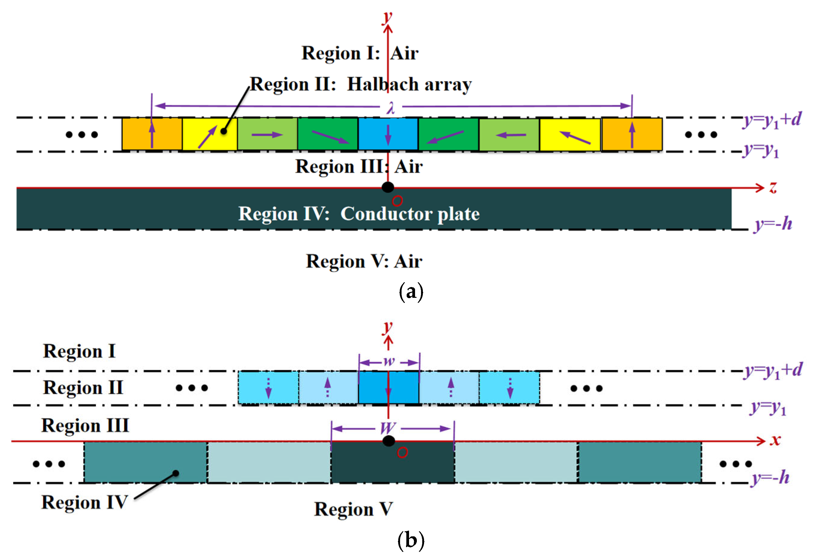
3. Three-Dimensional Electromagnetic Modelling

3.1. Magnetization Vector Expansion

When the Halbach array moves over a conductor plate in the z-direction, as shown in Figure 1, The original system can be extended by x-direction and z-direction if the edge effects are omitted. Suppose the PM reversible permeability is assumed equal to vacuum permeability. Thus, the distribution of magnetic field is periodic, and the y-axis component My of the magnetization vector can be expressed by
M y x ,   z , t = Re r = 1 + 4 B r M r μ 0 π 2 sin r π 2 sin r π 2 w W sin π M sin r π x W e j 2 π λ z 2 π v λ t
where Br is the remanence of the NdFeB magnet, μ0 is the permeability of the vacuum, λ is the wavelength of the Halbach array, M is the number of magnets in one period of the Halbach array, and v is the moving speed along the z-direction. Similiarly, the z-axis component Mz of the magnetization vector can be expressed by
M z x , z , t = Re r = 1 + j 4 B r M r μ 0 π 2 sin r π 2 sin r π 2 w W sin π M sin r π x W e j 2 π λ z 2 π v λ t

3.2. Governing Equations in Each Region

The whole space can be divided into five regions, as shown in Figure 1. Regions I, II, III, and V contain no free currents, and the scalar magnetic potential in each region is expressed by
φ i ( x , y , z , t ) = Re φ ˙ i ( x , y ) e j ( 2 π λ z 2 π v λ t ) ;   i = I ,   II ,   III ,   V
Region IV contains induced eddy currents, and can be describe by vector magnetic potential as
A n IV ( x , y , z , t ) = Re A ˙ n IV ( x , y ) e j ( 2 π λ z 2 π v λ t ) ;   n = x ,   y ,   z
Denote μ and σ, respectively, as the aluminum permeability (equal to vacuum permeability) and electrical conductivity. The X-axis component Mx of the magnetization vector is zero. Then, governing equations in each region are
2 A n IV ( x , y , z , t ) x 2 + 2 A n IV ( x , y , z , t ) y 2 + 2 A n IV ( x , y , z , t ) z 2 = μ σ A n IV ( x , y , z , t ) t ;   n = x ,   y ,   z  
2 φ i ( x , y , z , t ) x 2 + 2 φ i ( x , y , z , t ) y 2 + 2 φ i ( x , y , z , t ) z 2 = 0 ;   i = I ,   III ,   V · M x , M y , M z = M z x ,   z z ;   i = II

3.3. General Solutions to Governing Equations

Substituting Equation (3) into Equation (6) results in
2 φ ˙ i ( x , y ) x 2 + 2 φ ˙ i ( x , y ) y 2 2 π λ 2 φ ˙ i ( x , y ) = 0 ;   i = I ,   III ,   V   Re r = 1 + 8 B r M r μ 0 π λ sin r π 2 sin r π 2 w W sin π M sin r π x W e j 2 π λ z 2 π v λ t ;   i = II .    
For x = 0 and x = W, the scalar magnetic potentials were equal in the regions I, II, III, and V due to periodicity, and can be set to be zero. That is,
φ ˙ i ( 0 , y ) = φ ˙ i ( W , y ) = 0
Then, by the separation of the variables method, the solution to Equation (7) has a form of
φ ˙ i ( x , y ) = r = 1 + g ( y ) sin r π x W
Substitute Equation (9) into Equation (7), and it can be obtained that
g ( y ) = C 1 i e τ r y + C 2 i e τ r y ;   i = I ,   III ,   V C 1 i e τ r y + C 2 i e τ r y 8 B r M sin r π 2 sin r π 2 w W sin π M r μ 0 τ r 2 π λ ;   i = II
where, C 1 i and C 2 i are undetermined coefficients; τr has an expression of
τ r = 2 π λ 2 + r π W 2
Substitute Equation (4) into Equation (5), it holds that
2 A ˙ n IV ( x , y ) x 2 + 2 A ˙ n IV ( x , y ) y 2 = 2 π λ 2 2 j μ σ π v λ A ˙ n IV ( x , y ) ;   n = x ,   y ,   z
For x = 0 and x = W, the x-component of the induced eddy current is zero, and thus
A ˙ x IV ( 0 , y ) = A ˙ x IV ( W , y ) = 0 .
As a result of symmetry and periodicity, it holds that
A ˙ y IV ( x , y ) = A ˙ y IV ( x W , y ) = A ˙ y IV ( W x , y ) .
Let x = W/2, and it can be obtained that
A ˙ y IV ( W 2 , y ) = A ˙ x IV ( W 2 , y ) = 0 .
Similarly,
A ˙ z IV ( W 2 , y ) = A ˙ z IV ( W 2 , y ) = 0 .
Thus, the separation of variables method can be used to acquire the general solution to Equation (12)
A ˙ x IV ( x , y ) = r = 1 + D 1 r e α r y + D 2 r e α r y sin r π W x
A ˙ y IV ( x , y ) = r = 1 + E 1 r e α r y + E 2 r e α r y sin r π W x r π 2
A ˙ z IV ( x , y ) = r = 1 + F 1 r e α r y + F 2 r e α r y sin r π W x r π 2
where D 1 r , D 2 r , E 1 r , E 2 r , F 1 r , F 2 r are undetermined coefficients and
α r = a r + b r j = τ r 2 + τ r 4 + 4 μ 2 σ 2 π 2 v 2 / λ 2 2 2 j π μ σ v / λ 2 τ r 2 + τ r 4 + 4 μ 2 σ 2 π 2 v 2 / λ 2 .

3.4. Boundary Conditions

In the air, the magnetic field intensity is zero at infinity, so that the scalar magnetic potential is zero; no free currents exist at the boundary between the Halbach array and air, so that the magnetic field intensity and magnetic induction intensity are continuous. Free currents are considered to flow inside the conductor plate, and outer surface currents do not exist. Thus, the magnetic field intensity and magnetic induction intensity are also continuous at the boundary between the air and the conductor plate. Therefore, boundary conditions for the whole region can be expressed by
φ I ( x , + , z , t ) = 0
φ I ( x , y 1 + d , z , t ) y = φ I I ( x , y 1 + d , z , t ) y + M y
φ I ( x , y 1 + d , z , t ) z = φ I I ( x , y 1 + d , z , t ) z
φ II ( x , y 1 , z , t ) y + M y = φ III ( x , y 1 , z , t ) y
φ II ( x , y 1 , z , t ) z = φ III ( x , y 1 , z , t ) z
μ 0 φ III ( x , 0 , z , t ) x = A z IV ( x , 0 , z , t ) y A y IV ( x , 0 , z , t ) z
μ 0 φ III ( x , 0 , z , t ) y = A x IV ( x , 0 , z , t ) z A z IV ( x , 0 , z , t ) x
A z IV ( x , h , z , t ) y A y IV ( x , h , z , t ) z = μ 0 φ V ( x , h , z , t ) x
A x IV ( x , h , z , t ) z A z IV ( x , h , z , t ) x = μ 0 φ V ( x , h , z , t ) y
φ V ( x , , z , t ) = 0
Moreover, on the upper and lower surfaces of the conductor plate, the normal component of the eddy current is zero. Thus,
A ˙ y IV x , 0 = A ˙ y IV x , h = 0 .
Applying a Coulomb gauge on the vector magnetic potential, it holds that
A IV ( x , y 1 , z , t ) = A x IV x + A y IV y + A z IV z = 0 ;   i = IV  

3.5. Analytic Formulas of Electromagnetic Forces

The electric field distribution in the conductor plate can be expressed by
E x IV ( x , y , z , t ) = d A x IV ( x , y , z , t ) d t
E y IV ( x , y , z , t ) = d A y IV ( x , y , z , t ) d t
E z IV ( x , y , z , t ) = d A z IV ( x , y , z , t ) d t
The magnetic induction intensity components in the conductor plate are
B x IV ( x , y , z , t ) = A z IV ( x , y , z , t ) y A y IV ( x , y , z , t ) z
B y IV ( x , y , z , t ) = A x IV ( x , y , z , t ) z A z IV ( x , y , z , t ) x
B z IV ( x , y , z , t ) = A y IV ( x , y , z , t ) x A x IV ( x , y , z , t ) y
According to the above formulas, the lift force can be evaluated and approximated for high-speed conditions by
F L = l T 0 T h 0 0 W σ E z IV ( x , y , z , t ) B x IV ( x , y , z , t ) E x IV ( x , y , z , t ) B z IV ( x , y , z , t ) d x d y d t 2 l W B r 2 sin 2 π 2 w W M 2 sin 2 π M 1 + 2 π / λ 2 π λ 2 + π W 2 2 1 e 2 π λ 2 + π W 2 d 2 μ π 4 1 e 2 2 π λ 2 + π W 2 + 2 π λ 2 + π W 2 2 + μ 2 σ 2 v 2 2 π λ 2 2 h e 2 2 π λ 2 + π W 2 y 1
Similarly, the drag force can be calculated by
F D = l T 0 T h 0 0 W σ E x VI ( x , y , z , t ) B y VI ( x , y , z , t ) d x d y d t 4 l W π λ B r 2 M 2 sin 2 π M sin 2 π 2 w W 1 + 2 π / λ 2 π λ 2 + π W 2 2 π 4 μ 3 / 2 σ 1 / 2 v 1 / 2 1 e 2 π λ 2 + π W 2 d 2 1 e 2 2 π λ 2 + π W 2 + 2 π λ 2 + π W 2 2 + μ 2 σ 2 v 2 2 π λ 2 2 h e 2 2 π λ 2 + π W 2 y 1

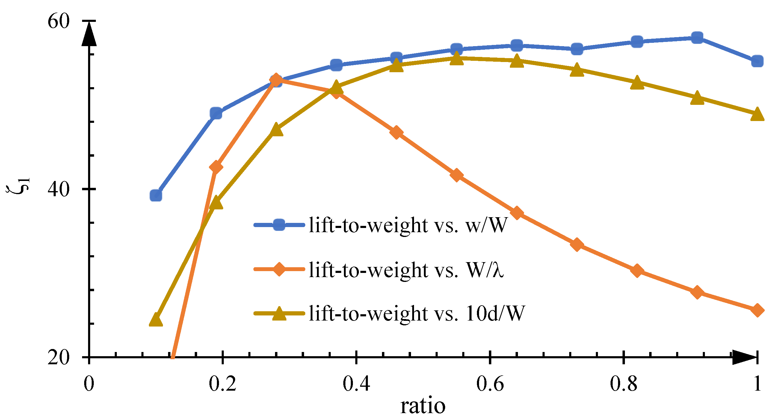
4. Structural Optimization

Lift-to-weight ratio and lift-to-drag ratio are two important indices to evaluate the PM EDS performance. Lift-to-weight ratio optimization is beneficial to improve the utilization of permanent magnets, and its is expressed by
γ = F L ρ g w l d = 2 W B r 2 sin 2 π 2 w W M 2 sin 2 π M 1 + 2 π / λ 2 π λ 2 + π W 2 2 1 e 2 π λ 2 + π W 2 d 2 μ π 4 ρ g w d 1 e 2 2 π λ 2 + π W 2 + 2 π λ 2 + π W 2 2 + μ 2 σ 2 v 2 2 π λ 2 2 h e 2 2 π λ 2 + π W 2 y 1
The ratios of w/W, W/λ, and d/W are three main independent parameters that make the lift-to-drag ratio non-monotonic varied. Parameters M, Br, W, y1, v, and h were set to 4, 1.28 T, 0.5 m, 15 mm, 300 m/s and 20 mm. It can be observed from Figure 2 that lift-to-drag ratio went up with the increase in the three ratios w/W, W/λ, and 10 d/W (note: we scaled d/W by a factor of 10 to ensure its range fell between 0 and 1), and then decreased in general; the max values of lift-to-drag ratio were different, indicating the three ratios should be simultaneously optimized.
The lift-to-drag ratio characterizes the energy consumption and can be evaluated by
ζ = F L F D = 1 2 μ v λ π
The lift-to-drag ratio was linear with the square root of the product of wavelength and moving speed, while the lift-to-weight ratio was nonlinear with each structural parameter. Thus, the lift-to-weight ratio was chosen as the optimization index. We rewrote the lift-to-weight ratio as
γ = 2 B r 2 1 e 2 2 π λ 2 + π W 2 + 2 π λ 2 + π W 2 2 + μ 2 σ 2 v 2 2 π λ 2 2 h μ π 2 ρ g M 2 π 2 sin 2 π M W sin 2 π 2 w W w 1 e 2 π λ 2 + π W 2 d 2 2 π λ 2 + π W 2 d 2 π λ 2 + π W 2 1 + 2 π / λ 2 π λ 2 + π W 2 2 e 2 2 π λ 2 + π W 2 y 1 = 2 B r 2 μ π 2 ρ g M 2 π 2 sin 2 π M 1 β 1 sin 2 π 2 β 1 1 e π β 3 4 β 2 2 + 1 2 π β 3 4 β 2 2 + 1 π W 4 β 2 2 + 1 1 + 2 β 2 4 β 2 2 + 1 2 e 2 π β 4 4 β 2 2 + 1
where β 1 = w W , β 2 = W λ , β 3 = d W , β 4 = y 1 W . The second term on the right side of Equation (43) increased as M became large and varied little when M ≥ 8, as shown in Table 1. Thus, the larger M is, the better.
Taking the width of the conductor plate W as a parameter and w as a variable, let
f = 1 β 1 sin 2 π 2 β 1 β 3 = sin π β 1 2 π β 1 cos π β 1 2 sin π 2 β 1 β 3 2 = sin π β 1 2 cos π β 1 2 π β 1 tan π 2 β 1 β 1 2
When 0 < β1 < 0.742, f > 0 , while when 0.742 < β1 < 1, f < 0 . Thus, when β1 = 0.742, 1 β 1 sin 2 π 2 β 1 reaches the maximum.
Similarly, 1 e π β 3 4 β 2 2 + 1 2 π β 3 4 β 2 2 + 1 reaches the maximum when β 3 4 β 2 2 + 1 = 0.4 ; W and β4, taken as parameters, when 2 π β 2 β 4 + β 2 4 β 2 2 + 1 = 1 , π W 4 β 2 2 + 1 1 + 2 β 2 4 β 2 2 + 1 2 e 2 π β 4 4 β 2 2 + 1 reaches the maximum. To sum up, given the width of the conductor plate W and levitation gap y1 (that is, β4 given), the lift-to-weight ratio reaches the maximum if and only if
β 1 = 0.742 β 3 4 β 2 2 + 1 = 0.4 2 π β 2 β 4 + β 2 4 β 2 2 + 1 = 1
When W→∞, Equation (45) degrades into the 2D optimization result shown in the literature [22] as
2 π λ d = 1.2564 λ = 4 π y 1

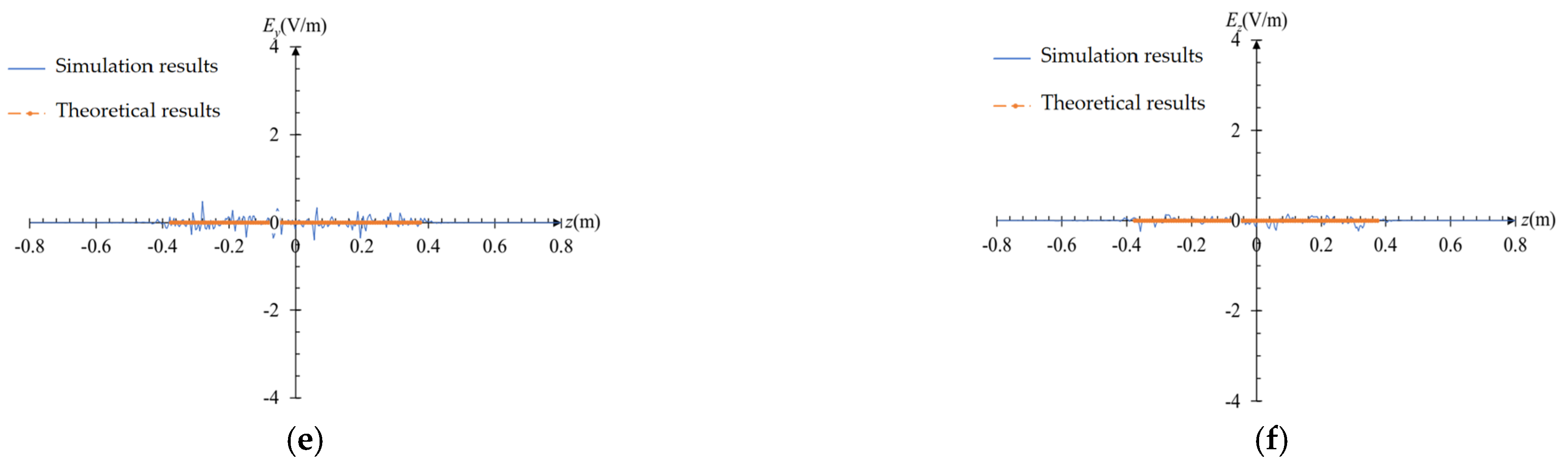
5. Simulation Verification

A total of three wavelengths of Halbach permanent magnet arrays were selected, with an angular difference of π/4 between adjacent permanent magnets. The material of the permanent magnets was N52, with a remanence of 1.44 T. The magnetization angles of the permanent magnets were sequentially 3π/2, π, π/2, π/4, 0, …, 3π/2. To form a complete magnetic circuit and minimize the impact of end effects, 25 permanent magnets were chosen for the simulation, ensuring that the magnetization angles of the two end magnets were identical. The arrows indicate the magnetization direction of the permanent magnet array. The wavelength of the permanent magnet array was set to 240 mm, with a height of 30 mm. The thickness of the aluminum plate was 30 mm, and the gap between it and the permanent magnet array was 15 mm. The width of the permanent magnet array was 60 mm, and the width of the conductor plate was 100 mm. A steady-state model was used for the solution. The coordinate system was set as shown in Figure 3, with the projection of the geometric center of the permanent magnet array on the upper surface of the conductor plate at (0.05, 0, 0). The z-axis pointed to the right, the y-axis direction was vertically upward, and the x-axis pointed into the paper. A target line was selected that passed through the coordinate point (0.05, −0.001, 0) and was parallel to the z-axis. The distribution of magnetic flux density and eddy current field strength along the target line was investigated. A velocity of 300 m/s towards the horizontal direction was applied to the conductor plate.
The FEM simulation used a mesh with 2,104,086 tetrahedral elements. The estimated energy error for the simulation was 0.5%. The distribution of the magnetic flux density (in the x, y, and z directions) along the target line is shown in Figure 4. Overall, the peak values of the normal component Bx and the vertical component By were significantly smaller than that of the horizontal component Bz, and both were approximately one order of magnitude lower in magnitude. On the target line, the peak value of the normal component Bx was around 0.02 T, the peak of the vertical component By was 0.04 T, and the peak of the horizontal component Bz was approximately 0.4 T. This indicates that the horizontal component of the magnetic flux density dominated. In the non-end regions, the magnetic field exhibited a periodic distribution with a wavelength of 0.24 m, which is consistent with the theoretical assumption of the fundamental wavelength of the electromagnetic field, demonstrating the rationality of the theoretical assumption. On the target line, the theoretical electromagnetic field curve aligned well with the finite element simulation curve, proving the accuracy of the 3D theoretical electromagnetic field model.

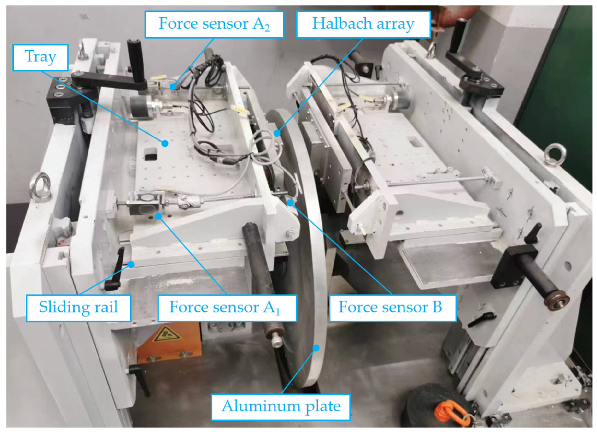
6. Experimental Verification

To verify the correctness of Equation (39) and Equation (40), a platform (equipped with the PM Halbach array and a rotary aluminum plate with flange was used to simulate the linear motion of the designed rocket sled above a finite wide rail. As shown in Figure 5, the flange at the edge of the plate was designed for simulating the finite wide rail. The total number and magnetized direction of the magnets was the same as the former simulation, except that the material of the magnets was N52. Note that the mechanism on the right side of the plate persevered for another purpose and did not participate in the experiment. The Halbach array adopted the optimized size in the former simulation. The aluminum plate had a thickness of 30 mm and radius of 0.4 m. Its flange had a thickness of 10 mm and a width of 90 mm. The length of the Halbach array was so small compared with the perimeter of the plate that the motion can be regarded as a linear motion. An electric motor drove the plate moving at a linear speed of 0~52 m/s. The sliding bearing enabled the Halbach array to be free along the tangential direction at the edge of the plate, ensuring force sensor B captured the drag force. The sliding rails on both sides allowed the Halbach array to move freely along the axial direction of the plate. Thus, force sensors A1 and A2 can be used to measure the lift force. The center line of the Halbach array was aligned with that of the flange.
The force transducers used in the experiments were SK-LK01, with an accuracy of ±0.05% of the full-scale range. Electromagnetic force comparison between the 3D analytics and 3D simulation is shown in Figure 6. The 3D analytic lift force increased sharply as the speed went up initially, and then it became steady when the speed was beyond 10 m/s. The 3D analytical lift force coincided well with the 3D simulated one with an error less than 12%. Yet, in the former research [22], the 2D analytical lift force had an error of more than 50% with the 3D simulated one. The 3D analytical lift force deviated less than 26% with the experimental one. The deviation was also much smaller than the 2D case (beyond 70%) in the former research [22]. Thus, the 3D model led to a much smaller error than the 2D model in the former research.
Drag forces obtained by the 3D analytical, simulated, and experimental methods were highly consistent. The error between the 3D analytical drag force and the 3D simulated one was within 5%. Conversely, in the former research [22], the error was about 50% in the 2D case. The difference between the 3D analytical drag force and the experimental one was within 16%. Similarly, the difference was also smaller than the 2D case (beyond 60%) in the former research [22].
The difference between the 3D analytical forces and measured forces was obvious. On one hand, this was because the three-dimensional theoretical model neglected the influence of longitudinal and transverse end effects on the calculation of electromagnetic forces. On the other hand, the eddy currents in the rotating disk were not entirely concentrated beneath the permanent magnet array; instead, a portion diffused radially toward the center of the disk, which differed from the symmetric distribution of eddy currents in the actual linear track. Additionally, temperature rise led to a decrease in the electrical conductivity of the disk, resulting in a reduction in eddy current intensity and, consequently, a decrease in electromagnetic forces.
To sum up, Equations (39) and (40) were correct in showing that the 3D modeling method proposed in the paper was valid. The 3D modeling method had an advantage over the 2D one, greatly reducing the errors of the electromagnetic force formulas.

7. Conclusions

In this paper, analytical 3D mathematical modelling was conducted for a PM Halbach array moving over a conductor plate designed for the ultra-high-speed rocket sled. A periodically extended method was proposed to provide the brief formulas of the electromagnetic forces, including lift force and drag force. Lift-to-weight and lift-to-drag ratios revealed an inherent link between the 3D and 2D models. The 3D electromagnetic force model was validated by simulation and experiments, showing higher accuracy than the 2D model in earlier study.

Author Contributions

Writing—original draft, Y.H. and B.C.; Writing—review & editing, G.L. and Z.W. All authors have read and agreed to the published version of the manuscript.

Funding

This work was supported by the National Natural Science Foundation of China (Key Program), grant numbers: 52432012, 52332011.

Data Availability Statement

Data are contained within the article.

Conflicts of Interest

The authors declare no conflicts of interest.

References

  1. Long, Z.Q.; Li, X.L.; Cheng, H. Research on Permanent-Electromagnetic Levitation Technology and Application; Shanghai Scientific and Technical Publishers: Shanghai, China, 2019. [Google Scholar]
  2. Cinnamon, J.D.; Palazotto, A.N.; Szmerekovsky, A.G. Further Refinement of Material Models for Hypervelocity Gouging Impacts. AIAA J. 2018, 46, 317–327. [Google Scholar] [CrossRef]
  3. Hooser, M. 6 DoF Model of the Holloman High Speed Test Track Maglev Sled. In Proceedings of the US Air Force T&E Days, Nashville, Tennessee, 2–4 February 2010; p. 1706. [Google Scholar]
  4. Minto, D. Recent increases in hypersonic test capabilities at the Holloman High Speed Test Track. In Proceedings of the 38th Aerospace Sciences Meeting and Exhibit, Reno, NV, USA, 10–13 January 2000; p. 154. [Google Scholar]
  5. Hsu, Y.; Langhorn, A.; Ketchen, D.; Holland, L.; Minto, D.; Doll, D. Magnetic levitation upgrade to the Holloman high speed test track. IEEE Trans. Appl. Supercond. 2009, 19, 2074–2077. [Google Scholar] [CrossRef]
  6. Gurol, H.; Ketchen, D.; Holland, L.; Minto, D.; Hooser, M.; Bosmajian, N. Status of the Holloman high speed MagLev test track (HHSMTT). In Proceedings of the 30th AIAA Aerodynamic Measurement Technology and Ground Testing Conference, Atlanta, GA, USA, 16–20 June 2014; p. 2655. [Google Scholar]
  7. Xuesong, Q.; Qianyuan, S.; Zikang, S.; Yuhang, L.; Bin, W. Analysis of the magnetic levitation characteristics of the vertical Halbach array in a permanent magnet rotor. Nonlinear Dyn. 2025, 113, 397–412. [Google Scholar] [CrossRef]
  8. Li, Q.; Ma, C.; Gao, F. Nonlinear model for Halbach array axial flux permanent magnet motor in stator and rotor reference frames based on harmonic modeling technique. IEEE Trans. Magn. 2024, 60, 8201811. [Google Scholar] [CrossRef]
  9. Vatani, M.; Chulaee, Y.; Mohammadi, A.; Stewart, D.R.; Eastham, J.F.; Ionel, D.M. On the optimal design of coreless AFPM machines with Halbach array rotors for electric aircraft propulsion. In Proceedings of the 2024 IEEE Transportation Electrification Conference and Expo (ITEC), Chicago, IL, USA, 19–21 June 2024; pp. 1–6. [Google Scholar]
  10. Hu, Y.P.; Long, Z.Q.; Xu, Y.S.; Wang, Z.Q. Control-oriented modeling for the electrodynamic levitation with permanent magnet Halbach array. Int. J. Appl. Electromagn. Mech. 2021, 67, 375–3921. [Google Scholar] [CrossRef]
  11. Shi, H.; Deng, Z.; Ke, Z.; Li, Z.; Zhang, W. Linear permanent magnet electrodynamic suspension system: Dynamic characteristics, magnetic-mechanical coupling and field test. Measurement 2024, 225, 113960. [Google Scholar] [CrossRef]
  12. Shi, H.; Ke, Z.; Zheng, J.; Xiang, Y.; Ren, K.; Lin, P.; Li, K.; Liang, L.; Deng, Z. An effective optimization method and implementation of permanent magnet electrodynamic wheel for Maglev car. IEEE Trans. Veh. Technol. 2023, 72, 8369–8381. [Google Scholar] [CrossRef]
  13. Sun, H.; Cheng, S.S. A cylindrical Halbach array magnetic actuation system for longitudinal robot actuation across 2D workplane. IEEE Robot. Autom. Lett. 2024, 9, 5847–5854. [Google Scholar] [CrossRef]
  14. Shi, H.; Wu, S.; Ke, Z.; Deng, Z.; Zhang, W. Speed-Range-Based Novel Guideway Configuration with Variable Material and Thickness for PMECB. IEEE Trans. Instrum. Meas. 2024, 73, 2514913. [Google Scholar] [CrossRef]
  15. Hirde, A.; Khardenavis, A.; Banerjee, R.; Bose, M.; Hari, V.S.P.K. Energy and emissions analysis of the hyperloop transportation system. Environ. Dev. Sustain. 2023, 25, 8165–8196. [Google Scholar] [CrossRef]
  16. Wang, B.; Luo, S.; Ma, W.; Li, G.; Wang, Z.; Xu, J.; Zhang, X. A fast dynamic model of a two-sided permanent magnet electrodynamic suspension system in a maglev train. Proc. Inst. Mech. Eng. Part F J. Rail Rapid Transit 2023, 237, 996–1008. [Google Scholar] [CrossRef]
  17. Luo, C.; Zhang, K.; Zhang, H. Effect of the passive damping plate on the vertical stability of permanent magnet electrodynamic suspension system. IET Electr. Power Appl. 2024, 18, 107–115. [Google Scholar] [CrossRef]
  18. Flankl, M.; Wellerdieck, T.; Tüysüz, A.; Kolar, J.W. Scaling laws for electrodynamic suspension in high-speed transportation. IET Electr. Power Appl. 2018, 12, 357–364. [Google Scholar] [CrossRef]
  19. Qin, W.; Ma, Y.; Lv, G.; Wang, F.; Zhao, J. New Levitation Scheme with Traveling Magnetic Electromagnetic Halbach Array for EDS Maglev System. IEEE Transactions on Magnetics 2022, 58, 8300106. [Google Scholar] [CrossRef]
  20. Liu, J.; Cao, T.; Deng, Z.; Shi, H.; Liang, L.; Wu, X.; Jiang, S. Damping characteristics improvement of permanent magnet electrodynamic suspension by utilizing the end-effect of onboard magnets. Electr. Eng. 2024, 106, 15–29. [Google Scholar] [CrossRef]
  21. Long, Z.Q.; He, G.; Xue, S. Study of EDS & EMS Hybrid Suspension System with Permanent-Magnet Halbach Array. IEEE Trans. Magn. 2011, 47, 4717–4724. [Google Scholar]
  22. Hu, Y.P.; Long, Z.Q.; Zeng, J.; Wang, Z.Q. Analytical Optimization of Electrodynamic Suspension for Ultrahigh-Speed Ground Transportation. IEEE Trans. Magn. 2021, 57, 8000511. [Google Scholar] [CrossRef]
Figure 1. Extension of the Halbach array–conductor plate system and whole region division. (a) Extension along the z-axis. (b) Extension along the x-axis. The arrow means the magnetization direction of each permanent magnet.
Actuators 14 00225 g001
Figure 2. Lift-to-weight ratio variation with w/W, W/λ, and d/W.
Actuators 14 00225 g002
Figure 3. The three-dimensional FEM geometric model.
Actuators 14 00225 g003
Figure 4. Comparison between numerical simulation and analytical calculation results for the PM Halbach array moving over the aluminum conductor plate. (a) Bx distribution. (b) By distribution. (c) Bz distribution. (d) Ex distribution. (e) Ey distribution. (f) Ez distribution.
Actuators 14 00225 g004aActuators 14 00225 g004b
Figure 5. Rotary device built for testing electromagnetic forces when the Halbach array “moved” over a conductor plate. Force sensors A1 and A2 were used to capture the lift force, while force sensor B captured the drag force.
Actuators 14 00225 g005
Figure 6. Electromagnetic forces comparison of the 3D analytical electromagnetic forces with both the 3D simulated and experimental results.
Actuators 14 00225 g006
Table 1. Values for M adopting different values.
M24681012
M 2 π 2 sin 2 π M 0.410.810.910.950.970.98
Disclaimer/Publisher’s Note: The statements, opinions and data contained in all publications are solely those of the individual author(s) and contributor(s) and not of MDPI and/or the editor(s). MDPI and/or the editor(s) disclaim responsibility for any injury to people or property resulting from any ideas, methods, instructions or products referred to in the content.

