Optimization of Unmanned Excavator Operation Trajectory Based on Improved Particle Swarm Optimization

Abstract

To realize the autonomous operation of unmanned excavators, this study takes the four-axis manipulator arm of an unmanned excavator as the research object, uses the five-order B-spline curve for operation trajectory planning, and proposes an improved particle swarm optimization algorithm for the continuous trajectory optimization problem of excavator single operation. The specific contents are as follows: based on the standard PSO algorithm, dynamic parameter update is used to enhance the global search ability in the early stage and improve the local search accuracy in the later stage; the diversity monitoring mechanism is enhanced to avoid premature maturity convergence; multi-particle SA perturbation is introduced, and the new solution is accepted according to the Metropolis criterion to enhance global search ability. The adaptive cooling rate flexibly responds to different search situations and improves the search efficiency and quality of the solution. To verify the effectiveness of the improved PSO–SA algorithm, this study compares it with the standard PSO algorithm, the standard PSO–SA algorithm, and the MPSO algorithm. The simulation results show that the improved PSO–SA algorithm can converge to the global optimal solution more quickly, has the shortest time in trajectory planning, and the generated trajectory has higher tracking accuracy, which ensures that the vibration and impact of the manipulator during motion are effectively suppressed.

1. Introduction

At present, the accelerated development of artificial intelligence technology, the Internet of Things, and big data have injected a strong impetus concerning the intelligence of construction machinery. However, the traditional excavator operation mode has exposed many drawbacks: on the one hand, it is difficult to improve the efficiency of manual operation, which seriously restricts the progress of the project; on the other hand, operations in hazardous environments lead to frequent casualties, which pose a huge threat to personnel safety. In this context, unmanned and precise operation is realized through trajectory planning, which provides an effective way to solve the pain points of traditional excavator operations. From the perspective of construction efficiency, unmanned precision operation overcomes the limitations of human beings, achieves efficient and stable construction operations, and significantly improves construction speed and quality [1]. From the perspective of personnel safety, this can keep operators away from hazards, effectively reduce the risk of casualties, and has significant safety advantages. In addition, unmanned and precise operation [2] can also break through the limitation of continuous operation time, realize all-weather uninterrupted construction, and further improve the utilization rate and economic benefits of construction machinery. Therefore, trajectory planning is the key to optimizing the joint movement parameters in order to achieve a smooth transition and improve efficiency and longevity.

In the field of trajectory planning, the research results of polynomial trajectory programming and curve trajectory programming have laid the foundation for subsequent optimization. Liao et al. [3] proposed a PUMA560 robot trajectory planning method based on quintic polynomial interpolation, the accuracy and smoothness of the kinematic model are verified by using the Denavit–Hartenberg model and the simulation of the MATLAB robot toolbox, the continuity of joint motion is realized in the pick-and-place operation, and the peak angular velocity is less than 1.85 rad/s. Potter et al. [4] proposed an energy optimization framework for redundant planar manipulators based on quadratics. Compared with the traditional cubic spline method, the energy consumption of the 7DOF system is reduced by 24.8%, and the calculation time is controlled within 2.1 s. In addition, Sun et al. [5] construct a multi-objective trajectory planning framework for shield segment assembly robots based on B-spline interpolation and non-feasible solution update with improved non-dominated ordering, and its Pareto optimization model simultaneously improves time efficiency, acceleration continuity, and mechanical shock suppression. In Liu et al. [6], the enhanced Bottle Squirt Swarm Algorithm (LMSSA) was combined with the artificial potential field method, and the energy consumption and vibration amplitude were reduced by 18.9% and 42.3% compared with the genetic algorithm method through seventh-order B-spline parameterization and LMSSA node optimization.

On this basis, the research on multi-objective trajectory optimization algorithms further promotes the development of trajectory planning. Bi [7] In the first stage, the mining time and energy consumption per unit load are minimized under the constraints of kinematics and geometry, and operation feasibility is enhanced by optimizing the speed curve of the actuator in the second stage. The application of the method on the WK-55 excavator shows that the proposed method improves energy efficiency by 13.28% through trajectory smoothing and achieves computational convergence within 150 iterations. In Zhang et al. [8], the proposed improved Ant Colony Optimization (ACO) algorithm optimizes the algorithm by adaptive grid division, improved pheromone update mechanism and extended ant visual perception range, and the experimental results show that the improved ACO shortens the path search time by 37.6% compared with the traditional method, while maintaining obstacle avoidance ability and improving path smoothness. In Wu et al. [9], the proposed improved TSO algorithm is used for the time-optimal trajectory planning of the 6-degree-of-freedom manipulator, and the convergence probability is increased by 89.7% compared with the standard TSO. The 3-5-3 hybrid polynomial implementation reduces trajectory duration by 22.4% while maintaining velocity continuity and acceleration boundaries. Xidias [10] proposed a time-optimal trajectory planning method for super-redundant robotic arms in three-dimensional workspaces. This method uses the Hyper-BumpSurface concept to represent the three-dimensional workspace, unifying free space and obstacle space into a single mathematical entity, which reduces the computational complexity and storage requirements of traditional configuration space (C-space) methods. By transforming the time-optimal trajectory planning problem into a global optimization problem and solving it using a multi-agent genetic algorithm (MPGA), this study verified the effectiveness of the proposed method through various simulation experiments. Zacharia and Xidias [11] investigated the task scheduling optimization problem for robots in complex environments, taking mechanical advantage into account. The paper aims to maximize mechanical advantage, considering three optimization criteria: cycle time, collision avoidance, and the mechanical advantage index, and achieves optimization by combining genetic algorithms with the Bump–Surface concept. In summary, the research on polynomial trajectory planning and curve trajectory planning provides a basic method for the trajectory planning of the robotic arm, while the multi-objective trajectory optimization algorithm realizes the optimization of time, energy consumption, smoothness, and other aspects through different intelligent optimization methods.

In this study, the improved PSO–SA algorithm was used to optimize the spatial trajectory of the joint of the excavator manipulator to realize the unmanned excavation operation. The specific research contents of this study are as follows:

(1)

Taking a certain type of unmanned excavator manipulator in the laboratory as the research object, to achieve optimal performance of the joint space trajectory planning for the unmanned excavator manipulator, the three parameters of time, smoothness and energy were comprehensively compared with the cubic polynomial, the fifth polynomial, the B-spline curve, and the three trajectory planning methods, and finally the B-spline curve was selected to complete the joint space operation trajectory planning, and the excavation bucket was carried out from the starting point to the target point in a controllable manner.

(2)

To further improve the operation efficiency of the unmanned excavator, the improved PSO–SA algorithm was used to optimize the operation trajectory of the B-spline curve with minimum time and energy as the optimization goals, and the MATLAB robot toolbox was used to simulate and test this, and PSO, standard PSO–SA, and improved PSO–SA and MPSO were used to optimize the operation trajectory of B-spline curve planning. The trajectory planning results for the four algorithms were compared and analyzed, and the trajectory with the lowest time and energy consumption and the most stable algorithm strategy was obtained.

2. Materials and Methods

2.1. Kinematic Analysis of Unmanned Excavator Operation

2.1.1. Introduction to a Certain Type of Unmanned Excavator

Taking a certain model of unmanned excavator robotic arm in the laboratory as the research object, its structural diagram is shown in Figure 1. The unmanned excavator manipulator arm is a key part of the excavation and loading operations, and its structural design and performance will directly affect the operation efficiency. The device is mainly composed of a boom mechanism, a stick mechanism, a bucket assembly, a turntable, a drive system, and a linkage mechanism. Through the precise coordination of each component, four degrees of freedom can be realized: the boom swings up and down, the stick expands and expands backwards and forwards, the bucket moves in a complex manner, and the turntable rotates.

2.1.2. Kinematic Analysis of the Excavator Manipulator Arm

The accuracy of the kinematic formula directly affects the feasibility and effectiveness of trajectory planning, so the accuracy of the model should be ensured in practical applications. By combining the motion parameters of the individual joints, a complete kinematic model is built to describe the motion relationship of each part from the base to the bucket. The Denavit–Hartenberg (DH) parameter method is commonly used [12] to systematically describe the position and posture of each joint.

As shown in Figure 2, a fixed coordinate system is established on each joint connecting rod. The coordinate system relationship between the two adjacent rods is described by using the homogeneous transformation matrix, and the posture of each segment of the robotic arm is represented as the relationship between different homogeneous matrices. Knowing the technical parameters and D–H coordinate system of the manipulator, the D–H parameter table and the parameters of each joint of the manipulator are shown in

Table 1. D–H parameters of unmanned excavator manipulator.

Joint i	${\mathit{a}}_{\mathit{i}-1}$	${\mathit{\alpha }}_{\mathit{i}-1}$	${\mathit{d}}_{\mathit{i}}$	${\mathit{\theta }}_{\mathit{i}}$
1	$a_0$	${\displaystyle \frac{\pi }{2}}$	$d_0$	${\theta }_1$
2	L1	0	0	${\theta }_2$
3	L2	0	0	${\theta }_3$
4	L3	0	0	${\theta }_4$

. The twist angle $\mathsf{\alpha }$ is the angle between the two adjacent Z-axes, the connecting rod length a is the minimum distance between the two adjacent Z-axes, the joint variable $\mathsf{\theta }$ is the angle between the two adjacent Z-axes, and the connecting rod offset d is the distance between the two common normals, and its magnitude is equal to the distance between the two X-axes [13].

${\mathit{a}}_{\mathit{i}-1}$$a_0$${\displaystyle \frac{\pi }{2}}$$d_0$${\theta }_1$${\theta }_2$${\theta }_3$${\theta }_4$ According to the above parameters, the homogeneous transformation matrix of each joint is calculated, and the total transformation matrix from the base coordinate system to the bucket coordinate system is obtained by multiplying as follows:

$${T_i}^{i-1}=\left[\begin{array}{cccc}\cos {\theta }_i& -\cos {\alpha }_i\sin {\theta }_i& \sin {\alpha }_i\sin {\theta }_i& a_i\cos {\theta }_i\\ \sin {\theta }_i& \cos {\alpha }_i\cos {\theta }_i& -\cos {\alpha }_i\sin {\alpha }_{i-1}& a_i\sin {\theta }_i\\ 0& \sin {\alpha }_i& \cos {\alpha }_i& d_i\\ 0& 0& 0& 1\end{array}\right]$$

(1)

$$T_4^0=T_1^0{T}_2^1{T}_3^2{T}_4^3$$

(2)

$$T_4^0=\left[\begin{array}{cccc}{c}_1{c}_{234}& -c_1{s}_{234}& s_1& c_1(L_3{c}_{234}+L_2{c}_{23}+L_1{c}_2+a_0)\\ s_1{s}_{234}& -s_1{s}_{234}& -c_1& s_1(L_3{s}_{234}+L_2{s}_{23}+L_1{c}_2+a_0)\\ s_{234}& c_{234}& 0& L_3{c}_{234}+L_2{s}_{23}+L_1{s}_2+d_0\\ 0& 0& 0& 1\end{array}\right]$$

(3)

where: $c_{23}=\cos ({\theta }_2+{\theta }_3)$, $c_{234}=\cos ({\theta }_2+{\theta }_3+{\theta }_4)$, $s_{23}=\sin ({\theta }_2+{\theta }_3)$, $s_{234}=\sin ({\theta }_2+{\theta }_3+{\theta }_4)$, $c_2=\cos {\theta }_2$, $s_1=\sin {\theta }_1$, $s_2=\sin {\theta }_2$.

L₁, boom length; L₂, stick length; L₃, bucket length; a₀, coordinate system 0 and coordinate system 1 in the x direction; d₀, coordinate system 0 and coordinate system 1 in the y direction.

According to Equation (3), the position of the bucket tip is expressed as a vector [X,Y,Z]^T, and its coordinates are:

$$x=\cos {\theta }_1(L_3\cos ({\theta }_2+{\theta }_3+{\theta }_4)+L_2\cos ({\theta }_2+{\theta }_3)+L_1\cos {\theta }_2+a_0)$$

(4)

$$y=\sin {\theta }_1(L_3\sin ({\theta }_2+{\theta }_3+{\theta }_4)+L_2\sin ({\theta }_2+{\theta }_3)+L_1\cos {\theta }_2+a_0)$$

(5)

$$z=L_3\cos ({\theta }_2+{\theta }_3+{\theta }_4)+L_2\cos ({\theta }_2+{\theta }_3)+L_1\cos {\theta }_2+d_0)$$

(6)

2.2. Improving the Trajectory Optimization of Particle Swarm Optimization

2.2.1. Trajectory Planning Methods

The joint space trajectory planning directly acts on the joint space of the robot, accurately plans the angle, angular velocity, and angular acceleration of each joint, and converts it into a function of time. This planning method maps the path requirements of the task space to the joint space through inverse kinematics and generates the corresponding motion parameters [14]. Joint space trajectory planning eliminates the need to frequently calculate Cartesian space paths in the real-time control process, which greatly simplifies the complex process of coordinate transformation and significantly improves the speed and efficiency of calculation. At the same time, there is no continuous mapping relationship between the joint space and the Cartesian space, which makes the robot avoid the singularity problem during movement [15].

Through cubic polynomials, fifth-order polynomials, B-spline curves, and other methods, joint space trajectory planning can be carried out. The cubic polynomial calculation is simple and real-time in nature, but the acceleration may change abruptly at the node, resulting in mechanical shock. The fifth-order polynomial has good high-order smoothness and continuous acceleration and reduces mechanical vibration and shock, but its calculation is complex and requires the solution of a six-element equation, and the amount of computation increases exponentially with the increase in the number of path points.The B-spline [16] can adjust individual control points to affect only a local trajectory, which is suitable for online optimization, and acceleration continuity can be achieved by selecting the node vector order. However, the basis function needs to be calculated recursively, and the real-time performance is limited.

This paper evaluates the trajectory performance of different methods using smoothness, energy consumption, and computation time. In the field of trajectory planning, smoothness is a key performance metric that measures the fluidity and continuity of the trajectory curve. This paper comprehensively assesses the overall smoothness of the trajectory by calculating the squared integral of acceleration over the trajectory. Energy consumption is an important indicator for evaluating the economic and efficiency aspects of trajectory planning methods; it reflects the total amount of energy consumed by the system during its movement along the planned trajectory. In mechanical systems, the energy required to overcome inertia is proportional to the square of the acceleration, so this paper uses this simplified model to evaluate the energy consumption required for trajectory planning. In order to realize the optimal trajectory planning of the unmanned excavator operation, the above three methods are used in MATLAB 2020 b to plan the trajectory between two points of the robotic arm. The spatial motion path of the robot arm is shown in Figure 3. and the simulation results are shown in Figure 4 below. From the perspective of the velocity and acceleration curve charts, the cubic polynomial curve fluctuates greatly in terms of velocity and acceleration, which may lead to large shocks and vibrations during the movement of the robotic arm. The fifth-order polynomial curve shows improvement in terms of smoothness, but there are still some fluctuations. The B-spline curve has the best performance in terms of robotic arm to achieve smoother and precise motion control, effectively reduce mechanical wear and energy consumption, and improve the stability and reliability of the system.

The performance parameters of the three methods are shown in

Table 2. Performance parameters of single operation trajectory planning method.

Evaluation Indicators	Cubic Polynomials	Fifth-Order Polynomials	B-Spline
Calculate time/s	0.0916	0.0935	0.1187
Smoothness	0.1501	0.7216	0.2812
energy consumption	0.3159	0.4512	0.1843

, and the normalized performance parameters are shown in

Table 3. The normalized evaluation results of performance parameters for trajectory planning method are obtained.

Evaluation Indicators	Cubic Polynomials	Fifth-Order Polynomials	B-Spline
Calculate the time	0	−0.070	−1.000
Smoothness	0	−1	−0.229
energy consumption	−0.493	−1	0
Overall score	−0.296	−0.814	−0.246
Overall ranking	2	3	1

. The cubic polynomial calculation time and smoothness score are 0, the energy consumption is negative, the comprehensive score is low, and the overall ranking is second. The scores of all indicators of the five polynomials are negative, and the comprehensive score is the lowest, ranking third overall. The energy consumption score of the B-spline curve is 0, the smoothness and computational time scores are negative, and the comprehensive score is the highest, ranking first overall, indicating that the computational efficiency is high and the comprehensive performance is good. The B-spline curve is used for the trajectory planning of the mining task by comprehensively analyzing the B-spline curve with the least time and energy consumption and the best smoothness in the trajectory planning of the manipulator arm.

2.2.2. B-Spline Trajectory Planning

B-spline [17,18,19]. The curve has a stable mathematical model, good local support performance, and excellent geometric properties, and has been widely used in trajectory planning. At the same time, as an extension of the Bezier curve, the B-spline curve realizes the flexible control of complex trajectories through the piecewise polynomial function. In this paper, the 5th order B-spline function is used for trajectory planning in the joint space of the excavator manipulator, and the main contents are as follows: the mathematical expression of k times B-spline curve can be defined as [20].

$$C(u)={\displaystyle \sum _{i=0}^n{N}_{i,k}(u)}{P}_i$$

(7)

where: $N_{i,k}\left(u\right)$ is the kth degree B spline basis function, $P_i$ is the control point.

The basic functions are generated by the Cox-de Boor recursive formula:

$$N_{i,0}(u)=\left\{\begin{array}{c}1\\ 0\end{array}\right.\begin{array}{c}{u}_i\le u<u_{i+1}\\ otherwises\end{array}$$

(8)

$$N_{i,k}(u)={\displaystyle \frac{u-u_i}{u_{i+k}-u_i}}{N}_{i,k-1}(u)+{\displaystyle \frac{u_{i+k+1}-u}{u_{i+k+1}-u_{i+1}}}{N}_{i+1.k-1}(u)$$

(9)

In this study, a continuous trajectory was planned for an excavation task and, for each trajectory, five B-spline curves were used for trajectory planning with known joint value points at the beginning and end. In order to make all the joints of the manipulator M pass through the given shape value points ^MQ_i, the control vertices of the joint trajectory of the B-spline curve need to be solved ^MD_j, and the first and last points of the curve must coincide with the beginning and end of the given shape value points. The node vector can be expressed as T = [t₀,t₁,$\cdots$t_{n + k + 1}] as follows: in order to ensure that the beginning and end values of the spline coincide with the beginning and end of the control curve, the beginning and end of the curve node should have a repeatability of k + 1, i.e., t₀ = t₁ = … = t_k = 0, t_{n + 1} = t_{n + 2} = … = t_{k + n + 1} = t_i.

According to the node vector T, the type-value point ^MQ_i and the basis function N_i,k(u) are obtained to solve the equation n + 1, satisfying the interpolation condition:

$$\left\{\begin{array}{c}{}^{M}C(t_{i+k})={\displaystyle \sum _{j=i}^{i+k}{}^{M}D_j{N}_{j,k}(t_{i+k})}={}^{M}Q_i\\ t_{i+k}\in [t_k,t_{n+k}]\end{array}\right.,i=0,1,\cdots ,n$$

(10)

For k times B spline curves containing n type value points, after solving n + k−1 control vertices, k−1 additional equations need to be solved simultaneously, and the velocity V_start and acceleration A_start of the first and last points are the boundary conditions.

$$\left\{\begin{array}{l}{C}^{\prime }(t){|}_{t=t_5}=v_{start,}{C}^{\prime }(t){|}_{t=t_{5+n}}=v_{end}\\ C^{″}(t){|}_{t=t_5}=a_{start},C^{″}(t){|}_{t=t_{5+n}}=a_{end}\end{array}\right.$$

(11)

The control vertex vectors of each joint are solved by the above equation to complete the specific curve trajectory.

2.3. Establishment of Objective Function for Multi-Objective Trajectory Optimization

Under the premise of considering the kinematic constraints, the goal is to improve the operational efficiency of excavator operation and reduce energy consumption [21] to optimize the trajectory of the excavation operation:

$$f_1=\min {\displaystyle \sum _{i=1}^5{t}_i}$$

(12)

where: $t_i$ is the duration of the trajectory running in the i-th segment, i = 1, 2, 3, 4, 5.

In order to improve the operation efficiency and reduce the energy consumption during the excavator operation, it is necessary to optimize the excavation trajectory under the premise of considering the kinematic constraints. The energy consumption of the robot arm mainly comes from the electrical energy consumption of the motor. The accurate energy consumption function is shown in Equation (13). To simplify the energy consumption function, average acceleration can be used as an indicator of energy consumption. There is a linear relationship between the energy consumption of the robotic arm and acceleration; therefore, the average acceleration of the joints can be used as an indicator to measure the energy consumption of the robotic arm [22]. This energy consumption model calculates the non-truth energy, but is a quantitative index of the energy consumed by all joints of the robot arm, as a means of qualitative analysis:

$$E={\displaystyle {\int }_0^T{\displaystyle {\sum }_{i=1}^m{P}_i(t)dt}}$$

(13)

where Pi(t) is the power at any moment.

$$f_2={\displaystyle \sum _{m=1}^m\sqrt{\frac{1}{T}{\displaystyle \underset{0}{\overset{T}{\int }}{(\ddot{q})}^2}dt}}$$

(14)

The kinematics and time constraints are set to express the multi-objective comprehensive optimal problem of the excavator manipulator as follows:

$$f=\min ({\xi }_1{f}_1+{\xi }_2{f}_2)$$

(15)

$$\left\{\begin{array}{c}|q_i(t){|}_{\max }\le Q_{i\max }\\ |v_i(t){|}_{\max }\le V_{i\max }\\ |a_i(t){|}_{\max }\le A_{i\max }\end{array}\right.$$

(16)

f₁ can be used as a measure of the efficiency of arm, f₂ reflects the energy efficiency index of the arm, ${\xi }_1$ and ${\xi }_2$ are the weighted parameters, and their role is to balance the total time and total energy consumption average difference in order of magnitude, and according to the actual requirements of the excavator arm, the mining total time and total energy consumption weighted average. Q_imax, V_imax and A_imax are the constraints on the angle, velocity, and acceleration of the robotic arm joint, respectively. The maximum speed is less than 2.3 rad/s and the maximum acceleration is less than 1.25 rad/s².

2.4. Improve the Operation Trajectory Optimization of Particle Swarm Optimization

2.4.1. Particle Swarm Algorithm

Particle swarm algorithm [23], as a typical swarm intelligence optimization technique, was first proposed by James Kennedy and Russell Eberhart in 1995, and its concept was cleverly borrowed from the group behavior characteristics of birds and fish in nature when foraging. The essence of the algorithm is to simulate the coordination and information interaction between individuals in a living system of biological groups and then, in the process of solving the problem, the position and velocity parameters of the particles are continuously and dynamically updated, and the entire particle swarm is driven to evolve in the direction of the optimal solution. During the whole iterative solution period, the flight direction and velocity update of each particle follow a specific mechanism, i.e., comprehensively consider the optimal position experienced by the individual itself and the global optimal position found by all particles in the whole group, evaluate and adjust the fitness according to these two key factors, and gradually guide the particle swarm to approach the region where the optimal solution is located until the preset algorithm convergence conditions are met. When the particle swarm optimization algorithm is applied to the trajectory optimization scene, the position vector of each particle encodes the node vector information of the B-spline curve, and the velocity vector is directly related to the trend of parameter update and the size control of the step size of each iteration. The iterative formula for the algorithm is as follows:

$$v_i^{k+1}=\omega \times v_i^k+c_1\times r_1\times (p_{ib}-x_i^k)+c_2\times r_2\times (g_b-x_i^k)$$

(17)

$$x_i^{k+1}=x_i^k+v_i^{k+1}$$

(18)

where: $v_i^{k+1}$ represents the particle i k + 1 iteration flight speed, $x_i^{k+1}$ represents the particle i k + 1 iteration flight speed, ω is inertia weight, $c_1$ and $c_2$ are the learning factors, $r_1$, $r_2$~U (0, 1), $p_{ib}$ and g_b represent the particle during the flight, called individual extremes, and the optimal location of all particles in the entire population is called the global extreme value.

2.4.2. Improve the Trajectory Optimization of Particle Swarm Optimization

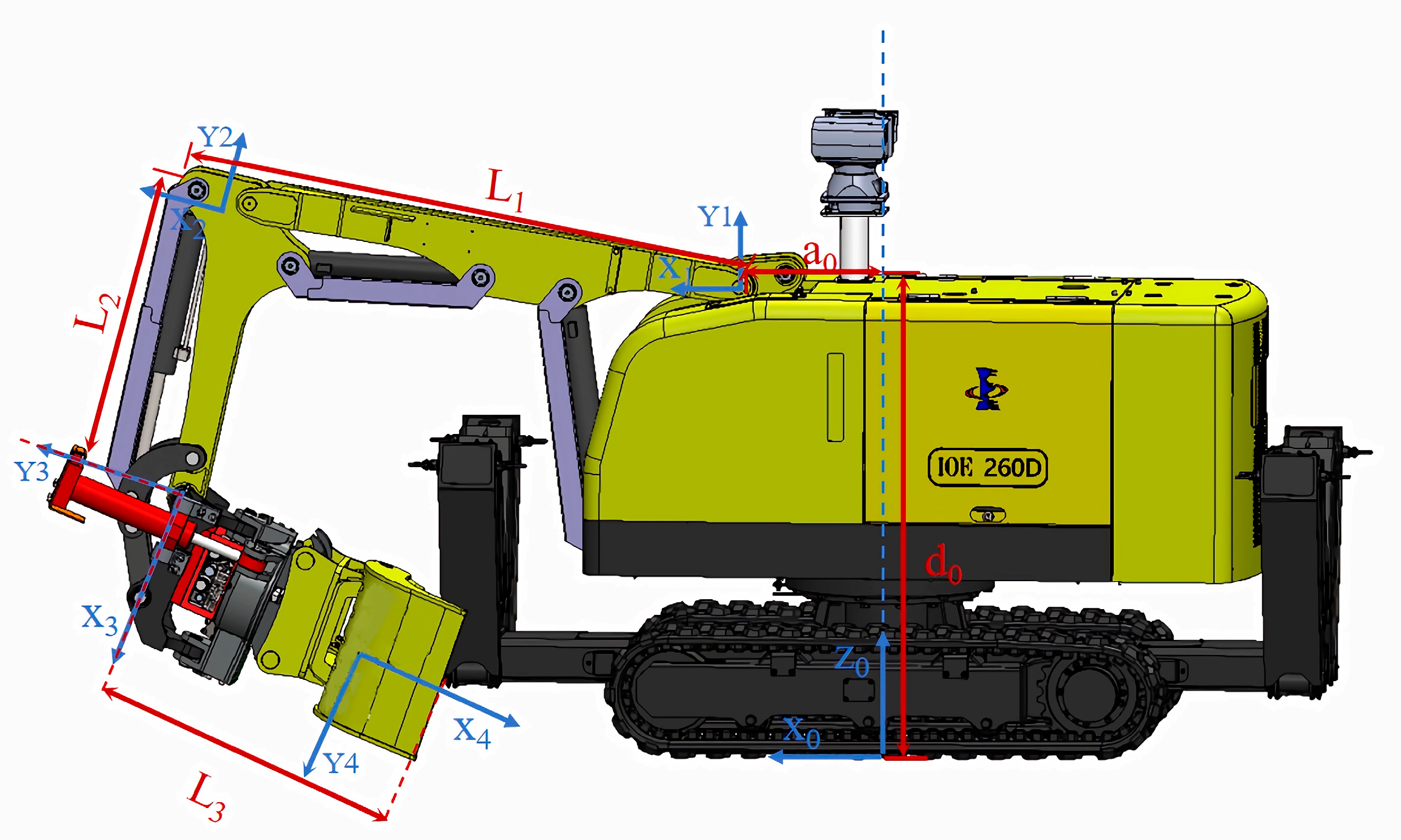
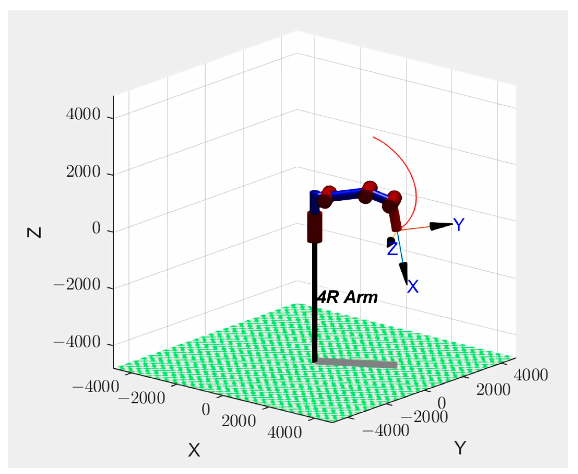
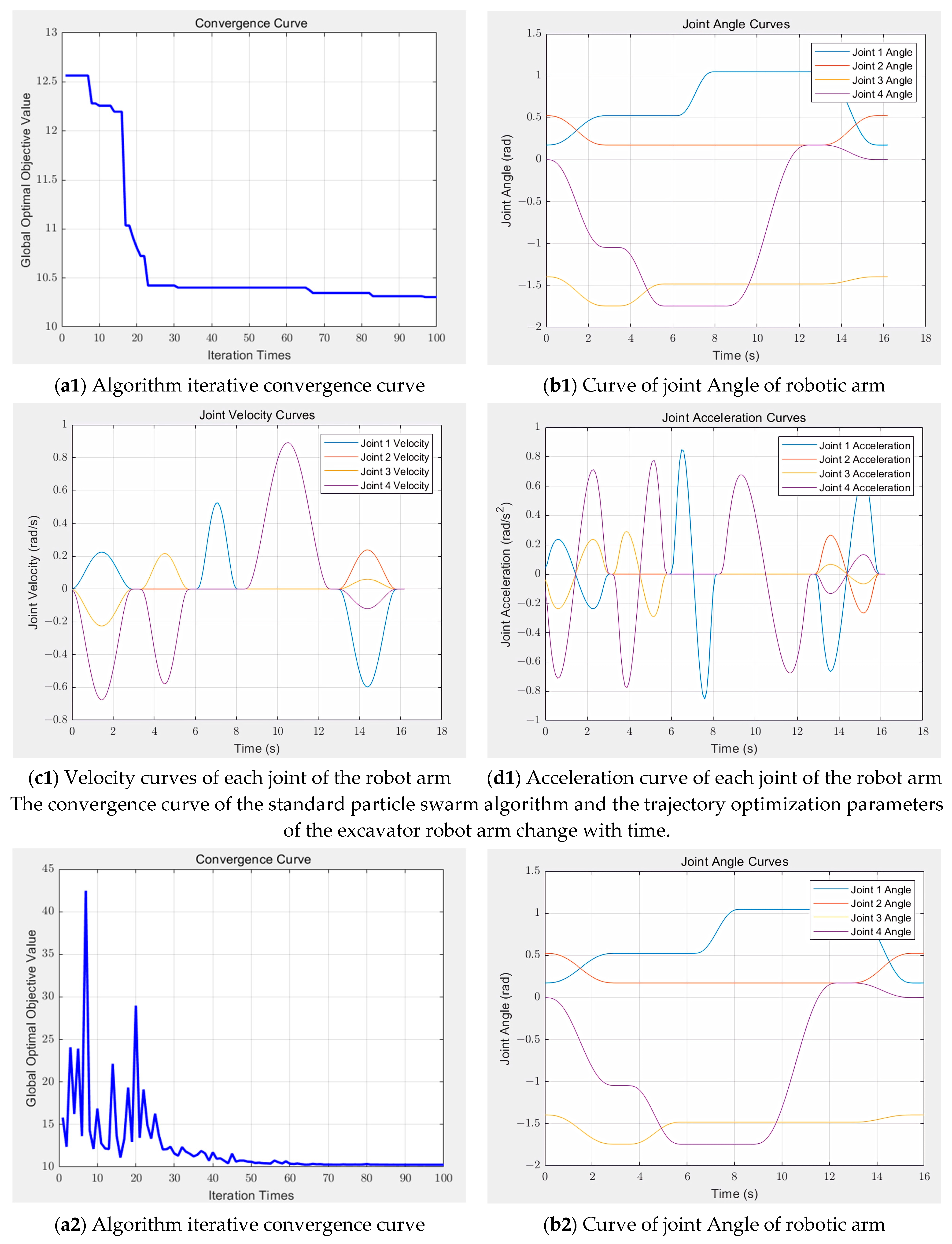
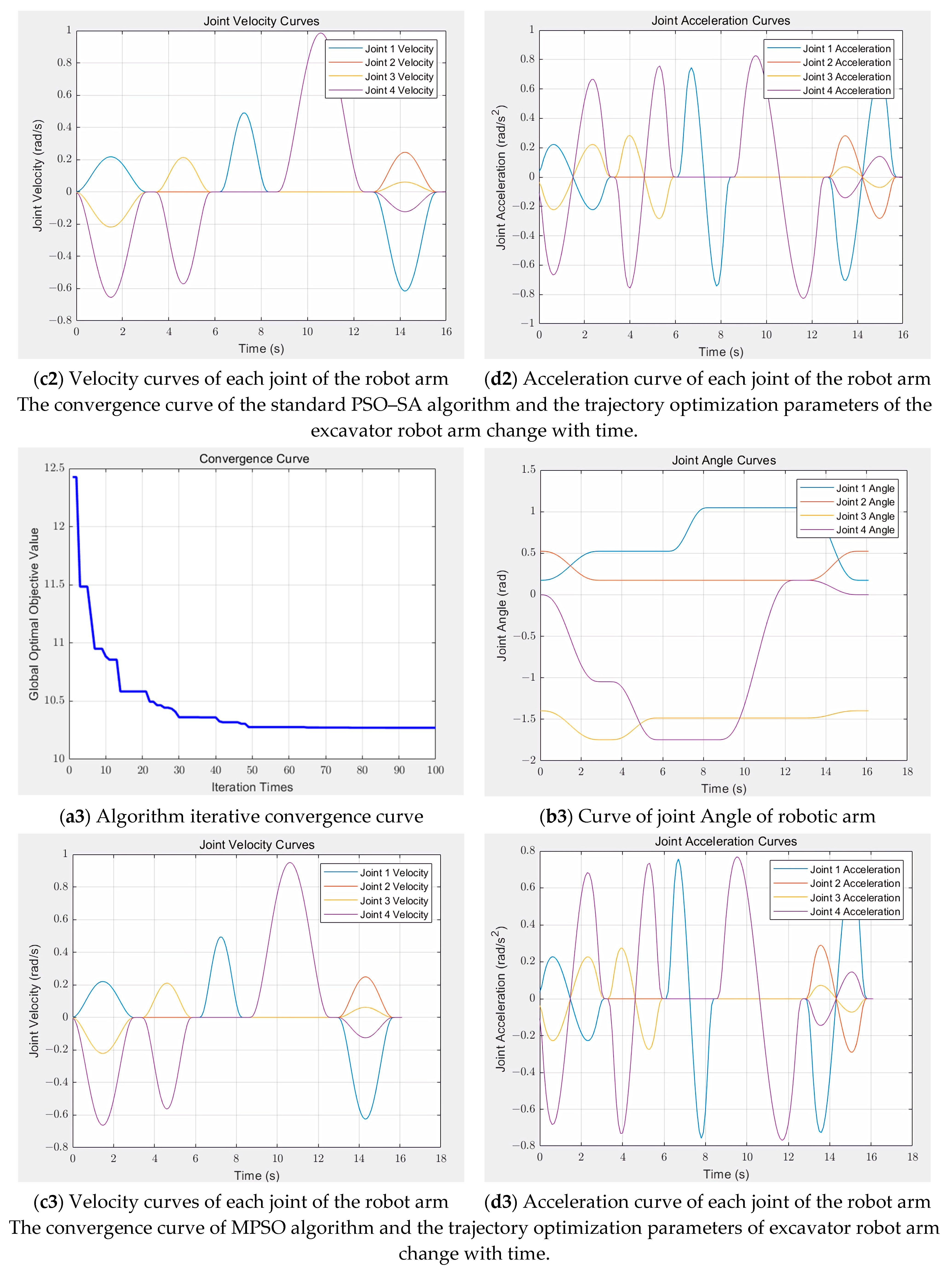
In this study, the improved PSO–SA optimization algorithm was used to plan the trajectory of the excavator manipulator arm with 4 degrees of freedom. The five-order B-spline curve was used to plan the trajectory in the joint space, and the improved PSO–SA algorithm was used to optimize the node vector of the trajectory planning of the five-stage operation task so that the excavator manipulator arm bucket completed a complete trajectory movement for the excavation task.

In this study, the simulated annealing algorithm and the particle swarm optimization algorithm are combined to improve the performance of the particle swarm optimization algorithm. The simulated annealing algorithm [24] is a stochastic optimization algorithm based on the physical annealing process, and its core idea is to simulate the physical phenomena in the annealing process of solid matter, allowing the algorithm to accept the better solution with a certain probability in the search process, so as to effectively avoid falling into the local optimal solution. In the simulated annealing process, the solid matter is heated to high temperatures and then cooled slowly, and the particles are more energetic at high temperatures and are able to move and rearrange freely. As the temperature gradually decreases, the particles gradually tend to a low-energy steady state. The simulated annealing algorithm draws on this process to continuously find the global optimal solution of the objective function in the search space, which provides an effective improvement strategy for the particle swarm optimization algorithm, helpful in improving its global optimization ability and search efficiency.

PSO–SA improves several aspects compared to standard PSO in global search capability and the avoidance of precocious convergence and convergence speed. Firstly, the inertia weight ω is adjusted by random generation, and the learning factors $c_1$ and $c_2$ are adjusted according to the progress ratio of the iteration, $c_1$ decreases linearly with the increase in the progress ratio, $c_2$ gradually increases with the increase in the progress ratio, and $c_1$ gradually decreases and $c_2$ gradually increases with the progress of the iteration, which helps to enhance the global search ability of particles in the early stage and improve the local search accuracy of particles in the later stage. This dynamic adjustment strategy not only improves the global search ability of the algorithm, but also enhances the convergence speed and the quality of the solution. Secondly, diversity monitoring was used for particle populations and, when the diversity was below the threshold, some particles were reset to avoid premature convergence. Combined with the perturbation mechanism of SA, some particles are randomly perturbed, the new solution is accepted according to the Metropolis criterion, and the global search ability is enhanced to balance the exploration and development capabilities. The cooling rate and perturbation ratio of SA are dynamically adjusted according to the ratio of the accepted solution so that the algorithm can adapt according to the search situation and balance global search and local search capabilities. The individual learning factor ranges from 1.0 to 2.0, with higher values in the early stages, leading particles to overly rely on their own experience and become trapped in local regions. As the individual learning factor decreases, particles gradually balance their own and collective experiences, thus expanding the search scope and increasing the likelihood of finding the global optimal solution. The social learning factor is set between 1.0 and 2.5, with lower values in the initial phase, which helps maintain diversity and prevent premature convergence. This gradually increases later on to enhance global search capabilities. The inertia weight [25] is controlled within the range of 0.6 to 0.8, avoiding both the weakening of global search capabilities due to too low values and the slowing down of convergence or solution domain oscillation caused by excessively high values. The initial population size is set at 50, ensuring algorithm efficiency while keeping computational costs within a reasonable range. One hundred iterations can achieve stable convergence, fully exploring the search space while avoiding resource wastage. In the simulated annealing phase, the initial temperature is set to 350 to enhance early global exploration, the termination temperature is 1 × 10⁻³ to ensure high solution domain accuracy later on, the initial cooling rate is 0.98 to balance global exploration with local development, and the perturbation ratio is 0.2 to control the local disturbance amplitude of particles, maintaining solution domain stability. Here are the main elements of the algorithm improvements:

(1)

Dynamically update the inertia weight $\omega$, learning factors $c_1$ and $c_2$

Randomly generate adjusted inertia weights, where ${\omega }_{max}$ and ${\omega }_{min}$ are the maximum and minimum weight values, respectively:

$$\omega ={\omega }_{\min }+({\omega }_{\max }-{\omega }_{\min })\times rand()$$

(19)

The learning factors c₁ and c₂ adopt an exponential dynamic adjustment strategy, c_1s is the initial individual learning factor, c_2S is the initial social learning factor, c_2e is the final social learning factor, $p_r$ is the iteration progress ratio, ITER is the current number of iterations, Max-Iter is the maximum number of iterations, and the range of rand () is between [0, 1].

$$\left\{\begin{array}{c}{p}_r={({\displaystyle \frac{iter}{\max -iter}})}^{1.5}\\ c_1=c_{1s}\times e^{-3p_r}\\ c_2=c_{2s}+(c_{2e}-c_{2s})\times (1-e^{-3p_r})\end{array}\right.$$

(20)

(2)

The diversity of particle swarms is calculated by Euclidean distance:

$$d={\displaystyle \frac{1}{n}}{\displaystyle \sum _{i=1}^n\sqrt{{\displaystyle \sum _{j=1}^d{(x_{i,j}-{\mu }_j)}^2}}}$$

(21)

where: n is the number of particles, d is the dimension, x_i,j is the position of the particles i on the dimension j, and μ_j is the mean of all the particles in the dimension j.

(3)

The SA parameters are adaptively adjusted, where $C_r$ is the cooling rate, $p_s$ the perturbation ratio, $A_r$ the acceptance rate of the new solution, and T is the temperature update formula in each iteration. In order to ensure that the improved algorithm maintains high temperature enhancement exploration in the early stage, and rapid cooling strengthens the development in the later stage, T is adaptively adjusted after each iteration:

$$C_r=\left\{\begin{array}{l}\min (C_r\times 1.02,0.995)\\ \max (C_r\times 0.98,0.9)\end{array}\right.\begin{array}{c}{A}_r>0.4\\ A_r<0.2\end{array}$$

(22)

$$P_s=P_s\times (0.8+0.4\times A_r)$$

(23)

$$T=\max (T\times C_r,T_{end})$$

(24)

$$\left\{\begin{array}{cc}T=T\_init\times ({\displaystyle \frac{1-iter}{\max \_iter\times 0.3}})& iter<\max \_iter\times 0.3\\ T=T\_init\times 0.3\times (1-{\displaystyle \frac{iter-\max \_iter\times 0.3}{\max \_iter\times 0.7}})& iter\ge \max \_iter\times 0.3\end{array}\right.$$

(25)

(4)

Simulated annealing algorithm in the original solution $E_{\left(x_i\right)}.$ The neighborhood randomly generates a new solution by perturbating $E_{\left(x_{i\_new}\right)}$. The Metropolis criterion determines the probability of accepting a new solution in simulated annealing [26], and the rand() range is between [0, 1]:

$$p=\left\{\begin{array}{c}1\\ \exp (-{\displaystyle \frac{\Delta E}{T\times (1+0.5rand())}})\end{array}\begin{array}{c}\Delta E<0\\ \Delta E\ge 0\end{array}\right.$$

(26)

$$\Delta E=E(x_{i\_new})-E(x_i)$$

(27)

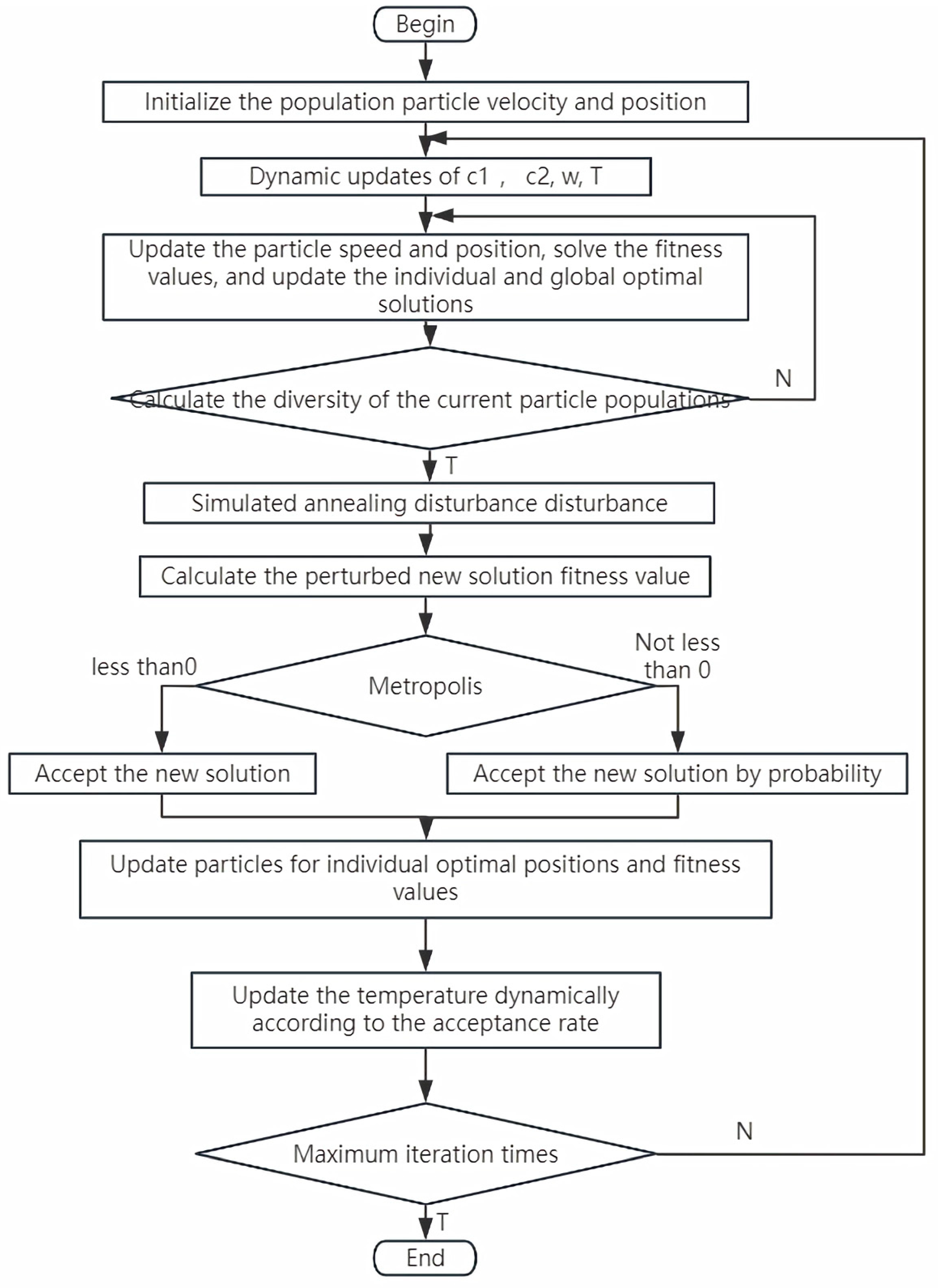
Here are the specific steps to improve the PSO algorithm. The specific flow chart is shown in Figure 5.

(1) The initial parameters are set as follows: the inertia weight range for the PSO algorithm is set to 0.6–0.8, the individual learning factor range is 1.0–2.0, and the social learning factor range is 1.0–2.5. An initial population of 50 particles is randomly generated in the search space, with each particle representing five sets of node vector time parameters. The number of iterations is 100. For the SA algorithm, the initial temperature is 350, and the termination temperature is 1 × 10⁻³.

(2) Initialize the velocity and position of the particles in the population and set the initial position of m particles to the individual optimal position p_ib of each particle. Compare the magnitude of the fitness function value of m particles, and the position of the particle with the smallest fitness function value is set to the historical optimal position of the particle swarm g_b.

(3) The individual learning factor $c_1$ was calculated by Formula (19), the social learning factor $c_2$ was calculated by Formula (19), and the inertia weight ω was calculated by Formula (18) for the dynamic parameter update.

(4) Use the velocity update formula of PSO to update the velocity of the particles by combining the current particle position, individual optimal position, and global optimal position. Based on the updated velocity, the new position of the particle is calculated, and the position is within the set boundary. For each particle’s new position, the objective function is called to calculate its fitness value. The new fitness value is compared with the individual optimal fitness value of the particle and, if it is better, the individual optimal position and fitness value are updated. The individual optimal fitness value and the global optimal fitness value were further compared, and the global optimal position and fitness value were updated if it was better.

(5) Calculate the diversity of the current particle swarm and evaluate it by measuring the Euclidean distance between the particles and the population mean. If the diversity falls below the set threshold, the position and velocity of some particles are randomly reset to introduce new solutions and avoid premature convergence.

(6) If the diversity is greater than the set threshold, 40% of the individual historical optimal solutions (p_best) are randomly selected, the mixed stochastic strategy is used to simulate the annealing perturbation with Gaussian perturbation, a new candidate solution is generated, and the objective function is called to calculate the fitness value of the candidate solution, according to the Metropolis acceptance criterion. If the calculation is less than zero using Equation (25), the acceptance is forced, otherwise the acceptance probability is calculated, it is decided to accept the new solution and, if the new solution is better than g_best, the global optimal is updated.

(7) Dynamically adjust the cooling rate according to the search effect; if the acceptance rate of step (6) is greater than 40%, accelerate cooling; if the acceptance rate of step (6) is less than 20%, decelerate cooling, and use Equation (23) to calculate and update the temperature parameter T, so that it gradually decreases, and the simulated annealing process gradually converges.

(8) Judge whether the maximum number of iterations is reached, return to step (3) if it is not satisfied, and exit the loop if it is satisfied.

3. Results

3.1. Mining Task Analysis and Simulation Settings

In this study, a single excavation task for a certain type of unmanned excavator is planned continuously, and the main content of the excavation operation task is to start moving from the starting point A to the excavation point B, carrying out the excavation operation, transporting the material to the unloading point D for the unloading operation, and then returning to the origin point A; the single excavation operation process of the unmanned excavator is shown in

Table 4. Trajectory flow of the unmanned excavation operation.

The Point at Which the Trajectory Runs	The Name of the Action
A	The robotic arm is stationary
B	Material mining
C	Pit bucket lift
D	The working device rotates
E	Material unloading
A	Empty bowl turn

.

In order to verify the correctness and effectiveness of the improved PSO–SA algorithm in the continuous trajectory planning of a certain type of excavator manipulator in the laboratory, and to prove the advantages of convergence accuracy compared with other algorithms, this study compared it with the standard particle swarm algorithm, the multi-swarm particle swarm optimization algorithm and the standard particle swarm-simulated annealing algorithm. The simulation takes the time and energy consumption of trajectory planning as the objective function, and uses four different intelligent algorithms to optimize the continuous trajectory planning of a single mining task, the trajectory of each joint of the robotic arm is constructed by five B-spline curves, the sequence of various types of value points through each joint trajectory is shown in

Table 5. Excavation trajectory joint angle value points.

Joint Position	q/(°)
	1	2	3	4
A	10	30	−80	0
B	30	10	−100	−60
C	30	10	−8	−100
D	60	10	−85	−100
E	60	10	−85	10
A	10	30	−80	0

, and the angular velocity and angular acceleration of the start and stop of each joint trajectory are 0. The description of the simulation environment is as follows: (1) Computer software and hardware configuration, OS Windows 10; Processor Intel Core i7-10750H; Graphics NVIDIA GeForce GTX 1650 Ti. (2) Simulation software MATLAB 2020b.

3.2. Analysis of Simulation Results

The simulation results are shown in Figure 6, and the convergence curve of the standard PSO algorithm shows a rapid downward trend at the initial stage and tends to stabilize when the number of iterations reaches 20. However, the final convergence value is slightly higher than that of other improved algorithms, which indicates that the algorithm has some limitations in terms of optimization accuracy. Further observation showed that the change in joint angle was stable as a whole, but there was a slight overshoot. The velocity and acceleration curves exhibit significant fluctuations, which can adversely affect the smooth operation and precision control of the robotic arm. The convergence process of the standard PSO–SA algorithm shows violent fluctuations, which not only affects the optimization efficiency but also may make it difficult for the algorithm to stabilize quickly in practical applications. In addition, the joint angle under this algorithm also has the problem of overshooting, and the fluctuation amplitude of the velocity and acceleration curves is larger than that of the standard PSO algorithm. This characteristic means that higher requirements are placed on the dynamic performance of the robotic arm, otherwise it may not be conducive to the long-term stable operation of the robotic arm. In contrast, the MPSO algorithm shows a faster convergence speed, but its convergence value is between the standard PSO and the improved PSO–SA algorithm, indicating that its optimization accuracy and efficiency are at a medium level. In terms of the motion characteristics of the robotic arm, the joint angle curve under the MPSO algorithm is relatively smooth, the overshoot is small, the velocity fluctuation amplitude is relatively low, and the acceleration curve is relatively smooth. Nevertheless, there is room for further optimization of these metrics. The improved PSO–SA algorithm performs well in all aspects. Its convergence speed is not only fast and stable, but the change in joint angle is extremely stable, the speed curve is smooth, and the acceleration curve fluctuation is small, which can effectively avoid mechanical impact so as to ensure the long-term stable operation and high-precision operation of the robotic arm. On the whole, the improved PSO–SA algorithm has obvious advantages over other algorithms in many key indicators, such as convergence speed, trajectory accuracy, motion smoothness and mechanical life guarantee, and is a better choice for manipulator trajectory planning. The practical application of this algorithm will significantly improve the performance and operation quality of the robotic arm and provide reliable support for high-precision tasks in industrial production.

Figure 6 and Figure 7 show the trajectory of the operation in the Cartesian coordinate system using the improved PSO–SA algorithm for continuous trajectory planning of a single mining task. From the end trajectory curve, it can be seen that the intermediate process is continuous without obvious discontinuity, and the improved PSO–SA algorithm can generate a complete and coherent motion path. The trajectory is relatively smooth as a whole, and there is no sharp turning or abrupt change in most areas, which is conducive to the smooth operation of the robotic arm and reduces vibration and impact. The distribution of trajectories in space shows that the algorithm considers the kinematic constraints and working space constraints of the manipulator well, and the end effector can move flexibly in the predetermined area to meet the task requirements.

Table 6. Comparison of the simulation performance of four intelligent algorithms.

Algorithm	Maximum Fitness Value	Minimum Fitness Value	Standard Deviation	Time
MPSO	10.463	10.271	0.043	1155.886
Standard PSO–SA	10.359	10.270	0.017	1155.369
Improvement of PSO–SA	10.570	10.269	0.047	2315.602
PSO	11.605	10.305	0.300	973.291

and

Table 7. Results of trajectory optimization for four intelligent algorithms.

Time	MPSO	Standard PSO–SA	Improvement of PSO–SA	PSO
T1	2.952	2.989	2.941	2.892
T2	2.313	2.279	2.314	2.248
T3	1.966	1.983	1.932	1.847
T4	3.780	3.643	3.713	4.031
T5	2.606	2.647	2.633	2.728
T total	13.617	13.541	13.533	13.746

show the comparison between the simulation performance results and optimization results for four intelligent algorithms, and analyze Table 6 and Table 7. The MPSO algorithm has excellent performance in terms of computing speed, can complete the optimization task in a short time, and its fitness value fluctuates little, which indicates that the algorithm has good stability in the optimization process, and it can quickly obtain the solution while ensuring a certain optimization effect, which is suitable for situations with high requirements for time efficiency and a small problem scale. The standard PSO–SA algorithm has a balanced performance in the fluctuation control and time consumption of fitness values, which not only has a certain stability, but can also avoid large fluctuations in the solution to a certain extent, but can also complete the optimization task within an acceptable time range, and has considerable efficiency. The calculation time of the PSO algorithm is the shortest among the three algorithms, and the preliminary solution can be obtained in a very short time, which is suitable for simple problems that do not require high optimization accuracy and need to obtain the preliminary solution quickly. However, its fitness value fluctuates greatly, and the stability of the optimization results is not good, which may produce large differences in different runs. Comprehensive comparative analysis shows that the improved PSO–SA algorithm performs best in terms of stability of fitness value and accuracy of optimization results. Although it consumes relatively more time, this investment is worthwhile for precise operations. The algorithm can effectively balance the stability and optimization accuracy of the algorithm, making it suitable for complex and refined tasks with high requirements for optimization quality.

3.3. Discussion

This paper presents an improved PSO–SA algorithm designed for unmanned excavator operation scenarios. The gap between the maximum and minimum fitness values of this algorithm is significantly smaller than that of other algorithms. This indicates that the algorithm has a clear advantage in terms of accuracy, providing more precise path planning and operational control parameters for unmanned excavators. However, this performance improvement comes with a significant increase in run time. In the selection and application of algorithms, a comprehensive trade-off must be made based on specific task types and precision requirements. For complex and detailed tasks, the high-precision characteristics of the improved PSO–SA algorithm can ensure task quality and effectiveness, while its longer run time can be mitigated through optimizing algorithm parameters, enhancing hardware performance, or adopting parallel computing. For simple, repetitive tasks with extremely high real-time requirements, we reduce the number of iterations and appropriately adjust the precision target of the algorithm to prioritize rapid decision-making while ensuring basic task quality. At the same time, this study primarily focuses on analyzing and validating algorithms and strategies related to unmanned excavators based on simulation models. Although the simulation platform has advantages, such as efficiency and controllability in theoretical derivation, concept validation, and preliminary optimization, capable of quickly simulating various working conditions and providing critical data support, the research team also fully recognizes that relying solely on simulations has limitations due to differences from actual hardware environments. Some complex physical characteristics, hardware response delays, and real-world interference factors cannot be accurately replicated. In response to this situation, this study plans to conduct experimental verification work based on physical unmanned excavators. By comparing simulation results with experimental results, the effectiveness of the algorithms in practical applications will be verified, and the research findings will be promoted and applied to a broader range of unmanned excavator application scenarios.

4. Conclusions

In this paper, aiming at the problem of single-time continuous operation trajectory planning of unmanned excavators, considering the minimum comprehensive time and energy consumption of the excavator manipulator operation trajectory as the objective function, the five-order B-spline curve is used for trajectory planning, and an intelligent hybrid algorithm with improved PSO algorithm and simulated annealing algorithm is designed to optimize trajectory planning. According to the comparative analysis of the simulation results, the improved PSO–SA algorithm shows significant advantages over other algorithms in the research on manipulator trajectory optimization. The algorithm can converge to the global optimal solution faster, and the generated trajectory has higher tracking accuracy. By optimizing the nodal vector of the fifth B-spline curve, the joint motion curve obtained is continuous and smooth, without step mutation, which effectively inhibits the rigid and flexible impact of the manipulator in motion. In addition, the improved PSO–SA algorithm also shortens the running time of the robotic arm, verifies its feasibility, superiority, and effectiveness in the trajectory planning of the robotic arm, and provides a reliable method for high-precision and high-efficiency robotic arm motion control.

References

1. Fu, T.; Hu, Z.; Zhang, T.; Bi, Q.; Song, X. Physics-Informed Neural Networks-Based Online Excavation Trajectory Planning for Unmanned Excavator. Chin. J. Mech. Eng. 2024, 37, 131. [Google Scholar] [CrossRef]
2. Zhang, T.; Fu, T.; Ni, T.; Yue, H.; Wang, Y.; Song, X. Data-driven excavation trajectory planning for unmanned mining excavator. Autom. Constr. 2024, 162, 105395. [Google Scholar] [CrossRef]
3. Shengxi, L. Robot Trajectory Planning and Simulation Based on Matlab Robotics Toolbox. J. Artif. Intell. Pract. 2024, 7, 90–100. [Google Scholar]
4. Potter, H.; Kern, J.; Gonzalez, G.; Urrea, C. Energetically optimal trajectory for a redundant planar robot by means of a nested loop algorithm. Elektron. Elektrotechnika 2022, 28, 847–856. [Google Scholar] [CrossRef]
5. Sun, X.; He, S.; Xu, Z.; Zhang, E.; Li, Y. Research on Configuration Design Optimization and Trajectory Planning of Manipulators for Precision Machining and Inspection of Large-Curvature and Large-Area Curved Surfaces. Micromachines 2023, 14, 886. [Google Scholar] [CrossRef]
6. Liu, J.; Huang, H.; Fan, Q.; Ma, C.; Zhang, L. Multi-objective trajectory planning of robotic arms based on improved salp swarm algorithm. China Mech. Eng. 2024, 51, 847. Available online: https://kns.cnki.net/kcms/detail/42.1294.th.20241031.1351.007.html (accessed on 1 November 2024).
7. Bi, Q.; Wang, G.; Wang, Y.; Yao, Z.; Hall, R. Digging trajectory optimization for cable shovel robotic excavation based on a multi-objective genetic algorithm. Energies 2020, 13, 3118. [Google Scholar] [CrossRef]
8. Zhang, H.; Li, L. An Improved Ant Colony for Servo Mechanical Arm Path Planning. In Proceedings of the 2015 International Conference on Intelligent Systems Research and Mechatronics Engineering; 2015; pp. 1447–1450. [Google Scholar]
9. Jichun, W.; Zhaiwu, Z.; Yongda, Y.; Ping, Z.; Dapeng, F. Time optimal trajectory planning of robotic arm based on improved tuna swarm algorithm. Comput. Integr. Manuf. Syst. 2024, 30, 4292. [Google Scholar]
10. Zacharia, P.T.; Xidias, E.K. Optimal robot task scheduling in cluttered environments considering mechanical advantage. Robotica 2024, 42, 3230–3246. [Google Scholar] [CrossRef]
11. Xidias, E.K. Time-optimal trajectory planning for hyper-redundant manipulators in 3D workspaces. Robot. Comput. -Integr. Manuf. 2018, 50, 286–298. [Google Scholar] [CrossRef]
12. Corke, P.I. A simple and systematic approach to assigning Denavit–Hartenberg parameters. IEEE Trans. Robot. 2007, 23, 590–594. [Google Scholar]
13. Prada, E.; Srikanth, M.; Miková, L.; Ligušová, J. Application of Denavit Hartenberg method in service robotics. Int. J. Adv. Robot. Syst. 2020, 5, 47–52. [Google Scholar]
14. Gasparetto, A.; Boscariol, P.; Lanzutti, A.; Vidoni, R. Path planning and trajectory planning algorithms: A general overview. In Motion and Operation Planning of Robotic Systems: Background and Practical Approaches; Springer: Berlin/Heidelberg, Germany, 2015; pp. 3–27. [Google Scholar]
15. Jia, L.; Zeng, S.; Feng, L.; Lv, B.; Yu, Z.; Huang, Y. Global Time-Varying Path Planning Method Based on Tunable Bezier Curves. Appl. Sci. 2023, 13, 13334. [Google Scholar] [CrossRef]
16. Jinqi, C.; Xuesong, H. Review of research methods for industrial robot trajectory planning. Inf. Control 2024, 53, 471–486. [Google Scholar]
17. Lu, L.; Zhang, L.; Fan, C.; Wang, H. High-order joint-smooth trajectory planning method considering tool-orientation constraints and singularity avoidance for robot surface machining. J. Manuf. Process. 2022, 80, 789–804. [Google Scholar]
18. Saeed, M.; Demasure, T.; Hoedt, S.; Aghezzaf, E.-H.; Cottyn, J. Spline-based trajectory generation to estimate execution time in a robotic assembly cell. Int. J. Adv. Manuf. Technol. 2022, 121, 6921–6935. [Google Scholar] [CrossRef]
19. Sun, H.; Tao, J.; Qin, C.; Dong, C.; Xu, S.; Zhuang, Q.; Liu, C. Multi-objective trajectory planning for segment assembly robots using a B-spline interpolation-and infeasible-updating non-dominated sorting-based method. Appl. Soft Comput. 2024, 152, 111216. [Google Scholar] [CrossRef]
20. Lu, Z.; You, Z.; Xia, B. Time optimal trajectory planning of robotic arm based on improved sand cat swarm optimization algorithm. Appl. Intell. 2025, 55, 1–54. [Google Scholar] [CrossRef]
21. Kuo, P.-H.; Syu, M.-J.; Yin, S.-Y.; Liu, H.-H.; Zeng, C.-Y.; Lin, W.-C.; Yau, H.-T. Intelligent optimization algorithms for control error compensation and task scheduling for a robotic arm. Int. J. Intell. Robot. Appl. 2024, 8, 334–356. [Google Scholar] [CrossRef]
22. Wang, T. Trajectory Optimization and Control of Grinding Robot Based on Improved Whale Optimization Algorithm. Ph.D. Thesis, North University of China Taiyuan, Taiyuan, China, 2021. [Google Scholar]
23. Ang, K.; Yeap, Z.; Chow, C.; Cheng, W.; Lim, W. Modified Particle Swarm Optimization with Chaotic Initialization Scheme for Unconstrained Optimization Problems. Mekatronika J. Intell. Manuf. Mechatron. 2021, 3, 35–43. [Google Scholar]
24. Kirkpatrick, S.; Gelatt Jr, C.D.; Vecchi, M.P. Optimization by simulated annealing. science 1983, 220, 671–680. [Google Scholar] [CrossRef] [PubMed]
25. Nickabadi, A.; Ebadzadeh, M.M.; Safabakhsh, R. A novel particle swarm optimization algorithm with adaptive inertia weight. Appl. Soft Comput. 2011, 11, 3658–3670. [Google Scholar] [CrossRef]
26. Turhan, A.M.; Bilgen, B. A hybrid fix-and-optimize and simulated annealing approaches for nurse rostering problem. Comput. Ind. Eng. 2020, 145, 106531. [Google Scholar] [CrossRef]
Figure 1. Structural diagram of an unmanned excavator.
Actuators 14 00226 g001
Figure 2. D–H coordinate system of the unmanned excavator manipulator. The blue solid arrow indicates the coordinate axis, the blue dashed line is the auxiliary line, the red solid arrow indicates the length parameter, and the red dashed line is the auxiliary line.
Actuators 14 00226 g002
Figure 3. Trajectory planning trajectory of the robotic arm. The arrow indicates the end coordinate axis, the red solid line indicates the motion trajectory, the red cylinder indicates the joint of the robot arm, and the blue cylinder indicates the connecting rod of the robot arm.
Actuators 14 00226 g003
Figure 4. Simulation results of three trajectory planning methods.
Actuators 14 00226 g004
Figure 5. Flow chart of the improved particle swarm algorithm.
Actuators 14 00226 g005
Figure 6. Trajectory optimization simulation results of four algorithms.
Actuators 14 00226 g006aActuators 14 00226 g006bActuators 14 00226 g006c
Figure 7. Tracing simulation of the excavator robot arm. The arrows indicate the coordinate axis, and the blue solid line indicates the trajectory.
Actuators 14 00226 g007