Fast Dynamic P-RRT*-Based UAV Path Planning and Trajectory Tracking Control Under Dense Obstacles

Abstract

This work develops an improved integrated planning and control framework for an unmanned aerial vehicle (UAV) in complex environments with dense obstacles to achieve fast and accurate path planning, trajectory generation, and tracking control. Utilizing the potential function-based rapid-exploration random tree star (P-RRT*), a bidirectional dynamic informed P-RRT* (BDIP-RRT*) algorithm is first introduced to enhance sampling efficiency, facilitating swift path generation. To further optimize the initial path, a greedy algorithm is employed to minimize redundant segments within the generated path. Subsequently, trajectory control points are assigned based on the original path points using an adaptive distance interpolation strategy. A hybrid optimized trajectory generator considering jerk and snap is built to obtain a reference trajectory for the UAV. Moreover, two prescribed-time control laws are designed to ensure fast and accurate UAV position and attitude control. Finally, simulation results are performed to illustrate the effectiveness and superior performances of the developed path planning and control scheme.

1. Introduction

In recent decades, UAVs have become increasingly popular owing to their cost-effectiveness and operational efficiency, making them prevalent in tasks such as safety inspection, terrain survey, search and rescue, and more [1,2,3]. The pivotal capability enabling UAVs to achieve these missions is autonomous flight, including perception, decision-making, planning, and control [4,5]. More particularly, the path planning and control methods play decisive roles in the execution of the flight missions. However, the UAV planning and control systems that are designed independently cannot coordinate effectively in complex environments with dense obstacles, such as urban infrastructure, forested areas, or other similarly dense obstacle environments. The planning system may generate paths that are difficult to execute smoothly, while the control system may struggle to meet the requirements deriving from the planning system. Therefore, integrated frameworks for planning and control are of paramount importance in addressing these challenges effectively for UAV under dense obstacles.

UAV path planning techniques based on configuration space are primarily categorized into graph search methods, sampling-based methods, optimization-based methods, and intelligent algorithms [6,7,8]. When dealing with maps of larger scales, sampling-based methods exhibit noticeably higher efficiency compared with other methods [9]. In sampling-based methods, the probabilistic road map (PRM) algorithm is adept at covering path planning, while the RRT algorithm excels at exploring paths. PRM tends to generate numerous nodes, leading to increased computational cost, whereas RRT solves this by swiftly expanding randomized search trees. Bi-RRT [10] and RRT-Connect [11] efficiently generate two trees from the initial and target points until they become connected. These algorithms accelerate the path generation speed of RRT by optimizing the tree structure. Karama et al. [12] addressed the issue of low path quality when exploring high-dimensional spaces and proposed the RRT* algorithm to improve the quality of the generated path by introducing a cost function and optimization strategy. Informed RRT* was presented in [13] to reduce the number of invalid sampling points by employing hyperspheroid subsets to constrain the sampling region, whereas the P-RRT* algorithm improves the convergence speed and memory efficiency of RRT* by incorporating the artificial potential field approach [14]. Quick-RRT* accelerates convergence to the optimal solution by expanding the set of possible parent vertices, leading to paths with lower cost [15]. GMR-RRT* utilizes probabilistic modeling to integrate Gaussian mixture regression with RRT*, achieving fast and high-quality path planning through efficient learning from human demonstrations and guided sampling [16]. In addition, PIB-RRT* [17], PQ-RRT* [18], AEB-RRT* [19], and some other hybrid algorithms can further improve the quality and efficiency of path generation based on the above-mentioned algorithms.

UAV path planning algorithms typically generate discrete waypoints without incorporating dynamic constraints or time allocation, which induces abrupt changes in control inputs and consequently results in discontinuities in velocity and acceleration during execution [20,21]. Therefore, trajectory generation and optimization are necessary for UAVs in complex 3D spatial environments. Trajectory optimization necessitates specifying three components: curve description modes, optimization objectives, and constraint methods. Curve description modes for the trajectory include polynomial curves, Bezier curves, spline curves, etc. [22,23,24]. The trajectory optimization objective refers to the performance metric quantifying the extent to which the specified objectives set by the designer can be achieved given a predefined task overview and a large set of feasible flight trajectory collections [25]. In trajectory constraint methods, hard constraints are strict conditions that must be met during optimization, while soft constraints are desired but not mandatory [26]. Following Mellinger et al.’s introduction of Minimum Snap [27], Brown et al. [28] proposed a UAV trajectory optimization method utilizing a fifth-order polynomial to minimize power consumption, maximize the average probability of detection, and minimize the average revisit time. To ensure smooth flight paths and maintain curvature continuity, Hu et al. [29] designed a 3D B-spline template to minimize the path curvature. By employing a line-of-sight path optimizer to insert additional waypoints into planned straight-line segments, Woo et al. [30] ensured a smooth position and heading angle by using a spline trajectory generator and referencing a prescribed velocity distribution for the flyable trajectory.

Even with path planning and trajectory optimization, the trajectory tracking control of UAVs presents another challenge due to the inherent strong coupling and underdrive characteristics along with complex uncertainties. Proportional integral derivative (PID) control is practical and often applied to full six-degree-of-freedom control of UAVs [31]. However, PID controllers can only achieve asymptotic stability, and are sensitive to both external disturbances and system uncertainties. Therefore, researchers have proposed a series of nonlinear control schemes, including active disturbance rejection control (ADRC) [32], backstepping control (BSC) [33], sliding mode control (SMC) [34], etc. Xu et al. [35] cascaded the ADRC and backstepping SMC schemes to process attitude and position subsystems, demonstrating effectiveness, robustness, and practical feasibility. It should be noted that finite/fixed-time control schemes have been given more attention recently due to their superior performances of fast convergence, fine stabilization, and strong robustness. In [36], a distributed fixed-time estimator was proposed to estimate the leader’s position and velocity information within a fixed stable time and without the use of initial conditions. To achieve precise trajectory tracking under various disturbance conditions, Li et al. [37] proposed a fixed-time velocity control law and fixed-time trajectory tracking control law integrating a fast fixed-time disturbance observer. However, the above finite/fixed-time control schemes can not support pre-assignment of the convergence time. Gong et al. [38] presented a prescribed-time fault-tolerant tracking control with pre-assigned convergence time for quadrotor UAVs.

In view of the above results, although UAV path planning, optimized trajectory generation, and trajectory tracking control have undergone extensive relevant investigation individually, integrated designs are currently lacking for missions with diverse and complex environments. Although the path planning algorithm in [9] is designed for specific environments, it does not consider adaptability in the design of trajectory generation and tracking control, resulting in a lack of overall system coherence. The integrated design in [30] lacks unified optimization objectives and coordination mechanisms, resulting in weak system integration with insufficient coherence and consistency between modules. Thus, in this work we propose an integrated fast planning and control scheme design method for UAVs in environments with dense obstacles, offering the following main contributions:

(1)

A fast bidirectional dynamic informed P-RRT* (BDIP-RRT*) algorithm is first developed for UAV in dense obstacle environments. Superior to the P-RRT* algorithm [14], the bidirectional dynamic informed structure is optimized in terms of sampling probability, sampling range, target bias, and a multi-tree structure to improve the quality and speed of initial path generation.

(2)

A hybrid optimized trajectory generator is proposed that significantly improves trajectory smoothness and efficiency by optimizing jerk and snap compared with the spline-based method in [30]. More specifically, an adaptive distance interpolation strategy is introduced to generate trajectory control points, further balancing control performance and trajectory deviation.

(3)

Two prescribed-time control laws are designed to ensure fast and accurate UAV position and attitude control. A segmented function is introduced in the prescribed-time control laws to suppress the growth of the scale function and solve the singularity-like problem [39].

2. Preliminaries and Problem Statement

Before introducing the integrated planning and control system design framework, it is essential to establish the mathematical model of the UAV. The inertial frame is denoted as $O_I$-$X_I{Y}_I{Z}_I$, while $O_B$-$X_B{Y}_B{Z}_B$ is the body’s fixed frame established with the UAV’s center of mass. To characterize the UAV’s position and attitude in the inertial frame, the center position is denoted as $\mathit{X}={[x,y,z]}^{\mathrm{T}}$ and the attitude is represented by Euler angles $\mathbf{\Theta }={[\varphi ,\theta ,\psi ]}^{\mathrm{T}}$, where $\varphi$, $\theta$, and $\psi$ denote the roll, pitch, and yaw angles, respectively. Then, the dynamics of the disturbance-free system with an inertia matrix of $\mathit{I}=\mathrm{diag}\left\{{[I_{11},I_{22},I_{33}]}^{\mathrm{T}}\right\}$ can be established as follows  [40]:

$$m\ddot{\mathit{X}}+mg{\mathit{z}}_I=\mathit{R}\left(\mathbf{\Theta }\right)\mathit{U}$$

(1)

$$\mathit{J}\left(\mathbf{\Theta }\right)\ddot{\mathbf{\Theta }}+\mathit{C}(\mathbf{\Theta },\dot{\mathbf{\Theta }})\dot{\mathbf{\Theta }}=\mathit{\tau }$$

(2)

where $m\in {\mathbb{R}}^{+}$ is the total mass of the UAV, $g\in {\mathbb{R}}^{+}$ is the acceleration of gravity, and ${\mathit{z}}_I$ is a unit vector with ${\mathit{z}}_I={[0,0,1]}^{\mathrm{T}}$. The rotation matrix $\mathit{R}\left(\mathbf{\Theta }\right)\in {\mathbb{R}}^{3\times 3}$ describes the transformation relationship between the frames $O_I$-$X_I{Y}_I{Z}_I$ and $O_B$-$X_B{Y}_B{Z}_B$, which is presented as

$$\mathit{R}\left(\mathbf{\Theta }\right)=\left[\begin{array}{ccc}{b}_{11}& b_{12}& b_{13}\\ b_{21}& b_{22}& b_{23}\\ b_{31}& b_{32}& b_{33}\end{array}\right]$$

(3)

with $b_{11}=C\psi C\theta$, $b_{12}=C\psi S\theta S\varphi -S\psi C\varphi$, $b_{13}=C\psi S\theta C\varphi +S\psi S\varphi$, $b_{21}=S\psi C\theta$, $b_{22}=S\psi S\theta S\varphi +C\psi C\varphi$, $b_{23}=S\psi S\theta C\varphi -C\psi S\varphi$, $b_{31}=-S\theta$, $b_{32}=C\theta S\varphi$, and $b_{33}=C\theta C\varphi$. Here, $S·$ and $C·$ respectively denote the sine function $sin(·)$ and cosine function $cos(·)$. The thrust vector $\mathit{U}={[0,0,F]}^{\mathrm{T}}$ is defined in the body frame, where F represents the total thrust generated by the four motors. In addition, $\mathit{u}=\mathit{R}\left(\mathbf{\Theta }\right)\mathit{U}\in {\mathbb{R}}^3$ is the total translational force and $\mathit{\tau }\in {\mathbb{R}}^3$ is the total control torque for rotational motion, while $\mathit{J}\left(\mathbf{\Theta }\right)$ is a symmetric matrix

$$\mathit{J}\left(\mathbf{\Theta }\right)=\left[\begin{array}{ccc}{J}_{11}& 0& J_{13}\\ 0& J_{22}& J_{23}\\ J_{13}& J_{23}& J_{33}\end{array}\right]$$

(4)

with $J_{11}=I_{11}$, $J_{13}=-I_{11}S\theta$, $J_{22}=I_{22}{C}^2\varphi +I_{33}{S}^2\varphi$, $J_{23}=(I_{22}-I_{33})C\varphi S\varphi C\theta$, and $J_{33}=I_{11}{S}^2\theta +I_{22}{S}^2\varphi C^2\theta +I_{33}{C}^2\varphi C^2\theta$. The matrix $\mathit{C}(\mathbf{\Theta },\dot{\mathbf{\Theta }})\in {\mathbb{R}}^{3\times 3}$ is the Coriolis term of the UAV [40].

To construct an improved integrated path planning and control design framework, we utilize the aforementioned UAV mathematical model, as illustrated in Figure 1. First, a novel path planning algorithm is developed by employing P-RRT* in conjunction with a bidirectional dynamic informed structure and greedy algorithm to obtain a sequence of discrete points characterized by three-dimensional coordinates $(x_i,y_i,z_i)$ and yaw angles ${\psi }_i$, with $i=1,2,\dots ,N$. Due to the differential flatness property of UAVs, any smooth trajectory in three-dimensional space can be represented by $(x_i,y_i,z_i,{\psi }_i)$ [27]. Subsequently, a new hybrid optimized trajectory generator converts discrete path points into trajectory containing data such as time, velocity, and acceleration, namely, ${\mathit{X}}_d$ and ${\psi }_d$. Finally, prescribed-time position and attitude control laws are designed to achieve fast trajectory tracking control.

Unlike the integrated frameworks in [9,30], the proposed planning and control framework in this work is characterized by a unified optimization goal, namely, improving UAV motion performances within dense obstacle environments. Path planning aims to enhance the speed and quality of path generation, while trajectory generation focuses on producing smooth trajectory optimized for jerk and snap; finally, tracking control ensures rapid and stable trajectory tracking.

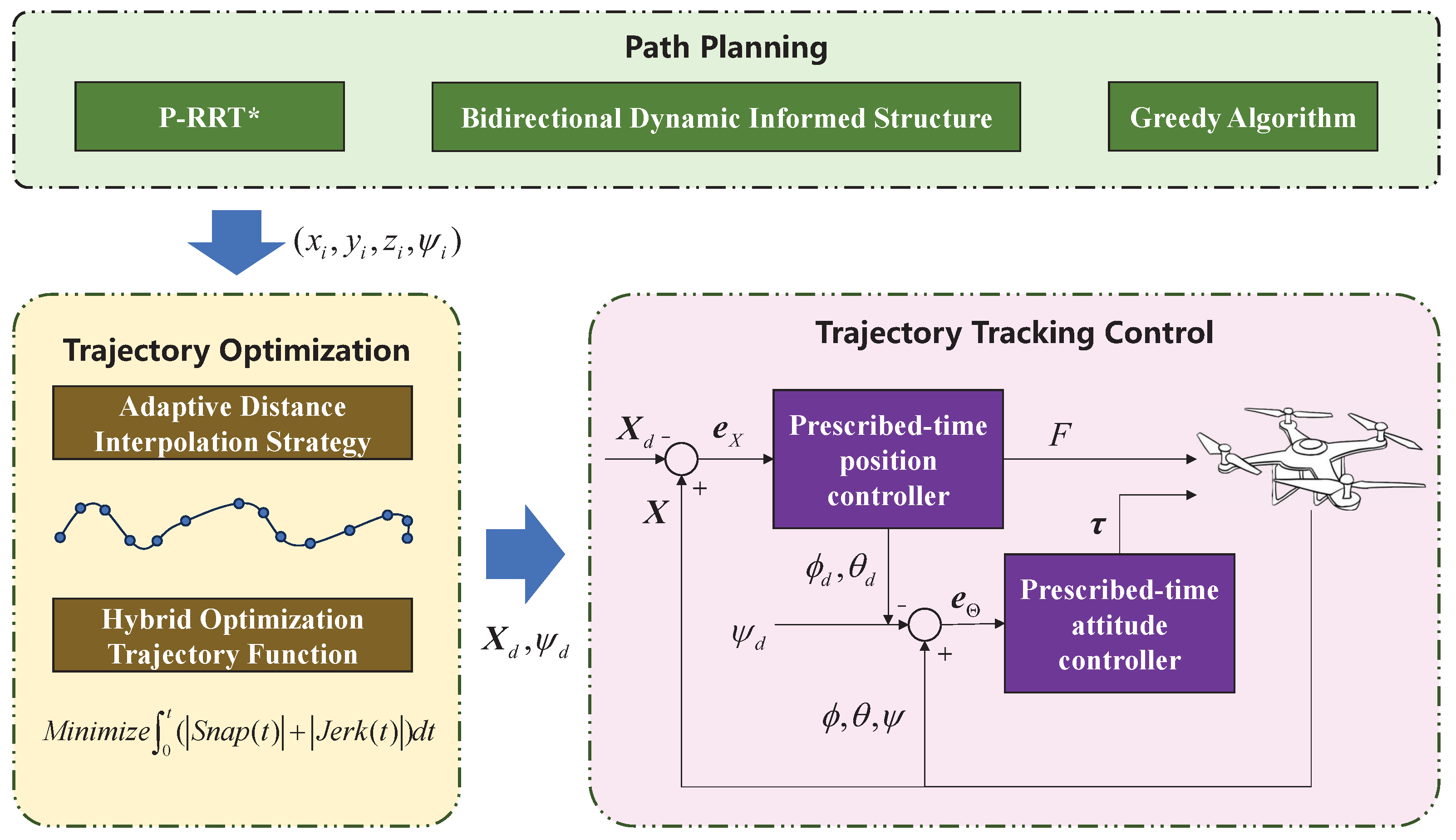
3. Integrated Planning and Control Framework and Algorithm

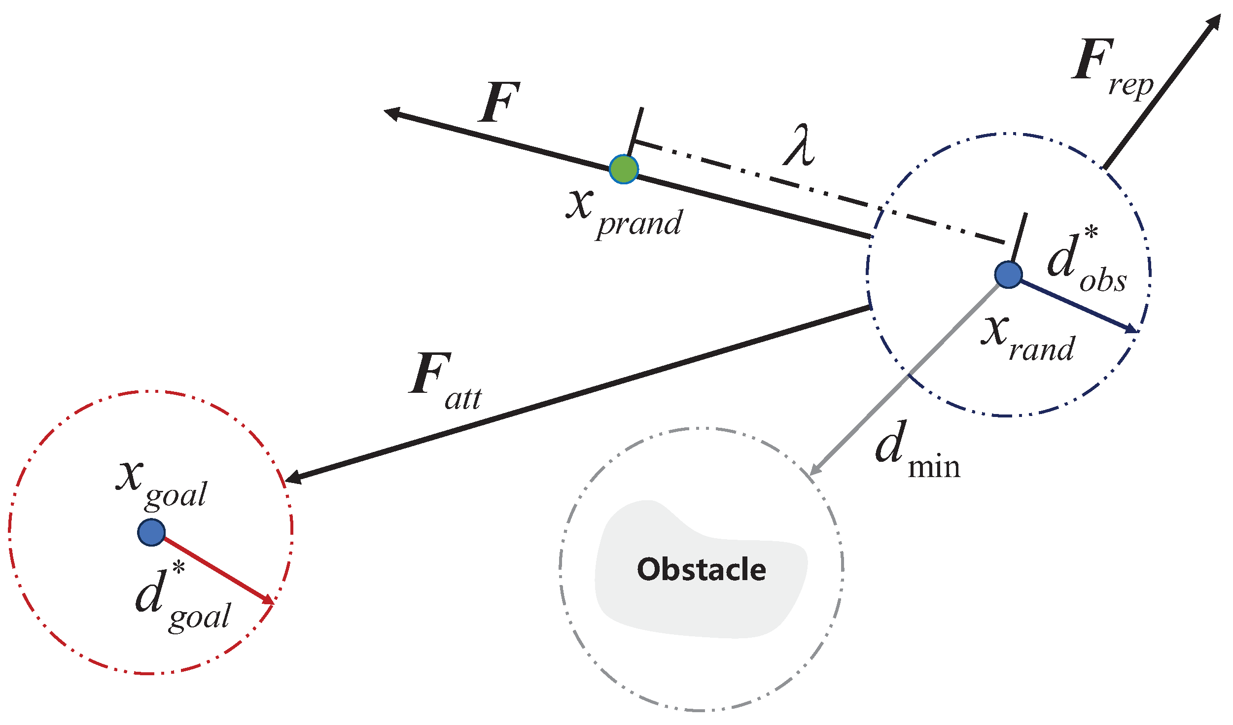
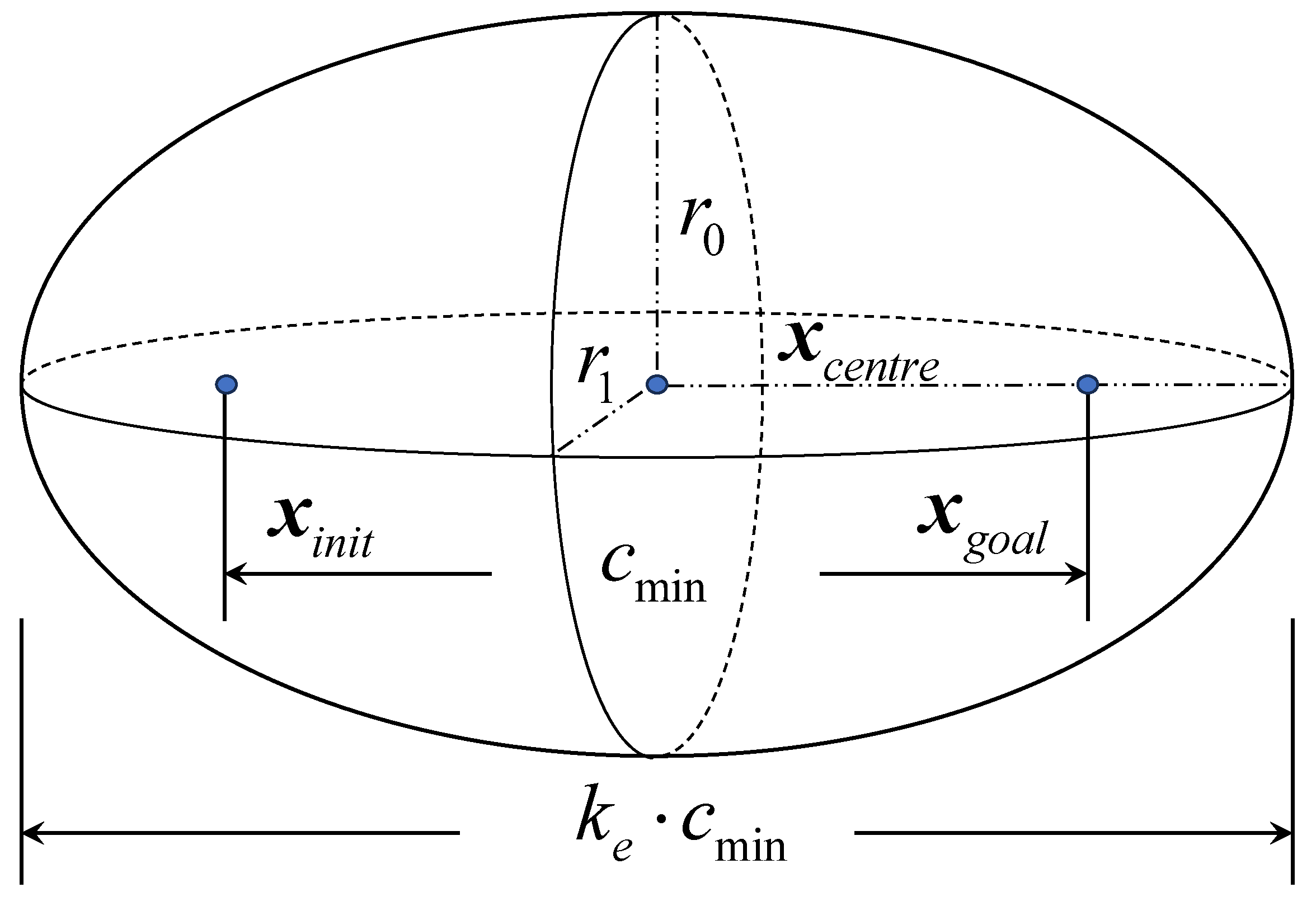
3.1. Advanced Path Planning

To further improve the quality and efficiency of the initial path generation for P-RRT* in scenarios with dense obstacles, a bidirectional dynamic informed structure is implemented to constrain the generation of invalid sampling points and enhance the efficiency of sampling points. Meanwhile, a greedy algorithm is employed to optimize nodes in the proposed BDIP-RRT* by removing redundant nodes and path segments. During the planning process, the safety space or radius between the UAV and obstacles is set to be larger than in typical planning algorithms in order to meet the requirements of trajectory optimization.

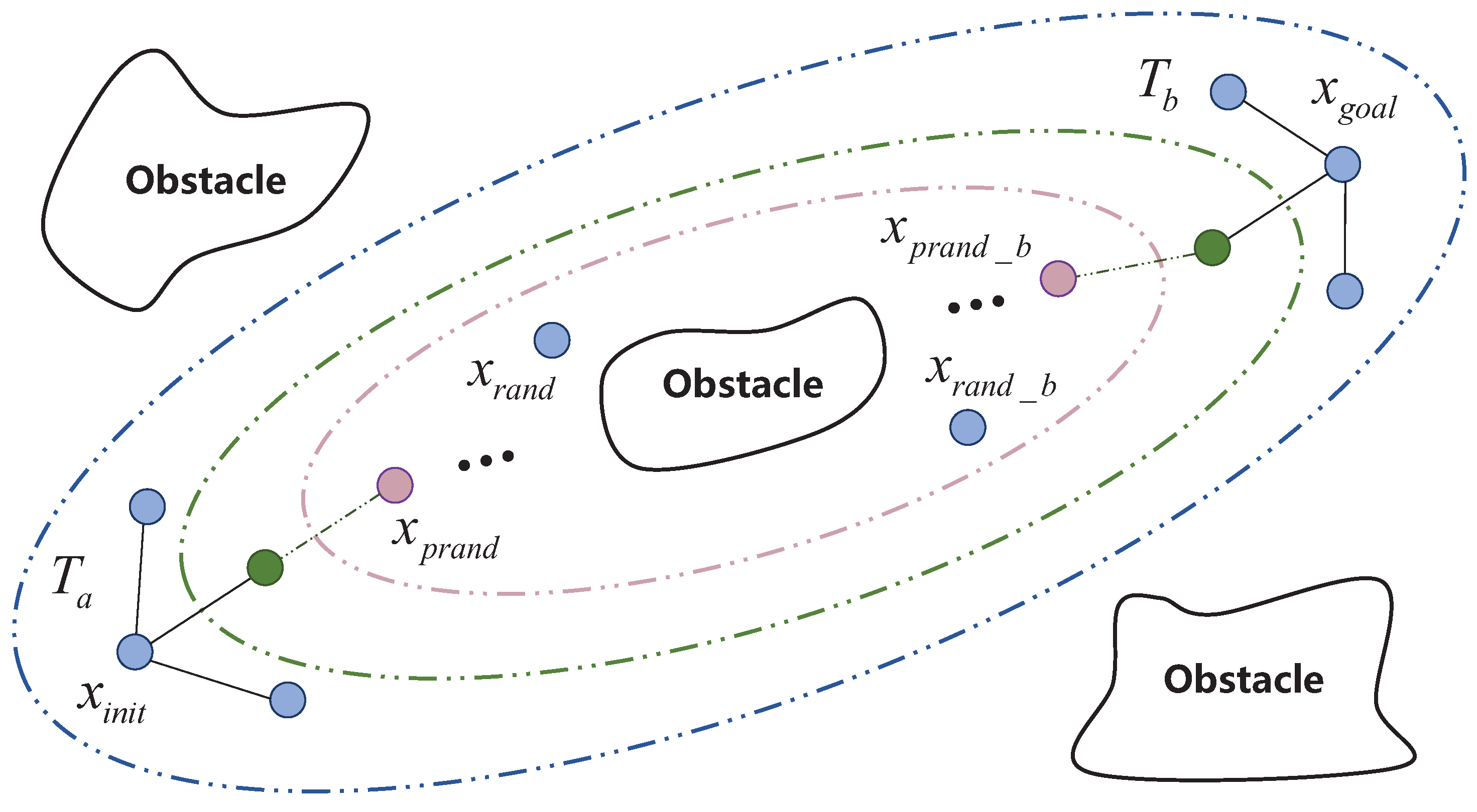
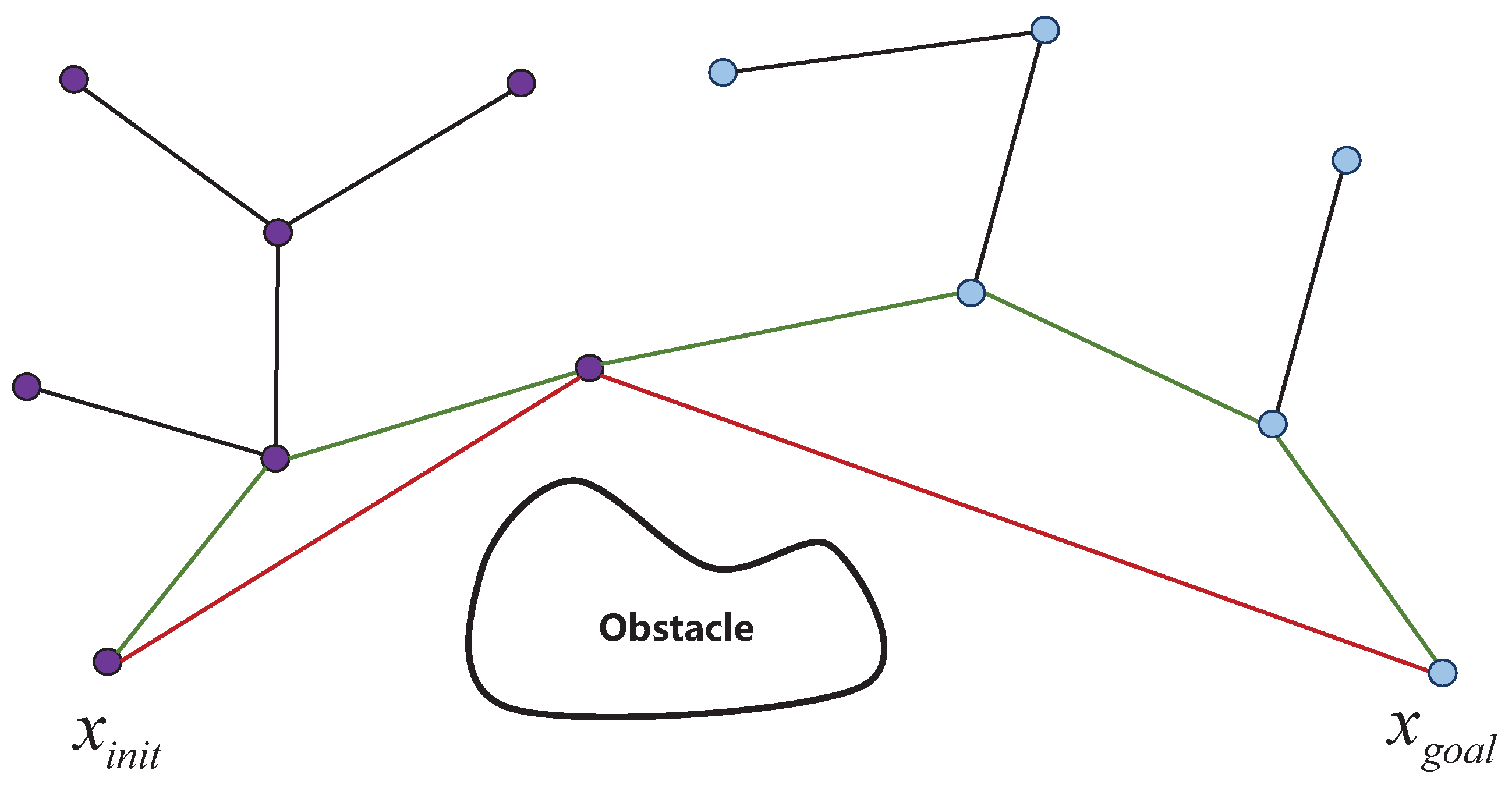
3.1.1. P-RRT* and Bidirectional Dynamic Informed Structure

P-RRT* utilizes the attractive potential field $U_{att}$ and repulsive potential field $U_{rep}$ to generate attractive force ${\mathit{F}}_{att}$ and repulsive force ${\mathit{F}}_{rep}$. This guides the sampling points towards the target while avoiding obstacles, which improves sampling efficiency. The procedure is shown in Figure 2 under the action of the combined force $\mathit{F}$, $x_{prand}=x_{rand}+\lambda ·\mathit{F}/\left|\mathit{F}\right|$, where $\lambda$ is the step size relative to the map size. The algorithm’s flow is detailed in [14].

While P-RRT* enhances sampling point efficiency over RRT*, it lacks adjustments for sampling probability, sampling range, target bias, and multi-tree structure. Moreover, even after potential field guidance a large number of sampling points remain prone to collision with obstacles in dense obstacle scenarios due to the abundance of obstacles and their proximity to the starting point. Increasing the repulsion coefficient may lead to deviation from the endpoint-guided direction, necessitating the introduction of a new structure to enhance its performance. Hence, this paper proposes a novel bidirectional dynamic informed structure inspired by [13,41]. While leveraging the bidirectional multi-tree structure of Bi-RRT*, the proposed structure removes the greedy connectivity approach, opting instead to introduce sample bias through a potential field. Moreover, it incorporates the concept of hyperellipsoid sampling region from Informed RRT* to define the initial sampling region based on the start and end points, as illustrated in Figure 3. Here, $r_0=r_1=\sqrt{{k_e}^2-1}·c_{min}/2$ and $k_e\ge 1$, with the exact value determined by the size of the map and the distribution of obstacles.

The original hyperellipsoid sampling region is constructed in a similar way to [13]. The sampling of a subset of ellipsoids $x_f$ can be expressed as follows:

$$x_f=CL{x}_{ball}+x_{centre}$$

(5)

where C and L are the rotation and transformation matrices, respectively, and $x_{centre}=(x_{init}+x_{goal})/2$ is the midpoint of $x_{init}$ and $x_{goal}$. However, uniform sampling within the hyperellipsoidal region often results in a significant concentration of samples around the center of the hyperellipsoid. In cluttered environments, whether guided by potential fields or raw costs, this leads to numerous collisions between generated trees and obstacles. Frequent collision detection function calls increase the computational burden, reducing sampling efficiency. Therefore, it is necessary to adjust the sampling probability to reduce randomness. A subset of uniformly distributed samples on the surface of an n-ball is selected, denoted as $x_{ballsurf}\sim U\left(X_{ballsurf}\right)$, where $X_{ballsurf}=\{x\in X\mid p^2\le {\left|\right|x\left|\right|}_2\le 1\}$ with $0.5<p<1$. Subsequently, these samples are rotationally transformed, brought into Equation (5) to replace $x_{ball}$, and solved to obtain $x_{fsurf}$. The probabilistic adjustment also needs to be integrated with the bidirectional informed framework. The specific structure is illustrated in Figure 4. The starting point $x_{init}$ and ending point $x_{goal}$ serve as the initial states of the forward tree $T_a$ and reverse tree $T_b$, respectively. During bidirectional exploration, if trees $T_a$ and $T_b$ each contain only a starting or an ending point, then a hyperellipsoidal sampling region is established using these points. However, when trees $T_a$ and $T_b$ each have more than two nodes (including the starting or ending points), then the hyperellipsoidal sampling region is constructed around the parent node of the most recently added node in each spanning tree. This process not only significantly enhances sampling efficiency but also improves the dynamic adaptability of the randomly explored tree, enabling faster generation of high-quality paths with reduced computational redundancy.

Under the bidirectional dynamic informed structure, the two spanning trees undergo continuous dynamic updates until the distance between them is less than a certain threshold. At this point, each spanning tree can be individually backtracked to obtain a path, then the paths from the two spanning trees can be merged into one complete path. This approach fully integrates the four improvement strategies and P-RRT*, significantly improving exploration speed and efficiency in dense obstacle environments.

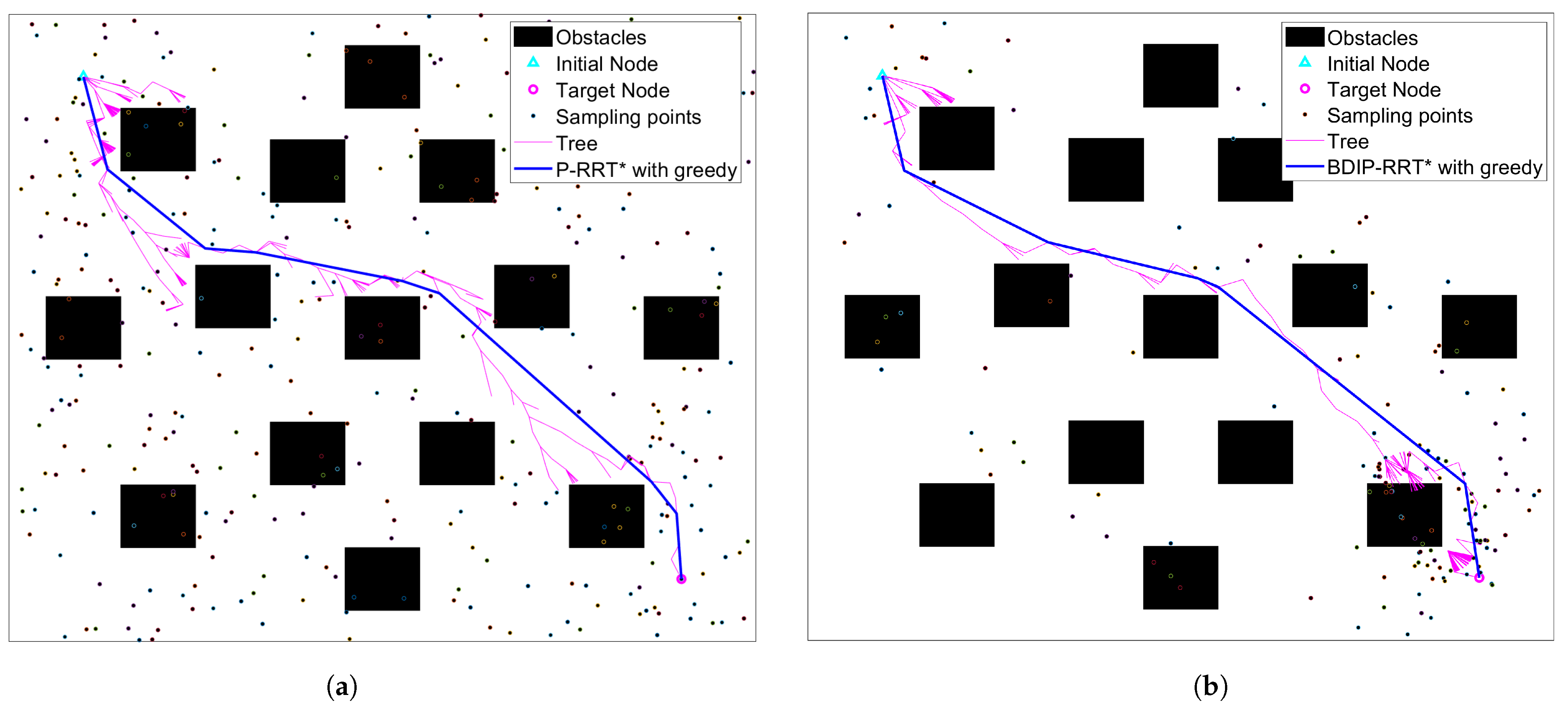
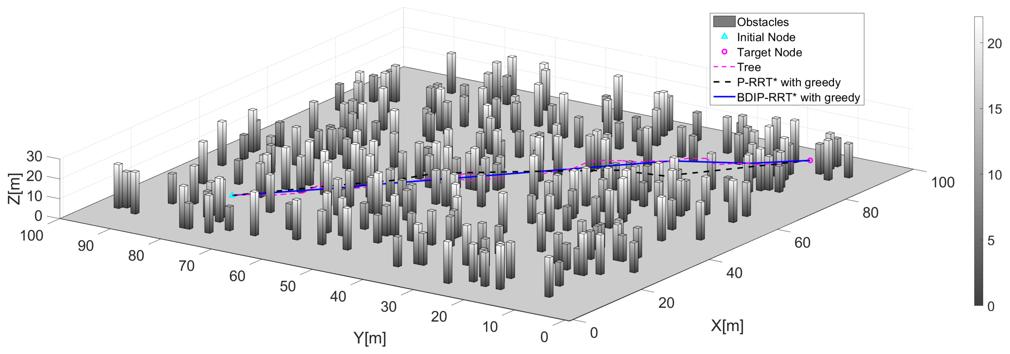
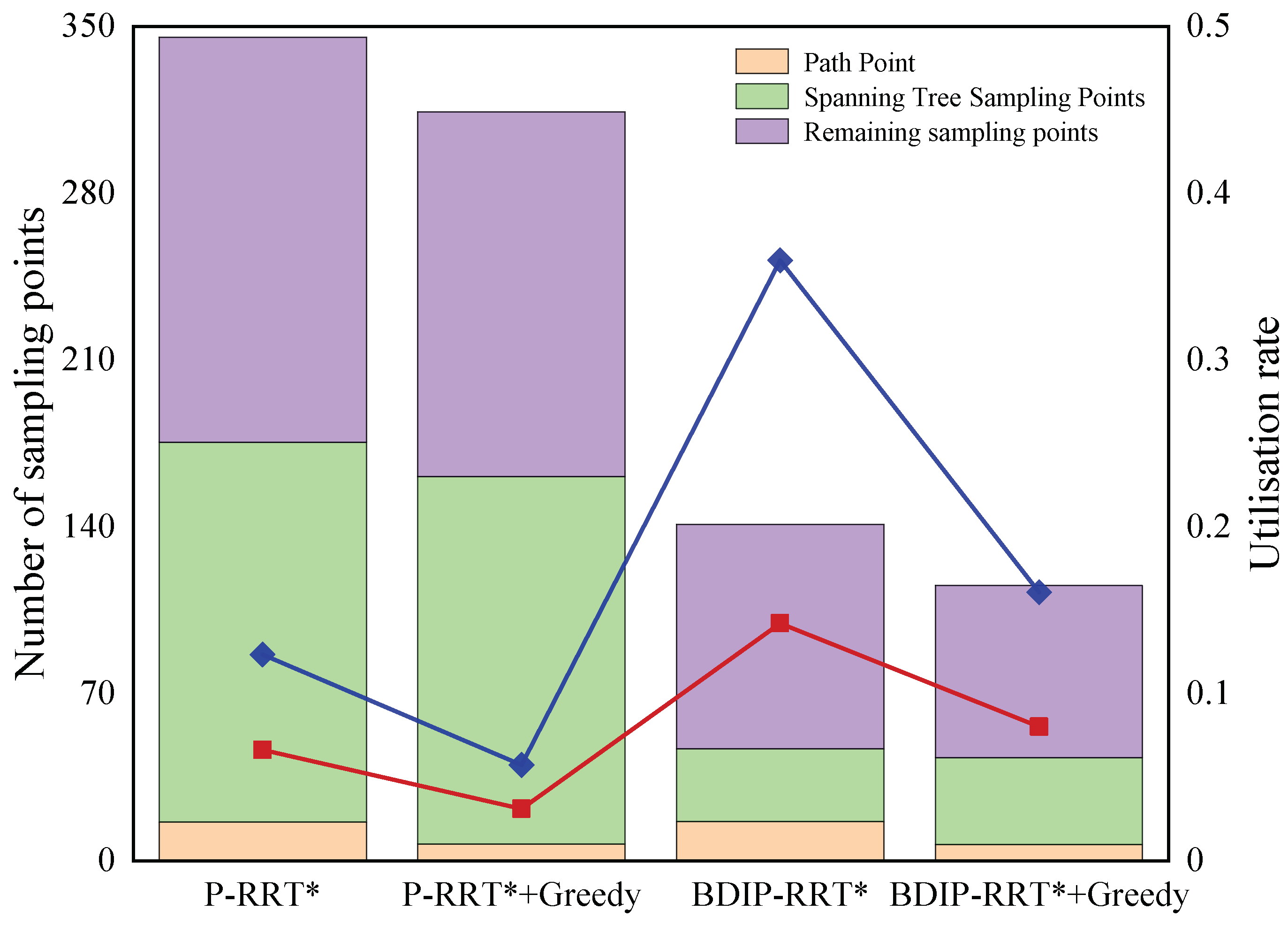
3.1.2. BDIP-RRT* with Greedy Algorithm

In sampling-based algorithms, the paths often include numerous redundant nodes and path segments due to inherent randomness and complex environments. This increases path length and reduces path smoothness, posing challenges for UAV trajectory generation and trajectory tracking control. To address this problem, a greedy algorithm is adopted to improve the smoothness and quality of the generated path. Figure 5 shows the basic principle of the greedy algorithm, in which purple dots represent nodes on $T_a$, blue dots are nodes on $T_b$, and black line segments indicate the parts of the two spanning trees. The green line segment represents the overall path obtained by backtracking the two spanning trees, while the red illustrates the improved path generated by the greedy algorithm. This algorithm connects the starting point of the global path to all other path points except the second point, then conducts collision detection. If there is no collision, then the intermediate path points are simply omitted. These steps are repeated from the second node of the latest generated path, continuously updating the path until reaching the endpoint.

P-RRT* improves sampling point quality by integrating a potential field function into the RRT* framework. It further enhances the multi-tree structure, sampling range, target bias, and probability selection through the introduction of a bidirectional dynamic informed approach. The performance comparison between P-RRT* and BDIP-RRT* combined with the greedy algorithm on a 2D map shows the results at the point of initial discovery of connected paths, as illustrated in Figure 6.

Notably, the BDIP-RRT* algorithm proposed in this work exhibits substantially fewer sampling nodes compared to P-RRT*, resulting in significantly fewer spanning trees. Moreover, the number of collisions in the dead zone is dramatically reduced, enhancing sampling efficiency and enabling expedited discovery of the final path.

Table 1. Comparison of algorithm combinations in 2D map.

Algorithms	Length (m)	Time (s)
P-RRT*	25.385	0.925
P-RRT* with greedy	24.773	0.631
BDIP-RRT*	24.943	0.410
BDIP-RRT* with greedy	24.588	0.308

compares the costs and computation times of different combinations of algorithms, revealing a 1.31% decrease in path length and a 51.19% reduction in computation time. These results demonstrate the superior effectiveness of the proposed BDIP-RRT* with greedy over P-RRT* in dense obstacle environments. The specific algorithmic procedure is depicted in Algorithm 1. Finally, BDIP-RRT* with the greedy algorithm generates a series of discrete path points $p{p}_i=(x_i,y_i,z_i)$ in three-dimensional space, where $i=1,2,\cdots ,N$. These path points can be represented as $PP=\{p{p}_1,p{p}_2,\cdots ,p{p}_N\}$, where N represents the total number of elements in the collision-free path point set.

Algorithm 1 BDIP-RRT* with greedy ($x_{init}$, $x_{goal}$)

1: $V_a\leftarrow \left\{x_{init}\right\}$; $V_b\leftarrow \left\{x_{goal}\right\}$; 2: $E_a\leftarrow ⌀$; $E_b\leftarrow ⌀$; 3: $T_a\leftarrow (V_a,E_a)$; $T_b\leftarrow (V_b,E_b)$; 4: for  $n\leftarrow 0$ to  N  do 5:    if $x_{new}$ exists and $x_{newb}$ exists then 6:        $x_{rand}$ = Ellipse($x_{new\_parent}$, $x_{newb\_parent}$); 7:    else 8:      $x_{rand}$ = Ellipse($x_{init}$, $x_{goal}$); 9:    end if 10:  $x_{prand}\leftarrow$ RGD($x_{rand}$); 11:  $x_{nearest}\leftarrow$ NearestNode($x_{prand}$, $T_a$); 12:  $x_{new}\leftarrow$ Steer ($x_{nearest}$, $x_{prand}$); 13:  $X_{near}\leftarrow$ NearbyNodes($x_{new}$, $T_a$); 14:  $L\leftarrow$ ListSort($x_{new}$, $X_{near}$); 15:  $x_{parent}\leftarrow$ ChooseBestParent(L); 16:  if $x_{parent}$ exists then 17:      $T_a\leftarrow$ InsertNode($x_{new}$, $x_{parent}$, $T_a$); 18:      $E_a\leftarrow$ Rewire($x_{new}$, L, $E_a$); 19:      $x_{nearestb}\leftarrow$ NearestNode($x_{new}$, $T_b$); 20:      $x_{randb}\leftarrow$ Ellipse($x_{init}$, $x_{goal}$); 21:      $x_{prandb}\leftarrow$ RGD($x_{randb}$); 22:      $x_{newb}\leftarrow$ Steer ($x_{nearestb}$, $x_{prandb}$); 23:      $X_{nearb}\leftarrow$ NearbyNodes($x_{newb}$, $T_b$); 24:      $L_b\leftarrow$ ListSort($x_{newb}$, $X_{nearb}$); 25:      $x_{parentb}\leftarrow$ ChooseBestParent($L_b$); 26:      if $x_{parentb}$ exists then 27:          $T_b\leftarrow$ InsertNode($x_{newb}$, $x_{parentb}$, $T_b$); 28:          $E_b\leftarrow$ Rewire($x_{newb}$, $L_b$, $E_b$); 29:          if collisionFree($x_{new}$,$x_{newb}$) then 30:              path = GreedyOpt(ExtPath($T_a$,$T_b$)); 31:              return path; 32:         end if 33:      end if 34:    end if 35: end for

3.2. Comprehensive Trajectory Optimization

The path points generated by path planning constitute a sequence of position vectors from the starting point to the target point without including time information. However, trajectory tracking control necessitates a continuous trajectory that is high-order differentiable with respect to time, including the flight states of the UAV. Hence, in this subsection we develop a new three-dimensional optimized trajectory generator utilizing polynomial functions concerning time. Trajectory control points are selected based on an adaptive distance interpolation strategy, while a hybrid optimized function calculates polynomial coefficients to generate a continuous trajectory.

3.2.1. Adaptive Distance Interpolation Strategy

In situations with dense obstacles, trajectory quality is vital to the stability and safety of UAVs. Thus, selecting appropriate trajectory control points is crucial to avoid sudden motion changes and improve tracking performance. Using interpolation to reduce collisions is less complex than adding avoidance constraints; however, excessive interpolation can cause trajectory deviations, necessitating a balance between motion state and trajectory accuracy. Due to the larger safety radius set in Section 3.1, allowing some trajectory deviation can improve motion states. To further reduce deviation, an adaptive distance interpolation strategy is employed. First, the yaw angle between each adjacent pair of path points is calculated using

$${\psi }_i=\left\{\begin{array}{cc}arctan{\displaystyle \frac{y_{i+1}-y_i}{x_{i+1}-x_i}}\hfill & i=1,2,\cdots ,N-1,\hfill \\ {\psi }_{N-1}\hfill & i=N,\hfill \end{array}\right.$$

(6)

where ${\psi }_i$ denotes the yaw angle of the ith path point. The yaw angle at the endpoint defaults to the yaw angle of the second-to-last path point. The distance $d_i$ between each pair of neighboring points needs to be calculated, and the total path length D can be expressed as $D={\sum }_{i=1}^{N-1}{d}_i$. During subsequent trajectory point design, $d_i$ is updated as the sequence of trajectory control points changes.

Subsequently, trajectory control points $t{p}_{ib}$ and $t{p}_{if}$ with a fixed minimum distance $d_{fix}$ are generated before and after each path point $p{p}_i$ except for the starting point $p{p}_1$ and ending point $p{p}_N$. The generated sequence of trajectory control points is $TP=\{p{p}_1,t{p}_{2b},t{p}_{2f},\cdots ,t{p}_{ib},t{p}_{if},\cdots ,p{p}_N\}=\{t{p}_1,t{p}_2,\cdots ,t{p}_{2N-2}\}$. This method effectively reduces unreasonable roundabouts caused by angular variations by smoothing the transitions and controlling the path curvature.

Furthermore, it is desirable to obtain the distance by comparing the updated $d_i$ with $se{g}_{min}$ and $se{g}_{max}$. If $d_i\ge se{g}_{min}$, then it stays the same; otherwise, it is replaced with the midpoints of the two endpoints of $d_i$. Updating the sequence of trajectory control points in this way prevents sharp oscillations in the trajectory caused by excessive interpolation points. If $d_i\le se{g}_{max}$, then no modifications are made; otherwise $se{g}_{num}$ is calculated in the following form:

$$se{g}_{num}=⌈{\displaystyle \frac{d_i}{se{g}_{max}}}⌉$$

(7)

where $⌈·⌉$ indicates the operation of rounding up. The distance between neighboring trajectory points is divided into $se{g}_{num}$ segments, with $se{g}_{num}-1$ intermediate points added, except near the starting and ending points for flight stability. This update to the trajectory control point sequence prevents trajectory divergence and ensures accuracy. Here, the values of $se{g}_{min}$ and $se{g}_{max}$ depend on $d_i$ and the total path D. As the connections between path points are straight lines, the yaw angle of the inserted point is the same as the yaw angle of the nearest initial path point in the direction of the starting point.

3.2.2. Hybrid Optimization Trajectory Function

In light of the UAV’s dynamics and differential flatness characteristics, it can be understood that the third-order derivatives of trajectory polynomials correspond to the UAV’s jerk and angular velocity [42]. Similarly, the fourth-order derivatives correspond to snap and angular acceleration, with the latter influencing energy consumption [43]. Given the need to minimize energy consumption and angular velocity variations during obstacle avoidance in dense environments, a new hybrid optimized trajectory objective function is devised in this subsection, aiming to minimize both jerk and snap.

The complex spatial trajectory is represented using a combination of multiple trajectory segments, with each segment described by an nth-order polynomial function. The entire trajectory is expressed as

$$p\left(t\right)=\left\{\begin{array}{cc}\sum _{j=0}^n{p}_{1,j}{t}^j,\hfill & t_0\le t<t_1\hfill \\ \sum _{j=0}^n{p}_{2,j}{t}^j,\hfill & t_1\le t<t_2\hfill \\ ⋮\hfill \\ \sum _{j=0}^n{p}_{N-1,j}{t}^j,\hfill & t_{N-2}\le t<t_{N-1}.\hfill \end{array}\right.$$

(8)

The hybrid optimized trajectory function is designed in the following form:

$$minf\left(p\right)=min{\lambda }_1{f}_{snap}\left(p\right)+{\lambda }_2{f}_{jerk}\left(p\right)$$

(9)

where ${\lambda }_1$ and ${\lambda }_2$ are the weighting factors and where $f_{snap}$ and $f_{jerk}$ are calculated as follows:

$$f_{snap}\left(p\right)={\int }_0^T{\left(p^{\left(4\right)}\left(t\right)\right)}^{2}dt,$$

(10)

$$f_{jerk}\left(p\right)={\int }_0^T{\left(p^{\left(3\right)}\left(t\right)\right)}^{2}dt.$$

(11)

Equation (10) can be converted to the following form:

$$\begin{array}{cc}\hfill f_{snap}\left(p\right)& =\sum _{i=1}^{N-1}{\int }_{t_{i-1}}^{t_i}{\left(p^{\left(4\right)}\left(t\right)\right)}^2\mathrm{d}t\hfill \\ \hfill & =\sum _{i=1}^{N-1}{p}^T{\int }_{t_{i-1}}^{t_i}{[0,0,0,0,24,\dots ,{\displaystyle \frac{n!}{(n-4)!}}{t}^{n-4}]}^T\hfill \\ \hfill & \phantom{=}[0,0,0,0,24,\dots ,{\displaystyle \frac{n!}{(n-4)!}}{t}^{n-4}]dt p\hfill \\ \hfill & =\sum _{i=1}^{N-1}{p}^T{Q}_{sna{p}_i}p=p^T{Q}_{snap}p\hfill \end{array}$$

(12)

with

$$Q_{sna{p}_i}=\left[\begin{array}{cc}{0}_{4\times 4}& 0_{4\times (n-3)}\\ 0_{(n-3)\times 4}& {\displaystyle \frac{l!q!(t_i^{(l+q-7)}-t_{i-1}^{(l+q-7)})}{(l-4)!(q-4)!(l+q-7)}}\end{array}\right]$$

(13)

$$Q_{snap}=\left[\begin{array}{cccc}{Q}_{sna{p}_1}& & & \\ & Q_{sna{p}_2}& & \\ & & \ddots & \\ & & & Q_{sna{p}_{N-1}}\end{array}\right].$$

(14)

Then, we can obtain

$$f_{jerk}\left(p\right)=p^T{Q}_{jerk}p$$

(15)

$$Q_{jer{k}_i}=\left[\begin{array}{cc}{0}_{3\times 3}& 0_{3\times (n-2)}\\ 0_{(n-2)\times 3}& {\displaystyle \frac{l!q!(t_i^{(l+q-5)}-t_{i-1}^{(l+q-5)})}{(l-3)!(q-3)!(l+q-5)}}\end{array}\right]$$

(16)

$$Q_{jerk}=\left[\begin{array}{cccc}{Q}_{jer{k}_1}& & & \\ & Q_{jer{k}_2}& & \\ & & \ddots & \\ & & & Q_{jer{k}_{N-1}}\end{array}\right],$$

(17)

where l and q are the row index and column index of a matrix, with indexing starting from 0.

Hence, the UAV’s trajectory optimization can be reformulated as a quadratic programming problem. The objective function for the hybrid optimized trajectory is depicted in the following form:

$$minf\left(p\right)=min{p}^T({\lambda }_1{Q}_{snap}+{\lambda }_2{Q}_{jerk})p.$$

(18)

It is worth mentioning that generation of the hybrid optimized trajectory involves two main motion constraints, namely, endpoint state constraints (initial, final, and intermediate states) and continuity constraints, ensuring equal higher-order derivatives between adjacent trajectories. The polynomial coefficients p are solved using the method in [21], and substituting p into (8) provides the desired trajectory ${\mathit{X}}_d$ and yaw angle ${\psi }_d$.

3.3. Prescribed-Time Trajectory Tracking Control

To meet the requirements of fast response and strong robustness for the UAV in scenarios with dense obstacles, two novel prescribed-time position and attitude control laws are designed to ensure rapid and precise trajectory tracking performances. The desired trajectory ${\mathit{X}}_d={[x_d,y_d,z_d]}^{\mathrm{T}}$ and desired yaw angle ${\psi }_d$ can be derived from Section 3.2. Through an analysis of the UAV’s underdrive characteristics, it becomes evident that ${\varphi }_d$ and ${\theta }_d$ can be determined by ${\mathit{X}}_d$ and ${\psi }_d$ [44]. The corresponding calculations are as follows:

$${\varphi }_d=arcsin\left({\displaystyle \frac{u_{a1}sin{\psi }_d-u_{a2}cos{\psi }_d}{\left|\right|{\mathit{u}}_a\left|\right|}}\right),$$

(19)

$${\theta }_d=arctan\left({\displaystyle \frac{u_{a1}cos{\psi }_d+u_{a2}sin{\psi }_d}{u_{a3}}}\right),$$

(20)

with ${\mathit{u}}_a={[u_{a1},u_{a2},u_{a3}]}^{\mathrm{T}}=\mathit{u}/m$. The desired attitude is defined as ${\mathbf{\Theta }}_d={[{\varphi }_d,{\theta }_d,{\psi }_d]}^{\mathrm{T}}$. Then, the tracking errors are defined as ${\mathit{X}}_e=\mathit{X}-{\mathit{X}}_d$ and ${\mathbf{\Theta }}_e=\mathbf{\Theta }-{\mathbf{\Theta }}_d$. We define ${\mathit{x}}_{p1}={\mathit{X}}_e$, ${\mathit{x}}_{p2}={\dot{\mathit{X}}}_e$, ${\mathit{x}}_{a1}={\mathbf{\Theta }}_e$ and ${\mathit{x}}_{a2}={\dot{\mathbf{\Theta }}}_e$. Let ${\mathit{f}}_p=-g{\mathit{z}}_I-{\ddot{\mathit{X}}}_d$ and ${\mathit{f}}_a=-{\mathit{J}}^{-1}\mathit{C}\dot{\mathbf{\Theta }}-{\ddot{\mathbf{\Theta }}}_d$. Then, Equations (1) and (2) can be rewritten in the following form:

$$\left\{\begin{array}{c}{\dot{\mathit{x}}}_{p1}={\mathit{x}}_{p2}\hfill \\ {\dot{\mathit{x}}}_{p2}={\displaystyle \frac{1}{m}}\mathit{u}+{\mathit{f}}_p\hfill \end{array}\right.$$

(21)

$$\left\{\begin{array}{c}{\dot{\mathit{x}}}_{a1}={\mathit{x}}_{a2}\hfill \\ {\dot{\mathit{x}}}_{a2}={\mathit{J}}^{-1}\mathit{\tau }+{\mathit{f}}_a.\hfill \end{array}\right.$$

(22)

Lemma 1

([39]). Consider the normal-form system described by ${\dot{x}}_i=x_{i+1}$ for $i=1,\cdots ,n-1$ and ${\dot{x}}_n=f(x,t)+b(x,t)u$, where $x=[x_1,\cdots ,x_n]$ and where $u\in \mathbb{R}$ is the control input. The functions $f(x,t)$ and $b(x,t)$ are smooth, bounded, and non-vanishing. We introducing a time scale function $\mu (t-t_0)={\mu }_1{(t-t_0)}^{h+n}={(T/(T+t_0-t))}^{h+n}$ on $t\in [t_0,t_0+T)$, where h is a positive integer and T is the prescribed settling time. If the prescribed-time control law is designed as $u=-(f+L_0+L_1+kz)/b$, in which $k>0$ and the definitions of $L_0$, $L_1$, and z are provided in [39], then there exist constants $\tilde{M},\tilde{\delta }>0$ such that $\left|x\left(t\right)\right|\le \nu {(t-t_0)}^{h+1}\tilde{M}{\mathrm{e}}^{-\tilde{\delta }(t-t_0)}\left|x\left(t_0\right)\right|$ with $\nu (t-t_0)={\mu }_1{(t-t_0)}^{-1}$.

In the second-order system provided by (21), the control law is formulated using auxiliary variables $\mathit{\omega }=\kappa {\mathit{x}}_p$ and $\mathit{z}=\dot{\mathit{\omega }}+{\rho }_{1p}\mathit{\omega }$, where ${\mathit{x}}_p={[{\mathit{x}}_{p1},{\mathit{x}}_{p2}]}^{\mathrm{T}}$, $\kappa ={\left({\mu }_1{\chi }_1\right)}^{h+2}$, and ${\rho }_{1p}>0$. The functions ${\mu }_1$ and ${\chi }_1$ are defined as

$${\mu }_1(t-t_0)=\left\{\begin{array}{cc}{\displaystyle \frac{T}{T+t_0-t}},\hfill & t\in [t_0,t_0+T)\hfill \\ C\hfill & t\in [t_0+T,\infty ),\hfill \end{array}\right.$$

(23)

where C is a constant and

$${\chi }_1(t-t_0)=\left\{\begin{array}{cc}1-tan\left({\displaystyle \frac{\pi }{4}}·{\displaystyle \frac{t-t_0-t_1}{T-t_1}}\right),\hfill & t\in [t_0+t_1,t_0+T)\hfill \\ 1\hfill & \mathrm{otherwise},\hfill \end{array}\right.$$

(24)

with $0<t_1<T$. Consequently, the control input is provided by

$$\mathit{u}=m(g{\mathit{z}}_I+{\ddot{\mathit{X}}}_d-({\mathit{ϵ}}_1+{\mathit{ϵ}}_2)-{\rho }_1\mathit{z}),$$

(25)

where ${\mathit{ϵ}}_1=2\dot{\kappa }{\mathit{x}}_{p2}/\kappa +\ddot{\kappa }{\mathit{x}}_{p1}/\kappa$ and ${\mathit{ϵ}}_2={\rho }_{1p}\dot{\kappa }{\mathit{x}}_{p1}/\kappa +{\rho }_{1p}{\mathit{x}}_{p2}$, ${\rho }_1>0$.

Remark 1.

In Lemma 1, when μ goes to infinity and $\mathit{x}$ goes to zero, $\mu \mathit{x}$ is bounded ideally; however, $\mathit{x}$ may not fully decay to zero while the gain μ continues to grow unbounded, potentially leading to a singularity-like issue. Therefore, the controller design employs piecewise functions with a tangent component to restrict the excessive growth of the scaling function when it becomes sufficiently large with $t\in [t_0,t_0+T)$. Thus, when $t\ge t_0+T$, μ becomes a constant C.

Theorem 1.

Consider the UAV position error system in (21). If the prescribed-time control law is designed as $\mathit{u}$, that is, developed as in (25), then the UAV can rapidly achieve precise trajectory tracking within the predefined time T.

Proof of Theorem 1. 

Consider the Lyapunov function candidate $V={\mathit{z}}^{\mathrm{T}}\mathit{z}/2$. The derivative of V can be expressed as follows:

$$\begin{array}{cc}\hfill \dot{V}& =\kappa {\mathit{z}}^{\mathrm{T}}({\displaystyle \frac{1}{m}}\mathit{u}+{\mathit{f}}_p+({\mathit{ϵ}}_1+{\mathit{ϵ}}_2)),\hfill \\ \hfill & ={\chi }_1^{h+2}\mu {\mathit{z}}^{\mathrm{T}}({\displaystyle \frac{1}{m}}\mathit{u}+{\mathit{f}}_p+({\mathit{ϵ}}_1+{\mathit{ϵ}}_2)),\hfill \\ \hfill & \le \mu {\mathit{z}}^{\mathrm{T}}({\displaystyle \frac{1}{m}}\mathit{u}+{\mathit{f}}_p+({\mathit{ϵ}}_1+{\mathit{ϵ}}_2)).\hfill \end{array}$$

(26)

Upon applying the control law in (25), $\dot{V}\le -2{\rho }_1\mu V$ can be derived from (26), yielding

$$\left|\right|\mathit{z}\left(t\right)\left|\right|\le \zeta {(t-t_0)}^{{\rho }_1}\left|\right|\mathit{z}\left(t_0\right)\left|\right|,$$

(27)

with $\zeta (t-t_0)={exp}^{{\displaystyle \frac{T}{h+1}}(1-{\mu }_1{(t-t_0)}^{h+1})}$. Based on the cascade relationship between $\mathit{z}$, $\mathit{w}$, and $\mathit{x}$ provided by

$$\mathit{z}=\mu {\left[\begin{array}{c}{\displaystyle \frac{h+2}{T}}{\mu }_1+{\rho }_1\\ 1\end{array}\right]}^{\mathrm{T}}{\mathit{x}}_p=\mu \mathit{A}{\mathit{x}}_p,$$

(28)

we can further obtained

$$\left|\right|{\mathit{x}}_p\left|\right|\le {\nu }^{h+2}{\left|\right|\mathit{A}\left|\right|}^{-1}\zeta {(t-t_0)}^{{\rho }_1}\left|\right|A\left(t_0\right){\mathit{x}}_p\left(t_0\right)\left|\right|.$$

(29)

Because $\nu$ and $\zeta {(t-t_0)}^{{\rho }_1}$ goes to zero as $t\to t_0+T$, $\left|\right|{\mathit{x}}_p\left|\right|$ goes to zero as $t\to t_0+T$. Thus, the proof is complete. □

Similarly, the attitude control law for the system in (22) can be designed as follows:

$$\mathit{\tau }=\mathit{J}({\mathit{J}}^{-1}\mathit{C}\dot{\mathbf{\Theta }}+{\ddot{\mathbf{\Theta }}}_d-({\mathit{ϵ}}_1+{\mathit{ϵ}}_2)-{\rho }_2\mathit{z}).$$

(30)

The proof is similar to the last proof, and is consequently omitted.

4. Numerical Simulation

To validate the integrated design encompassing path planning, optimized trajectory generation, and trajectory tracking control for a UAV within densely cluttered obstacle environments, a three-dimensional environment measuring 100 × 100 × 30 units with 250 cylindrical obstacles was established in MATLAB/Simulink. Given the inherently stochastic nature of RRT algorithms in both P-RRT* [14] and BDIP-RRT*, a single dataset is insufficient to accurately demonstrate the overall superiority of BDIP-RRT* over P-RRT*. To demonstrate the advantages of BDIP-RRT*, 50 independent experimental trials were conducted in a Matlab-based 3D dense obstacle environment, with the generated datasets analyzed through statistical distribution methods for comparative performance evaluation.

The best-performing results among the 50 sets of data were selected for both algorithms (P-RRT* with greedy and BDIP-RRT* with greedy), as shown in Figure 7. Considering the safety performance of quadrotor UAVs, the minimum safety distance was set to 0.5 m during the planning process. The step size was set to 3 m to ensure both fast convergence and adequate resolution in dense obstacle environments. If a sampled point did not directly collide with an obstacle but the shortest distance between them was less than the sum of the minimum safe distance and the UAV’s radius, the point was regarded as a collision risk and was excluded. We observed that P-RRT* with greedy is susceptible to the influence of potential fields, often resulting in suboptimal paths excessively avoiding obstacles. BDIP-RRT* with greedy partially mitigates this issue, demonstrating higher planning efficiency. The specific data are presented in

Table 2. Comparison of algorithm combinations in 3D map.

Algorithms	Length (m)	Time (s)
P-RRT* with greedy	99.296	0.133
BDIP-RRT* with greedy	96.596	0.049

, indicating that BDIP-RRT* with greedy reduces the path length by 2.72% compared to P-RRT* with greedy, with a corresponding 63.16% reduction in time.

As shown in Figure 8, we conducted a comparative analysis of the path length and generation time metrics for the different algorithms and their combinations. Figure 8a indicates that both the P-RRT* and BDIP-RRT* algorithms are more effectively in reducing the path length and less susceptible to outliers when combined with the greedy algorithm. Notably, BDIP-RRT* combined with the greedy algorithm results in the shortest path length. Figure 8b demonstrates that BDIP-RRT* and BDIP-RRT* with greedy are both significantly faster in terms of path generation compared to P-RRT* and P-RRT* with greedy, highlighting the superiority of BDIP-RRT* in terms of generation speed. As further illustrated in

Table 3. Mean and standard deviation of path length and path planning time for BDIP-RRT* with greedy algorithm (50 trials).

Algorithm	Metrics	Length (m)	Time (s)
P-RRT* with greedy	Mean	101.696	0.575
	Standard deviation	3.256	0.393
BDIP-RRT* with greedy	Mean	98.202	0.124
	Standard deviation	1.370	0.063

, BDIP-RRT* with greedy also outperforms P-RRT* with greedy in terms of mean and standard deviation for both path length and generation time. Considering both path length and generation time, BDIP-RRT* with greedy demonstrates the best overall performance among the tested algorithms.

Because the efficiency of the RRT algorithm during path generation fundamentally depends on the quality of the sampling points, we compared the number of total sampling points, spanning tree sampling points, and path points in order to provide a more intuitive comparison between algorithm combinations. As shown in Figure 9, the number of total sampling points for BDIP-RRT* and its combination with the greedy algorithm are significantly smaller than for P-RRT* and its combination with the greedy algorithm. The role of the greedy algorithm is mainly to remove redundant nodes in the path; thus, the total sampling points and spanning tree sampling points are primarily determined by the BDIP-RRT* algorithm. The blue line represents the ratio of path points to total sampling points, while the red line represents the ratio of path points to spanning tree sampling points. The utilization trends of both ratios are essentially the same, demonstrating the stability of the algorithms. Because the greedy algorithm eliminates redundant nodes along the path, the utilization rates of the combined algorithms are lower than those of the standalone algorithms.

Control point selection and time allocation are conducted after obtaining the series of discrete path points through path planning, which directly affects the trajectory generation performance. During UAV operations, the average velocity was fixed at 2 m/s while adhering to $d_{fix}=4\mathrm{m}$, $se{g}_{min}=6\mathrm{m}$ and $se{g}_{max}=12\mathrm{m}$. In Figure 10, the blue dots represent trajectory control points, while the red segments depict the generated 3D trajectory. It is evident that the generated trajectory exhibits smooth transitions without any abrupt changes. Compared to the originally generated path in 3D space in Figure 11, it can be observed that the generated trajectory closely aligns with the initial path in most regions. To ensure control performance, the generated trajectory deviates from the initial path in certain areas; however, due to the implementation of a substantial safety margin during the planning process, these deviations do not result in collisions with obstacles.

To further demonstrate the smoothness and continuity of the trajectory, a higher-order derivative analysis of the 3D trajectory was performed, with the results illustrated in Figure 12. The results shows that the changes in the higher-order derivatives of the trajectory do not exhibit any significant abrupt transitions. Due to the need to satisfy position, velocity, and acceleration constraints at the starting and ending points, the oscillations are more pronounced in these regions compared to the middle portion of the trajectory. Nevertheless, the overall trajectory maintains a high degree of smoothness. Except for the velocity derivative (first-order derivative), which shows more noticeable variations with the trajectory changes, the other higher-order derivatives all remain within the range of −1 to 1. These stable trajectory parameters provide a solid foundation for the controller inputs, ensuring that the control system remains smooth and continuous motion during execution, thereby avoiding any sudden changes that could impact system stability.

The generated trajectory parameters were imported into Simulink as the reference trajectory input for the UAV; simultaneously, the UAV model and prescribed-time position and attitude controllers were developed to achieve trajectory tracking control. The UAV’s physical parameters were designated as $I=\mathrm{diag}\left(\right[0.01,0.0082,0.0148\left]\right)$, $m=1.12\mathrm{kg}$, and $g=9.81\mathrm{m}/{\mathrm{s}}^2$. The parameters of proposed controllers were as follows: ${\rho }_1=1$, ${\rho }_{1p}=40$, ${\rho }_2=1$, ${\rho }_{2a}=30$, $T=5$, $h=2$, and $t_1=0.5$. Due to the integration of planning and control, the error between the initial state of the UAV and the initial state of the reference trajectory is small. The effectiveness of trajectory tracking control is illustrated in Figure 13. Even though the trajectory generated in the 3D dense obstacle scenario is not regular, the prescribed-time position and attitude controllers enable the UAV to track the reference trajectory with high accuracy and speed. Furthermore, to verify the robustness of the controller, instantaneous disturbances of ${\mathit{d}}_p={[10sin\left(t\right),10sin\left(t\right),10sin\left(0.5t\right)]}^{\mathrm{T}}$, and ${\mathit{d}}_a={[0.1sin\left(t\right),0.1cos\left(t\right),0.2sin\left(0.5t\right)]}^{\mathrm{T}}$ were introduced into the position and attitude control loops, respectively, at time 10 s. The results show that both errors rapidly converge after the disturbance, confirming the stability properties of the prescribed-time controller.

5. Conclusions

This paper presents an integrated framework for UAV path planning, trajectory generation, and trajectory tracking control in dense obstacle environments to achieve autonomous UAV flight. Initially, a bidirectional dynamic informed structure based on P-RRT* is proposed and optimized with a greedy algorithm to improve path planning quality. Subsequently, an adaptive distance interpolation strategy is devised to balance control performance and trajectory deviation while reducing computational load. Based on these control points, a hybrid optimized trajectory generator considering jerk and snap is developed to convert discrete points into continuous 3D trajectories. Moreover, prescribed-time position and attitude controllers are utilized to achieve rapid and precise trajectory tracking performance for a UAV, demonstrating notable robustness. Finally, simulation results validate the superiority of the proposed approach in terms of planning and demonstrate the feasibility of the integrated solution in dense obstacle environments. Future work by the authors will focus on applying the integrated framework of planning and control to dynamic environments with motion constraints, such as wind disturbances near obstacles or the presence of unexpected dynamic obstacles.

References

1. Han, T.; Hu, Q.; Shin, H.-S.; Tsourdos, A.; Xin, M. Incremental twisting fault tolerant control for hypersonic vehicles with partial model knowledge. IEEE Trans. Ind. Inform. 2022, 18, 1050–1060. [Google Scholar] [CrossRef]
2. Raja, A.; Njilla, L.; Yuan, J. Adversarial attacks and defenses toward AI-assisted UAV infrastructure inspection. IEEE Internet Things J. 2022, 9, 23379–23389. [Google Scholar] [CrossRef]
3. Qadir, Z.; Ullah, F.; Munawar, H.S.; Al-Turjman, F. Addressing disasters in smart cities through UAVs path planning and 5G communications: A systematic review. Comput. Commun. 2021, 168, 114–135. [Google Scholar] [CrossRef]
4. Badue, C.; Guidolini, R.; Carneiro, R.V.; Azevedo, P.; Cardoso, V.B.; Forechi, A.; Jesus, L.; Berriel, R.; Paixão, T.M.; Mutz, F.; et al. Self-driving cars: A survey. Expert Syst. Appl. 2021, 165, 113816. [Google Scholar] [CrossRef]
5. Yao, J.; Hu, Q.; Zheng, J. Nonlinear optimal attitude control of spacecraft using novel state-dependent coefficient parameterizations. Aerosp. Sci. Technol. 2021, 112, 106586. [Google Scholar] [CrossRef]
6. Xu, D.; Yang, J.; Zhou, X.; Xu, H. Hybrid path planning method for USV using bidirectional A* and improved DWA considering the manoeuvrability and COLREGs. Ocean Eng. 2024, 298, 117210. [Google Scholar] [CrossRef]
7. Ganesan, S.; Ramalingam, B.; Mohan, R.E. A hybrid sampling-based RRT* path planning algorithm for autonomous mobile robot navigation. Expert Syst. Appl. 2024, 258, 125206. [Google Scholar] [CrossRef]
8. Qu, C.; Gai, W.; Zhong, M.; Zhang, J. A novel reinforcement learning based grey wolf optimizer algorithm for unmanned aerial vehicles (UAVs) path planning. Appl. Soft Comput. 2020, 89, 106099. [Google Scholar] [CrossRef]
9. Chang, J.; Dong, N.; Li, D.; Ip, W.H.; Yung, K.L. Skeleton extraction and greedy-algorithm-based path planning and its application in UAV trajectory tracking. IEEE Trans. Aerosp. Electron. Syst. 2022, 58, 4953–4964. [Google Scholar] [CrossRef]
10. Ma, G.; Duan, Y.; Li, M.; Xie, Z.; Zhu, J. A probability smoothing Bi-RRT path planning algorithm for indoor robot. Future Gener. Comput. Syst. 2023, 143, 349–360. [Google Scholar] [CrossRef]
11. Cheng, X.; Zhou, J.; Zhou, Z.; Zhao, X.; Gao, J.; Qiao, T. An improved RRT-connect path planning algorithm of robotic arm for automatic sampling of exhaust emission detection in Industry 4.0. J. Ind. Inf. Integr. 2023, 33, 100436. [Google Scholar] [CrossRef]
12. Karaman, S.; Walter, M.R.; Perez, A.; Frazzoli, E.; Teller, S. Anytime motion planning using the RRT*. In Proceedings of the IEEE International Conference on Robotics and Automation (ICRA), Shanghai, China, 9–13 May 2011; pp. 1478–1483. [Google Scholar]
13. Gammell, J.D.; Srinivasa, S.S.; Barfoot, T.D. Informed RRT*: Optimal sampling-based path planning focused via direct sampling of an admissible ellipsoidal heuristic. In Proceedings of the IEEE/RSJ International Conference on Intelligent Robots and Systems (IROS), Chicago, IL, USA, 14–18 September 2014; pp. 2997–3004. [Google Scholar]
14. Qureshi, A.H.; Ayaz, Y. Potential functions based sampling heuristic for optimal path planning. Auton. Robot. 2015, 40, 1079–1093. [Google Scholar] [CrossRef]
15. Jeong, I.-B.; Lee, S.-J.; Kim, J.-H. Quick-RRT*: Triangular inequality-based implementation of RRT* with improved initial solution and convergence rate. Expert Syst. Appl. 2019, 123, 82–90. [Google Scholar] [CrossRef]
16. Wang, J.; Li, T.; Li, B.; Meng, M.Q.-H. GMR-RRT*: Sampling-based path planning using Gaussian mixture regression. IEEE Trans. Intell. Veh. 2022, 7, 690–700. [Google Scholar] [CrossRef]
17. Tahir, Z.; Qureshi, A.H.; Ayaz, Y.; Nawaz, R. Potentially guided bidirectionalized RRT* for fast optimal path planning in cluttered environments. Robot. Auton. Syst. 2018, 108, 13–27. [Google Scholar] [CrossRef]
18. Li, Y.; Wei, W.; Gao, Y.; Wang, D.; Fan, Z. PQ-RRT*: An improved path planning algorithm for mobile robots. Expert Syst. Appl. 2020, 152, 113425. [Google Scholar] [CrossRef]
19. Wang, X.; Wei, J.; Zhou, X.; Xia, Z.; Gu, X. AEB-RRT*: An adaptive extension bidirectional RRT* algorithm. Auton. Robot. 2022, 46, 685–704. [Google Scholar] [CrossRef]
20. Tang, L.; Wang, H.; Li, P.; Wang, Y. Real-time trajectory generation for quadrotors using B-spline based non-uniform kinodynamic search. In Proceedings of the 2019 IEEE International Conference on Robotics and Biomimetics (ROBIO), Dali, China, 6–8 December 2019; pp. 1133–1138. [Google Scholar]
21. Richter, C.; Bry, A.; Roy, N. Polynomial trajectory planning for aggressive quadrotor flight in dense indoor environments. In Robotics Research, Proceedings of the 16th International Symposium ISRR, Singapore, 16–19 December 2013; Inaba, M., Corke, P., Eds.; Springer International Publishing: Cham, Switzerland, 2016; pp. 649–666. [Google Scholar]
22. Gao, F.; Shen, S. Online quadrotor trajectory generation and autonomous navigation on point clouds. In Proceedings of the 2016 IEEE International Symposium on Safety, Security, and Rescue Robotics (SSRR), Lausanne, Switzerland, 23–27 October 2016; pp. 139–146. [Google Scholar]
23. Chen, T.; Cai, Y.; Chen, L.; Xu, X. Trajectory and velocity planning method of emergency rescue vehicle based on segmented three-dimensional quartic bezier curve. IEEE Trans. Intell. Transp. Syst. 2023, 24, 3461–3475. [Google Scholar] [CrossRef]
24. Zhou, B.; Gao, F.; Wang, L.; Liu, C.; Shen, S. Robust and efficient quadrotor trajectory generation for fast autonomous flight. IEEE Robot. Autom. Lett. 2019, 4, 3529–3536. [Google Scholar] [CrossRef]
25. Chai, R.; Savvaris, A.; Tsourdos, A.; Chai, S.; Xia, Y. A review of optimization techniques in spacecraft flight trajectory design. Prog. Aerosp. Sci. 2019, 109, 100543. [Google Scholar] [CrossRef]
26. Tordesillas, J.; Lopez, B.T.; Everett, M.; How, J.P. FASTER: Fast and safe trajectory planner for navigation in unknown environments. IEEE Trans. Robot. 2022, 38, 922–938. [Google Scholar] [CrossRef]
27. Mellinger, D.; Kumar, V. Minimum snap trajectory generation and control for quadrotors. In Proceedings of the 2011 IEEE International Conference on Robotics and Automation (ICRA), Shanghai, China, 9–13 May 2011; pp. 2520–2525. [Google Scholar]
28. Brown, A.; Anderson, D. Trajectory optimization for high-altitude long-endurance UAV maritime radar surveillance. IEEE Trans. Aerosp. Electron. Syst. 2020, 56, 2406–2421. [Google Scholar] [CrossRef]
29. Hu, Q.; Xie, J.; Wang, C. Dynamic path planning and trajectory tracking using MPC for satellite with collision avoidance. ISA Trans. 2019, 84, 128–141. [Google Scholar] [CrossRef] [PubMed]
30. Woo, J.W.; An, J.-Y.; Cho, M.G.; Kim, C.-J. Integration of path planning, trajectory generation and trajectory tracking control for aircraft mission autonomy. Aerosp. Sci. Technol. 2021, 118, 107014. [Google Scholar] [CrossRef]
31. Efe, M.O. Neural network assisted computationally simple PIλDμ control of a quadrotor UAV. IEEE Trans. Ind. Inform. 2011, 7, 354–361. [Google Scholar] [CrossRef]
32. Zhang, Y.; Chen, Z.; Zhang, X.; Sun, Q.; Sun, M. A novel control scheme for quadrotor UAV based upon active disturbance rejection control. Aerosp. Sci. Technol. 2018, 79, 601–609. [Google Scholar] [CrossRef]
33. Lungu, M. Backstepping and dynamic inversion combined controller for auto-landing of fixed wing UAVs. Aerosp. Sci. Technol. 2020, 96, 105526. [Google Scholar] [CrossRef]
34. Li, B.; Gong, W.; Yang, Y.; Xiao, B.; Ran, D. Appointed fixed time observer-based sliding mode control for a quadrotor UAV under external disturbances. IEEE Trans. Aerosp. Electron. Syst. 2022, 58, 290–303. [Google Scholar] [CrossRef]
35. Xu, L.-X.; Ma, H.-J.; Guo, D.; Xie, A.-H.; Song, D.-L. Backstepping sliding-mode and cascade active disturbance rejection control for a quadrotor UAV. IEEE-ASME Trans. Mechatron. 2020, 25, 2743–2753. [Google Scholar] [CrossRef]
36. Li, B.; Gong, W.; Yang, Y.; Xiao, B. Distributed fixed-time leader-following formation control for multiquadrotors with prescribed performance and collision avoidance. IEEE Trans. Aerosp. Electron. Syst. 2023, 59, 7281–7294. [Google Scholar]
37. Li, B.; Liu, H.; Ahn, C.K.; Wang, C.; Zhu, X. Fixed-time tracking control of wheel mobile robot in slipping and skidding conditions. IEEE/ASME Trans. Mechatron. 2024; early access. [Google Scholar]
38. Gong, W.; Li, B.; Ahn, C.K.; Yang, Y. Prescribed-time extended state observer and prescribed performance control of quadrotor UAVs against actuator faults. Aerosp. Sci. Technol. 2023, 138, 108322. [Google Scholar] [CrossRef]
39. Song, Y.; Wang, Y.; Holloway, J.; Krstic, M. Time-varying feedback for regulation of normal-form nonlinear systems in prescribed finite time. Automatica 2017, 83, 243–251. [Google Scholar] [CrossRef]
40. Xiao, B.; Yin, S. A new disturbance attenuation control scheme for quadrotor unmanned aerial vehicles. IEEE Trans. Ind. Inform. 2017, 13, 2922–2932. [Google Scholar] [CrossRef]
41. Jordan, M.; Perez, A. Optimal Bidirectional Rapidly-Exploring Random Trees; Technical Report MIT-CSAIL-TR-2013-021; Massachusetts Institute of Technology: Cambridge, MA, USA, 2013. [Google Scholar]
42. Tal, E.; Karaman, S. Global incremental flight control for agile maneuvering of a tailsitter flying wing. J. Guid. Control Dyn. 2022, 45, 2332–2349. [Google Scholar] [CrossRef]
43. Tal, E.; Karaman, S. Accurate tracking of aggressive quadrotor trajectories using incremental nonlinear dynamic inversion and differential flatness. IEEE Trans. Control Syst. Technol. 2021, 29, 1203–1218. [Google Scholar] [CrossRef]
44. Li, B.; Liu, H.; Ahn, C.K.; Gong, W. Optimized intelligent tracking control for a quadrotor unmanned aerial vehicle with actuator failures. Aerosp. Sci. Technol. 2024, 144, 108833. [Google Scholar] [CrossRef]
Figure 1. UAV planning and control structure.
Actuators 14 00211 g001
Figure 2. P-RRT* sampling schematic.
Actuators 14 00211 g002
Figure 3. Initial ellipse sampling area.
Actuators 14 00211 g003
Figure 4. Bidirectional dynamic informed structure.
Actuators 14 00211 g004
Figure 5. Greedy algorithm.
Actuators 14 00211 g005
Figure 6. Comparison of P-RRT* and BDIP-RRT* generated paths in 2D dense obstacle environment: (a) P-RRT* with greedy algorithm and (b) BDIP-RRT* with greedy algorithm.
Actuators 14 00211 g006
Figure 7. Comparison of path generation by the two algorithms (P-RRT* with greedy and BDIP-RRT* with greedy) in 3D dense obstacle environment.
Actuators 14 00211 g007
Figure 8. Comparative analysis of length and time for generation paths: (a) comparison of path generation length and (b) comparison of path generation time.
Actuators 14 00211 g008
Figure 9. Comparison of sampling points and utilization rates in different path planning algorithms.
Actuators 14 00211 g009
Figure 10. Trajectory generation using control points, showing the time evolutions of x, y, z, and ψ .
Actuators 14 00211 g010
Figure 11. Control points and generated trajectory in 3D dense obstacle environment.
Actuators 14 00211 g011
Figure 12. Higher-order derivatives of the trajectory, showing the velocity, acceleration, jerk, and snap over time.
Actuators 14 00211 g012
Figure 13. Trajectory tracking results in the position loop and attitude loop: (a) position loop and (b) attitude loop.
Actuators 14 00211 g013