Multi-Level Graph Attention Network-Based Anomaly Detection in Industrial Control System

Abstract

Industrial control systems (ICSs) are vital to critical infrastructure in energy, manufacturing, and other industries. As ICSs become increasingly interconnected, their complexity grows, making them more vulnerable to cyber attacks and system failures. This growing complexity underscores the critical need for advanced anomaly detection techniques to ensure the safe and reliable operation of ICSs. To address this need, we propose a novel method, the physical process and controller graph attention network (PCGAT), which constructs multi-level graphs based on physical process and controller information. Experiments on two real-world ICS datasets demonstrate that PCGAT achieves superior performance and enables the localization of anomalies within specific physical processes. Moreover, by leveraging graph attention networks (GATs), PCGAT enhances interpretability in anomaly detection.

1. Introduction

Industrial control systems (ICSs), often referred to as operational technology (OT) systems, are foundational to critical infrastructure sectors such as manufacturing, energy, water treatment, and transportation [1]. These systems integrate physical devices such as sensors, actuators, and programmable logic controllers (PLCs) to monitor and regulate industrial processes in real time, thereby ensuring safe and efficient operations.

The rapid convergence of OT and information technology (IT) has transformed ICSs by enabling more flexible and automated industrial processes. However, this interconnectivity has also introduced new security vulnerabilities. Unlike traditional IT systems, ICSs are tightly coupled with physical operations, meaning that cyber attacks can have immediate and severe real-world consequences. Notable incidents such as the BlackEnergy malware attack on the Ukrainian power grid [2] and the NotPetya ransomware outbreak [3] have demonstrated that even short-term disruptions in ICSs can trigger cascading failures across interdependent components, resulting in significant economic losses and safety hazards. These risks underscore the urgent need for reliable anomaly detection mechanisms capable of identifying early deviations in system behavior before they escalate into critical failures.

In an ICS, anomalies can arise from equipment malfunctions, sensor faults, or malicious cyber activities. In an ICS, anomalies may result from equipment malfunctions, sensor faults, or malicious cyber activities. Detecting them effectively requires not only recognizing temporal irregularities in sensor data, but also understanding the complex interdependencies among system components. Traditional approaches based on statistical thresholds [4], distance metrics [5], or density estimation [6] often face difficulties in handling noisy environments or dynamically changing conditions. In contrast, recent deep learning-based methods such as LSTM-NDT [7], DAGMM [8], and MAD-GAN [9] have shown improved detection performance by learning temporal patterns from multivariate time series. Nevertheless, these models typically treat sensor data as independent input channels, failing to consider the physical and control-layer dependencies that are crucial for capturing system dynamics.

To address these limitations, researchers have begun incorporating graph neural networks (GNNs) into ICS anomaly detection. Notable examples include MTAD-GAT [10] and GDN [11]. MTAD-GAT adopts a fully connected sensor graph to capture spatio-temporal attention, assuming all sensors could potentially influence each other. While this approach ensures complete coverage, it introduces substantial computational overhead and may include unrealistic or noisy dependencies. For instance, in a water treatment plant, establishing a connection between a chemical dosing valve and a downstream storage tank level sensor, despite the absence of a direct functional dependency, may result in misleading model behavior. While GDN addresses this issue by learning graph structures based on latent embedding similarities, such a data-driven strategy may fail to capture the actual physical or logical relationships among system components. This limitation can adversely affect both the interpretability and the reliability of the model, particularly in safety-critical industrial environments.

In this work, we propose PCGAT (physical process and controller graph attention network), a novel anomaly detection framework that explicitly models ICSs as a multi-level graph to reflect their hierarchical structure. Specifically, we construct a physical process graph in which each complete subgraph represents a process stage (e.g., filtration, chemical dosing, or storage), capturing localized dependencies among sensors and actuators. In parallel, we build a controller communication graph to represent interactions among PLCs responsible for different stages. By applying graph attention networks (GATs) within and across these layers, PCGAT can capture both intra-stage and inter-stage dependencies, enabling more accurate and interpretable anomaly detection.

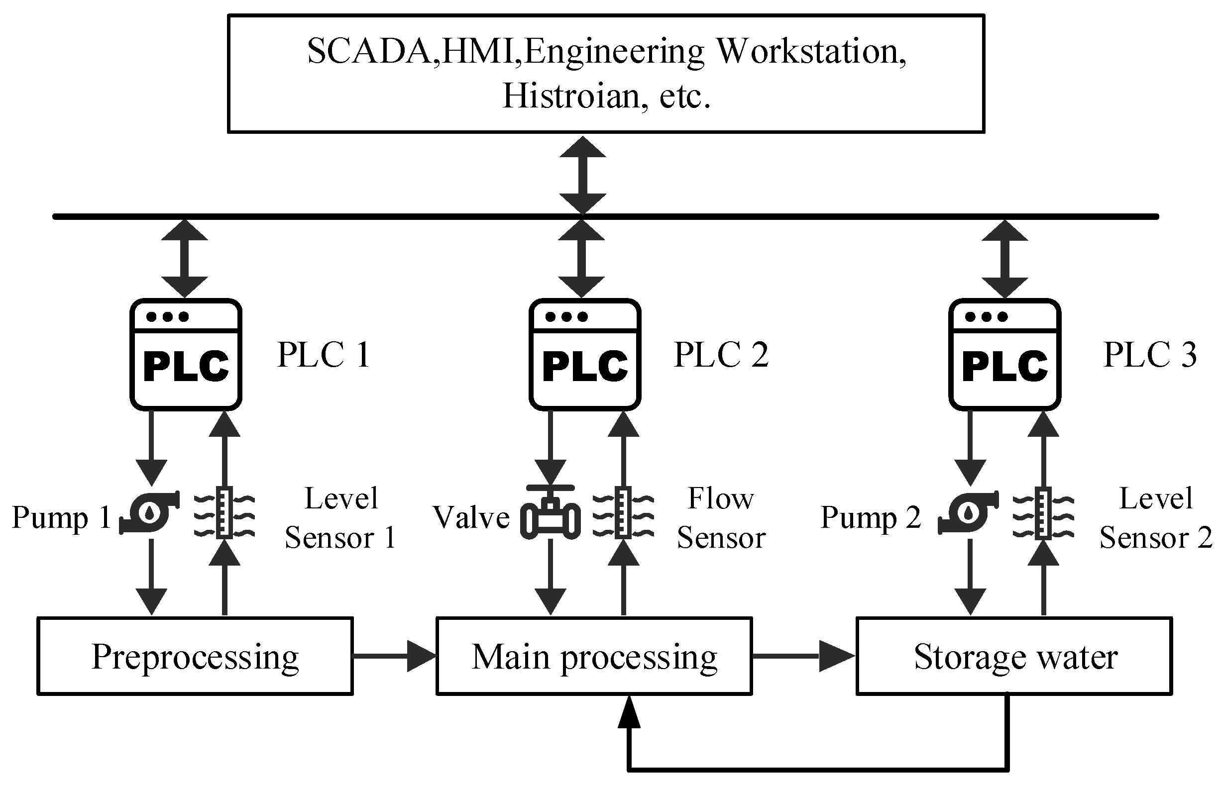
An illustrative example is provided later in Figure 1, where the storage tank’s water level remains stable, yet the upstream preprocessing pump continues operating despite no downstream demand. From a time-series perspective, the sensor values may seem normal, but this behavior violates expected inter-controller coordination logic—suggesting a potential fault or misconfiguration. Such anomalies cannot be effectively detected without explicitly modeling the dependencies among controllers and the physical process stages they govern.

The main contributions of this paper are as follows:

• We propose a novel framework, PCGAT, for anomaly detection in an ICS that explicitly models multi-level dependencies among physical processes, controllers, sensors, and actuators. The framework achieves superior performance on two public datasets.
• We introduce a structured multi-level graph that incorporates physical and control-layer information, allowing for a more accurate and interpretable representation of system dynamics.
• We conduct a case study demonstrating the interpretability of PCGAT, showing how attention weights reveal key behavioral patterns and decision rationales within the ICS.

2. Related Work

Anomaly detection methods for ICSs have significantly progressed in recent years. Research has mainly focused on methods based on deep learning and graph neural networks (GNNs). We discuss existing work from these two perspectives.

2.1. Anomaly Detection in ICS Based on Deep Learning

Deep learning methods have been widely applied in ICS anomaly detection due to their powerful feature extraction capabilities. For instance, the long short-term memory (LSTM) network-based method proposed by Kyle Hundman et al. [7] demonstrates strengths in handling time-series data; however, it suffers from issues related to long-term dependencies, and its efficiency declines significantly in training and inference when processing large datasets. The deep autoencoder-based method proposed by Bo Zong et al. [8] performed well on high-dimensional data. However, since its training relies on unsupervised learning, it is challenging to define clear boundaries between normal and abnormal samples, which leads to false positives or missed detections. Although the generative adversarial network (GAN) model of Dan Li et al. [9] can generate a variety of abnormal samples for detection, the training of GAN is usually unstable and may experience mode collapse, resulting in unsatisfactory anomaly detection results. The model based on a Transformer and dual temporal convolutional network (TCN) proposed by Lingrui Yu et al. [12] has significant advantages in capturing long-term dependencies. However, since the self-attention mechanism of the Transformer considers the global dependencies of all inputs, it may lead to insufficient modeling when processing large amounts of sensor data and ignore local correlations.

ICS anomaly detection methods based on deep learning have certain advantages in processing large-scale time series and high-dimensional data. Still, they often ignore the complex dependencies between sensors in industrial systems, lack sufficient interpretability, and struggle to meet the transparency requirements in industrial environments.

2.2. Anomaly Detection in ICS Based on Graph Neural Networks

GNNs can effectively model complex dependencies in ICSs and have gradually become a research hotspot in ICS anomaly detection. Although the complete graph structure proposed by Hang Zhao et al. [10] can ensure comprehensive connectivity between variables, constructing a complete graph in extensive systems results in substantial computational overhead. Ailin Deng et al.’s [11] graph construction method based on cosine similarity can learn potential relationships, but this method relies on the quality of sensor embedding. When the embedding is inaccurate or disturbed, the constructed graph structure may be incorrect, affecting the model’s anomaly detection ability. To improve the interpretability of the model, Chaofan Tang et al. [13] made improvements based on Ailin Deng et al. and added a gated recurrent network layer. Still, this method also increased the complexity of the model and required more computing resources during training. ICSs incorporate rich domain-specific prior knowledge. Weiqiang Wu et al. [14] introduced prior knowledge as graph regularization to learn a graph structure that conforms to the underlying physics and improves the interpretability of the model. However, such methods rely on accurate prior knowledge, but in actual industrial scenarios, prior information may be incomplete or noisy, resulting in limited model performance.

Overall, although the ICS anomaly detection method based on graph neural networks can better capture the dependencies between variables when facing large-scale complex systems, the efficiency and accuracy of the graph construction process and the graph structure are still urgent issues that need to be solved.

3. ICS and Problem Statement

This section introduces the industrial control system (ICS), discusses its multi-level dependencies, and presents the formal problem statement.

3.1. ICS

Figure 1 illustrates a simplified ICS architecture in a water treatment plant, where physical processes, controllers (PLCs), sensors, and actuators form a hierarchical dependency structure. The system consists of three stages—Preprocessing, Main Processing, and Water Storage—each governed by sensor–controller–actuator networks to ensure accurate and reliable operation.

The physical topology captures dependencies between adjacent processes, where actions in one stage directly influence the next. In parallel, the controller topology captures cross-stage communication, enabling coordinated control beyond local interactions.

For example, in the Preprocessing stage, Pump 1 draws water into the system, monitored by Level Sensor 1, which continuously transmits real-time data to PLC 1. Based on this input, PLC 1 adjusts the actuator of Pump 1 to maintain the target water level—forming a direct sensor–controller–actuator–process dependency loop.

In addition to local control, the system exhibits inter-process dependencies. Water from Preprocessing flows into Main Processing, meaning disruptions in one stage can propagate downstream. To manage such situations, the controller topology enables inter-stage coordination. For instance, if PLC 3 in the Water Storage stage detects a low water level, it can signal PLC 1 to increase Pump 1’s output, ensuring system-wide stability.

These sensor–controller–actuator–process relationships are summarized in

Table 1. Physical process and controller correspondence table.

Physical Process	Controller	Contain Sensors and Actuators
Preprocessing	PLC 1	Level Sensor 1, Pump 1
Main processing	PLC 2	Flow Sensor, Valve
Storage water	PLC 3	Level Sensor 2, Pump 2

. Based on this structured domain knowledge, we construct a graph-based model to effectively capture both local and global dependencies within the ICS.

3.2. Problem Statement

In an ICS, achieving production goals typically requires the coordinated operation of multiple sensors and actuators. Given the scarcity of anomalies in real-world production, this paper adopts an unsupervised method for ICS anomaly detection. Let $\mathrm{X}=[{\mathrm{x}}^{(1)},{\mathrm{x}}^{(2)},\dots ,{\mathrm{x}}^{(T_{\mathrm{train}})}]$ represent the normal training set, where $T_{\mathrm{train}}$ is the number of training samples. Each ${\mathrm{x}}^{(t)}={[x_1^{(t)},x_2^{(t)},\dots ,x_N^{(t)}]}^T$ denotes the values of all sensors and actuators at time t, where N is the number of sensors and actuators. The time-series data for the i-th sensor or actuator is represented by ${\mathrm{X}}_i=[x_i^{(1)},x_i^{(2)},\dots ,x_i^{(T_{\mathrm{train}})}]$. To enable unsupervised anomaly detection, we employ a prediction-based approach, where the goal is to forecast sensor values at the next timestamp based on historical data using a sliding window. The model takes historical data as input using a sliding window of size w, expressed as $S^{(t+1)}=[{\mathrm{x}}^{(t-w+1)},{\mathrm{x}}^{(t-w)},\dots ,{\mathrm{x}}^{(t)}]$. The model then outputs ${\widehat{\mathrm{x}}}^{(t+1)}\in {\mathbb{R}}^N$, representing the predicted sensor values at time $t+1$. The anomaly score at each timestamp is calculated by comparing the predicted value ${\widehat{\mathrm{x}}}^{(t+1)}$ with the observed value ${\mathrm{x}}^{(t+1)}$, thereby facilitating anomaly detection.

Beyond detecting anomalies, we analyze anomaly scores to pinpoint the specific sensors, actuators, or processes contributing to the issue. This offers engineers deeper insights into the root causes, facilitating fault diagnosis and system troubleshooting.

4. Methodology

4.1. Overall Framework

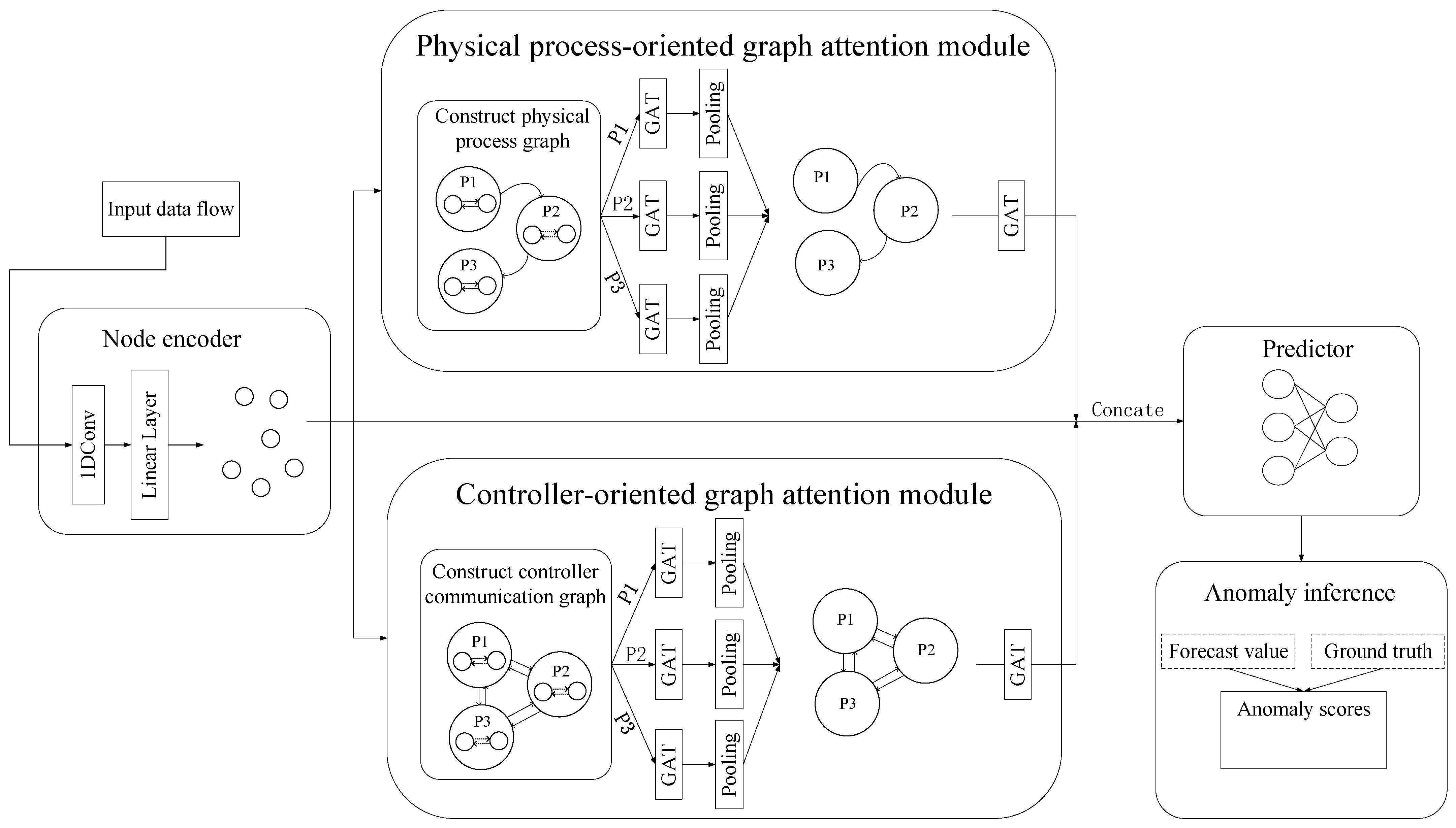
Figure 2 shows the proposed PCGAT architecture, which mainly includes the following parts: 1. Node encoder: used to learn and calculate the embedded representation of sensors and actuators. 2. Physical process-oriented graph attention network module: constructs a physical process graph based on the physical process information and extracts the spatial features of sensors and actuators through GAT. 3. Controller-oriented graph attention network module: constructs the controller communication graph based on the controller information and uses a GAT to capture the sensors and actuators information flow characteristics. 4. Predictor: obtains the representations of sensors and actuators through concatenation, and then predicts their values using a fully connected neural network. 5. Anomaly inference: calculates the anomaly score of sensors and actuators to perform anomaly judgment and location.

4.2. Graph Attention Network

The GAT aggregates features from neighboring nodes using learned attention coefficients. Given a graph $G=(V,E,X)$, where $V=\{v_1,v_2,\dots ,v_n\}$ is the set of nodes, $E=\{e_1,e_2,\dots ,e_m\}$ is the set of edges, and $X\in {\mathbb{R}}^{n\times k}$ is the node feature matrix, with n nodes and each node having a k-dimensional feature vector, the GAT adaptively assigns different attention weights to each neighbor.

The output feature of each node is calculated by the following formula:

$${\overline{x}}_i=\sigma (\sum _{j=1}^L{\alpha }_{ij}{x}_j)$$

(1)

where ${\overline{x}}_i$ represents the output feature of node i, and $\sigma$ represents the sigmoid activation function. ${\alpha }_{ij}$ represents the attention coefficient between nodes i and j, and node j is one of the neighboring nodes of node i. L is the number of neighboring nodes of node i.

The calculation method of attention coefficient ${\alpha }_{ij}$ is as follows:

$$e_{ij}=LeakyReLU({\omega }^{\top }·(x_i\oplus x_j)$$

(2)

$${\alpha }_{ij}={\displaystyle \frac{exp(e_{ij})}{{\displaystyle \sum _{l=1}^L}exp(e_{il})}}$$

(3)

where ⊕ means concatenating two node features, and $\omega \in {\mathbb{R}}^{2k}$ is a learnable weight vector. $LeakyReLU$ is a non-linear activation function. In this way, the GAT can adaptively adjust the feature aggregation process according to the importance of neighboring nodes to more effectively capture the complex relationship between nodes.

4.3. Node Encoder

The convolution operation has been shown to be effective for extracting local features within a sliding window [14]. In this approach, one-dimensional convolution is applied along the time dimension for each node’s input data within the sliding window. The resulting feature map is then vectorized and passed through a Linear layer to obtain the embedding vector for each node. This process can be formulated as follows for any node i:

$${\overline{x}}_i=Linear(Vec(Conv1D(x_i)))$$

(4)

where ${\overline{x}}_i$ represents the embedding vector of node i, with dimension $d_{emb}$, $Conv1D(·)$ represents the operation of one-dimensional convolution, $Vec(·)$ represents the operation of vectorization, and $Linear(·)$ represents the operation of linear mapping through the Linear layer.

4.4. Physical Process-Oriented Graph Attention Module

In an ICS, the relationships between sensors, actuators, and the physical processes they monitor are complex and hierarchical. While sensors and actuators provide localized measurements, the system’s overall behavior arises from both intra-process interactions among sensors and actuators, as well as inter-process dependencies across different stages. Capturing these multi-level dependencies is essential for effective anomaly detection. To address this, a multi-level graph structure is constructed to represent both local interactions within individual processes and global dependencies between processes, providing a comprehensive view of the entire system.

4.4.1. Construct Physical Process Graph

The initial sensor graph $G=(V,E)$ is defined with $V=\{v_1,v_2,\dots ,v_n\}$ representing the set of sensor nodes, where each node $v_i$ corresponds to the i-th sensor. To reflect the physical structure of the system, the node set V is divided into k subsets $\{V_1,V_2,\dots ,V_k\}$, where each subset $V_i$ contains the sensors associated with the i-th physical process.

Studies have shown strong correlations among sensors within the same physical process [15]. Therefore, each subset $V_i$ is used to construct a corresponding complete subgraph $G_i=(V_i,E_i)$, where every pair of sensor nodes within the same physical process is connected. This complete graph structure ensures that local interactions within each physical process are fully captured.

To model dependencies between different processes, a higher-level graph $H_1=(U_1,F_1)$ is constructed. Here, $U_1=\{G_1,G_2,\dots ,G_k\}$ represents the set of nodes, where each node corresponds to the embedded representation of a physical process subgraph. Edges in $F_1$ are established based on material or product flow paths in the industrial system, effectively capturing inter-process dependencies.

This multi-level graph structure integrates intra-process correlations and inter-process interactions, providing a comprehensive framework for modeling complex dependencies in an ICS and enhancing anomaly detection performance.

4.4.2. Multi-Level Physical Process Feature Extraction

After constructing the multi-level graph structure of the physical process, feature extraction is performed on graph structures at different levels. At the local level of the physical process, on each sensor subgraph $G_i$, a parallel GAT layer is applied. The GAT assigns weights to each node through an adaptive attention mechanism, focusing on aggregating information from essential neighboring nodes based on the correlation between their features. This operation captures the complex associations between sensors within the local scope of the physical process.

After feature extraction at the local level, the node features of each physical process subgraph $G_i$ are aggregated through mean pooling to generate an embedding vector representing the entire physical process. This operation effectively integrates the information between sensors within the physical process, resulting in a process-level feature representation. The embedding vector summarizes the relationships and information among sensors in the physical process.

At the global level, another layer of GAT operations is applied on the high-level physical process graph $H_1$. This GAT layer captures the global dependencies between different physical processes through an adaptive weighting mechanism. The embedding vector of each process serves as a node in the high-level graph. By leveraging the GAT, the model learns the interactions and dependencies between physical processes.

This multi-level feature extraction approach fully captures the complex dependencies among sensors and physical processes, enhancing the effectiveness of anomaly detection.

4.5. Controller-Oriented Graph Attention Module

In addition to physical processes, controllers in an ICS play a vital role in coordinating sensor operations and facilitating communication across the system. Each controller manages the internal flow of information from its associated sensors while also exchanging information with other controllers. Effectively capturing these interactions is crucial for maintaining system stability and ensuring reliable anomaly detection.

To model these dependencies, a multi-level graph structure is constructed to represent both intra-controller coordination and inter-controller communication. This structure provides a comprehensive view of local sensor relationships within each controller’s scope and the broader information flow across the entire system. By capturing these dependencies, the model effectively reflects the complex interactions required for robust anomaly detection.

4.5.1. Construction of the Controller Communication Graph

In an ICS, controllers interact through communication networks, forming dependencies that differ from those found in physical processes. To model these communication patterns, the node set V is divided into k subsets $\{V_1,V_2,\dots ,V_k\}$, where each subset $V_i$ contains sensors managed by the same controller.

For each subset $V_i$, a corresponding subgraph $G_i=(V_i,E_i)$ is constructed, where $E_i$ represents the communication links between sensors coordinated by the controller. As controllers are responsible for information flow and decision-making within their respective areas, each subgraph $G_i$ is modeled as a complete graph to capture the strong dependencies between sensors under the same controller’s management.

To capture system-wide coordination, a higher-level controller graph $H_2=(U_2,F_2)$ is constructed. Here, $U_2=\{G_1,G_2,\dots ,G_k\}$ represents the set of controller subgraphs, and $F_2$ denotes the edges representing communication links between controllers. These connections reflect the transmission of control signals and cooperative interactions required to maintain stable system operation.

4.5.2. Multi-Level Controller Feature Extraction

Feature extraction is conducted to capture both intra-controller coordination and inter-controller dependencies.

For each controller subgraph $G_i$, a GAT layer is applied to assign adaptive attention weights to sensor nodes. This mechanism emphasizes key interactions within the controller’s scope, allowing each sensor to incorporate relevant information from other sensors to improve local decision-making.

Next, the sensor features in each subgraph are aggregated using mean pooling, generating a condensed embedding vector that summarizes the controller’s overall behavior. To capture dependencies between controllers, a second GAT layer is applied to the controller graph $H_2$. Since this graph reflects system-wide communication patterns, the GAT operation allows the model to learn global coordination behaviors, further enhancing its ability to detect anomalies linked to signal transmission and collaborative control.

By jointly capturing local sensor coordination and global controller interactions, this multi-level feature extraction strategy effectively models complex dependencies within the ICS, improving the system’s ability to detect anomalies.

4.6. Predictor

To comprehensively represent each sensor’s features, we concatenate its initial embedding with the corresponding physical process and controller features. This approach ensures that each sensor’s representation encapsulates its intrinsic information and the broader local and global dependencies within the physical process and controller levels.

The concatenated features are then fed into a stacked, fully connected layer with an output dimension of N, representing the predicted values for N sensors at the next time step. This module leverages the integrated features to enhance prediction accuracy through a robust multi-level feature representation.

4.7. Training and Anomaly Detection Framework

During the training phase, the objective is to minimize the prediction error between the actual and predicted values. To quantify this error, the mean squared error is employed as the loss function:

$$L_{MSE}={\displaystyle \frac{1}{T_{train}-\omega }}\sum _{t=\omega +1}^{T_{train}}{∥{\widehat{s}}^t-s^t∥}_2^2$$

(5)

where ${\widehat{s}}^{(t)}$ denotes the predicted value at time t generated by the predictor, $s^{(t)}$ represents the ground truth value at time t, $\omega$ signifies the historical window size, and $T_{train}$ indicates the total length of the training time series.

For anomaly detection, discrepancies in the output layer’s predicted data are analyzed. Sensor anomalies typically manifest as significant deviations from normal behavioral patterns. This characteristic is exploited to compute an anomaly score for each sensor at time t using the following formulation:

$$Er{r}_i(t)=|s_i^{(t)}-{\widehat{s}}_i^{(t)}|$$

(6)

where $Er{r}_i(t)$ represents the absolute error of the ith sensor at time t. Due to varying sensitivities across different sensors and actuators, direct utilization of anomaly scores may obscure the anomalous behavior of certain sensors. To address this limitation, robust normalization is implemented on the error values of each sensor, thereby mitigating the influence of individual sensor variations:

$$a_i(t)={\displaystyle \frac{Er{r}_i(t)-{\tilde{\mu }}_i}{{\tilde{\sigma }}_i}}$$

(7)

where ${\tilde{\mu }}_i$ and ${\tilde{\sigma }}_i$ denote the median and quartile of the anomaly score $Er{r}_i(t)$ across the entire temporal domain, respectively.

To quantify the system’s overall state at time t, the maximum normalized anomaly score $A(t)$ across all sensors and actuators at that specific time point is utilized:

$$A(t)=\underset{i}{max}{a}_i(t).$$

(8)

Subsequently, by establishing a threshold $ϵ$, the system is classified as anomalous at time t when $A(t)>ϵ$. However, merely identifying a system anomaly is insufficient for implementing effective remediation measures. Therefore, the specific physical process is further localized through the sensor corresponding to the maximum anomaly score, enabling rapid identification of the anomaly source. For instance, if sensor 1 associated with process one exhibits the highest anomaly score, process one is determined to be malfunctioning and appropriate repair procedures are initiated. This approach eliminates the need for exhaustive investigations, thereby conserving valuable time and resources. Empirical evaluations demonstrate that this anomaly localization mechanism achieves substantial accuracy and efficiency in practical applications.

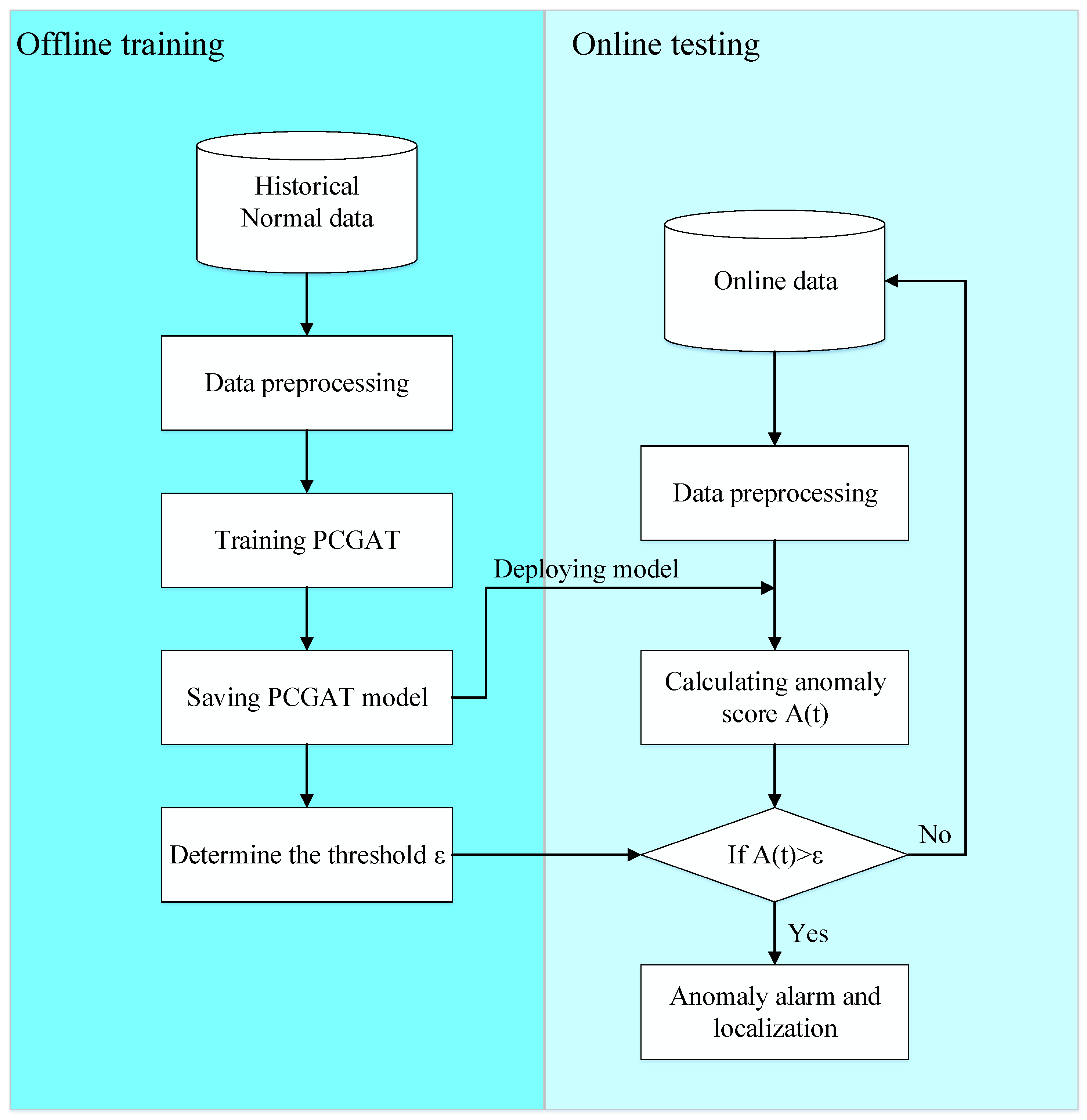
The overall workflow of the proposed PCGAT-based anomaly detection system is shown in Figure 3, which consists of offline training and online testing phases. During the offline phase, historical normal data are preprocessed and used to construct the physical process graph and controller communication graph. The PCGAT model is then trained to capture multi-level dependencies in the ICS, and an anomaly threshold $\epsilon$ is determined. In the online phase, real-time data are processed and fed into the trained PCGAT model to compute anomaly scores. If the score $A(t)$ exceeds $\epsilon$, an anomaly alarm is triggered and fault localization is performed.

This workflow supports practical deployment of PCGAT in ICS environments, such as water treatment systems, enabling accurate and interpretable anomaly detection.

5. Experiments

5.1. Dataset Description

We evaluated the performance of PCGAT using two real-world ICS datasets: Secure Water Treatment (SWaT) [16] and Water Distribution (WADI) [17] datasets, both provided by iTrust at the Singapore University of Technology and Design.

SWaT is a water treatment system with six interconnected processes: Water Supply, Chemical Dosing, Filtration, Dechlorination, Reverse Osmosis, and Storage. The dataset includes seven days of normal operations and four days of attack scenarios used for training and testing.

WADI is a scaled-down water distribution system with five main processes: Water Supply, Elevated Reservoir, Booster Station Consumer Tank, and Return Water. The WADI dataset contains 16 days of data, with the first 14 days under normal conditions and the final 2 days containing attack scenarios.

To streamline training, we downsampled both datasets to one data point per 10 s by averaging the original readings, while the labels represent the most frequent label during the 10 s window. Max–min normalization was applied for preprocessing, and the training data were split into a training set (90%) and a validation set (10%).

Table 2. Dataset information.

Dataset	Number of Sensors	Number of Processes	Number of Controllers	Number of Anomalies	Number of Training Samples
SWaT	51	6	6	36	496,800
WADI	123	5	5	24	1,187,950

summarizes key dataset statistics.

5.2. Experimental Settings

5.2.1. Baselines and Evaluation Metrics

To verify the proposed method’s effectiveness, we compared it with several representative anomaly detection methods, including LSTM-NDT [7], DAGMM [8], MAD-GAN [9], GDN [11], DTAAD [12], and GRN [13].

The performance of all methods was assessed using four standard anomaly detection metrics: precision (Prec), recall (Rec), F1 score (F1), and the area under the ROC curve (AUC). Precision measures how many detected anomalies are correct, while recall evaluates the model’s ability to identify all actual anomalies. The F1 score combines precision and recall into a single value, reflecting overall detection performance. AUC provides a broader evaluation by measuring the model’s ability to distinguish between normal and abnormal instances across various thresholds. Given the imbalanced nature of the datasets, with relatively fewer anomalies, we prioritized the F1 score and AUC for a more comprehensive assessment of detection effectiveness.

5.2.2. Experimental Environment and Parameter Settings

All experiments were conducted on a machine equipped with an Intel (R) Xeon (R) Gold 5318Y CPU @ 2.10 GHz (Intel Corporation, Santa Clara, CA, USA) and an NVIDIA A800 GPU (NVIDIA Corporation, Santa Clara, CA, USA). The implementation was based on PyTorch 1.10.0 with CUDA version 11.3.1. The models were trained using the Adam optimizer with a learning rate of 0.005 and $({\beta }_1,{\beta }_2)=(0.9,0.99)$. An early stopping strategy was adopted, with a maximum of 50 training epochs and a patience of 10.

For the SWaT dataset, time-series data were processed using a sliding window with a window size of 5 and a step size of 1. Feature embeddings were generated by a one-dimensional convolution layer with a kernel size of 5, and the embedding dimension was set to 32. The output layer of the model contained 128 neurons.

For the WADI dataset, to improve training efficiency, the sliding window size was increased to 10 and the step size to 3. The kernel size of the convolution layer was set to 9, and the embedding dimension remained 32. The output layer consisted of 64 neurons.

5.3. Overall Performance

Table 3. Anomaly detection results on SWaT and WADI datasets.

Model	SWaT				WADI
	Prec	Rec	F1	AUC	Prec	Rec	F1	AUC
LSTM-NDT	0.9999	0.0109	0.0215	0.5054	0.4073	0.3910	0.3990	0.6887
DAGMM	0.9955	0.6879	0.8136	0.8437	0.2747	0.8296	0.4127	0.8889
MAD-GAN	0.9977	0.6879	0.8143	0.8439	0.4906	0.3910	0.4351	0.6907
GDN	0.9958	0.6523	0.7884	0.8738	0.4832	0.4145	0.4460	0.8032
DTAAD	0.9977	0.6879	0.8143	0.8439	0.6047	0.3910	0.4749	0.6925
GRN	0.9956	0.6521	0.7881	0.8751	0.9362	0.3211	0.4778	0.8090
PCGAT	0.9808	0.7550	0.8533	0.9129	0.7162	0.3688	0.4866	0.8753

presents the anomaly detection results of each model on the SWaT and WADI datasets.

On the SWaT dataset, PCGAT achieved the highest F1 score of 0.8533 and AUC of 0.9129, significantly outperforming existing state-of-the-art methods. Compared to MAD-GAN and DTAAD (both achieving an F1 score of 0.8143), PCGAT improved the F1 score by 0.039 (4.8%), indicating its superior ability to balance precision and recall. In terms of AUC, PCGAT surpassed GRN (0.8751) by 0.0378 (4.3%), reflecting better overall discrimination between normal and anomalous states.

Notably, although LSTM-NDT achieved the highest precision (0.9999) on SWaT, its extremely low recall (0.0109) led to a poor F1 score (0.0215), underscoring the importance of balanced evaluation metrics in practical scenarios. In contrast, PCGAT maintained a high precision (0.9808) while achieving the highest recall (0.7550), demonstrating its effectiveness in detecting a larger proportion of anomalies without significantly increasing false positives.

The WADI dataset presents a more challenging scenario due to its higher dimensionality and more pronounced class imbalance. Despite these challenges, PCGAT maintained robust performance, achieving the highest F1 score (0.4866) among all methods, slightly outperforming GRN (0.4778) by 0.0088 (1.8%). While DAGMM achieved the highest AUC (0.8889), surpassing PCGAT (0.8753) by 0.0136 (1.5%), this minor advantage was offset by DAGMM’s substantially lower F1 score (0.4127).

PCGAT also achieved the highest precision (0.7162) on the WADI dataset, with the exception of GRN (0.9362), which obtained higher precision at the cost of significantly lower recall. This high precision is particularly valuable in industrial control systems, where false alarms can cause unnecessary operational disruptions and maintenance costs.

Overall, PCGAT demonstrated consistent performance across both datasets, highlighting its robustness and generalizability in diverse ICS environments. These results provide strong empirical evidence that incorporating domain knowledge of physical processes and control mechanisms into a graph attention architecture enables more accurate modeling of system behavior and improves anomaly detection capabilities.

5.4. Ablation Experiments

This section conducts ablation experiments on the SWaT and WADI datasets to verify the effectiveness of each component of PCGAT, including the physical process-oriented graph attention module, the controller-oriented graph attention module, and the one-dimensional convolution layer. The experimental settings of this experiment are consistent with the previous experiments. As shown in

Table 4. Ablation results on SWaT and WADI datasets.

Model	SWaT				WADI
	Prec	Rec	F1	AUC	Prec	Rec	F1	AUC
PCGAT	0.9808	0.7550	0.8533	0.9129	0.7162	0.3688	0.4866	0.8753
w/o Physical process-oriented graph attention module	0.9889	0.6153	0.7585	0.8540	0.2819	0.3290	0.3035	0.7496
w/o Controller-oriented graph attention module	0.8312	0.7351	0.7803	0.8841	0.1178	0.3439	0.1755	0.6483
w/o one-dimensional convolution	0.2005	0.8112	0.3216	0.6282	0.8454	0.1740	0.2883	0.7493

, each component significantly contributes to the overall model performance.

First, removing the physical process-oriented graph attention module results in lower F1 scores and AUC values on both the SWaT and WADI datasets. This demonstrates that modeling dependencies among physical processes are critical for accurately capturing abnormal patterns. Second, when the controller-oriented graph attention module is removed, all performance metrics decline, indicating that inter-controller communication is also essential for effective anomaly detection. Finally, removing the one-dimensional convolution layer, which captures local temporal dependencies, leads to a significant drop in detection performance. This highlights the importance of temporal features in industrial systems, where 1D convolution effectively extracts local sensor-level patterns.

5.5. Effects of Training Set Size

To assess how the amount of training data influences model performance, we trained PCGAT using 20%, 40%, 60%, 80%, and 100% of the training set, while keeping the test set fixed across all experiments. This analysis provides insight into the data efficiency of our method and helps determine the minimum training data required for satisfactory detection accuracy. The results are summarized in

Table 5. Effect of training set size on model performance across different datasets.

Dataset	Metric	Training Set Size
		20%	40%	60%	80%	100%
SWaT	Prec	0.9385	0.9707	0.4020	0.9694	0.9808
	Rec	0.7223	0.6040	0.7176	0.6827	0.7550
	F1	0.8165	0.7448	0.5153	0.8011	0.8533
	AUC	0.8675	0.8433	0.8246	0.8742	0.9129
WADI	Prec	0.7440	0.7038	0.5196	0.8023	0.7162
	Rec	0.1531	0.3141	0.3032	0.1372	0.3688
	F1	0.2537	0.4354	0.3827	0.2341	0.4866
	AUC	0.5558	0.8116	0.6740	0.5566	0.8753

.

For the SWaT dataset, performance does not increase monotonically with more training data. While the best results are achieved with the full training set (F1 score of 0.8533 and AUC of 0.9129), the model still performs well with only 20% of the data (F1 score of 0.8165). Notably, a significant drop in precision is observed at 60% (0.4020), which negatively affects the F1 score. This non-linear trend suggests that the representativeness of the training data may be more important than sheer quantity for this dataset.

In contrast, the WADI dataset shows a stronger dependence on the amount of training data. The best performance is obtained using the full training set (F1 score of 0.4866 and AUC of 0.8753), reflecting the need for more data in this more complex system. However, the performance trend remains non-linear, with 40% training data yielding the second-best results (F1 score of 0.4354 and AUC of 0.8116). The overall lower performance on WADI compared to SWaT highlights the increased difficulty of anomaly detection in more intricate water distribution systems.

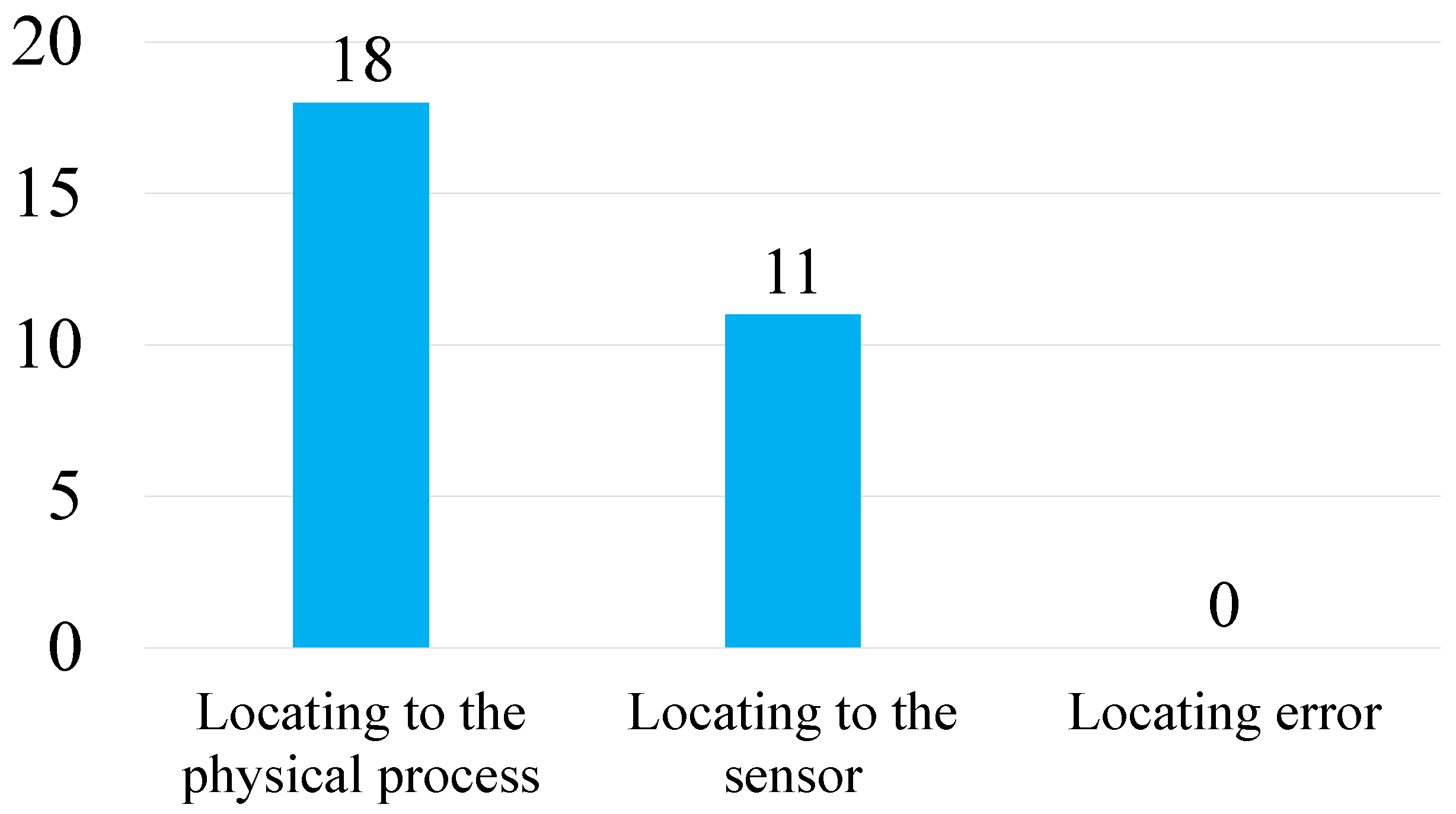
5.6. Anomaly Localization Capability

In this section, we evaluate the anomaly localization capability of the proposed method on the SWaT dataset, which contains 36 known anomaly events. Among these, our model successfully detected 18 events. As shown in Figure 4, PCGAT not only identified the anomalies but also accurately located the corresponding physical processes for the 18 successfully detected events.

Further analysis reveals that, for 11 of these cases, the model could precisely identify the specific sensor where the anomaly occurred—the sensor with the highest anomaly score matched the ground-truth anomalous sensor. This capability is particularly valuable in complex ICS environments, as it enables rapid problem localization and targeted response measures, thereby reducing troubleshooting time and enhancing the safety and stability of system operations.

5.7. Graph Attention-Based Anomaly Detection Explanation

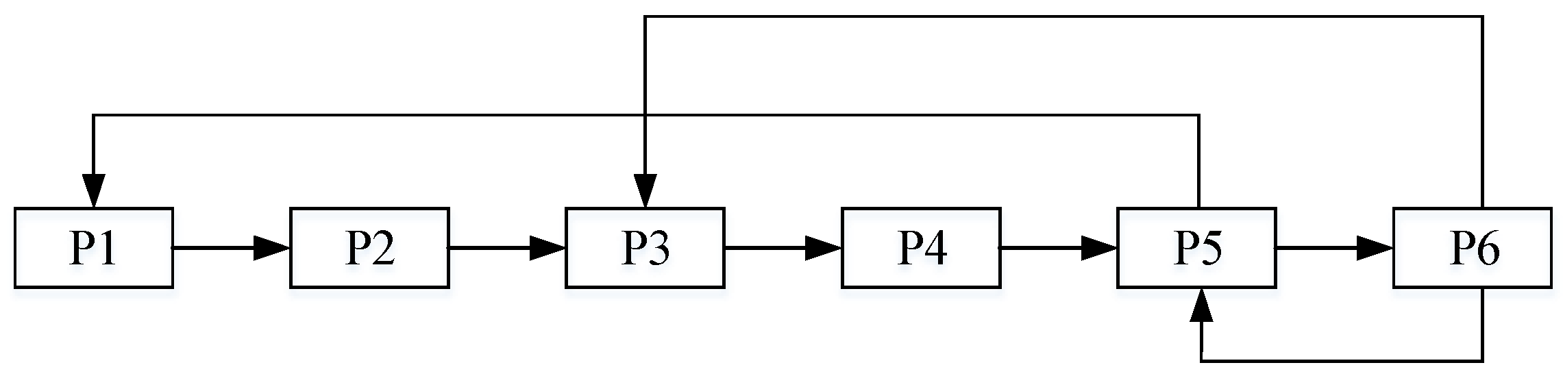
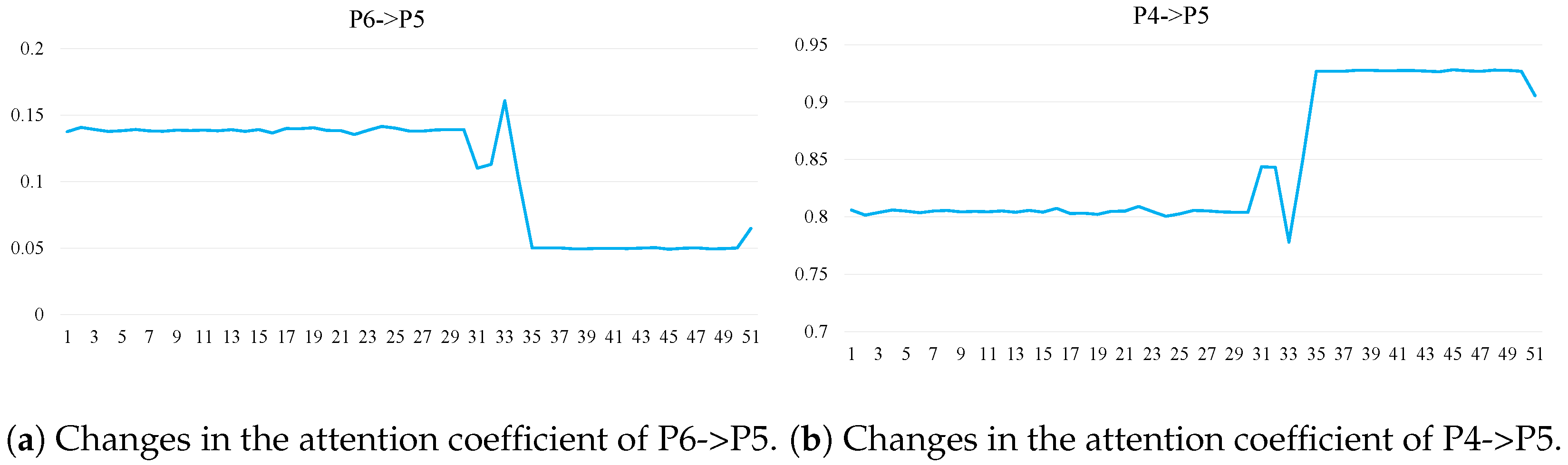
To further illustrate how the GAT layer on the physical process graph enhances anomaly detection, we analyze a representative anomaly case from the SWaT dataset. The SWaT physical process graph is shown in Figure 5 [18]. We visualize the parts of the graph where attention coefficients change significantly in Figure 6. The first 30 timestamps represent normal conditions (sensor AIT-202 readings > 7.05), after which an anomaly is introduced by setting AIT-202 to a fixed value of 6.

The results show that the attention coefficients between Dechlorination (P4) and Reverse Osmosis (P5), as well as those between P6 and P5, remain stable during the normal period. However, once the anomaly occurs, these attention coefficients fluctuate significantly. The anomaly is caused by a tampering attack on sensor AIT-202, which measures pH values. The original reading above 7.05 is artificially reduced to 6, indicating increased water acidity.

This change in water quality directly affects the performance of Dechlorination (P4), resulting in abnormal output water, which then enters the RO system (P5). As the RO system is sensitive to water quality, the GAT increases the attention from P4 to P5 to reflect the increased influence. Simultaneously, due to the water quality issue, the flow from P5 to P6 decreases, leading to reduced backflow from P6 to P5. Accordingly, the GAT dynamically lowers the attention on the P6-to-P5 path.

This analysis demonstrates that the GAT layer can adaptively adjust attention weights between different physical processes in response to anomalies, thereby enhancing both the detection accuracy and interpretability of the model.

6. Conclusions

This paper proposes a novel method, PCGAT, for anomaly detection in an ICS. By integrating the graph structural information of physical processes with controller communications, PCGAT effectively captures multi-level dependencies in complex systems. Experimental results demonstrate that PCGAT significantly improves anomaly detection performance on the SWaT and WADI datasets, particularly in anomaly localization, where it can accurately identify the affected physical processes. Ablation studies further confirm the effectiveness of each component of the model. Specifically, the graph attention layers for physical processes and controllers, as well as the use of one-dimensional convolution to extract local temporal dependencies, contribute substantially to the overall performance.

Given that industrial systems operate under diverse conditions that may vary over time and across environments, future work will explore the deployment of PCGAT in real-time settings. In particular, we aim to investigate how to incorporate online learning capabilities into the model, enabling it to dynamically adjust to system changes and enhance real-time anomaly detection and localization.