Finite-Time Control for Maneuvering Aircraft with Input Constraints and Disturbances

Abstract

In this paper, a finite-time control method integrating a high-order disturbance observer (HODO) and a finite-time auxiliary system (FTAS) is proposed for maneuvering aircraft under disturbances and input constraints. To attenuate the adverse effects of disturbances, the HODOs were designed to obtain their estimations, which were then incorporated into the control channel as feedforward compensation. To solve the issue of input constraints, a novel FTAS was developed to ensure effective control performance. To achieve rapid attitude tracking for maneuvering aircraft and address the issue of singularity caused by the virtual control derivative, finite-time control with a piecewise function technique was employed. Furthermore, the stability analysis of the closed-loop system was conducted through Lyapunov stability theory. Finally, the efficacy of the proposed control method was demonstrated by simulation results.

1. Introduction

In recent years, with the implementation of thrust vector engines [1,2] and advances in aerodynamic characteristic theories [3,4], the flight envelopes of aircraft have gradually expanded to include low-speed and high-angle-of-attack (HAOA) regions. Based on the substantial expansion of the flight envelope and advancements in flight maneuver control technologies, aircraft can now rapidly change their attitude over a wide range. These advancements have significantly increased flexibility in enhancing aircraft maneuverability, further enabling agile evasion and the attainment of advantageous positions. Owing to these benefits, aircraft maneuvering control has become a prominent research focus [5,6,7,8]. Nevertheless, several issues persist, including disturbances, control input constraints, and the need for rapid attitude angle tracking, all of which continue to make maneuvering flights a challenging task. Thus, further investigation into aircraft maneuvering control is imperative.

During the flight maneuver, the aircraft is highly sensitive to changes in attitude. Even slight variations in attitude can potentially induce abrupt changes in aerodynamic characteristics, leading to the deterioration of in-flight performance. Moreover, due to the intrinsic characteristics and the complex external environment during the maneuver, the aircraft is inevitably subject to various disturbances that drive the attitude of the aircraft in unpredictable evolutions, thereby posing risks to flight safety. To deal with the challenge of disturbances, several robust control methods, such as the sliding mode control [9,10], the $H_{\infty }$ [11,12], and the disturbance observer method [13,14], have been developed. Distinct from sliding mode control and $H_{\infty }$ methods, which are generated based on the passive anti-disturbance idea, the disturbance observer is an active anti-disturbance method. By actively estimating disturbances and feeding forward the estimates into the control channel, the detrimental influence of the disturbances on the controlled system can be suppressed. This capability makes disturbance observers highly versatile and easily integrable with various control methods. For instance, [15] applied a disturbance observer in the backstepping method, together with a radial basis neural network, for position control of the reconfigurable variable stiffness actuator in environments characterized by disturbances and system uncertainty. In [16], the disturbance observer was used in the model predictive control for the speed consistency of multi-linear motor traction systems. In addition, the disturbance observer has also been used in control systems for maneuvering flights. In [17], the disturbance observer was designed to realize the robust post-stall pitching maneuver for the aircraft against unsteady aerodynamic disturbances. In [18], a switched prescribed performance method was developed, utilizing a disturbance observer to achieve HAOA maneuverability for aircraft facing external disturbances. Furthermore, based on the disturbance observer technique, the high-order disturbance observer (HODO) has been proposed for more general systems with disturbances [19,20]. However, the application of HODO in the control of maneuvering aircraft remains relatively unexplored, motivating the research presented in this paper.

It is worth emphasizing that the key aspect of maneuvering aircraft is the rapid tracking of attitude angles. Finite-time control, known for its ability to drive the system states to converge within a finite time, aligns well with the requirement for rapid tracking. Specifically, under finite-time control, the dynamics with the finite-time convergence property can be flexibly constructed by incorporating an appropriate fractional order into the control law, making finite-time control a widely adopted approach in various applications. For example, in [21], a finite-time formation-containment control was developed for ground–air coordination. In [22], a robust finite-time composite learning control method was proposed with the parameter adaptive technique for master–slave network nonlinear telerobotics systems. Moreover, in view of the fact that the dynamics for maneuvering aircraft can be in the affine nonlinear form, it is convenient to integrate finite-time control into the backstepping control scheme. In [23], finite-time control and the adaptive backstepping method were investigated together with the barrier Lyapunov function for strict-feed systems with state constraints. In [24], the backstepping-based finite-time control method was used for trajectory tracking for the surface vessel. By embedding finite-time control into the cascade structure of the backstepping design, step by step, backstepping-based finite-time control can be easily obtained. Nevertheless, the derivative operation of the virtual control law with the order from 0 to 1 was carried out, resulting in the challenging singularity problem. Thus, further advancements are needed to improve backstepping-based finite-time control.

Another critical issue for maneuvering aircraft that warrants attention is the input constraints. In practical engineering applications, the physical structure of the actuator mechanism imposes limitations on the deflection capabilities of the thrust vectoring engine and control surfaces, restricting the operational range for these actuators. At the same time, the rapid and wide-ranging attitude adjustments characteristic of maneuvering aircraft further exacerbate the issue of input constraints. To solve this issue, the auxiliary system was developed [25,26,27,28]. By accounting for the differences between constrained and unconstrained inputs in the system states and designing a controller accordingly, the negative impacts of input constraints can be effectively mitigated. In [29], considering elevator deflection saturation, an auxiliary system was employed in the trajectory tracking controller for the boost-glide vehicle. In [30], considering the constrained forces and moments, an auxiliary system was introduced to lessen the tracking error’s dependence on the input amplitude for quadrotor unmanned aerial vehicles. Furthermore, the auxiliary system has been incorporated into finite-time control [31,32,33,34]. Inspired by the works mentioned above, it seems promising to employ the auxiliary system in finite-time control for aircraft maneuverability.

The objective of this paper is to enable HAOA aircraft maneuverability control subject to disturbances and input constraints so that the flight speed can be decreased to realize evasion ability and attack situations. To achieve this motivation, a finite-time control method combined with HODO and a finite-time auxiliary system (FTAS) was developed within the backstepping control scheme. The HODO was designed to mitigate the negative influences of disturbances and reduce dependence on the control parameters within the control matrix. The FTAS was developed to counteract the detrimental effects caused by input constraints. The primary contributions of this paper are outlined as follows:

• A finite-time control law using a piecewise function technique was designed for controlling aircraft during flight maneuvers. In this way, the singularity issue of the backstepping-based finite-time control can be addressed.
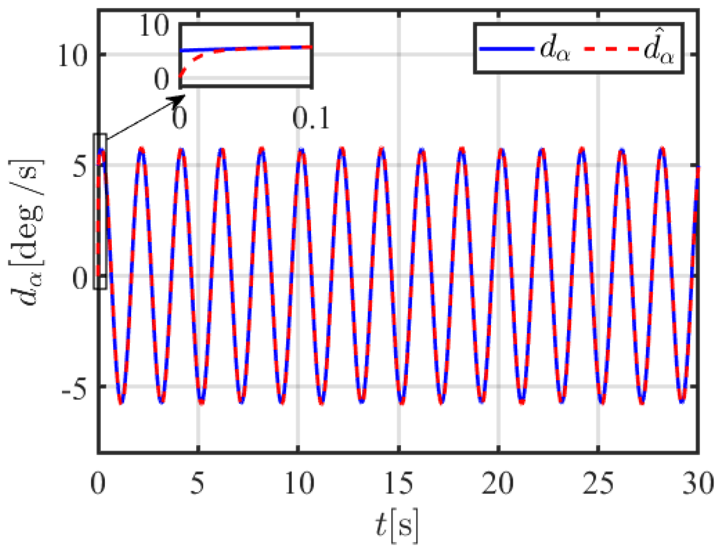
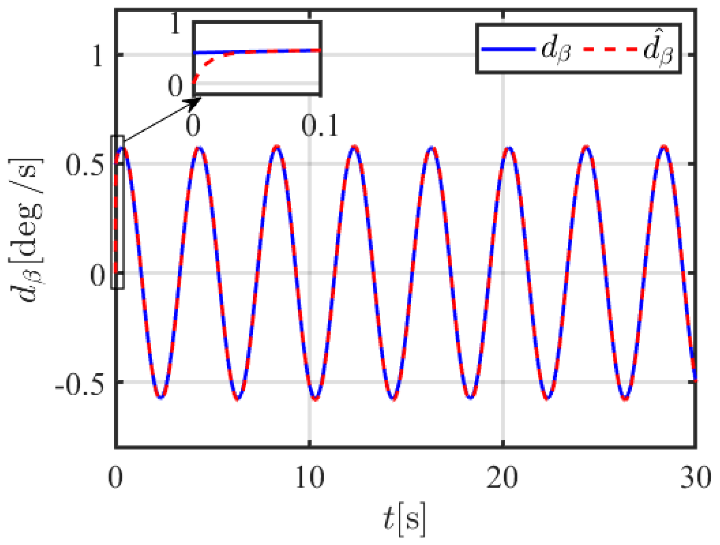
• A HODO was designed to estimate disturbances during the maneuvering of aircraft. With this technique, the disturbance estimates can be fed forward into the control channel to effectively mitigate their adverse impacts.
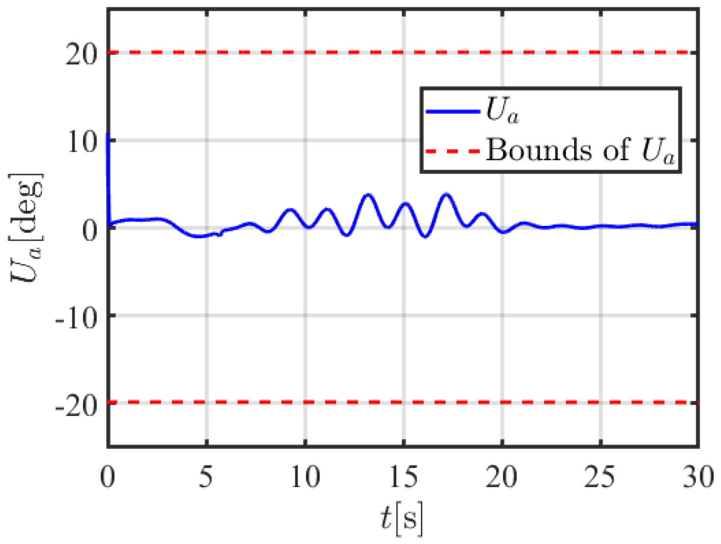
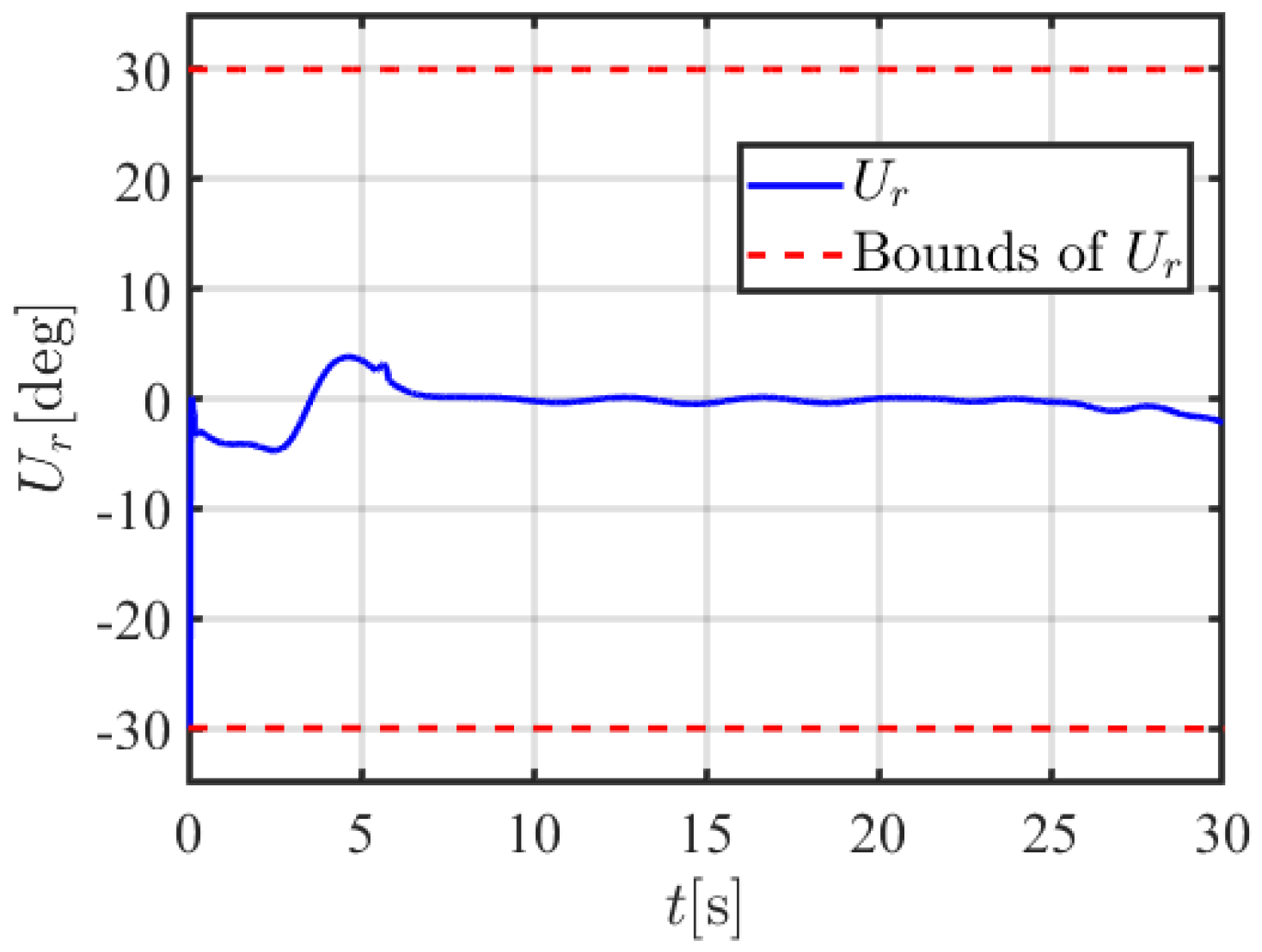
• A novel FTAS was developed by introducing the control matrix into the design. By this means, this approach suppresses the adverse effects of input constraints on system performance and reduces the dependency on control parameters on the control matrix.

This paper is constructed as follows. Section 2 formally introduces the problem formulation. Section 3 presents the comprehensive design for the HODO-based finite-time control, which is verified by the simulation results in Section 4. Finally, this paper is concluded in Section 5.

Notation 1. 

Let $\mathbb{R}$ denote the real number set, $\mathbf{I}$ denote the identity matrix, and 0 denote the zero matrix. For a scalar $a\in \mathbb{R}$, $\mathrm{sign}\left(a\right)=1$ if $a>0$, $\mathrm{sign}\left(a\right)=0$ if $a=0$, and $\mathrm{sign}\left(a\right)=-1$ if $a<0$. For a scalar $b\in \mathbb{R}$, ${⌈a⌋}^b=\mathrm{sign}\left(a\right){\left|a\right|}^b$. $0^{+}$ denotes the infinitesimal positive number. Let ${\mathbb{R}}^n$ denote the n-dimensional real vector set. For a vector $\mathit{A}={\left[a_1,a_2,\cdots ,a_n\right]}^{\top }\in {\mathbb{R}}^n$, ${⌈\mathit{A}⌋}^b={\left[{⌈a_1⌋}^b,{⌈a_2⌋}^b,\cdots ,{⌈a_n⌋}^b\right]}^{\top }$. For a matrix $\mathit{B}$, ${\mathit{B}}^{m\times n}$ denotes the matrix with m rows and n columns, ${\mathit{B}}^{\top }$ denotes the transpose of $\mathit{B}$, ${\parallel \mathit{B}\parallel }_F$ denotes the Frobenius norm of $\mathit{B}$, $\mathbf{diag}\{•\}$ denotes the diagonal matrix, and ${\lambda }_{min}\{•\}$ denotes the minimum eigenvalue.

2. Problem Formulation

The attitude dynamics equations for maneuvering aircraft, which can be written in affine nonlinear form, are given as follows [17]:

$$\left\{\begin{array}{c}{\dot{\mathit{x}}}_1={\mathit{F}}_1\left({\mathit{x}}_1\right)+{\mathit{G}}_1\left({\mathit{x}}_1\right){\mathit{x}}_2+{\mathit{d}}_1\left(t\right)\hfill \\ {\dot{\mathit{x}}}_2={\mathit{F}}_2\left({\mathit{x}}_1,{\mathit{x}}_2\right)+{\mathit{G}}_2\left({\mathit{x}}_1,{\mathit{x}}_2\right)\mathit{U}\left(\mathit{u}\right)+{\mathit{d}}_2\left(t\right)\hfill \end{array}\right.$$

(1)

where ${\mathit{x}}_1={\left[\alpha ,\beta ,\mu \right]}^{\top }$ denotes the attitude angle vector with $\alpha$, $\beta$, and $\mu$ denoting the angle of attack, the sliding angle, and the flight-path roll angle, respectively, ${\mathit{x}}_2={\left[p,q,r\right]}^{\top }$ denotes the attitude angular rates vector with p, q, and r denoting the roll, pitch, and yaw angular rates, respectively, ${\mathit{F}}_1={[F_{\alpha },F_{\beta },F_{\mu }]}^{\top }$ and ${\mathit{F}}_2={[F_p,F_q,F_r]}^{\top }$ denote the dynamic function vectors, ${\mathit{G}}_1$ and ${\mathit{G}}_2$ denote the control matrices, ${\mathit{d}}_1={[d_{\alpha },d_{\beta },d_{\mu }]}^{\top }$ and ${\mathit{d}}_2={[d_p,d_q,d_r]}^{\top }$ denote the disturbances vectors, $\mathit{U}\left(\mathit{u}\right)={\left[U_a\left(u_a\right),U_r\left(u_r\right),U_y\left(u_y\right),U_z\left(u_z\right)\right]}^{\top }$ denotes the constrained control input vector, $U_a$ and $U_r$ denote the aileron and rudder deflection angles, respectively, $U_y$ and $U_z$ denote the thrust vectoring lateral and normal deflection angles, respectively, and $\mathit{u}={\left[u_a,u_r,u_y,u_z\right]}^{\top }$ denotes the corresponding unconstrained control input vector to be designed. ${\mathit{G}}_1$ and ${\mathit{G}}_2$ are detailed as follows [17]:

$${\mathit{G}}_1=\left[\begin{array}{ccc}-tan\beta cos\alpha & 1& -tan\beta sin\alpha \\ sin\alpha & 0& -cos\alpha \\ sec\beta cos\alpha & 0& sec\beta sin\alpha \end{array}\right],{\mathit{G}}_2=\left[\begin{array}{cccc}{g}_{p,U_a}& g_{p,U_r}& g_{p,U_y}& 0\\ 0& 0& 0& g_{q,U_z}\\ g_{r,U_a}& g_{r,U_r}& g_{r,U_y}& 0\end{array}\right]$$

(2)

where $g_{p,U_a}={\displaystyle \frac{I_{zz}{\overline{q}}_f{S}_f{b}_f{C}_{l,U_a}\left({\alpha }_u\right)}{I_{xx}{I}_{zz}-{\left(I_{xz}\right)}^2}}+{\displaystyle \frac{I_{xz}{\overline{q}}_f{S}_f{b}_f{C}_{n,U_a}\left({\alpha }_u\right)}{I_{xx}{I}_{zz}-{\left(I_{xz}\right)}^2}}$, $g_{p,U_r}={\displaystyle \frac{I_{zz}{\overline{q}}_f{S}_f{b}_f{C}_{l,U_r}\left({\alpha }_u\right)}{I_{xx}{I}_{zz}-{\left(I_{xz}\right)}^2}}+{\displaystyle \frac{I_{xz}{\overline{q}}_f{S}_f{b}_f{C}_{n,U_r}\left({\alpha }_u\right)}{I_{xx}{I}_{zz}-{\left(I_{xz}\right)}^2}}$, $g_{p,U_y}=-{\displaystyle \frac{\pi I_{xz}{\overline{x}}_f{T}_f}{180\left(I_{xx}{I}_{zz}-{\left(I_{xz}\right)}^2\right)}}$, $g_{q,U_z}={\displaystyle \frac{\pi {\overline{x}}_f{T}_f}{180I_{yy}}}$, $g_{r,U_a}={\displaystyle \frac{I_{xz}{\overline{q}}_f{S}_f{b}_f{C}_{l,U_a}\left({\alpha }_u\right)}{I_{xx}{I}_{zz}-{\left(I_{xz}\right)}^2}}+{\displaystyle \frac{I_{xx}{\overline{q}}_f{S}_f{b}_f{C}_{n,U_a}\left({\alpha }_u\right)}{I_{xx}{I}_{zz}-{\left(I_{xz}\right)}^2}}$, $g_{r,U_r}={\displaystyle \frac{I_{xz}{\overline{q}}_f{S}_f{b}_f{C}_{l,U_r}\left({\alpha }_u\right)}{I_{xx}{I}_{zz}-{\left(I_{xz}\right)}^2}}+{\displaystyle \frac{I_{xx}{\overline{q}}_f{S}_f{b}_f{C}_{n,U_r}\left({\alpha }_u\right)}{I_{xx}{I}_{zz}-{\left(I_{xz}\right)}^2}}$, $g_{r,U_y}=-{\displaystyle \frac{\pi I_{xx}{\overline{x}}_f{T}_f}{180\left(I_{xx}{I}_{zz}-{\left(I_{xz}\right)}^2\right)}}$, $I_{xx}$, $I_{yy}$, and $I_{zz}$ denote the moments of inertia around the x-axis, y-axis, and z-axis, respectively, $I_{xz}$ denotes the product of inertia with respect to the $x–z$ plane, ${\overline{q}}_f={\displaystyle \frac{1}{2}}{\rho }_f{\displaystyle V_f^2}$ denotes the dynamic pressure, ${\rho }_f$ denotes the air density, $V_f$ denotes the aircraft flight speed, $S_f$ denotes the reference surface area of the wing, $b_f$ denotes the wingspan, ${\overline{x}}_f$ denotes the distance between the center of mass and the engine nozzle, $T_f$ denotes the thrust $C_{l,U_a}$, $C_{n,U_a}$, $C_{l,U_r}$, and $C_{n,U_r}$ denote the aerodynamic coefficients.

The dynamics of the flight speed is given as follows [17]:

$${\dot{V}}_f={\displaystyle \frac{T_{f}cos\alpha }{M_f}}+{\displaystyle \frac{\pi T_f{U}_{z}sin\alpha }{180M_f}}-{\displaystyle \frac{{\rho }_f{\displaystyle V_f^2}{S}_f{C}_D}{2M_f}}-gsin{\gamma }_f$$

(3)

where $M_f$ denotes the mass of the aircraft, $C_D$ denotes the drag force aerodynamic coefficient, g denotes the acceleration of gravity, and ${\gamma }_f$ denotes the flight tilt angle of the aircraft.

The constrained control inputs are detailed as follows [18]:

$$U_i\left(u_i\right)=\left\{\begin{array}{cc}{B}_i\mathrm{sign}\left(u_i\right),\hfill & \hfill \mathrm{if}\left|u_i\right|>B_i\\ u_i,\hfill & \hfill \mathrm{if}\left|u_i\right|\le B_i\end{array}\right.$$

(4)

where $\forall i\in \{a,r,y,z\}$, and $B_i$ denotes the constrained bound of $u_i$.

Remark 1. 

In a traditional flight, maneuvering is difficult to control using the aileron and rudder deflection angles $U_a$ and $U_r$, as well as the thrust $T_f$. In this paper, to achieve HAOA maneuverability, thrust vectoring is applied to the aircraft through the lateral and normal deflection angles $U_y$ and $U_z$. Nevertheless, the deflection angles $U_a$, $U_r$, $U_y$, and $U_z$ are limited, which has motivated the research presented in this paper.

To proceed further, the lemmas and assumptions are required as follows:

Lemma 1 

([35]). For ${\eta }_1\ge 0$, ${\eta }_2\ge 0$, ⋯, ${\eta }_n\ge 0$, and $0<\phi <1$, one has ${\displaystyle \sum _{i=1}^n}{\displaystyle {\eta }_i^{\phi }}\ge {\left({\displaystyle \sum _{i=1}^n}{\eta }_i\right)}^{\phi }$.

Lemma 2 

([36]). For a system $\dot{\mathit{x}}=\mathit{f}\left(\mathit{x}\right)$, if there exists a Lyapunov function satisfying $\dot{V}\left(\mathit{x}\right)\le -{\lambda }_1{V}^{\gamma }\left(\mathit{x}\right)-{\lambda }_{2}V\left(\mathit{x}\right)+B$, then $V\left(\mathit{x}\right)$ converges to a bound in finite-time, where ${\lambda }_1>0$, ${\lambda }_2>0$, $0<\gamma <1$, and $B>0$ is bounded.

Assumption 1 

([37]). For the disturbances ${\mathit{d}}_1$ and ${\mathit{d}}_2$, there exist constants $b_{1\varsigma }>0$ and $b_{2\varsigma }>0$ such that $∥{\displaystyle {\mathit{d}}_1^{\left(\varsigma \right)}}∥\le b_{1\varsigma }$ and $∥{\displaystyle {\mathit{d}}_2^{\left(\varsigma \right)}}∥\le b_{2\varsigma }$, where ς denotes the order of the derivative, ${\displaystyle {\mathit{d}}_1^{\left(\varsigma \right)}}$ and ${\displaystyle {\mathit{d}}_2^{\left(\varsigma \right)}}$ denote the $\varsigma \mathit{th}$ derivatives of ${\mathit{d}}_1$ and ${\mathit{d}}_2$, respectively.

Assumption 2 

([37]). For the maneuver command ${\mathit{x}}_{1c}$, there exists a constant $b_{1c}>0$ such that we have the following: $z_1:=\left\{\left({\mathit{x}}_{1c},{\dot{\mathit{x}}}_{1c},{\ddot{\mathit{x}}}_{1c}\right):{∥{\mathit{x}}_{1c}∥}^2+{∥{\dot{\mathit{x}}}_{1c}∥}^2+{∥{\ddot{\mathit{x}}}_{1c}∥}^2\le b_{1c}\right\}$.

Assumption 3 

([38]). For the errors of the constrained control input vector defined as ${\Delta }_u=\mathit{U}\left(\mathit{u}\right)-\mathit{u}$, there exists a constant $b_u>0$ such that $∥{\Delta }_u∥\le b_u$.

3. Design for High-Order Disturbance Observer-Based Finite-Time Control

In this section, the finite-time control based on HODO and FTAS is developed so that the attitude angle vector can track the maneuver command quickly. In this way, the aircraft can be maneuvered effectively. The design process is detailed as follows.

3.1. Design for High-Order Disturbance Observer

To obtain the estimates of the disturbances ${\mathit{d}}_1$ and ${\mathit{d}}_2$ while the aircraft is maneuvering, the HODOs are designed as follows, based on the following [37]:

$$\left\{\begin{array}{c}{\widehat{\mathit{d}}}_1={\mathit{z}}_{11}+{\mathit{k}}_{d11}{\mathit{x}}_1\hfill \\ {\dot{\mathit{z}}}_{11}=-{\mathit{k}}_{d11}\left({\mathit{F}}_1+{\mathit{G}}_1{\mathit{x}}_2+{\widehat{\mathit{d}}}_1\right)+{\widehat{\dot{\mathit{d}}}}_1\hfill \\ {\widehat{\dot{\mathit{d}}}}_1={\mathit{z}}_{12}+{\mathit{k}}_{d12}{\mathit{x}}_1\hfill \\ {\dot{\mathit{z}}}_{12}=-{\mathit{k}}_{d12}\left({\mathit{F}}_1+{\mathit{G}}_1{\mathit{x}}_2+{\widehat{\mathit{d}}}_1\right)+{\widehat{\ddot{\mathit{d}}}}_1\hfill \\ ⋮\hfill \\ {\displaystyle {\widehat{\mathit{d}}}_1^{\left(\varsigma -1\right)}}={\mathit{z}}_{1\varsigma }+{\mathit{k}}_{d1\varsigma }{\mathit{x}}_1\hfill \\ {\dot{\mathit{z}}}_{1\varsigma }=-{\mathit{k}}_{d1\varsigma }\left({\mathit{F}}_1+{\mathit{G}}_1{\mathit{x}}_2+{\widehat{\mathit{d}}}_1\right)\hfill \end{array}\right.$$

(5)

$$\left\{\begin{array}{c}{\widehat{\mathit{d}}}_2={\mathit{z}}_{21}+{\mathit{k}}_{d21}{\mathit{x}}_2\hfill \\ {\dot{\mathit{z}}}_{12}=-{\mathit{k}}_{d21}\left({\mathit{F}}_2+{\mathit{G}}_2\mathit{U}\left(\mathit{u}\right)+{\widehat{\mathit{d}}}_2\right)+{\widehat{\dot{\mathit{d}}}}_2\hfill \\ {\widehat{\dot{\mathit{d}}}}_2={\mathit{z}}_{22}+{\mathit{k}}_{d22}{\mathit{x}}_2\hfill \\ {\dot{\mathit{z}}}_{22}=-{\mathit{k}}_{d22}\left({\mathit{F}}_2+{\mathit{G}}_2\mathit{U}\left(\mathit{u}\right)+{\widehat{\mathit{d}}}_2\right)+{\widehat{\ddot{\mathit{d}}}}_2\hfill \\ ⋮\hfill \\ {\displaystyle {\widehat{\mathit{d}}}_2^{\left(\varsigma -1\right)}}={\mathit{z}}_{2\varsigma }+{\mathit{k}}_{d2\varsigma }{\mathit{x}}_2\hfill \\ {\dot{\mathit{z}}}_{2\varsigma }=-{\mathit{k}}_{d2\varsigma }\left({\mathit{F}}_2+{\mathit{G}}_2\mathit{U}\left(\mathit{u}\right)+{\widehat{\mathit{d}}}_2\right)\hfill \end{array}\right.$$

(6)

where ${\displaystyle {\mathit{d}}_k^{\left(j-1\right)}}$ denotes the $\left(j-1\right)\mathrm{th}$ derivative of ${\mathit{d}}_k$, $j\in \{1,2,\cdots ,\varsigma \}$, $k\in \{1,2\}$, ${\displaystyle {\widehat{\mathit{d}}}_k^{\left(j-1\right)}}$ denotes the estimate of ${\displaystyle {\mathit{d}}_k^{\left(j-1\right)}}$, ${\mathit{z}}_{kj}$ denotes the auxiliary variable, ${\mathit{k}}_{d_{kj}}=\mathbf{diag}\{k_{d_{kj1}},k_{d_{kj2}}{k}_{d_{kj3}}\}$, $k_{d_{kj1}}>0$, $k_{d_{kj2}}>0$, and $k_{d_{kj1}}>0$ are parameters to be designed. We define the estimate errors of disturbances as follows:

$$\left\{\begin{array}{c}{\tilde{\mathit{d}}}_1={\mathit{d}}_1-{\widehat{\mathit{d}}}_1\hfill \\ {\widetilde{\dot{\mathit{d}}}}_1={\dot{\mathit{d}}}_1-{\widehat{\dot{\mathit{d}}}}_1\hfill \\ ⋮\hfill \\ {\displaystyle {\tilde{\mathit{d}}}_1^{\left(\varsigma -1\right)}}={\displaystyle {\mathit{d}}_1^{\left(\varsigma -1\right)}}-{\displaystyle {\widehat{\mathit{d}}}_1^{\left(\varsigma -1\right)}}\hfill \end{array}\right.$$

(7)

$$\left\{\begin{array}{c}{\tilde{\mathit{d}}}_2={\mathit{d}}_2-{\widehat{\mathit{d}}}_2\hfill \\ {\widetilde{\dot{\mathit{d}}}}_2={\dot{\mathit{d}}}_2-{\widehat{\dot{\mathit{d}}}}_2\hfill \\ ⋮\hfill \\ {\displaystyle {\tilde{\mathit{d}}}_2^{\left(\varsigma -1\right)}}={\displaystyle {\mathit{d}}_2^{\left(\varsigma -1\right)}}-{\displaystyle {\widehat{\mathit{d}}}_2^{\left(\varsigma -1\right)}}\hfill \end{array}\right.$$

(8)

Theorem 1 is as follows:

Theorem 1. 

Consider the attitude dynamics Equation (1) for maneuvering aircraft. If the HODOs are designed as Equations (5) and (6), then the estimate errors are uniformly ultimately bounded (UUB) if there exists a constant ${\rho }_d>0$ and a positive-definite symmetric matrix ${\mathit{P}}_d$ satisfying the following:

$$\left[\begin{array}{cc}-{\mathit{Q}}_d+{\rho }_d{\mathit{P}}_d& {\mathit{P}}_d\\ \ast & -{\lambda }_d{\mathbf{I}}^{3\times 3}\end{array}\right]\prec 0$$

(9)

where ${\mathit{Q}}_d$ is a specified positive-definite symmetric matrix.

Proof of Theorem 1. 

In terms of Equations (1) and (5)–(8), one obtains the following:

$$\left\{\begin{array}{c}{\dot{\tilde{\mathit{d}}}}_1={\widetilde{\dot{\mathit{d}}}}_1-{\mathit{k}}_{d11}{\tilde{\mathit{d}}}_1\hfill \\ {\dot{\widetilde{\dot{\mathit{d}}}}}_1={\widetilde{\ddot{\mathit{d}}}}_1-{\mathit{k}}_{d12}{\tilde{\mathit{d}}}_1\hfill \\ ⋮\hfill \\ {\displaystyle {\dot{\tilde{\mathit{d}}}}_1^{\left(\varsigma -1\right)}}={\displaystyle {\mathit{d}}_1^{\left(\varsigma \right)}}-{\mathit{k}}_{d1\varsigma }{\tilde{\mathit{d}}}_1\hfill \end{array}\right.$$

(10)

$$\left\{\begin{array}{c}{\dot{\tilde{\mathit{d}}}}_2={\widetilde{\dot{\mathit{d}}}}_2-{\mathit{k}}_{d21}{\tilde{\mathit{d}}}_2\hfill \\ {\dot{\widetilde{\dot{\mathit{d}}}}}_2={\widetilde{\ddot{\mathit{d}}}}_2-{\mathit{k}}_{d22}{\tilde{\mathit{d}}}_2\hfill \\ ⋮\hfill \\ {\displaystyle {\dot{\tilde{\mathit{d}}}}_2^{\left(\varsigma -1\right)}}={\displaystyle {\mathit{d}}_2^{\left(\varsigma \right)}}-{\mathit{k}}_{d2\varsigma }{\tilde{\mathit{d}}}_2\hfill \end{array}\right.$$

(11)

Defining $\overline{\tilde{\mathit{d}}}={\left[{\displaystyle {\tilde{\mathit{d}}}_1^{\top }},{\displaystyle {\widetilde{\dot{\mathit{d}}}}_1^{\top }},\cdots ,{\left({\displaystyle {\tilde{\mathit{d}}}_1^{\left(\varsigma -1\right)}}\right)}^{\top },{\displaystyle {\tilde{\mathit{d}}}_2^{\top }},{\displaystyle {\widetilde{\dot{\mathit{d}}}}_2^{\top }},\cdots ,{\left({\displaystyle {\tilde{\mathit{d}}}_2^{\left(\varsigma -1\right)}}\right)}^{\top }\right]}^{\top }$ and considering Equations (10) and (11) yields the following:

$$\dot{\overline{\tilde{\mathit{d}}}}={\overline{\mathit{k}}}_d\overline{\tilde{\mathit{d}}}+{\mathit{d}}^{*}$$

(12)

where

$${\overline{\mathit{k}}}_d=\left[\begin{array}{cccccccccc}-{\mathit{k}}_{d11}& {\mathbf{I}}^{3\times 3}& \cdots & {\mathbf{0}}^{3\times 3}& {\mathbf{0}}^{3\times 3}& {\mathbf{0}}^{3\times 3}& {\mathbf{0}}^{3\times 3}& \cdots & {\mathbf{0}}^{3\times 3}& {\mathbf{0}}^{3\times 3}\\ -{\mathit{k}}_{d12}& {\mathbf{0}}^{3\times 3}& {\mathbf{I}}^{3\times 3}& \cdots & {\mathbf{0}}^{3\times 3}& {\mathbf{0}}^{3\times 3}& {\mathbf{0}}^{3\times 3}& {\mathbf{0}}^{3\times 3}& \cdots & {\mathbf{0}}^{3\times 3}\\ ⋮& ⋮& ⋮& ⋮& ⋮& ⋮& ⋮& ⋮& ⋮& ⋮\\ -{\mathit{k}}_{d1\varsigma }& {\mathbf{0}}^{3\times 3}& {\mathbf{0}}^{3\times 3}& {\mathbf{0}}^{3\times 3}& {\mathbf{0}}^{3\times 3}& {\mathbf{0}}^{3\times 3}& \cdots & {\mathbf{0}}^{3\times 3}& \cdots & {\mathbf{0}}^{3\times 3}\\ {\mathbf{0}}^{3\times 3}& {\mathbf{0}}^{3\times 3}& {\mathbf{0}}^{3\times 3}& {\mathbf{0}}^{3\times 3}& {\mathbf{0}}^{3\times 3}& -{\mathit{k}}_{d21}& {\mathbf{I}}^{3\times 3}& \cdots & {\mathbf{0}}^{3\times 3}& {\mathbf{0}}^{3\times 3}\\ {\mathbf{0}}^{3\times 3}& \cdots & {\mathbf{0}}^{3\times 3}& \cdots & {\mathbf{0}}^{3\times 3}& -{\mathit{k}}_{d22}& {\mathbf{0}}^{3\times 3}& {\mathbf{I}}^{3\times 3}& \cdots & {\mathbf{0}}^{3\times 3}\\ ⋮& ⋮& ⋮& ⋮& ⋮& ⋮& ⋮& ⋮& ⋮& ⋮\\ {\mathbf{0}}^{3\times 3}& \cdots & {\mathbf{0}}^{3\times 3}& \cdots & {\mathbf{0}}^{3\times 3}& -{\mathit{k}}_{d2\varsigma }& {\mathbf{0}}^{3\times 3}& {\mathbf{0}}^{3\times 3}& {\mathbf{0}}^{3\times 3}& {\mathbf{0}}^{3\times 3}\end{array}\right]$$

(13)

$${\mathit{b}}^{*}={\left[0,\cdots ,0,{\left({\displaystyle {\mathit{b}}_1^{\left(\varsigma \right)}}\right)}^{\top },0,\cdots ,0,{\left({\displaystyle {\mathit{b}}_2^{\left(\varsigma \right)}}\right)}^{\top }\right]}^{\top }$$

(14)

Considering that ${\overline{\mathit{k}}}_d$ is a Hurwitz matrix, for a specified positive-definite symmetric matrix ${\mathit{Q}}_d$, there exists a positive-definite symmetric matrix ${\mathit{P}}_d$ such that we have the following:

$${\displaystyle {\overline{\mathit{k}}}_d^{\top }}{\mathit{P}}_d+{\displaystyle {\mathit{P}}_d^{\top }}{\overline{\mathit{k}}}_d<-{\mathit{Q}}_d$$

(15)

We choose the Lyapunov function candidate as follows:

$$V_d={\overline{\tilde{\mathit{d}}}}^{\top }{\mathit{P}}_d\overline{\tilde{\mathit{d}}}$$

(16)

According to Equations (12), (15), and (16), and Assumption 1, differentiating $V_d$ yields the following:

$$\begin{array}{cc}\hfill {\dot{V}}_d& ={\overline{\tilde{\mathit{d}}}}^{\top }\left({\displaystyle {\overline{\mathit{k}}}_d^{\top }}{\mathit{P}}_d+{\displaystyle {\mathit{P}}_d^{\top }}{\overline{\mathit{k}}}_d\right)\overline{\tilde{\mathit{d}}}+{\left({\mathit{d}}^{*}\right)}^{\top }{\mathit{P}}_d\overline{\tilde{\mathit{d}}}+{\overline{\tilde{\mathit{d}}}}^{\top }{\mathit{P}}_d{\mathit{d}}^{*}\hfill \\ & \le -{\overline{\tilde{\mathit{d}}}}^{\top }{\mathit{Q}}_d\overline{\tilde{\mathit{d}}}+{\lambda }_d{\left({\mathit{d}}^{*}\right)}^{\top }{\mathit{d}}^{*}+{\displaystyle \frac{1}{{\lambda }_d}}{\overline{\tilde{\mathit{d}}}}^{\top }{\displaystyle {\mathit{P}}_d^{\top }}{\mathit{P}}_d\overline{\tilde{\mathit{d}}}\hfill \\ & \le -{\overline{\tilde{\mathit{d}}}}^{\top }\left({\mathit{Q}}_d-{\displaystyle \frac{1}{{\lambda }_d}}{\displaystyle {\mathit{P}}_d^{\top }}{\mathit{P}}_d\right)\overline{\tilde{\mathit{d}}}+M_d\hfill \end{array}$$

(17)

where $M_d=\sqrt{{\displaystyle b_{1\varsigma }^2}+{\displaystyle b_{2\varsigma }^2}}$. According to the Schur complement, $\left[\begin{array}{cc}-{\mathit{Q}}_d+{\rho }_d{\mathit{P}}_d& {\mathit{P}}_d\\ \ast & -{\lambda }_d{\mathbf{I}}^{3\times 3}\end{array}\right]\prec 0$ is equivalent to $\left(-{\mathit{Q}}_d+{\displaystyle \frac{1}{{\lambda }_d}}{\displaystyle {\mathit{P}}_d^{\top }}{\mathit{P}}_d\right)+{\rho }_d{\mathit{P}}_d\prec 0$. Thus, one obtains the following:

$${\dot{V}}_d\le -{\rho }_d{V}_d+M_d$$

(18)

In terms of Equation (18), ${\tilde{\mathit{d}}}_1$, ${\widetilde{\dot{\mathit{d}}}}_1$, ⋯, ${\displaystyle {\tilde{\mathit{d}}}_1^{\left(\varsigma -1\right)}}$, ${\tilde{\mathit{d}}}_2$, ${\widetilde{\dot{\mathit{d}}}}_2$, ⋯, and ${\displaystyle {\tilde{\mathit{d}}}_2^{\left(\varsigma -1\right)}}$ are UUB. This completes the proof. □

3.2. Design for Finite-Time Control

To enable the aircraft to execute flight maneuvers under input constraints, the finite-time control is designed to ensure that the attitude angle vector ${\mathit{x}}_1$ tracks the maneuver command. To proceed further, the system tracking errors are defined as follows:

$$\begin{array}{cc}\hfill {\mathit{e}}_1& ={\mathit{x}}_1-{\mathit{x}}_{1c}\hfill \end{array}$$

(19)

$$\begin{array}{cc}\hfill {\mathit{e}}_2& ={\mathit{x}}_2-{\mathit{x}}_{2d}-{\mathit{S}}_2\hfill \end{array}$$

(20)

$$\begin{array}{cc}\hfill {\mathit{e}}_{2d}& ={\mathit{x}}_{2c}-{\mathit{x}}_{2d}\hfill \end{array}$$

(21)

where ${\mathit{e}}_1={\left[e_{\alpha },e_{\beta },e_{\mu }\right]}^{\top }$, ${\mathit{x}}_{1c}={\left[{\alpha }_c,{\beta }_c,{\mu }_c\right]}^{\top }$ denotes the maneuver command vector, ${\mathit{e}}_2={\left[e_p,e_q,e_r\right]}^{\top }$, ${\mathit{x}}_{2d}={\left[p_d,q_d,r_d\right]}^{\top }$ denotes the output of the finite-time dynamic surface control (DSC) to be designed, ${\mathit{S}}_2={\left[S_p,S_q,S_r\right]}^{\top }$ denotes the output of the FTAS to be developed, ${\mathit{e}}_{2d}={\left[e_{pd},e_{qd},e_{rd}\right]}^{\top }$, and ${\mathit{x}}_{2c}$ denotes the virtual control law to be computed. In terms of Equations (1) and (19)–(21), we have the following:

$$\begin{array}{cc}\hfill {\dot{\mathit{e}}}_1& ={\dot{\mathit{x}}}_1-{\dot{\mathit{x}}}_{1c}\hfill \\ \hfill & ={\mathit{F}}_1+{\mathit{G}}_1{\mathit{x}}_2+{\mathit{d}}_1-{\dot{\mathit{x}}}_{1c}\hfill \\ \hfill & ={\mathit{F}}_1+{\mathit{G}}_1\left({\mathit{e}}_2+{\mathit{x}}_{2d}+{\mathit{S}}_2\right)+{\mathit{d}}_1-{\dot{\mathit{x}}}_{1c}\hfill \\ \hfill & ={\mathit{F}}_1+{\mathit{G}}_1{\mathit{e}}_2+{\mathit{G}}_1\left({\mathit{x}}_{2c}-{\mathit{e}}_{2d}\right)+{\mathit{G}}_1{\mathit{S}}_2+{\mathit{d}}_1-{\dot{\mathit{x}}}_{1c}\hfill \\ \hfill & ={\mathit{F}}_1+{\mathit{G}}_1{\mathit{e}}_2+{\mathit{G}}_1{\mathit{x}}_{2c}-{\mathit{G}}_1{\mathit{e}}_{2d}+{\mathit{G}}_1{S}_2+{\mathit{d}}_1-{\dot{\mathit{x}}}_{1c}\hfill \end{array}$$

(22)

Considering Equation (22), the virtual control law is designed as follows:

$${\mathit{x}}_{2c}={\displaystyle {\mathit{G}}_1^{-1}}\left(-{\mathit{F}}_1-{\widehat{\mathit{d}}}_1-{\mathit{k}}_1{\mathit{e}}_1-{\mathit{k}}_2{\mathit{F}}_{2c}\left({\mathit{e}}_1\right)+{\dot{\mathit{x}}}_{1c}\right)$$

(23)

where ${\mathit{k}}_1=\mathbf{diag}\{k_{11},k_{12},k_{13}\}\succ 0$ and ${\mathit{k}}_2=\mathbf{diag}\{k_{21},k_{22},k_{23}\}\succ 0$ are diagonal matrix parameters to be designed, and ${\mathit{F}}_{2c}={\left[F_{\alpha }\left(e_{\alpha }\right),F_{\beta }\left(e_{\beta }\right),F_{\mu }\left(e_{\mu }\right)\right]}^{\top }$ denotes the piecewise function vector developed to solve the singularity problem. Inspired by [39], ${\mathit{F}}_{2c}$ is designed as follows:

$$F_l\left(e_l\right)=\left\{\begin{array}{cc}{⌈e_l⌋}^{\varphi },\hfill & \hfill \mathrm{if}{e}_l\ge C_l\\ -{\displaystyle \frac{1-\varphi }{2}}{\displaystyle C_l^{\varphi -3}}{\displaystyle e_l^3}+{\displaystyle \frac{3-\varphi }{2}}{\displaystyle C_l^{\varphi -1}}{e}_l,\hfill & \hfill \mathrm{if}{e}_l<C_l\end{array}\right.$$

(24)

where $l\in \{\alpha ,\beta ,\mu \}$, $C_l>0$, and $0<\varphi <1$ are parameters to be designed. To eliminate the direct derivative operation of ${\mathit{x}}_{2c}$ so as to avoid the differential explosion, the finite-time DSC for ${\mathit{x}}_{2c}$ is designed as outlined in [39]:

$${\dot{\mathit{x}}}_{2d}={\displaystyle \frac{{\mathit{e}}_{2d}}{{\tau }_1}}+{\displaystyle \frac{{⌈{\mathit{e}}_{2d}⌋}^{\varphi }}{{\tau }_2}}-{\displaystyle {\mathit{G}}_1^{\top }}{\mathit{e}}_1,{\mathit{x}}_{2d}{|}_{t=0}={\mathit{x}}_{2c}{|}_{t=0}$$

(25)

where ${\tau }_1>0$ and ${\tau }_2>0$ are parameters to be designed.

To deal with the input constraint problem, a novel FTAS is developed as follows:

$${\dot{\mathit{S}}}_2=-{\mathit{k}}_{s1}{\mathit{S}}_2-{\mathit{k}}_{s2}{⌈{\mathit{S}}_2⌋}^{\varphi }+{\mathit{G}}_2{\Delta }_U-{\displaystyle {\mathit{G}}_1^{\top }}{\mathit{e}}_1$$

(26)

where ${\mathit{k}}_{s1}=\mathbf{diag}\{k_{s11},k_{s12},k_{s13}\}\succ 0$ and ${\mathit{k}}_{s2}=\mathbf{diag}\{k_{s21},k_{s22},k_{s23}\}\succ 0$ are diagonal matrix parameters to be designed.

Remark 2. 

Different from the commonly designed idea of the auxiliary system [25] or the FTAS [34], the term ${\displaystyle {\mathit{G}}_1^{\top }}{\mathit{e}}_1$ is introduced in the FTAS (26) so that the dependence on control parameters on control matrix ${\mathit{G}}_1$ can be reduced.

Substituting Equation (23) into Equation (22) leads to the following:

$${\dot{\mathit{e}}}_1={\mathit{G}}_1{\mathit{e}}_2-{\mathit{k}}_1{\mathit{e}}_1-{\mathit{k}}_2{\mathit{F}}_{2c}\left({\mathit{e}}_1\right)-{\mathit{G}}_1{\mathit{e}}_{2d}+{\mathit{G}}_1{\mathit{S}}_2+{\tilde{\mathit{d}}}_1$$

(27)

where ${\tilde{\mathit{d}}}_1={\mathit{d}}_1-{\widehat{\mathit{d}}}_1$.

In terms of Equations (21) and (25), one has the following:

$$\begin{array}{cc}\hfill {\dot{\mathit{e}}}_{2d}& ={\dot{\mathit{x}}}_{2c}-{\dot{\mathit{x}}}_{2d}\hfill \\ \hfill & ={\dot{\mathit{x}}}_{2c}-{\displaystyle \frac{{\mathit{e}}_{2d}}{{\tau }_1}}-{\displaystyle \frac{{⌈{\mathit{e}}_{2d}⌋}^{\varphi }}{{\tau }_2}}+{\displaystyle {\mathit{G}}_1^{\top }}{\mathit{e}}_1\hfill \end{array}$$

(28)

We choose the Lyapunov function candidate as follows:

$$V_1={\displaystyle \frac{1}{2}}{\displaystyle {\mathit{e}}_1^{\top }}{\mathit{e}}_1+{\displaystyle \frac{1}{2}}{\displaystyle {\mathit{e}}_{2d}^{\top }}{\mathit{e}}_{2d}$$

(29)

In terms of Equations (27)–(29), differentiating $V_1$ yields the following:

$$\begin{array}{cc}\hfill {\dot{V}}_1=& {\displaystyle {\mathit{e}}_1^{\top }}{\dot{\mathit{e}}}_1+{\displaystyle {\mathit{e}}_{2d}^{\top }}{\dot{\mathit{e}}}_{2d}\hfill \\ \hfill =& {\displaystyle {\mathit{e}}_1^{\top }}\left({\mathit{G}}_1{\mathit{e}}_2-{\mathit{k}}_1{\mathit{e}}_1-{\mathit{k}}_2{\mathit{F}}_{2c}\left({\mathit{e}}_1\right)-{\mathit{G}}_1{\mathit{e}}_{2d}+{\mathit{G}}_1{\mathit{S}}_2+{\tilde{\mathit{d}}}_1\right)\hfill \\ \hfill & +{\displaystyle {\mathit{e}}_{2d}^{\top }}\left({\dot{\mathit{x}}}_{2c}-{\displaystyle \frac{{\mathit{e}}_{2d}}{{\tau }_1}}-{\displaystyle \frac{{⌈{\mathit{e}}_{2d}⌋}^{\varphi }}{{\tau }_2}}+{\displaystyle {\mathit{G}}_1^{\top }}{\mathit{e}}_1\right)\hfill \\ \hfill =& {\displaystyle {\mathit{e}}_1^{\top }}{\mathit{G}}_1{\mathit{e}}_2-{\displaystyle {\mathit{e}}_1^{\top }}{\mathit{k}}_1{\mathit{e}}_1-{\displaystyle {\mathit{e}}_1^{\top }}{\mathit{k}}_2{\mathit{F}}_{2c}\left({\mathit{e}}_1\right)+{\displaystyle {\mathit{e}}_1^{\top }}{\mathit{G}}_1{\mathit{S}}_2+{\displaystyle {\mathit{e}}_1^{\top }}{\tilde{\mathit{d}}}_1\hfill \\ \hfill & +{\displaystyle {\mathit{e}}_{2d}^{\top }}{\dot{\mathit{x}}}_{2c}-{\displaystyle \frac{1}{{\tau }_1}}{\displaystyle {\mathit{e}}_{2d}^{\top }}{\mathit{e}}_{2d}-{\displaystyle \frac{1}{{\tau }_2}}{\displaystyle {\mathit{e}}_{2d}^{\top }}{⌈{\mathit{e}}_{2d}⌋}^{\varphi }\hfill \end{array}$$

(30)

According to Equations (1) and (20), one has the following:

$$\begin{array}{cc}\hfill {\dot{\mathit{e}}}_2& ={\dot{\mathit{x}}}_2-{\dot{\mathit{x}}}_{2d}-{\dot{\mathit{S}}}_2\hfill \\ \hfill & ={\mathit{F}}_2+{\mathit{G}}_2\mathit{U}\left(\mathit{u}\right)+{\mathit{d}}_2-{\dot{\mathit{x}}}_{2d}-\left(-{\mathit{k}}_{s1}{\mathit{S}}_2-{\mathit{k}}_{s2}{⌈{\mathit{S}}_2⌋}^{\varphi }+{\mathit{G}}_2{\Delta }_U-{\displaystyle {\mathit{G}}_1^{\top }}{\mathit{e}}_1\right)\hfill \\ \hfill & ={\mathit{F}}_2+{\mathit{d}}_2-{\dot{\mathit{x}}}_{2d}+{\mathit{k}}_{s1}{\mathit{S}}_2+{\mathit{k}}_{s2}{⌈{\mathit{S}}_2⌋}^{\varphi }+{\mathit{G}}_2\mathit{u}+{\displaystyle {\mathit{G}}_1^{\top }}{\mathit{e}}_1\hfill \end{array}$$

(31)

Considering Equation (31), the unconstrained control input $\mathit{u}$ is designed as follows:

$$\mathit{u}={\displaystyle {\mathit{G}}_2^{-1}}\left(-{\mathit{F}}_2-{\widehat{\mathit{d}}}_2-{\mathit{k}}_3{\mathit{e}}_2-{\mathit{k}}_4{⌈{\mathit{e}}_2⌋}^{\varphi }+{\dot{\mathit{x}}}_{2d}-{\mathit{k}}_{s1}{\mathit{S}}_2-{\mathit{k}}_{s2}{⌈{\mathit{S}}_2⌋}^{\varphi }-2{\displaystyle {\mathit{G}}_1^{\top }}{\mathit{e}}_1\right)$$

(32)

where ${\mathit{k}}_3=\mathbf{diag}\{k_{31},k_{32},k_{33}\}\succ 0$ and ${\mathit{k}}_4=\mathbf{diag}\{k_{41},k_{42},k_{43}\}\succ 0$ are diagonal matrix parameters to be designed. In terms of Equations (31) and (32), one obtains the following:

$${\dot{\mathit{e}}}_2=-{\mathit{k}}_3{\mathit{e}}_2-{\mathit{k}}_4{⌈{\mathit{e}}_2⌋}^{\varphi }+{\tilde{\mathit{d}}}_2-{\displaystyle {\mathit{G}}_1^{\top }}{\mathit{e}}_1$$

(33)

Based on the designed finite-time control method, one has Theorem 2 as follows:

Theorem 2. 

Consider the attitude dynamics Equation (1) for maneuvering aircraft. If the virtual control law is designed as Equation (23), the finite-time DSC is designed as Equation (25), the FTAS is designed as Equation (26), the finite-time control input is designed as Equation (32), and the control parameters are designed such that ${\overline{k}}_1>0$ and ${\overline{k}}_2>0$, then the system states ${\mathit{e}}_1$, ${\mathit{e}}_{2d}$, ${\mathit{e}}_2$, and ${\mathit{S}}_2$ are all UUB, where ${\overline{k}}_1=min\left\{2{\lambda }_{min}\{{\mathit{k}}_1\}-1,\frac{2}{{\tau }_1}-1,2{\lambda }_{min}\{{\mathit{k}}_3\}-1,2{\lambda }_{min}\{{\mathit{k}}_{s1}\}-{∥{\mathit{G}}_2{\mathit{G}}_2^{\top }∥}_F\right\}$, ${\overline{k}}_2=min\left\{2^{\overline{\varphi }}{\lambda }_{min}\{{\mathit{k}}_2\},\frac{2^{\overline{\varphi }}}{{\tau }_2},2^{\overline{\varphi }}{\lambda }_{min}\{{\mathit{k}}_4\},2^{\overline{\varphi }}{\lambda }_{min}\{{\mathit{k}}_{s2}\}\right\}$, and $\overline{\varphi }=\frac{\varphi +1}{2}$. Particularly, the system states ${\mathit{e}}_1$, ${\mathit{e}}_{2d}$, ${\mathit{e}}_2$, and ${\mathit{S}}_2$ converge to bounds within a finite time when $|e_l|\ge C_l$ for $\forall l\in \{\alpha ,\beta ,\mu \}$.

Proof of Theorem 2. 

Choose the Lyapunov function candidate as follows:

$$V_2=V_1+{\displaystyle \frac{1}{2}}{\displaystyle {\mathit{e}}_2^{\top }}{\mathit{e}}_2+{\displaystyle \frac{1}{2}}{\displaystyle {\mathit{S}}_2^{\top }}{\mathit{S}}_2$$

(34)

In terms of Equations (26), (30), (33) and (34), differentiating $V_2$ yields the following:

$$\begin{array}{cc}\hfill {\dot{V}}_2=& {\dot{V}}_1+{\displaystyle {\mathit{e}}_2^{\top }}{\dot{\mathit{e}}}_2+{\displaystyle {\mathit{S}}_2^{\top }}{\dot{\mathit{S}}}_2\hfill \\ \hfill =& {\displaystyle {\mathit{e}}_1^{\top }}{\mathit{G}}_1{\mathit{e}}_2-{\displaystyle {\mathit{e}}_1^{\top }}{\mathit{k}}_1{\mathit{e}}_1-{\displaystyle {\mathit{e}}_1^{\top }}{\mathit{k}}_2{\mathit{F}}_{2c}\left({\mathit{e}}_1\right)+{\displaystyle {\mathit{e}}_1^{\top }}{\mathit{G}}_1{\mathit{S}}_2+{\displaystyle {\mathit{e}}_1^{\top }}{\tilde{\mathit{d}}}_1+{\displaystyle {\mathit{e}}_{2d}^{\top }}{\dot{\mathit{x}}}_{2c}\hfill \\ & -{\displaystyle \frac{1}{{\tau }_1}}{\displaystyle {\mathit{e}}_{2d}^{\top }}{\mathit{e}}_{2d}-{\displaystyle \frac{1}{{\tau }_2}}{\displaystyle {\mathit{e}}_{2d}^{\top }}{⌈{\mathit{e}}_{2d}⌋}^{\varphi }+{\displaystyle {\mathit{e}}_2^{\top }}\left(-{\mathit{k}}_3{\mathit{e}}_2-{\mathit{k}}_4{⌈{\mathit{e}}_2⌋}^{\varphi }+{\tilde{\mathit{d}}}_2-{\displaystyle {\mathit{G}}_1^{\top }}{\mathit{e}}_1\right)\hfill \\ & +{\displaystyle {\mathit{S}}_2^{\top }}\left(-{\mathit{k}}_{s1}{\mathit{S}}_2-{\mathit{k}}_{s2}{⌈{\mathit{S}}_2⌋}^{\varphi }+{\mathit{G}}_2{\Delta }_U-{\displaystyle {\mathit{G}}_1^{\top }}{\mathit{e}}_1\right)\hfill \\ \hfill =& -{\displaystyle {\mathit{e}}_1^{\top }}{\mathit{k}}_1{\mathit{e}}_1-{\displaystyle {\mathit{e}}_1^{\top }}{\mathit{k}}_2{\mathit{F}}_{2c}\left({\mathit{e}}_1\right)+{\displaystyle {\mathit{e}}_1^{\top }}{\tilde{\mathit{d}}}_1+{\displaystyle {\mathit{e}}_{2d}^{\top }}{\dot{\mathit{x}}}_{2c}-{\displaystyle \frac{1}{{\tau }_1}}{\displaystyle {\mathit{e}}_{2d}^{\top }}{\mathit{e}}_{2d}-{\displaystyle \frac{1}{{\tau }_2}}{\displaystyle {\mathit{e}}_{2d}^{\top }}{⌈{\mathit{e}}_{2d}⌋}^{\varphi }\hfill \\ & -{\displaystyle {\mathit{e}}_2^{\top }}{\mathit{k}}_3{\mathit{e}}_2-{\displaystyle {\mathit{e}}_2^{\top }}{\mathit{k}}_4{⌈{\mathit{e}}_2⌋}^{\varphi }+{\displaystyle {\mathit{e}}_2^{\top }}{\tilde{\mathit{d}}}_2-{\displaystyle {\mathit{S}}_2^{\top }}{\mathit{k}}_{s1}{\mathit{S}}_2-{\displaystyle {\mathit{S}}_2^{\top }}{\mathit{k}}_{s2}{⌈{\mathit{S}}_2⌋}^{\varphi }+{\displaystyle {\mathit{S}}_2^{\top }}{\mathit{G}}_2{\Delta }_U\hfill \end{array}$$

(35)

Considering Equation (35), applying Young’s inequality leads to the following:

$$\begin{array}{cc}\hfill {\dot{V}}_2\le & -{\lambda }_{min}\left\{{\mathit{k}}_1\right\}{\displaystyle {\mathit{e}}_1^{\top }}{\mathit{e}}_1-{\lambda }_{min}\left\{{\mathit{k}}_2\right\}{\displaystyle {\mathit{e}}_1^{\top }}{\mathit{F}}_{2c}\left({\mathit{e}}_1\right)+{\displaystyle \frac{1}{2}}{\displaystyle {\mathit{e}}_1^{\top }}{\mathit{e}}_1+{\displaystyle \frac{1}{2}}{\displaystyle {\tilde{\mathit{d}}}_1^{\top }}{\tilde{\mathit{d}}}_1\hfill \\ & +{\displaystyle \frac{1}{2}}{\displaystyle {\mathit{e}}_{2d}^{\top }}{\mathit{e}}_{2d}+{\displaystyle \frac{1}{2}}{\displaystyle {\dot{\mathit{x}}}_{2c}^{\top }}{\dot{\mathit{x}}}_{2c}-{\displaystyle \frac{1}{{\tau }_1}}{\displaystyle {\mathit{e}}_{2d}^{\top }}{\mathit{e}}_{2d}-{\displaystyle \frac{1}{{\tau }_2}}{\displaystyle {\mathit{e}}_{2d}^{\top }}{⌈{\mathit{e}}_{2d}⌋}^{\varphi }-{\lambda }_{min}\left\{{\mathit{k}}_3\right\}{\displaystyle {\mathit{e}}_2^{\top }}{\mathit{e}}_2\hfill \\ & -{\lambda }_{min}\left\{{\mathit{k}}_4\right\}{\displaystyle {\mathit{e}}_2^{\top }}{⌈{\mathit{e}}_2⌋}^{\varphi }+{\displaystyle \frac{1}{2}}{\displaystyle {\mathit{e}}_2^{\top }}{\mathit{e}}_2+{\displaystyle \frac{1}{2}}{\displaystyle {\tilde{\mathit{d}}}_2^{\top }}{\tilde{\mathit{d}}}_2\hfill \\ & -{\lambda }_{min}\left\{{\mathit{k}}_{s1}\right\}{\displaystyle {\mathit{S}}_2^{\top }}{\mathit{S}}_2-{\lambda }_{min}\left\{{\mathit{k}}_{s2}\right\}{\displaystyle {\mathit{S}}_2^{\top }}{⌈{\mathit{S}}_2⌋}^{\varphi }+{\displaystyle \frac{1}{2}}{\displaystyle {\mathit{S}}_2^{\top }}{\mathit{G}}_2{\displaystyle {\mathit{G}}_2^{\top }}{\mathit{S}}_2+{\displaystyle \frac{1}{2}}{\displaystyle {\Delta }_U^{\top }}{\Delta }_U\hfill \\ \hfill \le & -\left({\lambda }_{min}\left\{{\mathit{k}}_1\right\}-{\displaystyle \frac{1}{2}}\right){\displaystyle {\mathit{e}}_1^{\top }}{\mathit{e}}_1-{\lambda }_{min}\left\{{\mathit{k}}_2\right\}{\displaystyle {\mathit{e}}_1^{\top }}{\mathit{F}}_{2c}\left({\mathit{e}}_1\right)-\left({\displaystyle \frac{1}{{\tau }_1}}-{\displaystyle \frac{1}{2}}\right){\displaystyle {\mathit{e}}_{2d}^{\top }}{\mathit{e}}_{2d}\hfill \\ & -{\displaystyle \frac{1}{{\tau }_2}}{\displaystyle {\mathit{e}}_{2d}^{\top }}{⌈{\mathit{e}}_{2d}⌋}^{\varphi }-\left({\lambda }_{min}\left\{{\mathit{k}}_3\right\}-{\displaystyle \frac{1}{2}}\right){\displaystyle {\mathit{e}}_2^{\top }}{\mathit{e}}_2-{\lambda }_{min}\left\{{\mathit{k}}_4\right\}{\displaystyle {\mathit{e}}_2^{\top }}{⌈{\mathit{e}}_2⌋}^{\varphi }\hfill \\ & -\left({\lambda }_{min}\left\{{\mathit{k}}_{s1}\right\}-{\displaystyle \frac{1}{2}}{∥{\mathit{G}}_2{\displaystyle {\mathit{G}}_2^{\top }}∥}_F\right){\displaystyle {\mathit{S}}_2^{\top }}{\mathit{S}}_2-{\lambda }_{min}\left\{{\mathit{k}}_{s2}\right\}{\displaystyle {\mathit{S}}_2^{\top }}{⌈{\mathit{S}}_2⌋}^{\varphi }\hfill \\ & +{\displaystyle \frac{1}{2}}{\displaystyle {\tilde{\mathit{d}}}_1^{\top }}{\tilde{\mathit{d}}}_1+{\displaystyle \frac{1}{2}}{\displaystyle {\tilde{\mathit{d}}}_2^{\top }}{\tilde{\mathit{d}}}_2+{\displaystyle \frac{1}{2}}{\displaystyle {\dot{\mathit{x}}}_{2c}^{\top }}{\dot{\mathit{x}}}_{2c}+{\displaystyle \frac{1}{2}}{\displaystyle {\Delta }_U^{\top }}{\Delta }_U\hfill \\ \hfill \le & -{\overline{k}}_1{V}_2-{\lambda }_{min}\left\{{\mathit{k}}_2\right\}{\displaystyle {\mathit{e}}_1^{\top }}{\mathit{F}}_{2c}\left({\mathit{e}}_1\right)-{\displaystyle \frac{1}{{\tau }_2}}{\displaystyle {\mathit{e}}_{2d}^{\top }}{⌈{\mathit{e}}_{2d}⌋}^{\varphi }-{\lambda }_{min}\left\{{\mathit{k}}_4\right\}{\displaystyle {\mathit{e}}_2^{\top }}{⌈{\mathit{e}}_2⌋}^{\varphi }\hfill \\ & -{\lambda }_{min}\left\{{\mathit{k}}_{s2}\right\}{\displaystyle {\mathit{S}}_2^{\top }}{⌈{\mathit{S}}_2⌋}^{\varphi }+{\displaystyle \frac{1}{2}}{\displaystyle {\tilde{\mathit{d}}}_1^{\top }}{\tilde{\mathit{d}}}_1+{\displaystyle \frac{1}{2}}{\displaystyle {\tilde{\mathit{d}}}_2^{\top }}{\tilde{\mathit{d}}}_2+{\displaystyle \frac{1}{2}}{\displaystyle {\dot{\mathit{x}}}_{2c}^{\top }}{\dot{\mathit{x}}}_{2c}+{\displaystyle \frac{1}{2}}{\displaystyle {\Delta }_U^{\top }}{\Delta }_U\hfill \end{array}$$

(36)

In terms of Equation (24), one has the following:

$${\displaystyle \frac{\mathrm{d}{F}_l\left(e_l\right)}{\mathrm{d}{e}_l}}=\left\{\begin{array}{cc}\varphi {\left|e_l\right|}^{\varphi -1},\hfill & \hfill \mathrm{if}{e}_l\ge C_l\\ -{\displaystyle \frac{3-3\varphi }{2}}{\displaystyle C_l^{\varphi -3}}{\displaystyle e_l^2}+{\displaystyle \frac{3-\varphi }{2}}{\displaystyle C_l^{\varphi -1}},\hfill & \hfill \mathrm{if}{e}_l<C_l\end{array}\right.$$

(37)

Investigating Equations (24) and (37) leads to the following:

$$\underset{e_l\to {\displaystyle C_l^{+}}}{lim}{F}_l\left(e_l\right)=\underset{e_l\to {\displaystyle C_l^{-}}}{lim}{F}_l\left(e_l\right)={\displaystyle C_l^{\varphi }}$$

(38)

$$\underset{e_l\to {\displaystyle C_l^{+}}}{lim}{\displaystyle \frac{\mathrm{d}{F}_l\left(e_l\right)}{\mathrm{d}{e}_l}}=\underset{e_l\to {\displaystyle C_l^{-}}}{lim}{\displaystyle \frac{\mathrm{d}{F}_l\left(e_l\right)}{\mathrm{d}{e}_l}}=\varphi {\displaystyle C_l^{\varphi -1}}$$

(39)

where $C_l^{+}=C_l+0^{+}$, and $C_l^{-}=C_l-0^{+}$. In terms of Equations (38) and (39), $F_l\left(e_l\right)$ and $\frac{\mathrm{d}{F}_l\left(e_l\right)}{\mathrm{d}{e}_l}$ are both continuous for $e_l$ at $C_l$. As $F_l\left(e_l\right)$ and $\frac{\mathrm{d}{F}_l\left(e_l\right)}{\mathrm{d}{e}_l}$ are odd and even functions, respectively, $F_l\left(e_l\right)$ and $\frac{\mathrm{d}{F}_l\left(e_l\right)}{\mathrm{d}{e}_l}$ are also both continuous for $e_l$ at $-C_l$. Since $F_l\left(e_l\right)$ and $\frac{\mathrm{d}{F}_l\left(e_l\right)}{\mathrm{d}{e}_l}$ are both continuous for $e_l\in \left(-\infty ,-C_l\right)\cup \left(-C_l,C_l\right)\cup \left(C_l,+\infty \right)$, both of the functions are continuous for $e_l\in \left(-\infty ,+\infty \right)$. Investigating Equation (23), Assumption 2, and the differentiability of ${\mathit{G}}_1$, ${\mathit{F}}_1$, ${\widehat{\mathit{d}}}_1$, and ${\mathit{e}}_1$, we can see that ${\dot{\mathit{x}}}_{2c}$ is continuous with respect to t. Thus, in light of the continuous property [37], there exists a constant $b_{2c}$ such that $\parallel {\dot{\mathit{x}}}_{2c}\parallel \le b_{2c}$. Moreover, recalling Theorem 1, we find that ${\tilde{\mathit{d}}}_1$ and ${\tilde{\mathit{d}}}_2$ are both bounded. Thus, there exist constants $b_1$ and $b_2$ such that $\parallel {\tilde{\mathit{d}}}_1\parallel \le b_1$ and $\parallel {\tilde{\mathit{d}}}_2\parallel \le b_2$. According to Equation (36) and Assumption 3, one has the following:

$$\begin{array}{cc}\hfill {\dot{V}}_2\le & -{\overline{k}}_1{V}_2-{\lambda }_{min}\left\{{\mathit{k}}_2\right\}{\displaystyle {\mathit{e}}_1^{\top }}{\mathit{F}}_{2c}\left({\mathit{e}}_1\right)-{\displaystyle \frac{1}{{\tau }_2}}{\displaystyle {\mathit{e}}_{2d}^{\top }}{⌈{\mathit{e}}_{2d}⌋}^{\varphi }\hfill \\ & -{\lambda }_{min}\left\{{\mathit{k}}_4\right\}{\displaystyle {\mathit{e}}_2^{\top }}{⌈{\mathit{e}}_2⌋}^{\varphi }-{\lambda }_{min}\left\{{\mathit{k}}_{s2}\right\}{\displaystyle {\mathit{S}}_2^{\top }}{⌈{\mathit{S}}_2⌋}^{\varphi }+b_v\hfill \end{array}$$

(40)

where $b_v={\displaystyle \frac{1}{2}}\left({\displaystyle b_1^2}+{\displaystyle b_2^2}+{\displaystyle b_{2c}^2}+{\displaystyle b_u^2}\right)$.

Case 1. If one has $\left|e_l\right|\ge C_l$ for $\forall l\in \{\alpha ,\beta ,\mu \}$, recalling Equation (24) and Lemma 1, we obtain the following:

$$\begin{array}{cc}& {\lambda }_{min}\left\{{\mathit{k}}_2\right\}{\displaystyle {\mathit{e}}_1^{\top }}{\mathit{F}}_{2c}\left({\mathit{e}}_1\right)+{\displaystyle \frac{1}{{\tau }_2}}{\displaystyle {\mathit{e}}_{2d}^{\top }}{⌈{\mathit{e}}_{2d}⌋}^{\varphi }+{\lambda }_{min}\left\{{\mathit{k}}_4\right\}{\displaystyle {\mathit{e}}_2^{\top }}{⌈{\mathit{e}}_2⌋}^{\varphi }+{\lambda }_{min}\left\{{\mathit{k}}_{s2}\right\}{\displaystyle {\mathit{S}}_2^{\top }}{⌈{\mathit{S}}_2⌋}^{\varphi }\hfill \\ \hfill =& {\lambda }_{min}\left\{{\mathit{k}}_2\right\}{\displaystyle {\mathit{e}}_1^{\top }}{⌈{\mathit{e}}_1⌋}^{\varphi }+{\displaystyle \frac{1}{{\tau }_2}}{\displaystyle {\mathit{e}}_{2d}^{\top }}{⌈{\mathit{e}}_{2d}⌋}^{\varphi }+{\lambda }_{min}\left\{{\mathit{k}}_4\right\}{\displaystyle {\mathit{e}}_2^{\top }}{⌈{\mathit{e}}_2⌋}^{\varphi }+{\lambda }_{min}\left\{{\mathit{k}}_{s2}\right\}{\displaystyle {\mathit{S}}_2^{\top }}{⌈{\mathit{S}}_2⌋}^{\varphi }\hfill \\ \hfill =& 2^{\overline{\varphi }}{\lambda }_{min}\left\{{\mathit{k}}_2\right\}\left({\left({\displaystyle \frac{1}{2}}{\displaystyle e_{\alpha }^2}\right)}^{2^{\overline{\varphi }}}+{\left({\displaystyle \frac{1}{2}}{\displaystyle e_{\beta }^2}\right)}^{2^{\overline{\varphi }}}+{\left({\displaystyle \frac{1}{2}}{\displaystyle e_{\mu }^2}\right)}^{2^{\overline{\varphi }}}\right)\hfill \\ & +{\displaystyle \frac{2^{\overline{\varphi }}}{{\tau }_2}}\left({\left({\displaystyle \frac{1}{2}}{\displaystyle e_{pd}^2}\right)}^{2^{\overline{\varphi }}}+{\left({\displaystyle \frac{1}{2}}{\displaystyle e_{qd}^2}\right)}^{2^{\overline{\varphi }}}+{\left({\displaystyle \frac{1}{2}}{\displaystyle e_{rd}^2}\right)}^{2^{\overline{\varphi }}}\right)\hfill \\ & +2^{\overline{\varphi }}{\lambda }_{min}\left\{{\mathit{k}}_4\right\}\left({\left({\displaystyle \frac{1}{2}}{\displaystyle e_p^2}\right)}^{2^{\overline{\varphi }}}+{\left({\displaystyle \frac{1}{2}}{\displaystyle e_q^2}\right)}^{2^{\overline{\varphi }}}+{\left({\displaystyle \frac{1}{2}}{\displaystyle e_r^2}\right)}^{2^{\overline{\varphi }}}\right)\hfill \\ & +2^{\overline{\varphi }}{\lambda }_{min}\left\{{\mathit{k}}_{s2}\right\}\left({\left({\displaystyle \frac{1}{2}}{\displaystyle S_p^2}\right)}^{2^{\overline{\varphi }}}+{\left({\displaystyle \frac{1}{2}}{\displaystyle S_q^2}\right)}^{2^{\overline{\varphi }}}+{\left({\displaystyle \frac{1}{2}}{\displaystyle S_r^2}\right)}^{2^{\overline{\varphi }}}\right)\hfill \\ \hfill \ge & {\overline{k}}_2{\displaystyle V_2^{\overline{\varphi }}}\hfill \end{array}$$

(41)

In terms of Equations (40) and (41), one has the following:

$${\dot{V}}_2\le -{\overline{k}}_1{V}_2-{\overline{k}}_2{\displaystyle V_2^{\overline{\varphi }}}+b_v$$

(42)

Considering Equation (42) and Lemma 2, we find that ${\mathit{e}}_1$, ${\mathit{e}}_{2d}$, ${\mathit{e}}_2$, and ${\mathit{S}}_2$ converge to bounds within a finite time.

Case 2. If one has $\left|e_{\theta }\right|<C_{\theta }$ for $\exists \theta \in \{\alpha ,\beta ,\mu \}$, recalling Equation (24), one obtains the following:

$$e_{\theta }{F}_{\theta }\left(e_{\theta }\right)={\displaystyle \frac{1-\varphi }{2}}{\displaystyle C_{\theta }^{\varphi -3}}{\displaystyle e_{\theta }^2}\left(-{\displaystyle e_{\theta }^2}+{\displaystyle C_{\theta }^2}\right)+{\displaystyle C_{\theta }^{\varphi -1}}{\displaystyle e_{\theta }^2}>0$$

(43)

Moreover, for $\chi \in \{\alpha ,\beta ,\mu \}$ satisfying $\left|e_{\chi }\right|\ge C_{\chi }$, investigating Equation (24) yields the following:

$$e_{\chi }{F}_{\chi }\left(e_{\chi }\right)={\left|e_{\chi }\right|}^{1+\varphi }\ge 0$$

(44)

Invoking Equations (43) and (44) obtains $e_l{F}_l\left(e_l\right)\ge 0$ for $\forall l\in \{\alpha ,\beta ,\mu \}$. Thus, in terms of Equation (40), one has

$${\dot{V}}_2\le -{\overline{k}}_1{V}_2+b_v$$

(45)

Investigating Equation (45), we find that ${\mathit{e}}_1$, ${\mathit{e}}_{2d}$, ${\mathit{e}}_2$, and ${\mathit{S}}_2$ are all UUB. The proof is completed. □

Remark 3. 

By applying the piecewise function vector ${\mathit{F}}_{2c}$ to the virtual control law (23), the singularity problem of ${\dot{\mathit{x}}}_{2c}$ is solved. By this means, the continuity of ${\dot{\mathit{x}}}_{2c}$ can be ensured to further guarantee the boundness of ${\dot{\mathit{x}}}_{2c}$.

4. Simulation Results

In this section, the effectiveness of the proposed control method was verified through the simulation results of HAOA aircraft maneuverability. The maneuver commands are given as ${\alpha }_c=-\frac{45}{1+exp\left(t-5\right)}+\frac{45}{1+exp\left(t-20\right)}+5[deg]$, ${\beta }_c=0[deg]$, and ${\mu }_c=0[deg]$. The constrained bounds of $u_i$ are given as $B_a=20[deg]$, $B_r=30[deg]$, $B_y=15[deg]$, and $B_z=20[deg]$. The model parameters and the control parameters are given in

Table 1. Model parameters.

Symbol	Value	Symbol	Value	Symbol	Value
$I_{xx}$	22,682 $\left[\mathrm{kg}·{\mathrm{m}}^2\right]$	${\rho }_f$	1.11164 [$\mathrm{kg}/{\mathrm{m}}^3$]	${\overline{x}}_f$	8.5 [m]
$I_{yy}$	77,095 [$\mathrm{kg}·{\mathrm{m}}^2$]	$V_{f0}$	200 [m/s]	$T_f$	146,000 [kN]
$I_{zz}$	95,561 [$\mathrm{kg}·{\mathrm{m}}^2$]	$S_f$	57.7 [${\mathrm{m}}^2$]	$M_f$	10,617 [kg]
$I_{xz}$	1125 [$\mathrm{kg}·{\mathrm{m}}^2$]	$b_f$	13.11 [m]	g	9.8 [$\mathrm{m}/{\mathrm{s}}^2$]

and

Table 2. Control parameters.

Symbol	Value	Symbol	Value	Symbol	Value	Symbol	Value
$\varsigma$	3	$k_{21}$	4	${\tau }_2$	$0.02$	$\varphi$	$0.9$
$k_{dj1}$	100	$k_{22}$	4	$k_{s11}$	100	$k_{31}$	8
$k_{dj2}$	100	$k_{23}$	4	$k_{s12}$	100	$k_{32}$	8
$k_{dj3}$	100	$C_{\alpha }$	$0.01$	$k_{s13}$	100	$k_{33}$	8
$k_{11}$	4	$C_{\beta }$	$0.01$	$k_{s21}$	100	$k_{41}$	8
$k_{12}$	4	$C_{\mu }$	$0.01$	$k_{s22}$	100	$k_{42}$	8
$k_{13}$	4	${\tau }_1$	$0.02$	$k_{s23}$	100	$k_{43}$	8

, respectively.

To estimate the disturbances, the HODOs are designed as Equations (5) and (6). The disturbances ${\mathit{d}}_1={\left[d_{\alpha },d_{\beta },d_{\mu }\right]}^{\top }$, ${\mathit{d}}_2={\left[d_p,d_q,d_r\right]}^{\top }$ and their estimates ${\widehat{\mathit{d}}}_1={\left[{\widehat{d}}_{\alpha },{\widehat{d}}_{\beta },{\widehat{d}}_{\mu }\right]}^{\top }$, ${\widehat{\mathit{d}}}_2={\left[{\widehat{d}}_p,{\widehat{d}}_q,{\widehat{d}}_r\right]}^{\top }$ are shown, respectively, in Figure 1, Figure 2, Figure 3, Figure 4, Figure 5 and Figure 6. In terms of Figure 1, Figure 2, Figure 3, Figure 4, Figure 5 and Figure 6, the disturbances can be estimated quickly and accurately, illustrating the validity of the proposed HODOs.

The constrained control inputs $\mathit{U}={\left[U_a,U_r,U_y,U_z\right]}^{\top }$ are depicted in Figure 7, Figure 8, Figure 9 and Figure 10. With the control inputs, the attitude angles ${\mathit{x}}_1={\left[\alpha ,\beta ,\mu \right]}^{\top }$ are shown in Figure 11, Figure 12 and Figure 13. In terms of Figure 1, Figure 2, Figure 3, Figure 4, Figure 5, Figure 6, Figure 7, Figure 8, Figure 9, Figure 10, Figure 11, Figure 12 and Figure 13, it can be observed that the aircraft’s attitude angles successfully track HAOA maneuverability commands under the control method proposed in this paper, even in the presence of disturbance and input constraints.

The angle of attack tracking error, $e_{\alpha }$, of the maneuverability is presented in Figure 14. To further demonstrate the superiority of the method proposed in this paper, the finite-time control methods without the HODO and the FTAS techniques, respectively, are employed in simulations for comparison. Investigating Figure 14, it can be seen that the control method developed in this paper can achieve significantly enhanced HAOA maneuverability compared to the method without the HODO and the FTAS, respectively.

To illustrate the impact of maneuverability, the flight speed of the aircraft is given in Figure 15. In terms of Figure 11 and Figure 15, from 0 s to 15 s, with the rapid increase of the angle of attack, the flight speed decreases sharply to achieve the evasion ability and attack situations. From 15 s to 30 s, as the angle of attack returns to a small value, the flight speed gradually increases. By comparing the flight speed in the two stages, the advantage of HAOA maneuverability, which reduces the flight speed quickly, can be reflected.

5. Conclusions

To achieve HAOA flight maneuverability subject to disturbances and input constraints, the finite-time control method with HODO and FTAS techniques is proposed. The disturbances are estimated by HODOs for feedforward compensation. The issue of input constraints is addressed by the FTAS. Moreover, finite-time control has been developed to enable rapid attitude tracking of maneuvering aircraft. Finally, the efficacy of the proposed method is verified through simulation results.

References

1. Boryaev, A.A. Parameters to assess the operation of thrust vector control systems in jet engines. Unmanned Syst. 2024, 12, 87–98. [Google Scholar] [CrossRef]
2. Bai, S.; Wang, Y.; Liu, H.; Sun, X. Finite-thrust lambert transfer based on multistage constant-vector thrust control. IEEE Trans. Aerosp. Electron. Syst. 2023, 59, 4947–4967. [Google Scholar] [CrossRef]
3. Alkhedher, M. Comparative study of machine learning modeling for unsteady aerodynamics. CMC-Comput. Mater. Contin. 2022, 72, 1901–1920. [Google Scholar] [CrossRef]
4. Wang, H.; Luo, Z.; Deng, X.; Zhou, Y.; Gong, J. Enhancement of flying wing aerodynamics in crossflow at high angle of attack using dual synthetic jets. Aerosp. Sci. Technol. 2024, 156, 109773. [Google Scholar] [CrossRef]
5. Liu, J.; Ji, Y.; Xu, L.; Chen, Z. Extended state observer based generalized predictive control for aircraft at high angle of attack. Int. J. Control Autom. Syst. 2024, 22, 2578–2590. [Google Scholar] [CrossRef]
6. Shen, Y.; Chen, M. Event-triggering-learning-based ADP control for post-stall pitching maneuver of aircraft. IEEE Trans. Cybern. 2024, 54, 423–434. [Google Scholar] [CrossRef]
7. Song, Y.; Tang, Y.; Ma, B.; Xu, B. A singularity-free online neural network-based sliding mode control of the fixed-wing unmanned aerial vehicle optimal perching maneuver. Optim. Control Appl. Methods 2023, 44, 1425–1440. [Google Scholar] [CrossRef]
8. Goswami, S.; Kishore, G.; Kumar, N.; Saderla, S. Controller design and remote piloting training module development for unmanned cropped delta reflex wing configuration. Aerosp. Sci. Technol. 2024, 153, 109472. [Google Scholar] [CrossRef]
9. Fan, L.; Zhang, A.; Liang, X.; Zhang, X.; Qiu, J. Fixed-time stabilization of underactuated cart-pendulum system based on hierarchical sliding mode control method. Nonlinear Dyn. 2024, 112, 11187–11194. [Google Scholar] [CrossRef]
10. Xu, X.; Liu, P.; Lu, S.; Wang, F.; Yang, J.; Xiao, G. Iterative learning with adaptive sliding mode control for trajectory tracking of fast tool servo systems. Appl. Sci. 2024, 14, 3586. [Google Scholar] [CrossRef]
11. Geng, H.; Zhang, H.; Su, S. Asynchronously switched control With variable convergence rate for switched nonlinear Systems: A persistent dwell-time scheme. IEEE Trans. Fuzzy Syst. 2024, 32, 6695–6707. [Google Scholar] [CrossRef]
12. Yuan, R.; An, Z.; Shao, S.; Chen, M.; Lungu, M. Dynamic event-triggered fault-tolerant cooperative resilient tracking control with prescribed performance for UAVs. Sci. China Inf. Sci. 2024, 67, 180205. [Google Scholar] [CrossRef]
13. Chen, M.; Ma, H.; Kang, Y.; Wu, Q. Adaptive neural safe tracking control design for a class of uncertain nonlinear systems with output constraints and disturbances. IEEE Trans. Cybern. 2021, 52, 12571–12582. [Google Scholar] [CrossRef] [PubMed]
14. Li, S.; Shi, D.; Lou, Y.; Zou, W.; Shi, L. Generalized multikernel maximum correntropy Kalman filter for disturbance estimation. IEEE Trans. Autom. Control 2024, 69, 3732–3747. [Google Scholar] [CrossRef]
15. Zhu, Y.; Wu, Q.; Chen, B.; Ye, K.; Zhang, Q. Backstepping control based on adaptive neural network and disturbance observer for reconfigurable variable stiffness actuator. ISA Trans. 2024, 152, 318–330. [Google Scholar] [CrossRef]
16. Hu, G.; Yang, W.; Pan, T.; Xu, D.; Yan, X. Observer-based hierarchical distributed model predictive control for multi-linear motor traction systems. ISA Trans. 2024, 151, 131–142. [Google Scholar] [CrossRef]
17. Shen, Y.; Chen, M. Robust backstepping control for maneuver aircraft based on event-triggered mechanism and nonlinear disturbance observer. Aircr. Eng. Aerosp. Technol. 2023, 95, 1016–1028. [Google Scholar] [CrossRef]
18. Wu, D.; Chen, M.; Ye, H. High angle of attack flight control based on switched prescribed performance. Int. J. Adapt. Control Signal Process. 2020, 34, 1059–1079. [Google Scholar] [CrossRef]
19. Ginoya, D.; Shendge, P.D.; Phadke, S.B. Sliding mode control for mismatched uncertain systems using an extended disturbance observer. IEEE Trans. Ind. Electron. 2014, 61, 1983–1992. [Google Scholar] [CrossRef]
20. Huang, J.; Zhang, M.; Ri, S.; Xiong, C.; Li, Z.; Kang, Y. High-order disturbance-observer-based sliding mode control for mobile wheeled inverted pendulum systems. IEEE Trans. Ind. Electron. 2020, 67, 2030–2041. [Google Scholar] [CrossRef]
21. Wang, G.; Wang, X.; Li, S. Node task expansion based finite-time formation-containment control for ground-air collaboration systems. IEEE Trans. Netw. Sci. Eng. 2024, 11, 3346–3357. [Google Scholar] [CrossRef]
22. Yang, Y.; Jiang, H.; Hua, C.; Li, J. Finite-time composite learning control for nonlinear teleoperation systems under networked time-varying delays. Sci. China Inf. Sci. 2024, 67, 162203. [Google Scholar] [CrossRef]
23. Li, H.; Zhao, S.; He, W.; Lu, R. Adaptive finite-time tracking control of full state constrained nonlinear systems with dead-zone. Automatica 2019, 100, 99–107. [Google Scholar] [CrossRef]
24. Van, M.; Do, V.T.; Khyam, M.O.; Do, X.P. Tracking control of uncertain surface vessels with global finite-time convergence. Ocean Eng. 2021, 241, 109974. [Google Scholar] [CrossRef]
25. He, J.; Yang, X.; Zhang, C.; Xiao, M. Sliding mode consistency tracking control of multiple heavy haul trains under input saturation and safety distance constraints. J. Frankl. Inst.-Eng. Appl. Math. 2023, 360, 9028–9049. [Google Scholar] [CrossRef]
26. Chen, M.; Yan, K.; Wu, Q. Multiapproximator-based fault-tolerant tracking control for unmanned autonomous helicopter with input saturation. IEEE Trans. Syst. Man Cybern. Syst. 2022, 52, 5710–5722. [Google Scholar] [CrossRef]
27. Lu, S.; Pan, M.; Cheng, K.; Sun, Q. A new saturation control for uncertain system using diffeomorphism approach: Application to turbofan engine. IEEE Trans. Ind. Inform. 2024, 20, 8861–8872. [Google Scholar] [CrossRef]
28. Song, M.; Zhang, F.; Huang, B.; Huang, P. Adaptive safe control for tethered aircrafts with input and output constraints. Int. J. Robust Nonlinear Control 2023, 33, 10716–10741. [Google Scholar] [CrossRef]
29. Han, X.; Wang, B.; Liu, L.; Fan, H. Adaptive-critic-design based tracking controller for boost complement glide vehicle with performance constraint and input saturation. Aerosp. Sci. Technol. 2024, 145, 108839. [Google Scholar] [CrossRef]
30. Li, J.; Wan, L.; Li, J.; Hou, K. Adaptive backstepping control of quadrotor aircrafts with output constraints and input saturation. Appl. Sci. 2023, 13, 8710. [Google Scholar] [CrossRef]
31. Li, H.; Liu, C.; Zhang, Y.; Chen, Y. Practical fixed-Time consensus tracking for multiple Euler-Lagrange systems with stochastic packet losses and input/output constraints. IEEE Syst. J. 2022, 16, 6185–6196. [Google Scholar] [CrossRef]
32. Gao, X.; Long, Y.; Li, T.; Hu, X.; Chen, C.L.P.; Sun, F. Optimal fuzzy output feedback control for dynamic positioning of vessels with finite-time disturbance rejection under thruster saturations. IEEE Trans. Fuzzy Syst. 2023, 31, 3447–3458. [Google Scholar] [CrossRef]
33. Yu, Y.; Guo, C.; Li, T.; Shen, H. Heading and velocity guidance based path following of autonomous surface vehicle with uncertainty attenuation and asymmetric saturated constraints. ISA Trans. 2023, 138, 88–105. [Google Scholar] [CrossRef] [PubMed]
34. Liu, Z.; Zhao, Y.; Zhang, O.; Chen, W.; Wang, J.; Gao, Y.; Liu, J. A novel faster fixed-time adaptive control for robotic systems with input saturation. IEEE Trans. Ind. Electron. 2024, 71, 5215–5223. [Google Scholar] [CrossRef]
35. Zuo, Z.; Tie, L. Distributed robust finite-time nonlinear consensus protocols for multi-agent systems. Int. J. Syst. Sci. 2016, 47, 1366–1375. [Google Scholar] [CrossRef]
36. Lu, Y.; Liu, W. Adaptive finite-time anti-disturbance fuzzy control for uncertain time-delay nonlinear systems and its application to SVC. Fuzzy Sets Syst. 2023, 472, 108699. [Google Scholar] [CrossRef]
37. Yan, X.; Chen, M.; Feng, G.; Wu, Q.; Shao, S. Fuzzy robust constrained control for nonlinear systems with input saturation and external disturbances. IEEE Trans. Fuzzy Syst. 2021, 29, 345–356. [Google Scholar] [CrossRef]
38. Liu, J.; Liu, Z. Finite-time block backstepping control for rudder roll stabilization with input constraints. Ocean Eng. 2024, 295, 116989. [Google Scholar] [CrossRef]
39. Shen, Y.; Chen, M.; Lungu, M.; Guo, H. Decoupled finite-time approximation auxiliary system-based three-dimensional integrated guidance and control. IEEE Trans. Autom. Sci. Eng. 2025, 22, 6100–6112. [Google Scholar] [CrossRef]
Figure 1. The disturbance, d α , and its estimate, d ^ α .
Actuators 14 00194 g001
Figure 2. The disturbance, d β , and its estimate, d ^ β .
Actuators 14 00194 g002
Figure 3. The disturbance, d μ , and its estimate, d ^ μ .
Actuators 14 00194 g003
Figure 4. The disturbance, d p , and its estimate, d ^ p .
Actuators 14 00194 g004
Figure 5. The disturbance, d q , and its estimate, d ^ q .
Actuators 14 00194 g005
Figure 6. The disturbance, d r , and its estimate, d ^ r .
Actuators 14 00194 g006
Figure 7. The control input U a .
Actuators 14 00194 g007
Figure 8. The control input U r .
Actuators 14 00194 g008
Figure 9. The control input U y .
Actuators 14 00194 g009
Figure 10. The control input U z .
Actuators 14 00194 g010
Figure 11. The angle of attack α .
Actuators 14 00194 g011
Figure 12. The sliding angle β .
Actuators 14 00194 g012
Figure 13. The flight-path roll angle μ .
Actuators 14 00194 g013
Figure 14. The maneuver tracking error e α .
Actuators 14 00194 g014
Figure 15. The flight speed V f .
Actuators 14 00194 g015