
Event-Triggered Control for Flapping-Wing Robot Aircraft System Based on High-Gain Observers

 ,
,
Abstract
1. Introduction
- (1)
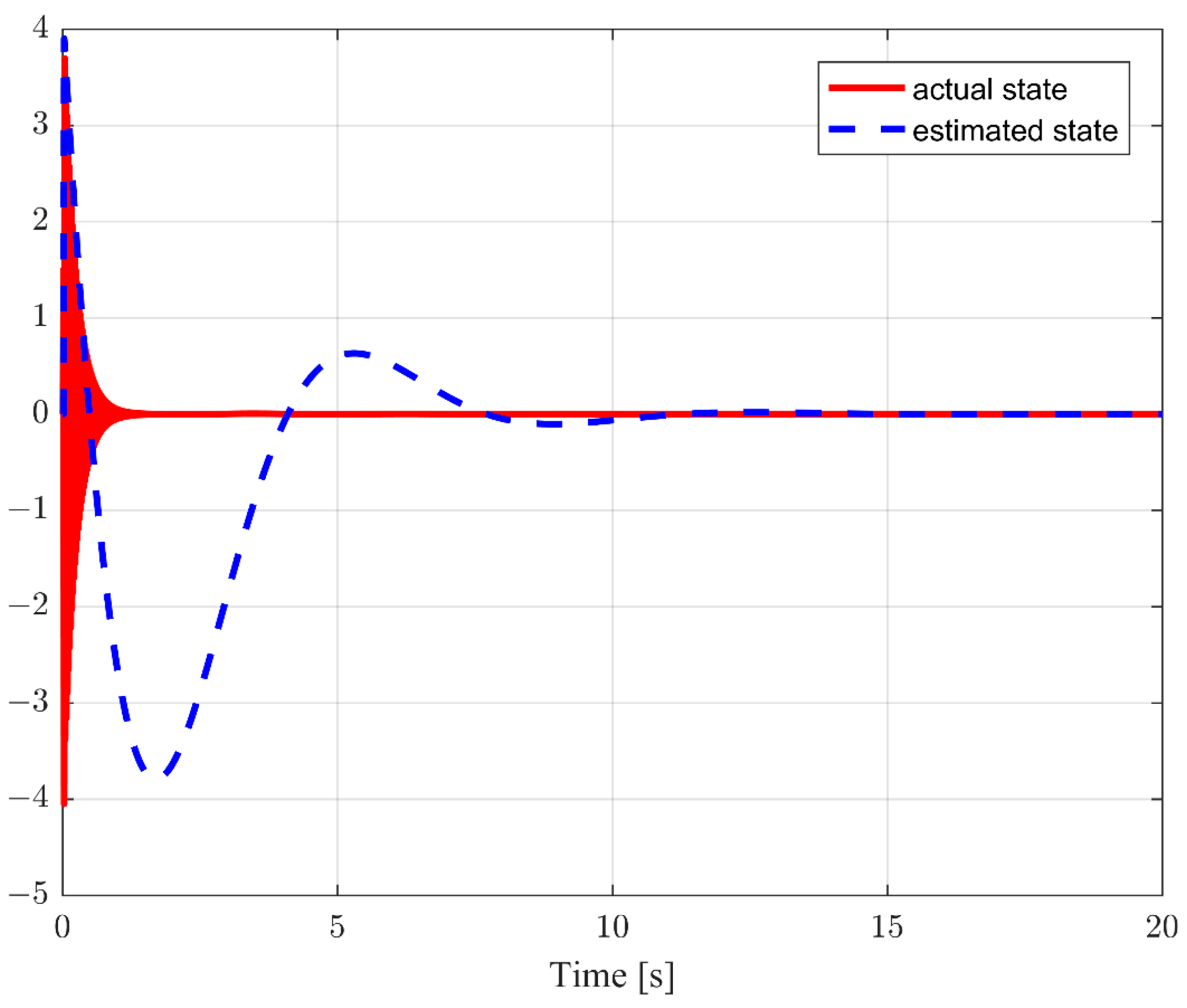
- The works [30,31,32] assumed that all system states can be accurately obtained through measurements, and their studies were carried out on this basis. However, in practical engineering, some control signals are difficult to detect directly due to the influence of noise. This may lead to inaccurate system control. To overcome this challenge, this paper uses high-gain observers to estimate the boundary states of the system.
- (2)
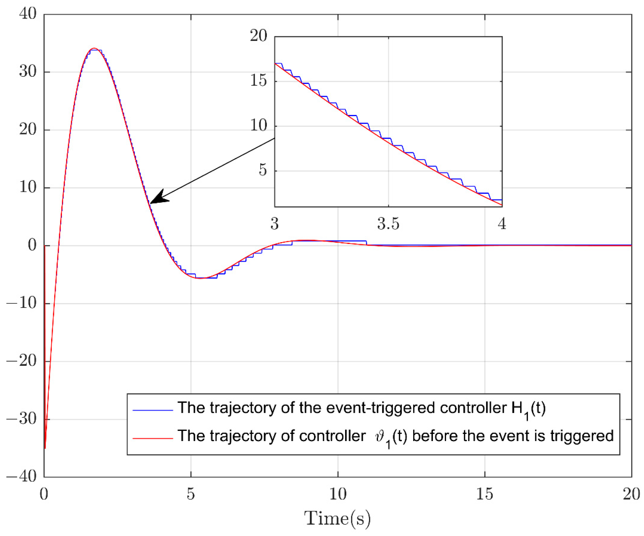
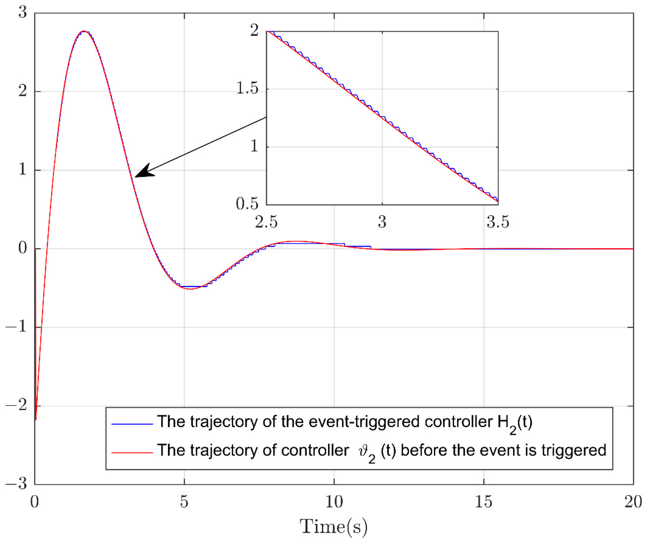
- ET control can effectively lighten the computational burden and communication requirements of the controller and improve the energy efficiency of the system. This control method has received extensive attention and was utilized in [33,34]. However, although ET control has made remarkable achievements in many fields, there is still a lack of relevant research in the specific field of FWRAs. How to optimize the control performance of FWRAs and reduce their resource consumption through an ET mechanism has become a key problem to solve urgently. Therefore, this paper proposes output feedback ET controllers with which the vibrations of an FWRA are effectively suppressed, while communication resources are saved and the communication burden is reduced.
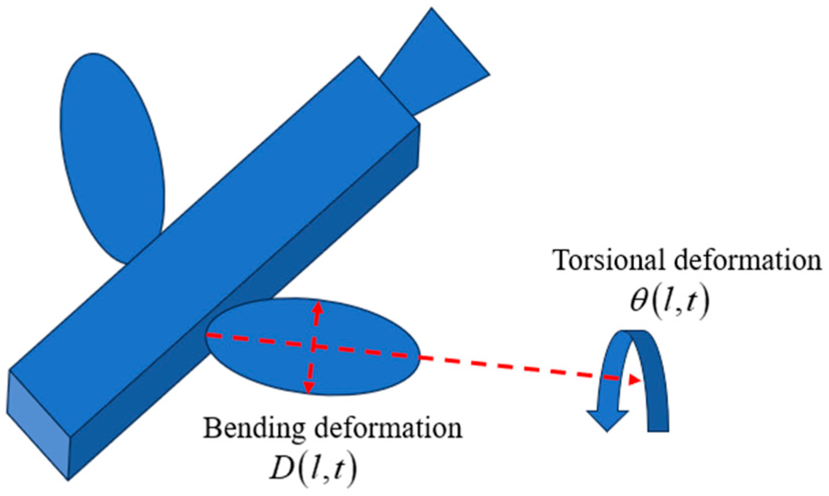
2. System Modeling and Preliminaries
3. Controller Design and Stability Analysis
3.1. Design of the Output Feedback ET Controllers
3.2. The Stability Analysis
- (1)
- All of the signals are bounded;
- (2)
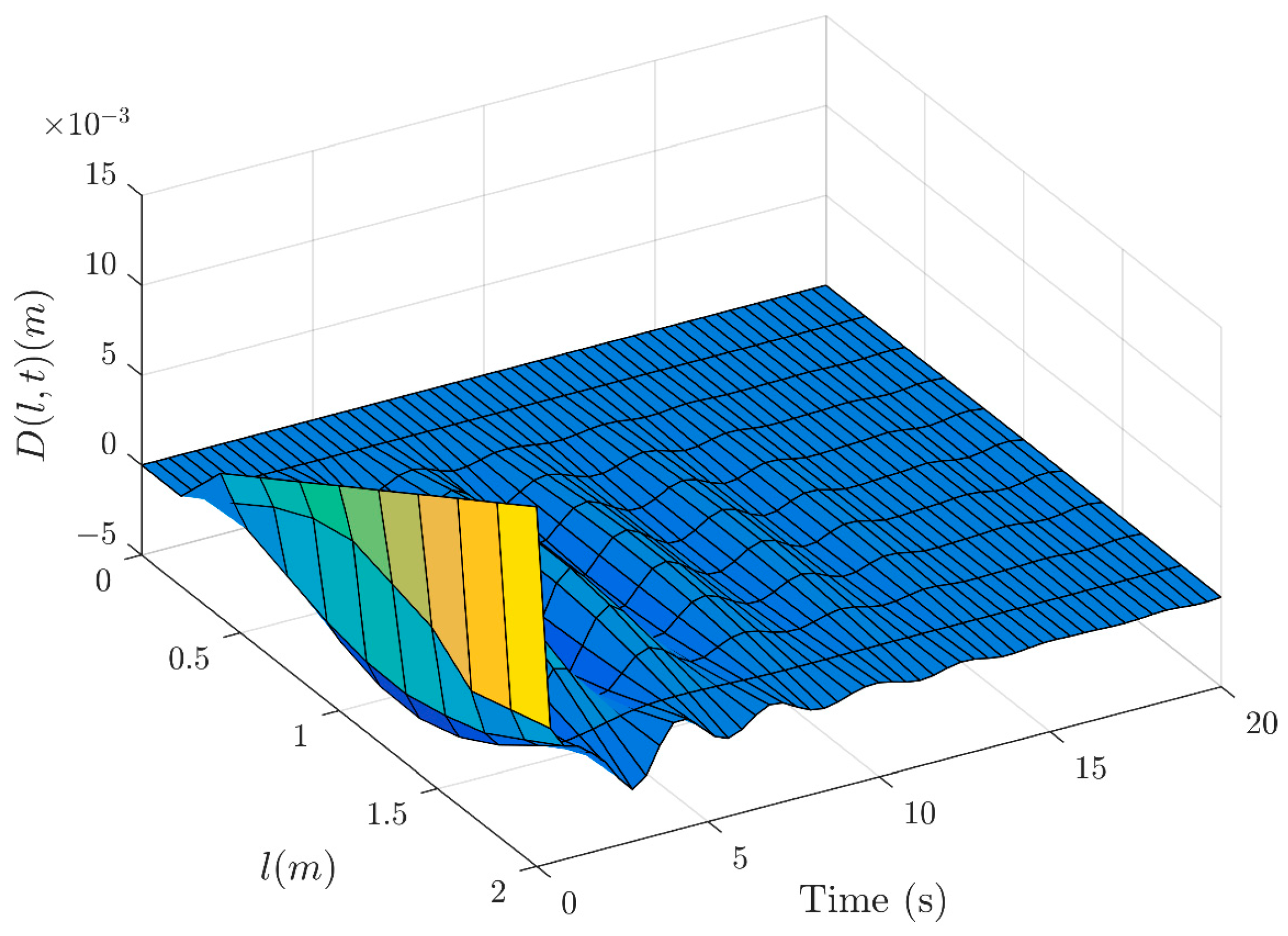
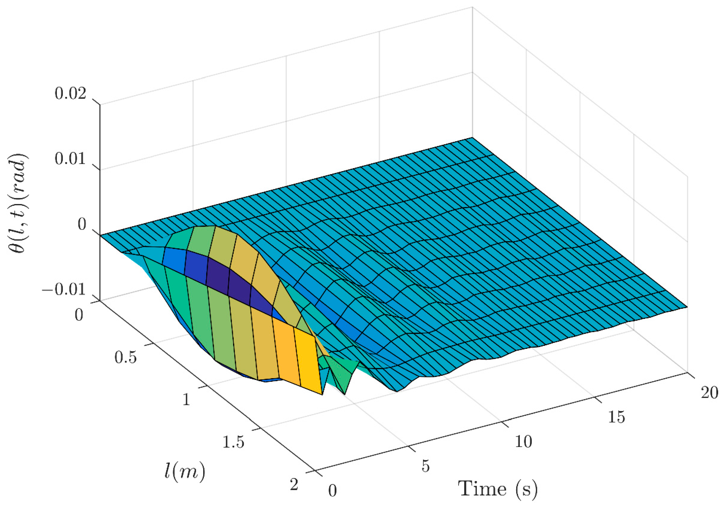
- The vibrations of bending deformation and torsional deformation in the FWRA are effectively suppressed;
- (3)
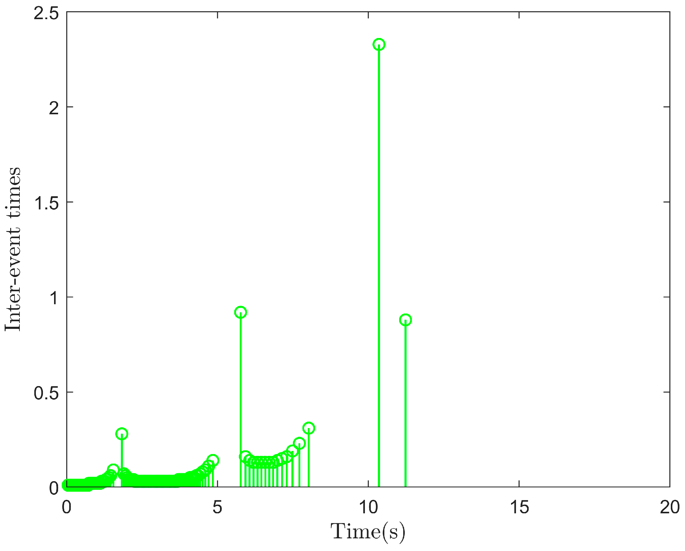
- The Zeno phenomenon is avoided.
4. The Simulation Example
5. Conclusions
Author Contributions
Funding
Data Availability Statement
Conflicts of Interest
References
- Pan, E.; Liang, X.; Xu, W.F. Development of vision stabilizing system for a large-scale flapping-wing robotic bird. IEEE Sens. J. 2020, 20, 8017–8028. [Google Scholar] [CrossRef]
- He, W.; Mu, X.X.; Chen, Y.N.; He, X.Y.; Yao, Y. Modeling and vibration control of the flapping-wing robotic aircraft with output constraint. J. Sound Vib. 2018, 423, 472–483. [Google Scholar] [CrossRef]
- Gao, H.J.; He, W.; Zhang, Y.M.; Sun, C.Y. Adaptive finite-time fault-tolerant control for uncertain flexible flapping wings based on rigid finite element method. IEEE Trans. Cybern. 2021, 52, 9036–9047. [Google Scholar] [CrossRef]
- Pan, E.; Xu, H.; Yuan, H.; Peng, J.Q.; Xu, W.F. HIT-Hawk and HIT-Phoenix: Two kinds of flapping-wing flying robotic birds with wingspans beyond 2 meters. Biomim. Intell. Robot. 2021, 1, 100002. [Google Scholar] [CrossRef]
- He, W.; Mu, X.X.; Zhang, L.; Zou, Y. Modeling and trajectory tracking control for flapping-wing micro aerial vehicles. IEEE/CAA J. Autom. Sin. 2021, 8, 148–156. [Google Scholar] [CrossRef]
- He, W.; Meng, T.T.; He, X.Y.; Sun, C.Y. Iterative learning control for a flapping wing micro aerial vehicle under distributed disturbances. IEEE Trans. Cybern. 2019, 49, 1524–1535. [Google Scholar] [CrossRef] [PubMed]
- Xu, W.F.; Pan, E.; Liu, J.T.; Li, Y.H.; Yuan, H. Flight control of a large-scale flapping-wing flying robotic bird: System development and flight experiment. Chin. J. Aeronaut. 2022, 35, 235–249. [Google Scholar] [CrossRef]
- He, W.; Yan, Z.C.; Sun, C.Y.; Chen, Y.N. Adaptive neural network control of a flapping wing micro aerial vehicle with disturbance observer. IEEE Trans. Cybern. 2017, 47, 3452–3465. [Google Scholar] [CrossRef]
- Zhao, W.; Liu, Y.; Yao, X.Q. Adaptive fuzzy containment and vibration control for multiple flexible manipulators with model uncertainties. IEEE Trans. Fuzzy Syst. 2023, 31, 1315–1326. [Google Scholar] [CrossRef]
- Zhao, Z.J.; Tan, Z.F.; Liu, Z.J.; Efe, M.O.; Ahn, C.K. Adaptive inverse compensation fault-tolerant control for a flexible manipulator with unknown dead-zone and actuator faults. IEEE Trans. Ind. Electron. 2023, 70, 12698–12707. [Google Scholar] [CrossRef]
- Yao, X.Q.; Liu, Y.; Zhao, W. Adaptive boundary vibration control and angle tracking consensus of networked flexible Timoshenko manipulator systems. IEEE Trans. Syst. Man Cybern. Syst. 2023, 53, 2949–2960. [Google Scholar] [CrossRef]
- Jin, F.F.; Guo, B.Z. Lyapunov approach to output feedback stabilization for the Euler–Bernoulli beam equation with boundary input disturbance. Automatica 2015, 52, 95–102. [Google Scholar] [CrossRef]
- Ji, N.; Liu, J.K. Quantized time-varying fault-tolerant control for a three-dimensional Euler–Bernoulli beam with unknown control directions. IEEE Trans. Autom. Sci. Eng. 2023, 21, 6528–6539. [Google Scholar] [CrossRef]
- Cheng, Y.; Wu, Y.; Guo, B.Z. Boundary stability criterion for a nonlinear axially moving beam. IEEE Trans. Autom. Control 2022, 67, 5714–5729. [Google Scholar] [CrossRef]
- Liu, Y.; Wang, Y.N.; Feng, Y.H.; Wu, Y.L. Neural network-based adaptive boundary control of a flexible riser with input dead zone and output constraint. IEEE Trans. Cybern. 2022, 52, 13120–13128. [Google Scholar] [CrossRef]
- He, W.; Sun, C.; Ge, S.Z.S. Top tension control of a flexible marine riser by using integral-barrier Lyapunov function. IEEE/ASME Trans. Mechatron. 2015, 20, 497–505. [Google Scholar] [CrossRef]
- Zhao, Z.J.; He, X.Y.; Ren, Z.G.; Wen, G.L. Boundary adaptive robust control of a flexible riser system with input nonlinearities. IEEE Trans. Syst. Man Cybern. Syst. 2019, 49, 1971–1980. [Google Scholar] [CrossRef]
- Xing, X.Y.; Liu, J.K. PDE modelling and vibration control of overhead crane bridge with unknown control directions and parametric uncertainties. IET Control Theory Appl. 2020, 14, 116–126. [Google Scholar] [CrossRef]
- Li, L.; Liu, J.K. Consensus tracking control and vibration suppression for nonlinear mobile flexible manipulator multi-agent systems based on PDE model. Nonlinear Dyn. 2023, 111, 3345–3359. [Google Scholar] [CrossRef]
- Zhao, Z.J.; Liu, Y.; Luo, F. Output feedback boundary control of an axially moving system with input saturation constraint. ISA Trans. 2017, 68, 22–32. [Google Scholar] [CrossRef]
- Minowa, A.; Toda, M. A high-gain observer-based approach to robust motion control of towed underwater vehicles. IEEE J. Ocean. Eng. 2019, 44, 997–1010. [Google Scholar] [CrossRef]
- Zhang, S.; Liu, R.; Peng, K.X.; He, W. Boundary output feedback control for a flexible two-link manipulator system with high-gain observers. IEEE Trans. Control Syst. Technol. 2021, 29, 835–840. [Google Scholar] [CrossRef]
- Lou, D.K.; Zhang, D.; Liang, H.G. An improved high-gain observer design for flexible needle steering. IEEE Trans. Circuits Syst. II Express Briefs 2023, 70, 3489–3493. [Google Scholar] [CrossRef]
- Lin, N.; Ling, Q. Dynamic periodic event-triggered consensus protocols for linear multiagent systems with network delay. IEEE Syst. J. 2023, 17, 1204–1215. [Google Scholar] [CrossRef]
- Mu, R.; Wei, A.R.; Li, H.T.; Zhang, X.F.; Qi, Y.N. Bipartite output consensus for heterogeneous multi-agent systems with observer-based adaptive event-triggered strategy. IEEE Syst. J. 2023, 17, 6011–6021. [Google Scholar] [CrossRef]
- Song, X.N.; Zhang, Q.Y.; Song, S.; Ahn, C.K. Event-triggered underactuated control for networked coupled PDE-ODE systems with singular perturbations. IEEE Syst. J. 2023, 17, 4474–4484. [Google Scholar] [CrossRef]
- Zhao, X.N.; Zhang, S.; Liu, Z.L.; Wang, J.Y.; Gao, H.B. Adaptive event-triggered boundary control for a flexible manipulator with input quantization. IEEE/ASME Trans. Mechatron. 2022, 27, 3706–3716. [Google Scholar] [CrossRef]
- Wang, J.; Krstic, M. Event-triggered output-feedback backstepping control of sandwich hyperbolic PDE systems. IEEE Trans. Autom. Control 2022, 67, 220–235. [Google Scholar] [CrossRef]
- Cai, G.; Wu, T.; Hao, M.; Liu, H.; Zhou, B. Dynamic event-triggered gain-scheduled H∞ control for a polytopic LPV model of morphing aircraft. IEEE Trans. Aerosp. Electron. Syst. 2025, 61, 93–106. [Google Scholar] [CrossRef]
- Tang, L.; Wang, F. Improving health operation of flapping-wing robotic aircraft systems using event-triggered vibration control technology. IEEE Trans. Consum. Electron. 2025. [Google Scholar] [CrossRef]
- Long, H.; Zhang, P.; Guo, T.; Zhao, J. Fixed-time adaptive fuzzy fault-tolerant control of flapping wing MAVs with wing damage. IEEE Trans. Aerosp. Electron. Syst. 2024, 60, 6594–6607. [Google Scholar] [CrossRef]
- Meng, T.; Guo, B.Z.; Huang, H.; He, W. Iterative learning control for a flexible wing system under iteration-varying disturbances and references. IEEE Trans. Aerosp. Electron. Syst. 2024, 60, 5973–5981. [Google Scholar] [CrossRef]
- Tang, L.; Li, Y.; Liu, Y.J. Adaptive event-triggered vibration control for crane bridge system with trolley. IEEE Trans. Instrum. Meas. 2023, 72, 5504010. [Google Scholar] [CrossRef]
- Gao, S.Q.; Liu, J.K. Event-triggered vibration control for a class of flexible mechanical systems with bending deformation and torsion deformation based on PDE model. Mech. Syst. Signal Process. 2022, 164, 108255. [Google Scholar] [CrossRef]
- Zhao, W.; Sun, H.; Zhao, Z.; Liu, Y. Adaptive fault-tolerant control for flexible manipulators multiagent systems with unknown dead-zones under switching topology. IEEE Trans. Syst. Man Cybern. Syst. 2024, 54, 5412–5421. [Google Scholar] [CrossRef]


| Controller | ET Controllers | Time-Triggered Controllers | ||
|---|---|---|---|---|
| Number of triggers | 140 | 194 | 1998 | 1998 |
Disclaimer/Publisher’s Note: The statements, opinions and data contained in all publications are solely those of the individual author(s) and contributor(s) and not of MDPI and/or the editor(s). MDPI and/or the editor(s) disclaim responsibility for any injury to people or property resulting from any ideas, methods, instructions or products referred to in the content. |
© 2025 by the authors. Licensee MDPI, Basel, Switzerland. This article is an open access article distributed under the terms and conditions of the Creative Commons Attribution (CC BY) license (https://creativecommons.org/licenses/by/4.0/).
Share and Cite
Xiao, C.; Tang, L.; Wang, F.; You, S.; Xu, H.; Chen, M.; Lu, Z. Event-Triggered Control for Flapping-Wing Robot Aircraft System Based on High-Gain Observers. Actuators 2025, 14, 190. https://doi.org/10.3390/act14040190
Xiao C, Tang L, Wang F, You S, Xu H, Chen M, Lu Z. Event-Triggered Control for Flapping-Wing Robot Aircraft System Based on High-Gain Observers. Actuators. 2025; 14(4):190. https://doi.org/10.3390/act14040190
Chicago/Turabian StyleXiao, Chenxu, Li Tang, Fei Wang, Sheng You, Hao Xu, Mingchuang Chen, and Zhiyuan Lu. 2025. "Event-Triggered Control for Flapping-Wing Robot Aircraft System Based on High-Gain Observers" Actuators 14, no. 4: 190. https://doi.org/10.3390/act14040190
APA StyleXiao, C., Tang, L., Wang, F., You, S., Xu, H., Chen, M., & Lu, Z. (2025). Event-Triggered Control for Flapping-Wing Robot Aircraft System Based on High-Gain Observers. Actuators, 14(4), 190. https://doi.org/10.3390/act14040190