Article

A Novel Cycloid Tooth Profile for Harmonic Drive with Fully Conjugate Features

1
School of Mechanical & Automotive Engineering, South China University of Technology, Guangzhou 510641, China
2
School of Mechanical Engineering, Tiangong University, Tianjin 300387, China
3
School of Aeronautics and Astronautics, Tiangong University, Tianjin 300387, China
*
Author to whom correspondence should be addressed.
Actuators 2025, 14(4), 187; https://doi.org/10.3390/act14040187
Submission received: 16 March 2025 / Revised: 9 April 2025 / Accepted: 10 April 2025 / Published: 11 April 2025
(This article belongs to the Section Precision Actuators)

Abstract

:
A harmonic drive (HD) is a precision reduction device widely utilized in the core joints of high-end equipment such as spacecraft and robots. The design of an excellent tooth profile is the core challenge related to the performance of HD. This investigation aims to propose a design method of a fully conjugated cycloid tooth profile (CTP) for HD. Firstly, the rationality of CTP use for HD is analyzed, and the cycloidal characteristics of the tooth trajectory are studied by use of canonical warping distance. Then, initial CTP equations are constructed, adopting the trajectory mapping results. Presetting the addendum CTP of circular spline, the conjugate CTP of flexspline is then designed using the envelope method. Subsequently, the envelope of the designed flexspline addendum is used to reverse-design the circular spline dedendum. The backlash is calculated to evaluate the CTPs designed with different radial displacement coefficients. Research shows that the tooth trajectory has cycloidal characteristics; therefore, the HDs that use CTP can realize a fully conjugate engagement. Moreover, the variable control parameters enable the proposed CTP expression to have excellent fitting characteristics, resulting in small and uniform mesh backlash distribution. The CTP is expected to become one of the ideal tooth profiles of HD.

1. Introduction

A harmonic drive (HD) is a lightweight transmission mechanism that aligns with the stringent requirements of spacecraft reducers—namely, light weight, compact dimensions, and exceptional precision—while simultaneously offering robust load-bearing capabilities. Consequently, HD has found extensive applications across diverse fields, including robotics, aerospace systems, and medical devices [1,2,3]. A central challenge in HD research stems from the fluctuating deformations of the flexspline (FS), which has rendered the meshing theory and tooth profile (TP) design enduringly complex and pivotal areas of investigation within this domain.
Numerous research methodologies have been developed to investigate the meshing theory of HD, with the envelope method and the kinematic method being the most widely adopted. Shen et al. [4] established a generalized formula for calculating the conjugate TP of HDs using the envelope method. Building on this, Chen et al. [5] introduced a precise envelope algorithm that accounts for the elastic deformation of the FS. Recognizing the influence of the wave generator (WG) shape on the relative motion between the FS and the circular spline (CS) [6], Yang et al. [7] developed an exact solution method for determining the conjugate TP based on cam profiles. Further advancing the field, Dong et al. [8] conceptualized the FS and WG as a cam-follower mechanism, providing a rigorous analysis and detailed description of the planar kinematic model of HDs. In a comparative study, Wang et al. [9] evaluated the kinematic method and the envelope method through the design outcomes of a double circular arc TP, concluding that the envelope method offers superior accuracy.
In the context of TP design, HD initially employed a straight TP to achieve surface-to-surface contact between tooth surfaces. However, this approach failed to account for the circumferential displacement and normal deflection of the tooth rim. Consequently, the technologically mature, involute TP was later widely adopted in HDs. Maiti [10] demonstrated that an unmodified involute TP could function effectively through the strategic design of the cam. The application and refinement of involute TPs in HDs have been extensively studied [11,12]. Nevertheless, involute HDs exhibit poor conjugate characteristics, relying primarily on cusp meshing at the tooth tips to achieve multi-tooth engagement [4]. This cusp meshing condition, however, tends to disrupt the lubricant film and accelerate tooth wear, rendering the involute profile suboptimal for HD applications. Additionally, while the involute TP of the CS as an internal gear is concave, Ivanov [13] proposed that the CS TP should be convex based on an analysis of the motion characteristics of the FS teeth. This insight led Ivanov to pioneer the double-arc TP for HDs. Since its introduction, the double circular arc TP has become the dominant approach in HD profile design [14,15]. The double circular arc TP not only significantly enhances the conjugate existence interval of HDs by incorporating a convex TP for the CS [16,17] but also further improves meshing performance by synchronizing the convex and concave segments of the CS through the utilization of double-conjugate characteristics [18,19].
The distinctive characteristics of the double-arc TP have inspired the development and design of novel TPs for HD. Ishikawa et al. [20] introduced an S-shaped TP directly derived from the halved mapping of the tooth trajectory using the rack approximation method. This innovative profile incorporates both concave and convex segments. Through appropriate TP modifications [21], which address the interference caused by the normal deflection angle of the FS, the S-shaped TP achieves continuous contact with similarly designed profiles. In a comparative study, Wang et al. [22] evaluated the double-arc TP designed via the envelope method and the S-shaped TP developed using the rack approximation method, revealing that the S-shaped profile exhibits smaller and more uniform meshing backlash. As a result, both the double circular arc TP and the S-shaped TP have gained widespread adoption in HD applications.
The studies on the double-arc TP and the S-shaped TP demonstrate that it is both logical and effective to consider the motion characteristics of HD and to design TPs directly based on the motion trajectory of gear teeth. Shen et al. [4] observed that the relative motion trajectory of HD tooth approximates a cycloid. Building on this insight, Le et al. [23] proposed a cycloidal TP (CTP) composed of epicycloid and inner cycloid segments for HDs. Subsequently, the CTP was further refined through the TP angle design [24] to eliminate interference within the backlash [25]. This CTP exhibits theoretical properties akin to those of the double circular arc TP. However, the current CTP is not directly derived from the tooth trajectory, suggesting that there remains significant potential for further optimization and improvement of this profile.
The objective of this paper is to propose a novel construction and design methodology for a CTP tailored for HD, leveraging the combined advantages of trajectory mapping and the envelope method. First, canonical correlation analysis is employed to validate the cycloidal characteristics of the tooth trajectory, followed by the formulation of a CTP equation for HD with variable coefficients. While this equation is inspired by the trajectory mapping method, it is not constrained by its results; instead, the variable coefficients ensure the design flexibility of the CTP. Subsequently, the CTPs of the FS and CS are meticulously designed using the envelope method and the bidirectional conjugate design flow [16].
In addition to the Introduction section, this article is structured as follows. Section 2 analyzes the rationality of the CTP, calculates the HD tooth trajectories, and verifies their cycloidal characteristics. Section 3 constructs the initial cycloidal equations for the TP based on the trajectory mapping relationship and presents the bidirectional conjugate design process for the CTP using the envelope method. Section 4 provides an example of a TP design, discussing the designed CTP in terms of its conjugate characteristics and backlash distribution. Section 5 examines the results of the TP design under varying deformation magnitudes. Finally, Section 6 summarizes the main conclusions of this paper.

2. Rationality Analysis of Cycloid Tooth Profile

When the WG is installed, the FS undergoes deformation, forming a differential meshing relationship with the CS. As the WG rotates, a periodic “meshing in–meshing out” motion is established between the teeth of the FS and CS. This section calculates the tooth trajectory of the HD, extracts the coordinates of several points on the trajectory as the query array s1, and compares it with a reference array s2 extracted from a general cycloid. By employing canonical correlation analysis, the similarity between the tooth trajectory and the general cycloid is verified using the canonical time warping distance. Furthermore, a cycloidal expression for the tooth trajectory is constructed, thereby validating the rationality of applying a CTP to HDs based on tooth trajectory mapping.

2.1. Calculation of Tooth Trajectory

As illustrated in Figure 1, the neutral circle of the FS with radius rm undergoes elliptical deformation under the influence of the WG. The coordinate system S0-OXY is fixed to the WG, with point O at the center of rotation and the Y-axis aligned with the major axis of the WG. The coordinate system S1-O1X1Y1 is fixed to the FS tooth, with point O1 located on the neutral line of the FS and the Y1-axis aligned with the symmetry line of the tooth (normal at point O1). ρ is the polar radius of point O1. The coordinate system S2-OX2Y2 is fixed to the CS tooth, with the Y2-axis aligned with the symmetry line of the tooth space. The angle φ represents the initial position of point O1 relative to the Y-axis, while φ1 denotes the angle between their new positions after deformation.
Assuming negligible elongation of the FS under internal deformation forces [26], the midline non-elongation assumption is approximately satisfied. Consequently, the angles φ and φ1 are related as follows:
φ = 1 r m 0 ϕ ρ 2 + ρ 2 d φ 1 ,
here, the integral limit ϕ is equal to the related angle φ1 of the polar radius ρ.
φ2 denotes the angle between the symmetry line of the CS tooth space and the Y-axis.
φ 2 = φ z 1 / z 2 ,
here, z1 and z2 denote the tooth number of FS and CS, respectively. The angle between the FS tooth positioning point O1 and the symmetry line of the corresponding CS tooth space is as follows:
θ γ = φ 1 φ z 1 / z 2 ,
Additionally, θμ represents the deflection angle of the normal to the neutral line of the deformed FS, i.e., the angle between the tooth symmetry line and the polar diameter ρ. According to the exact algorithm [5],
θ μ = arctan ρ / ρ ,
θp represents the angle between the symmetry line of the CS tooth space and the symmetry line of the FS tooth, which form the corresponding meshing tooth pair.
θ p = θ μ + θ γ ,
The deflection angle θμ influences the trajectory of any point on the FS’s TP but does not affect the trajectory of the positioning point O1, which lies on the neutral line. Therefore, to simplify the problem, the trajectory of point O1 is taken as the tooth trajectory to be studied. As illustrated in Figure 1, when the FS undergoes deformation, O1 is allocated a polar diameter ρ in the coordinate system S0. Consequently, the coordinates of point O1 in the coordinate system S2 are as follows:
x 2 O 1 = ρ sin θ γ y 2 O 1 = ρ cos θ γ ,
here, both ρ(φ1) and θγ are functions of the polar angle φ1, indicating that when φ1 varies between 0 and π/2, the tooth trajectory expressed in coordinate system S2 can be obtained using Equation (6). From Equation (6), it is evident that the tooth trajectory ultimately depends on the deformation shape of the neutral line of the FS, which is determined by ρ(φ1).

2.2. Cycloid Characteristic of Tooth Trajectory

Analytically deriving formulas to demonstrate the similarity between the tooth trajectory and a general cycloid is highly challenging. Instead, a discrete point similarity analysis method can be effectively employed to study the cycloidal characteristics of the tooth movement locus. Canonical correlation analysis (CCA), a widely recognized method for identifying correlations between two sets of multidimensional variables [27], serves as a suitable tool for this purpose. During the analysis, the correlation variables s1α and s2β are constructed by introducing projection transformation matrices α and β for any sequence s1 and s2 and then used to determine the correlation coefficients, with their corresponding transformation matrices α and β adhering to the principle of maximum correlation. In CCA, the correspondence of elements in s1 and s2 follows the original element order.
Therefore, relying solely on canonical CCA is insufficient to accurately judge the similarity between two curves with distorted shapes. To address this limitation, canonical time warping (CTW) [28] is introduced. CTW iteratively adjusts the correspondence between the elements of sequences s1 and s2 and performs the projection transformations α and β to minimize the residual sum of squares (RSS) of the two sequences. The minimum RSS obtained for sequences s1 and s2 through two levels of optimization—CCA and CTW—is defined as the canonical warping distance (CWD).
J s = i = 1 k α i s 1 [ n i ] β i s 2 [ m i ] 2 ,
here, ni and mi represent the correspondence of sequences s1 and s2 after CTW, respectively; s1[ni] and s2[mi] denote the corresponding elements; αi and βi are the elements in the projection matrices, and k is the elements number of s1[ni] and s2[mi]. CTW demonstrates superior robustness to spatial transformations, enabling the CWD to accurately capture the similarity between two sequences, even in the presence of relative displacement, rotation, and scaling in space.
An arbitrary model with the parameters listed in Table 1 is established for the tooth trajectory calculation. The maximum radial displacement coefficient w0* in Table 1 is defined as the ratio of the designed maximum radial displacement w0 of the FS to the modulus m, i.e., w0* = w0/m.
Taking the deformation of the FS under the action of the elliptical WG as an example, the polar coordinate expression of the neutral line of the FS after deformation is as follows:
ρ = ρ a ρ b ρ a 2 sin 2 φ 1 + ρ b 2 cos 2 φ 1 ,
here,
ρ a = r m + m w 0 * ,
ρ b = 1 / 9 ( 12 r m 7 ρ a ) + 4 ρ a ( 3 r m 2 ρ a ) ,
represent the polar diameters of the major axis and the minor axis of the FS’s neutral line, respectively. The tooth trajectory of the model specified in Table 1 is calculated for φ1, ranging from 0 to π/2 using Equation (6). The coordinates of 90 points on the trajectory are extracted to form the query sequence s1.
The general expression of the cycloid formed by the trajectory of a point fixed on a circle as the circle rolls along a straight line is obtained using the following equation [29]:
x t = r g t sin t y t = r g 1 cos t ,
Let the radius of the rolling circle be rg = 1 mm, the coordinates of 90 points on the cycloid are calculated for t, ranging from 0 to π, by using Equation (9) to form the reference sequence s2. The tooth trajectory sequence s1 and the general cycloid sequence s2 are illustrated in Figure 2. Perform the CWD calculation between sequences s1 and s2 in Mathematica. The result is as follows:
Js = 2.61 × 10⁻⁵,
Js is very close to zero, indicating that the tooth trajectory exhibits a high degree of similarity to the cycloid. This result demonstrates that the correlation between the tooth trajectory and the general cycloid is accurately identified after CTW, despite significant differences in the positions and angles of the tooth trajectory and the general cycloid, as shown in Figure 2.
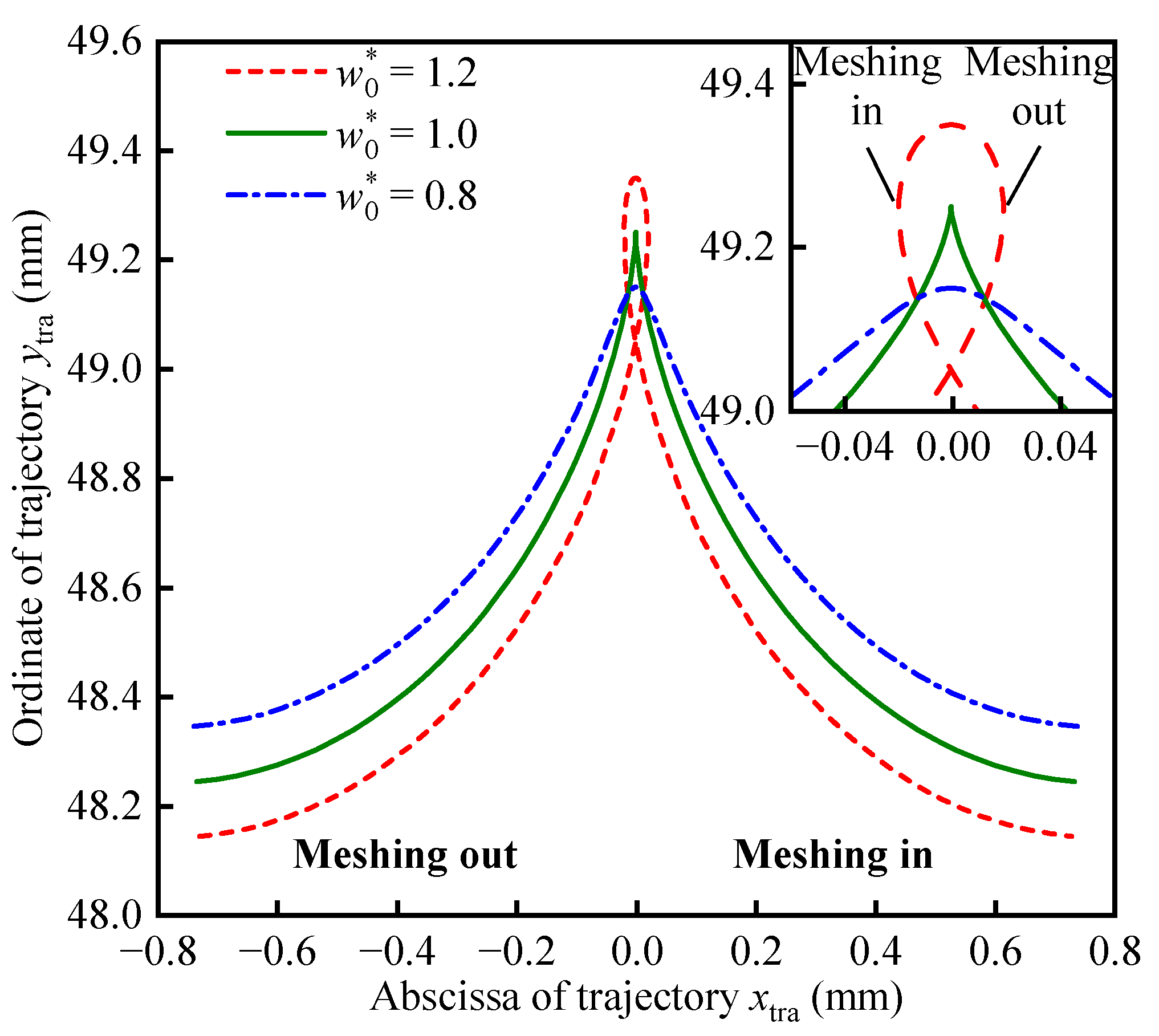
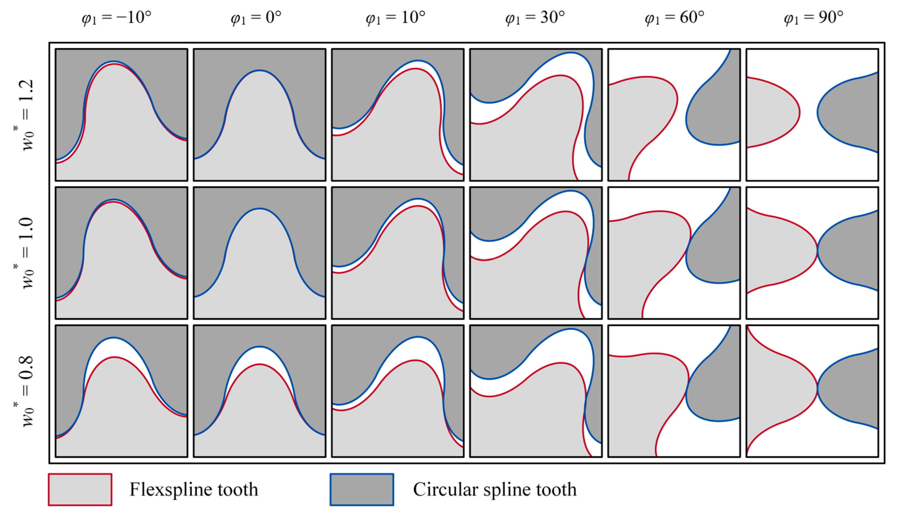
Therefore, the tooth trajectory exhibits cycloid characteristics. While the tooth trajectory can display different characteristics (see Figure 8 for details when w0* = 1.2 and w0* = 0.8), both prolate cycloids and curtate cycloids can effectively match these variations. However, the standard cycloid (Equation (9)), which aligns with the tooth trajectory when w0* = 1.0, is the most convenient for curve mapping calculations.

2.3. X-Halved Cycloid Tooth Trajectory

Let the radius of the rolling circle in Equation (9) be equal to the modulus of the HD, i.e., rg = m. A cycloid with the x-coordinate compressed by half is constructed as follows:
x t = m t sin t / 2 y t = m 1 cos t ,
The geometry, slope, and curvature of the tooth trajectory and the cycloid expressed in Equation (10) are calculated and illustrated in Figure 3.
Figure 3a illustrates the trajectory (xtra, ytra) of a complete meshing process of the FS’s tooth as φ1 varies from 0 to π/2, alongside the cycloid (xcyc, ycyc), with its x-coordinate halved as t changes from 0 to π. Although the ordinate ranges of the two curves are not consistent, the geometric shape of the tooth trajectory aligns precisely with the cycloid in which the x-coordinate is halved. Furthermore, as shown in Figure 3b,c, the slope and curvature of the tooth trajectory and the cycloid are identical.
The results in Figure 3 demonstrate that the tooth trajectory can be approximately expressed by a cycloid with its x-coordinate halved. Since the tooth trajectory is a cycloid, the TP obtained using the halved mapping of the trajectory can also be represented by a cycloid. Therefore, the application of a CTP in HD is justified. Although these results are derived from the trajectory of a specific model under the influence of an elliptical WG, they also reflect, to a certain extent, the common characteristics of the tooth trajectory in harmonic drives.

3. Method of Cycloid Tooth Profile Design

Directly constructing the meshing TPs of the CS and FS based on the trajectory mapping curve represents a fundamentally sound approach. However, to address potential TP interference caused by the normal rotation of the FS, modifications to the TPs are essential [21]. To meet the requirements of precise conjugation, the TP design can be refined using the envelope method. Additionally, the double-conjugate phenomenon in HD [15,18] can be leveraged to form viable conjugate TPs through practical design. The bidirectional conjugate design process [16] further enhances this by maximizing the double-conjugation effect between meshing tooth pairs. In this section, the addendum profile of the CS is selected as the initial TP, and its CTP equation is formulated based on cycloid mapping. Subsequently, the complete TPs of the CS and FS are achieved through the bidirectional conjugate design process.

3.1. Construction of Initial Cycloid Tooth Profile

As demonstrated in Section 2, the tooth trajectory can be approximated using the cycloid expressed in Equation (10). Consequently, the initial cycloid is constructed by halving the radius of the rolling circle in Equation (10) (i.e., rg = m/2) as follows:
x d = m t sin t / 4 y d = m 1 + cos t / 2 ,
Point symmetry of Equation (11) about the point (0, 0) is as follows:
x u = m t sin t / 4 y u = m 1 + cos t / 2 ,
In the subsequent description, the cycloid expressed in Equation (11) is referred to as the D-cycloid, and the cycloid expressed in Equation (12) is referred to as the U-cycloid. According to the FS tooth coordinate system S1 and the CS tooth coordinate system S2 shown in Figure 1, Equations (11) and (12) can be transformed to represent the TPs of the FS and CS, respectively.
Research on the double-conjugation phenomenon [15,18] has demonstrated that the conjugate result of a convex TP is the primary consideration in TP design. Therefore, the convex TP of either the FS’s tooth addendum or the CS’s tooth addendum can be selected as the initial TP. In this case, the addendum TP of the CS is chosen as the initial TP. According to the coordinate system S2 in Figure 1 and the D-cycloid equation expressed in Equation (11), the initial CTP {xd2(t), yd2(t)} of the CS’s tooth addendum has the following relationship:
x d 2 y d 2 = A d 2 x d y d + B d 2 ,
here,
A d 2 = a x d 2 a r d 2 0 0 a y d 2 a r d 2 ,   B d 2 = e t 2 / 2 + b d 2 R a 2
Ad2 is the scaling coefficients matrix of the D-cycloid, where axd2 is the x-scaling coefficient, ayd2 is the y-scaling coefficient, and ard2 is the scaling coefficient of the rolling circle radius; Bd2 is the coordinate translation matrix of the initial cycloid (Equation (11)) when expressing the addendum profile of CS in coordinate system S2; et2 is the width of the tooth space on the reference circle of CS, bd2 is the x-translation coefficient, and Ra2 is the addendum circle radius of CS. These coefficients allow for the adjustment of the initial cycloid from multiple perspectives, significantly enhancing the design flexibility of the cycloid.

3.2. Envelope of Initial Cycloid Tooth Profile

According to Figure 1, the transformation matrix from coordinate system S2 to S1 is as follows:
T 21 = cos θ p sin θ p ρ sin θ μ sin θ p cos θ p ρ cos θ μ 0 0 1 ,
Therefore, the addendum profile of CS shown in Equation (13) is transformed into the coordinate system S1 as follows:
x d 21 y d 21 1 = T 21 x d 2 y d 2 1 ,
here, both xd21 and yd21 are functions with variables t and φ1, i.e., they represent a cluster of curves distributed along φ1. If an envelope curve exists for this curve cluster, the points on the envelope curve satisfy the envelope condition expressed in Equation (15).
x d 21 t y d 21 φ 1 x d 21 φ 1 y d 21 t = 0 ,
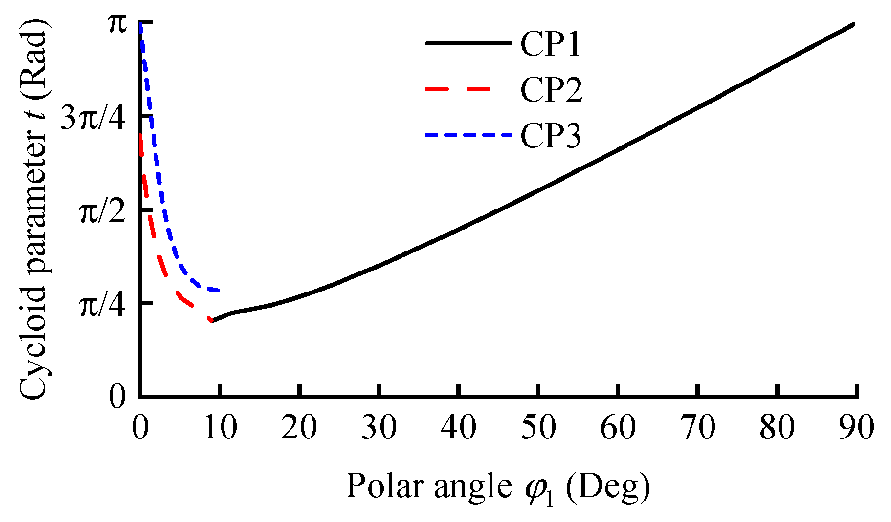
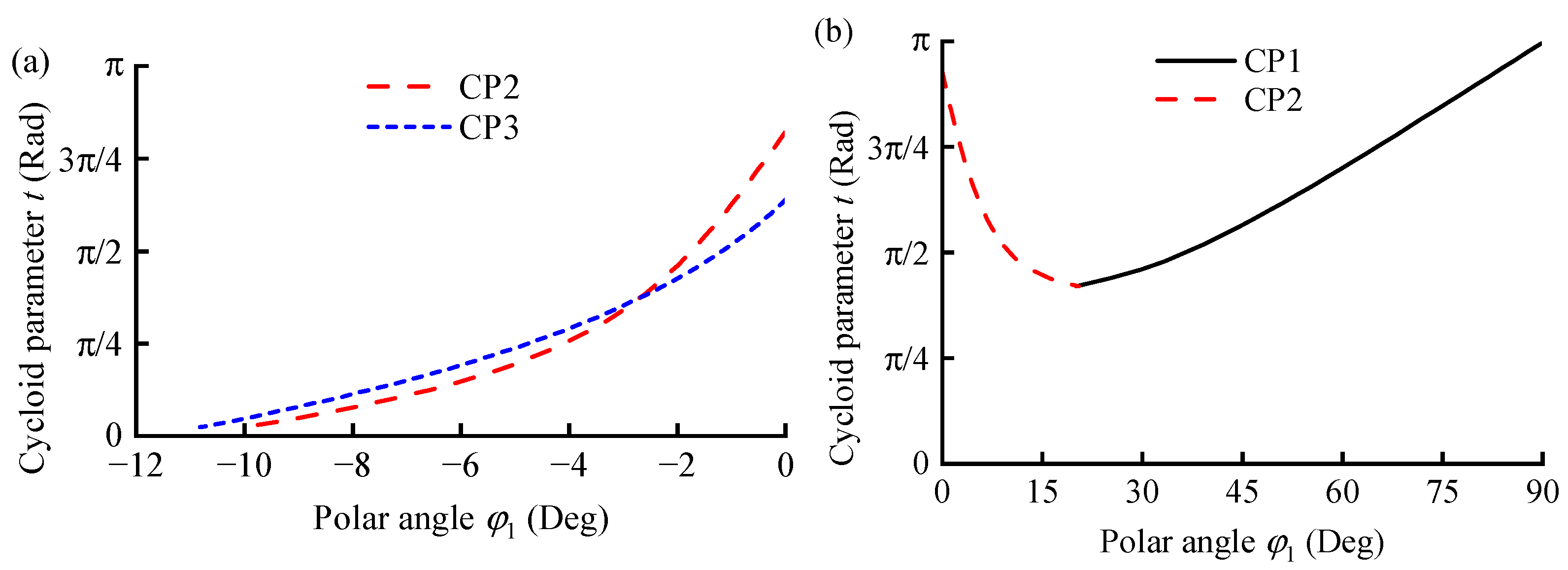
Parameter t of the TP, which satisfies the conjugate condition for any φ1, can be determined using Equation (15). By substituting t and φ1 into Equation (14), the discrete conjugate point of the CS’s addendum can be obtained.

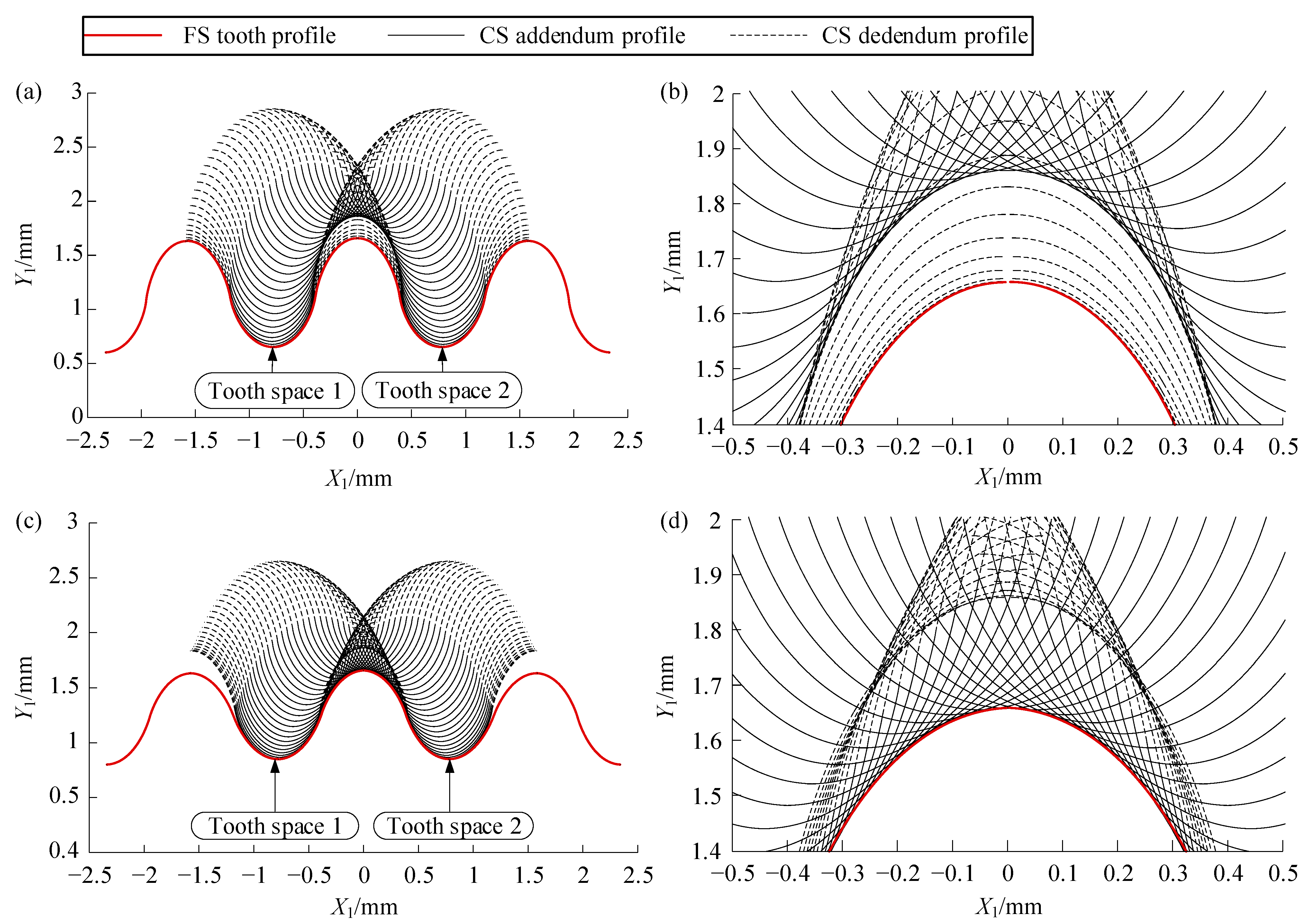
3.3. Cycloid Tooth Profile Design of Flexspline

Preliminary studies on the composite cycloid [24] indicate that the conjugate points of the CTP retain a cycloidal shape and should incorporate a specific TP angle. Trial calculations of the envelope reveal that the conjugate points forming the FS TP not only appear outside the reference circle but also partially distribute within it. Consequently, a CTP with a non-zero TP angle can be constructed, as illustrated in Figure 4.
The TP angle at the joint point of the two cycloids can serve as a design variable, thereby further enhancing the design flexibility of the CTP. In Figure 4, AB represents a U-cycloid, and CD represents a D-cycloid. The tangent angle of AB at point E is α0, and the tangent angle of CD at point F is also α0. By translating AB, the CTP with TP angle α0 can be obtained by smoothly connecting AB and CD at points E and F. The expression {xd1(t), yd1(t)} of FS’s dedendum CTP has the following relationship:
x d 1 y d 1 = A d 1 x d y d + B d 1 ,
here,
A d 1 = a x d 1 a r d 1 0 0 a y d 1 a r d 1 ,   B d 1 = s t 1 / 2 + b d 1 R a 2 ρ a
The initial expression {xu1(t), yu1(t)} of the FS’s addendum CTP has the following relation:
x u 1 y u 1 = A u 1 x u y u + B u 1 ,
here,
A u 1 = a x u 1 a r u 1 0 0 a y u 1 a r u 1 ,   B d 1 = s t 1 / 2 + b d 1 R a 2 ρ a
here, axd1 and axu1 are the x-scaling coefficients; ayd1 and ayu1 are the y-scaling coefficients; ard1 and aru1 are the scaling coefficients of the rolling circle radius; st1 is the tooth thickness of FS on the reference circle (where st1 = et2), and bd1 and bu1 are the x-translation coefficients.
Calculate the first-order derivatives of the U-cycloid and D-cycloid of the FS,
d y u 1 d x u 1 = 2 a y u 1 sin t a x u 1 1 cos t ,   d y d 1 d x d 1 = 2 a y d 1 sin t a x d 1 1 cos t
Let the tooth angle at the connection of the U-cycloid and D-cycloid of the FS be α01. The slope at this position is −cot(α01). Consequently, the tooth parameters at points E and F can be determined as follows:
t E 1 = 2 arccot a x u 1 2 a y u 1 cot α 01 ,   t F 1 = 2 arccot a x d 1 2 a y d 1 cot α 01
The coordinates of points E and F can be determined by substituting tE1 and tF1 into Equations (17) and (16), respectively. By translating the U-cycloid to align point E with point F, the addendum CTP of the FS is expressed as follows:
x u 1 = m [ a x u 1 a r u 1 ( t E 1 t + sin t sin t E 1 ) + a x d 1 a r d 1 ( t F 1 sin t F 1 ) ] / 4 + s 1 / 2 + b d 1 y u 1 = m [ a y u 1 a r u 1 ( cos t E 1 cos t ) + a y d 1 a r d 1 ( 1 + cos t F 1 ) ] / 2 + R a 2 ρ a ,
here, the independent variable t takes values in the range from tE1 to π.
According to Equation (16), the dedendum profile of FS is expressed as follows:
x d 1 = a x d 1 a r d 1 m t sin t / 4 + s 1 / 2 + b d 1 y d 1 = a y d 1 a r d 1 m 1 + cos t / 2 + R a 2 ρ a ,
here, the independent variable t takes values in the range from tF1 to π.
Among the discrete conjugate points of the CS’s addendum, the points located inside the FS’s reference circle are selected for least-squares fitting, using Equation (19) as the target curve, to determine the coefficient matrices Ad1 and Bd1. Subsequently, the points outside the reference circle are fitted using Equation (18) to determine the coefficient matrices Au1, Bu1, and tooth angle α01 of the addendum cycloid of FS. This completes the design of the FS’s CTP.

3.4. Cycloid Tooth Profile Design of Circular Spline

As the FS’s addendum profile design has been completed, its conjugate calculation can be performed to complete the dedendum profile design of CS, which can realize the double-conjugate meshing. This process of the reverse conjugate design of CS’s dedendum by the addendum of FS, which was previously designed by the presetting CS’s addendum, is called a bidirectional conjugate design [16].
Among the discrete conjugate points of the FS’s addendum, the points located inside the CS’s reference circle should align with the initial CTP of the CS addendum, while the points outside the CS’s reference circle can be used to design its dedendum TP. According to Figure 1, the transformation matrix from the coordinate system S1 to S2 is T21−1. According to Equation (13), the CTP of the CS’s dedendum is expressed as follows:
x d 2 = a x d 2 a r d 2 m t sin t / 4 + e 2 / 2 + b d 2 y d 2 = a y d 2 a r d 2 m 1 + cos t / 2 + R a 2 ,
here, the independent variable t takes values ranging from tF2 to π.
The expression of the CS dedendum CTP is as follows:
x u 2 = m [ a x u 2 a r u 2 ( t E 2 t + sin t sin t E 2 ) + a x d 2 a r d 2 ( t F 2 sin t F 2 ) ] / 4 + e 2 / 2 + b d 2 y u 2 = m [ a y u 2 a r u 2 ( cos t E 2 cos t ) + a y d 2 a r d 2 ( 1 + cos t F 2 ) ] / 2 + R a 2 + ρ a ρ b ,
here, the independent variable t takes values ranging from tE2 to π.

4. Case Study

The feasibility of applying the CTP to HD, along with the design methodology and bidirectional conjugate process for the CTP, has been thoroughly discussed in the preceding sections. In this section, a specific example is provided to illustrate the complete design process of the CTPs for both the CS and FS.

4.1. Design Case of Cycloid Tooth Profile

Set the wall thickness of the tooth rim of FS as 1.5 mm, the design maximum radial displacement coefficient w0* = 1.0, and the tooth addendum height coefficient ha* = 1.0. The remaining parameters are referenced from Table 1. According to Equation (8), the diameters of the major and minor axes of the neutral line of the FS are ρa = 49.25 mm and ρb = 48.2474 mm. The radius of the CS’s addendum circle is Ra2 = m(z2/2 − ha*) = 50 mm. The initial parameters are set as follows:
s t 1 = e t 2 = π m / 2 ,   a x d 2 = 1 ,   a y d 2 = 1 ,   a r d 2 = 1 ,   b d 2 = 0
The design is carried out according to the method and process described in Section 3, and the resulting coefficients of the TPs are summarized in Table 2.
By substituting the coefficients shown in Table 2 into Equations (18)–(21), the expression of addendum CTP of CS is as follows:
x d 2 = 0.125 t sin t + 0.3927 y d 2 = 0.25 cos t + 50.25 ,
the expression of dedendum CTP of CS is as follows:
x u 2 = 0.1275 t sin t + 0.407 y u 2 = 0.3233 cos t + 50.6852 ,
the expression of addendum CTP of FS is as follows:
x u 1 = 0.1261 t sin t + 0.4 y u 1 = 0.3093 cos t + 1.4494 ,
and the expression of the dedendum CTP of FS is as follows:
x d 1 = 0.1262 t sin t + 0.3872 y d 1 = 0.2598 cos t + 1.0098

4.2. Case Results

4.2.1. Conjugate Engagement Existence Interval

During the conjugate point calculation process, the conjugate range of the cycloid can also be obtained. The meshing of CS and FS can be divided into three states: the conjugation between CS’s tooth addendum and FS’s tooth addendum (CP1 in Figure 5), the conjugation between CS’s tooth addendum and FS’s tooth dedendum (CP2 in Figure 5), and the conjugation between CS’s tooth dedendum and FS’s tooth addendum (CP3 in Figure 5). There is no meshing relationship between CS’s tooth dedendum and FS’s tooth dedendum.
As illustrated in Figure 5, the addendum of CS and the addendum of FS mesh conjugately in the range from φ1 = 9° to 90°; the CS’s addendum and the FS’s dedendum mesh in the range from φ1 = 0° to 9°, while the CS’s dedendum and the FS’s addendum mesh are in the range from φ1 = 0 to 11°. In other words, within the range from φ1 = 0° to 10°, the teeth of FS and the CS are conjugately meshing at two points simultaneously. Therefore, φ1 = 0° to 10° represents the double-conjugate meshing interval of the CTP. The complete conjugate existence interval, which is close to 90°, and the double-conjugate interval of approximately 10° significantly enhance the proportion of teeth involved in meshing, thereby sharing the load, reducing tooth wear, and extending the gear life.

4.2.2. Engagement Motion

Transformed by the matrix T21 (as described in Section 3.2), the CS’s TP can be illustrated in coordinate system S1 alongside the FS’s TP. By increasing φ1 from 0° to 180° (i.e., rotating the WG by 180°) and calculating multiple positions of the CS’s TP, a complete “meshing-out to meshing-in” process with an engaged tooth pair of the CS and FS can be simulated by simultaneously displaying the CS’s TP at these positions.
Figure 6 depicts the engagement process of the CS tooth as it exits the “tooth space 1” of the FS and subsequently enters “tooth space 2”. As illustrated in Figure 6a, the CS tooth maintains excellent conjugate engagement with the FS tooth throughout the entire engagement process. The envelopes formed by the CS’s addendum and dedendum nearly coincide with the FS’s addendum (Figure 6b), achieving an ideal double-conjugate meshing state between the CS and FS.
However, it is important to note that Figure 6 also reveals a tight fit relationship between the tooth pair at the deepest meshing position, where no clearance exists, and the radial clearance between the addendums of the FS and CS approaches zero at the minor axis. This meshing condition, while ideal, imposes stringent tolerances for machining and assembly. In practical applications, an appropriate clearance must be reserved to account for manufacturing tolerances, assembly requirements, and lubrication needs. While a specific clearance can be achieved by trimming the addendum, this approach significantly reduces the conjugate engagement range. When designing the TP for an actual product, the clearance value should be meticulously studied to ensure that the CTP retains the maximum conjugate interval while simultaneously meeting transmission efficiency requirements. In this context, the clearance is discussed only in a theoretical state and will not be explored in greater detail.

4.2.3. Engagement Backlash

Theoretically, the meshing backlash would be nonexistent if the TPs were constructed solely from conjugate points. However, since the CTP represents an approximate fit to these conjugate points, the resulting profile may exhibit meshing backlash or interference due to the fitting method and precision. The quality of the fitting result and the meshing performance of the TP can be assessed by calculating the backlash between the meshing tooth pair. The clearance between the CTPs of the FS and CS can be determined using the dichotomy method, as illustrated in Figure 7.
Since there is no circumferential contact between the CS and FS near the minor axis, the backlash is calculated in the range of φ1 = −10–88° (Figure 7). The change of φ1 from 90° to 0° represents the meshing-in process between the teeth of CS and FS, and the change of φ1 from 0° to −10° represents part of the meshing-out process. It can be seen from Figure 7 that, in most of the meshing-in processes (φ1 ≈ 30–88°), the backlash varies within only 0.1 μm, which indicates a stable meshing state. During the engagement process of φ1 ≈ 0–30°, the backlash appears negative, varying in a small range from −0.1 μm to −1 μm. The backlash distributed in the meshing-in region can be echoed with the conjugate interval distribution shown in Figure 5. When the CS’s tooth is meshing out of the FS’s tooth space (φ1 ≈ −10–0°), the backlash increases rapidly, and the tooth pairs are no longer in an engagement state.
The backlash in the local area (φ1 ≈ 0–30°) shows that there is a slight interference (<1 μm). This is caused by the algorithm accuracy of the TP fitting and the backlash calculation and, therefore, does not affect the evaluation of the overall excellent meshing performance of the CTP.

5. Discussion

5.1. Tooth Trajectories with Different w0*

Based on the distinct characteristics of the tooth movement locus, the maximum radial displacement coefficient w0* can be analyzed in three cases: w0* = 1, w0* > 1, and w0* < 1. Representing these scenarios with w0* = 1.2, w0* = 1.0, and w0* = 0.8, the complete trajectories of a tooth (refer to Table 1) from meshing-in to meshing-out are illustrated in Figure 8. It is evident that the amplitude of tooth motion is the largest when w0* > 1, and a period of reverse movement occurs near the deepest position of meshing. When w0* = 1, the tooth moves along the x-direction from meshing-in to meshing-out, exhibiting a pronounced cusp at the highest position. Conversely, when w0* < 1, the tooth also moves along the x-direction from meshing-in to meshing-out but remains smooth at the highest position without a cusp.
Therefore, the design of the TP becomes more complex when w0* > 1. According to the trajectory characteristics shown in Figure 8, if the envelope formed by the CS tooth during the meshing-in movement is used as the designed TP of FS, the FS tooth will interfere with the CS tooth near the deepest meshing position where the reverse motion occurs.
Therefore, when w0* > 1, the conjugate calculation of the TP should be performed in the meshing-out interval (−π/2 ≤ φ1 ≤ 0). However, the available motion range for conjugate calculation is so limited that the envelope of CS’s addendum can only form the FS’s dedendum profile. Consequently, the dedendum profile of the CS is required for the calculation of the FS’s addendum, implying that the entire profile of the CS must be fully established beforehand.
When w0* < 1, there is no self-interference in the trajectory, and the quadratic conjugate design of the CS’s dedendum profile can be completed when w0* = 1. However, to simplify the discussion, the CS’s TP is unified by Equations (22) and (23) during the design of the FS TP with different tooth trajectories.

5.2. Cycloid Tooth Profile of Flexspline with Different w0*

Using the model described in Section 4, the FS’s TPs are calculated for w0* = 1.2 and w0* = 0.8, respectively. According to Equation (8), the major and minor axes of the FS’s neutral line are presented in Table 3. Following the method and process outlined above, the coefficients of the FS TP are obtained and summarized in Table 4. The TP expression can be determined by substituting these coefficients into Equations (18) and (19). The designed TPs of the FS are illustrated in Figure 9.
In Table 2 and Table 4, as well as Figure 9, the TPs of FS obtained for w0* = 1.2 and w0* = 1.0 are very similar to those of the CS in terms of TP parameters. However, when w0* = 1.2, the CS tooth meshes deeper, resulting in the FS TP being positioned lower. Conversely, the small relative motion between the splines when w0* = 0.8 leads to a reduction in the FS tooth height. Consequently, the TP parameters are significantly altered, and the TP becomes more inclined, as indicated by the notable increase in the TP angle.

5.3. Conjugate Interval of 3D Tooth Shape

During the conjugate calculation process for the CS, the distribution of conjugate solutions is extracted for w0* = 1.2 and w0* = 0.8, respectively, and the results are presented in Figure 10.
Figure 10a illustrates that when w0* = 1.2, effective conjugate meshing occurs between the CS addendum and the FS dedendum in the range of φ1 = −10–0°, and between the CS dedendum and the FS addendum in the range of φ1 = −11–0°. No effective conjugation is observed in the remaining range of φ1.
Figure 10b demonstrates that when w0* = 0.8, conjugate meshing can occur between the CS addendum and the FS addendum in the range of φ1 = 20–90°, and between the CS addendum and FS dedendum in the range of φ1= 0–20°.
From Figure 5, Figure 7 and Figure 10, it is evident that when w0* > 1, there is only a very small conjugate range during the meshing-out process. In contrast, when w0* ≤ 1, a conjugate range covers almost the entire meshing-in process.

5.4. Meshing Status of 3D Tooth Pair

According to Section 4.2, a complete process of CS tooth meshing out of the FS tooth space 1 and meshing into FS tooth space 2, as the WG rotates 180°, is calculated for w0* = 1.2 and w0* = 0.8, as shown in Figure 11.
As illustrated in Figure 11a, when w0* = 1.2, although the TP of CS forms a good envelope, most of the envelope is unavailable due to interference with the CS dedendum itself (Figure 11b). At the beginning of the meshing-out process, a small envelope of the CS coincides with the FS TP on the left side of tooth space 1, forming the working TP of the FS. As shown in Figure 11c, when w0* = 0.8, the meshing depth of CS is relatively shallow. Although the CS tooth differs in height from the FS tooth, such that the CS dedendum does not contact the FS tooth throughout the entire process (Figure 11d), the CS addendum maintains excellent conjugate engagement with the FS addendum during the entire process.
An assembly model of the CS and the deformed FS was established in AutoCAD 2024. According to the conjugate intervals shown in Figure 5 and Figure 10, φ1 is set to −10°, 0°, 15°, 30°, 60°, and 90° to observe the meshing states of the FS and the CS under different maximum radial displacement coefficients, as illustrated in Figure 12.
In Figure 12, the dark gray area represents the CS tooth, and the light gray area represents the FS tooth. Assuming the WG rotates clockwise, the right side of the FS tooth and the left side of the CS tooth are the working TPs. Near the position of φ1 = −10° in Figure 12, although the meshing tooth pairs are in the meshing-out process, they remain in contact when w0* = 1.2. A slight meshing backlash is observed when w0* = 1.0, and the backlash becomes significant when w0* = 0.8. At the position of φ1 = 0°, the TPs of the FS and the CS nearly coincide when w0* = 1.2 and w0* = 1.0. However, when w0* = 0.8, only the addendum of the CS is in contact with the FS dedendum.
The positions of φ1 = 10°, 30°, and 60° all belong to the meshing-in process. The tooth pairs are in contact when w0* = 1.0 and w0* = 0.8; however, there is a noticeable backlash when w0* = 1.2. At the position of φ1 = 90°, although the circumferential meshing load cannot be applied, the tooth of the FS and the CS maintain a conjugate contact state when w0* = 1.0 and w0* = 0.8, while a significant radial clearance is observed when w0* = 1.2.

5.5. Backlash Between Meshed 3D Tooth Pair

According to Section 4.2.3, the backlash between the meshing tooth pairs is calculated for w0* = 1.2 and w0* = 0.8, as illustrated in Figure 13.
When w0* = 1.2 (Figure 13a), as the polar angle φ1 increases, the backlash Jt between the tooth pairs decreases and then rapidly increases. Specifically, when φ1 increases from −15° to −2°, Jt decreases from 11 μm to 1 μm. As φ1 increases from −2° to 65°, Jt rapidly increases from 1 μm to 350 μm. For φ1 > 65°, the position of the FS tooth tip is lower than that of the CS tooth tip, resulting in no meshing condition and, thus, no meshing backlash. In the range of φ1 ≈ −10–0°, the backlash Jt between the working TPs is less than 3 μm, which aligns with the distribution range of the conjugate solution shown in Figure 10a.
When w0* = 0.8 (Figure 13b), the backlash Jt between the tooth pairs initially decreases rapidly and then fluctuates as φ1 increases. Specifically, when φ1 increases from −15° to 1°, Jt decreases rapidly from 74 μm to 0.1 μm. However, when φ1 varies from 1° to 88°, Jt fluctuates continuously between −5.6 μm and 3.2 μm and remains negative in most cases. This indicates that the working TP exhibits a maximum backlash of 3.2 μm and a maximum interference of 5.6 μm.
Compared with w0* = 1.0 (Figure 7), both the backlash value and the interference amount between the TPs are larger, suggesting that the goodness of fit of the CTP deteriorates under the current fitting method (least squares method) when w0* = 0.8. Nevertheless, for φ1 = 0–88°, the backlash Jt remains approximately within the range of ±5 μm, which aligns with the conjugate solution distribution shown in Figure 10b.

6. Conclusions

This study comprehensively investigates the CTP of HD, encompassing its rationality, construction, design, and meshing performance. The primary conclusions are summarized as follows:
(1)
The application of the CTP used on the HD is rationality. The motion trajectory of the HD gear tooth exhibits a high degree of compatibility with cycloidal fitting, confirming its cycloidal characteristics. The initial CTP and its conjugate CTP, derived from the semi-mapping of the motion trajectory, demonstrate fully conjugate meshing properties.
(2)
The proposed CTP expression has excellent fitting performance. The CTP expression, designed with variable control coefficients, exhibits superior adaptability to the fitting requirements of conjugate points under varying deformation conditions. The resulting conjugate CTP features small and uniform meshing backlash, ensuring optimal design outcomes and enhancing HD performance.
(3)
The meshing performance of HD could be enhanced through multi-section CTP design. For HDs with the maximum radial displacement coefficient w0* varying across different sections (from w0* > 1 to w0* < 1), the implementation of multi-section CTP design enables 3D CTP to achieve conjugate meshing over 90 degrees, significantly improving meshing performance.

Author Contributions

Conceptualization, Y.Y. (Yunpeng Yao) and L.L.; methodology, Y.Y. (Yunpeng Yao) and X.C.; validation, Y.Y. (Yunpeng Yao), Y.X. and Y.Y. (Yuankai Yang); formal analysis, J.X.; data curation, Y.Y. (Yuankai Yang); writing—original draft preparation, Y.Y. (Yunpeng Yao); writing—review and editing, L.L. and X.C.; visualization, Y.Y. (Yuankai Yang); supervision, L.L. and X.C.; project administration, Y.Y. (Yunpeng Yao); funding acquisition, L.L. All authors have read and agreed to the published version of the manuscript.

Funding

This research was funded by “The National Natural Science Foundation of Guangdong, China, grant number 2023A1515011710” and “The Research and Development Project in Key Fields of Dongguan City, China, grant number 20231200300212”.

Data Availability Statement

The data used to support the findings of this study are available from the corresponding author upon request.

Conflicts of Interest

The authors declare no conflicts of interest.

References

  1. Wei, H.; Xiang, K.; Chen, H.B.; Tang, B.W.; Pang, M.Y. Improvement of torque estimation for series viscoelastic actuator based on dual extended kalman filter. Actuators 2021, 10, 258. [Google Scholar] [CrossRef]
  2. Ling, Z.L.; Zhao, L.; Xiao, D.; Zhou, Y.; Ma, C.; He, K.; Liu, G.Y. A novel strain wave gear reducer with double flexsplines. Actuators 2023, 12, 313. [Google Scholar] [CrossRef]
  3. Hu, Q.S.; Liu, Z.F.; Yang, C.B.; Xie, F.G. Research on dynamic transmission error of harmonic drive with uncertain parameters by an interval method. Precis. Eng. 2021, 68, 285–300. [Google Scholar] [CrossRef]
  4. Shen, Y.W.; Ye, Q.T. Theory and Design of Harmonic Drive; China Machine Press: Beijing, China, 1985. [Google Scholar]
  5. Chen, X.X.; Lin, S.Z.; Xing, J.Z. Exact conjugate algorithm based on assembly deformation of flexspline in harmonic drives. China Mech. Eng. 2010, 21, 2053–2057. [Google Scholar]
  6. Gravagno, F.; Mucino, V.H.; Pennestrì, E. Influence of wave generator profile on the pure kinematic error and centrodes of harmonic drive. Mech. Mach. Theory 2016, 104, 100–117. [Google Scholar] [CrossRef]
  7. Yang, Y.; Wang, J.X.; Zhou, Q.H.; Zhu, J.X.; Yang, W.Y. Exact solution for conjugate profiles of zero backlash harmonic drives with elliptical cam wave generators. J. Cent. South Univ. 2017, 48, 3231–3238. [Google Scholar]
  8. Dong, H.M.; Ting, K.L.; Wang, D.L. Kinematic fundamentals of planar harmonic drives. J. Mech. Des. 2011, 133, 011007. [Google Scholar] [CrossRef]
  9. Wang, J.X.; Zhou, X.X.; Li, J.Y.; Xiao, K.; Zhou, G.W. Double-Circular-Arc tooth profile of harmonic drive analysis based on different conjugate principle. J. Sichuan Univ. 2015, 47, 160–166. [Google Scholar]
  10. Maiti, R. A novel harmonic drive with pure involute tooth gear pair. J. Mech. Des. 2004, 126, 178–182. [Google Scholar] [CrossRef]
  11. Chen, Y.C.; Cheng, Y.H.; Tseng, J.T.; Hsieh, K.J. Study of a harmonic drive with involute profile flexspline by two-dimensional finite element analysis. Eng. Comput. 2017, 34, 2107–2130. [Google Scholar] [CrossRef]
  12. Sahoo, V.; Maiti, R. Load sharing by tooth pairs in involute toothed harmonic drive with conventional wave generator cam. Meccanica 2018, 53, 373–394. [Google Scholar] [CrossRef]
  13. Ivanov, M.N. Harmonic Drive Transmission; National Defense Industry Press: Beijing, China, 1987. [Google Scholar]
  14. Song, C.S.; Li, X.Z.; Yang, Y.; Sun, J.Q. Parameter design of double-circular-arc tooth profile and its influence on meshing characteristics of harmonic drive. Mech. Mach. Theory 2022, 167, 104567. [Google Scholar]
  15. Song, C.S.; Zhu, F.H.; Li, X.Z.; Du, X.S. Three-Dimensional conjugate tooth surface design and contact analysis of harmonic drive with double-circular-arc tooth profile. Chin. J. Mech. Eng. 2023, 36, 83. [Google Scholar]
  16. Jiang, G.D.; Wang, S.; Mei, X.S.; Zhang, X.; Zhang, H. Bidirectional conjugate design method for double-circular-arc tooth profile of harmonic drives. J. Xi’an Jiaotong Univ. 2019, 53, 8–14. [Google Scholar]
  17. Tang, T.; Li, J.Y.; Wang, J.X.; Xiao, K.; Han, Y.F. Double-circular-arc tooth profile design and parametric analysis on the comprehensive performance of the harmonic drive. Proc. Inst. Mech. Eng. Part J J. Eng. Tribol. 2022, 236, 480–498. [Google Scholar] [CrossRef]
  18. Yang, Y.H.; He, Q.; Xie, R.; Zhou, G.C. Design of Harmonic Drive with Double-Circular-Arc Tooth Profile. J. Tianjin Univ. 2023, 56, 346–354. [Google Scholar]
  19. Wang, J.X.; Jiang, Q.Q.; Li, J.Y.; Han, Y.F.; Zhang, L.; Tang, T. Multi-Objective optimization design of flexspline profile parameters of double-arc harmonic drive. J. Jilin Univ. 2019, 49, 1194–1202. [Google Scholar]
  20. Ishikawa, S.; Kanagawa, Y. Tooth Profile of Spline of Strain Wave. U.S. Patent 4823638, 25 April 1989. [Google Scholar]
  21. Wang, J.X.; Yuan, P.; Tan, C.L.; He, Y.Q.; Li, J.Y.; Xiao, K. Spatial tooth profile design of harmonic drive by rack approximation method. J. Jilin Univ. 2017, 47, 1121–1129. [Google Scholar]
  22. Wang, J.X.; Yuan, P.; Li, J.Y.; Xiao, K. Tooth profile research of harmonic drive based on different engagement theory. J. Huazhong Univ. Sci. Technol. 2017, 45, 58–64. [Google Scholar]
  23. Le, K.X.; Fu, X.L. Cycloid harmonic drive. Mod. Mach. 1991, 4, 23–28. [Google Scholar]
  24. Yao, Y.P.; Chen, X.X.; Xing, J.Z.; Liu, Y.S. Tooth profile design and engagement simulation of cycloidal harmonic drive based on analysis of tooth profile angle. In Proceedings of the 2015 Advanced Design Concepts and Practice (ADCP 2015), Hangzhou, China, 18–20 September 2015; Destech Publications, Inc.: Lancaster, PA, USA, 2016; pp. 235–240. [Google Scholar]
  25. Yao, Y.P.; Chen, X.X.; Xing, J.Z. Complex cycloidal tooth profile of circular spline in harmonic drive and its optimal fitting research. J. Ind. Prod. Eng. 2017, 34, 1–8. [Google Scholar] [CrossRef]
  26. Chen, X.X.; Liu, Y.S.; Xing, J.Z.; Lin, S.Z.; Ma, M. A novel method based on mechanical analysis for the stretch of the neutral line of the flexspline cup of a harmonic drive. Mech. Mach. Theory 2014, 76, 1–19. [Google Scholar] [CrossRef]
  27. Zhang, R.C. Multivariate Statistical Analysis; Science Press: Beijing, China, 2004. [Google Scholar]
  28. Zhou, F.; Torre, F. Canonical time warping for alignment of human behavior. In Proceedings of the Advances in Neural Information Processing Systems 22: 23rd Annual Conference on Neural Information, Vancouver, BC, Canada, 7–10 December 2009; pp. 2286–2294. [Google Scholar]
  29. Litvin, F.L. Theory of Gearing; Shanghai Scientific & Technical Publishers: Shanghai, China, 1984. [Google Scholar]
Figure 1. Diagram of tooth coordinates of harmonic drive.
Actuators 14 00187 g001
Figure 2. Tooth trajectory (query sequence s1) and general cycloid (reference sequence s2).
Actuators 14 00187 g002
Figure 3. Cycloid characteristics of the tooth trajectory: (a) geometry; (b) slope; (c) curvature.
Actuators 14 00187 g003
Figure 4. Schematic diagram of cycloid tooth profile.
Actuators 14 00187 g004
Figure 5. Distribution of conjugate points.
Actuators 14 00187 g005
Figure 6. Diagram of cycloid tooth profile “meshing-out to meshing-in” simulation: (a) global diagram of meshing motion; (b) local enlargement at the FS addendum.
Actuators 14 00187 g006
Figure 7. Backlash distribution results.
Actuators 14 00187 g007
Figure 8. Tooth trajectories under different maximum radial displacement coefficients.
Actuators 14 00187 g008
Figure 9. Flexspline tooth profiles under different maximum radial displacement coefficients.
Actuators 14 00187 g009
Figure 10. Distribution of conjugate solutions under different maximum radial displacement coefficients: (a) w0* = 1.2; (b) w0* = 0.8.
Actuators 14 00187 g010
Figure 11. Simulation of tooth pair meshing motion under different maximum radial displacement coefficients: (a) global diagram of meshing motion when w0* = 1.2; (b) local diagram of meshing motion when w0* = 1.2; (c) global diagram of meshing motion when w0* = 0.8; (d) local diagram of meshing motion when w0* = 0.8.
Actuators 14 00187 g011
Figure 12. Meshing states under different maximum radial displacement coefficients.
Actuators 14 00187 g012
Figure 13. Meshing backlash under maximum radial displacement coefficients: (a) w0* = 1.2; (b) w0* = 0.8.
Actuators 14 00187 g013
Table 1. Parameters of the trajectory calculation model.
ParameterSymbolValue
Gear modulusm0.5 mm
Tooth number of FSz1200
Tooth number of CSz2202
Radius of FS neutral circlerm48.75 mm
Max. radial displacement coefficientw0*1
Table 2. Design results of cycloid tooth profiles.
CS ParameterValueFS ParameterValue
axd21axd11.003
ayd21ayd11.007
ard21ard11.033
axu20.8646axu10.8819
ayu21.18ayu11.144
aru21.096aru11.081
bd20bd1−0.0045 mm
α029.1°α019.17°
Table 3. Calculation model of flexspline neutral line.
Polar Diameterw0* = 1.2w0* = 0.8
Major axis, ρa49.35 mm49.15 mm
Minor axis, ρb48.1463 mm48.3483 mm
Table 4. Coefficients of cycloid tooth profile.
Parameterw0* = 1.2w0* = 0.8
axd11.0021.084
ayd11.0071.076
ard11.0221.268
axu10.83021.073
ayu11.2091.043
aru11.0341.225
bd1−0.0077 mm−0.066 mm
α018.95°18.99°
Disclaimer/Publisher’s Note: The statements, opinions and data contained in all publications are solely those of the individual author(s) and contributor(s) and not of MDPI and/or the editor(s). MDPI and/or the editor(s) disclaim responsibility for any injury to people or property resulting from any ideas, methods, instructions or products referred to in the content.

