Safe 3D Coverage Control for Multi-Agent Systems

Abstract

Multi-agent coverage control plays a crucial role in the modeling and coordination of complex systems, especially for teams of robots that, through frequent interactions with each other and their environment, can accomplish complex tasks in a distributed and parallel manner. However, most existing studies on coverage control for multi-agent systems are limited to two-dimensional environments, with few addressing the height factor critical to three-dimensional spaces. This study proposes a novel approach that adapts centroidal Voronoi tessellation (CVT) with a time-varying density function and Control Barrier Functions (CBFs) for dynamic coverage in 3D environments. By reconfiguring these methodologies, this approach enhances distribution and coordination efficiency within 3D spaces while ensuring safe, collision-free navigation. The simulation results validate the effectiveness of the proposed approach, demonstrating its potential for the efficient deployment of multi-robot systems, such as unmanned autonomous vehicles and unmanned autonomous underwater vehicles, in diverse operational contexts.

1. Introduction

Over the past few decades, multi-agent systems have increasingly become a focal point in the fields of automation and robotics, largely due to their capability to autonomously perform repetitive tasks, thereby significantly alleviating the workload for human operators [1,2]. This transition allows human operators to dedicate their efforts to more intellectually demanding and creative pursuits. Coverage control, a critical research domain within multi-agent systems, focuses on the optimal distribution and coordination of robotic agents across various operational settings. This technology is widely applied in areas such as robotic collaboration in factories, environmental monitoring, intelligent vehicle coordination and intelligent transportation [3,4,5,6,7]. The optimization of coverage control is essential for boosting the systems’ operational efficiency and flexibility in complex environments, thereby enhancing their effectiveness and broadening their application spectrum.

In recent years, the problem of coverage control in multi-agent systems has emerged as a significant area of inquiry. Seminal works by Cortes et al. [8] and Lee et al. [9] have explored the optimization of two-dimensional coverage by multi-agent systems using time-varying density functions to prioritize areas requiring coverage. Following this, the adaptive control systems developed by Miah et al. [10,11] have demonstrated robustness in dynamically changing environments by employing time-varying density functions. More recent studies by Chevet et al. [12] and Li et al. [13] have extended these concepts to address uncertainties within system controls. These advanced algorithms utilize centroidal Voronoi tessellation (CVT), where agents represented as points on a 2-dimensional plane are assigned to cells, striving to move towards each cell’s centroid. This strategy enhances the efficiency of area coverage by dynamically optimizing agent distribution in response to spatial and temporal changes in the environment.

However, the practical implementation of these control systems in robotic platforms introduces complexities such as potential collisions due to the non-negligible size of robots. While representing agents as mere points is feasible in theoretical models, it does not account for the physical dimensions of robots. To address this issue, research has been directed towards the development of Buffered Voronoi Cells (BVCs), as evidenced by studies from Zhou et al. [14], Wang et al. [15], and Pierson et al. [16,17]. BVCs modify traditional Voronoi cells by contracting the cell boundaries by a predefined safety distance, enhancing collision avoidance. However, this adaptation of the CVT necessitates concurrent path planning and tracking, introducing additional complexity. Further advancements in collision avoidance techniques for multi-agent coverage control include the application of Control Barrier Functions (CBFs), which have been explored by Garg et al. [18], Nguyen et al. [19], and Verginis et al. [20]. CBFs are designed to predict and manage potential interactions with incoming obstacles and uncertainties, enhancing system responsiveness and safety. In a notable integration, Fungtammasan et al. [21] and Bai et al. [22] have synthesized the CVT and CBF approaches with function approximation techniques [23,24] to develop a robust, adaptive control system suitable for two-dimensional environments. This integrated approach represents a significant step forward in the design of safe and efficient multi-agent systems for complex operational settings.

In multi-agent coverage control, indirect methods, particularly those based on Pontryagin’s Maximum Principle (PMP) [25], are utilized to derive optimal control strategies by transforming the coverage problem into a boundary value problem, facilitating the computation of optimal trajectories. For example, Meng et al. developed a hybrid system model describing the behavior of multiple agents cooperatively solving an optimal coverage problem under energy depletion and repletion constraints, capturing the controlled switching of agents between coverage and battery charging modes [26]. However, implementing PMP-based strategies in real-time multi-agent systems presents challenges due to the need for precise modeling and computational complexity. To address these issues, hybrid approaches combining PMP with other control frameworks have been explored. For instance, Bonnet proved a PMP for constrained optimal control problems in the Wasserstein space of probability measures, providing a structured approach to trajectory optimization in multi-agent systems [27].

Despite the wealth of research on coverage control for multi-agent systems, studies focusing on three-dimensional environments remain scarce [28,29,30,31,32]. Reality encompasses three dimensions—length, width, and height—yet few investigations have adequately addressed the vertical component. Traditional implementations of CVT with time-varying density functions and CBF have primarily targeted wheeled robots, limiting their applicability to two-dimensional planes. The extension to 3D environments entails significantly higher computational complexity, owing to the added dimensionality and the necessity of performing convex polyhedral tessellation for volumetric Voronoi partitions. Moreover, obstacles in three-dimensional spaces occupy volumes rather than planar projections, which complicates collision detection, safety buffer design, and dynamic obstacle avoidance. In response, the present work introduces a safe 3D coverage controller that integrates 3D CVT with 3D CBF under one unified framework. Unlike conventional 2D coverage control extensions, this approach explicitly accounts for volumetric partitioning complexities and dynamic agent interactions while maintaining real-time feasibility. It improves coverage efficiency by optimizing centroid placement in 3D Voronoi cells, while simultaneously enforcing strict collision avoidance constraints through CBF-based safety barriers. Consequently, multi-agent systems ranging from aerial swarms to underwater vehicles can achieve robust, collision-free coverage in volumetric domains. By incorporating safety requirements into the coverage process, the proposed controller broadens the operational reach of multi-agent systems and paves the way for more effective, versatile deployments in diverse three-dimensional settings.

The key contributions of this work include the development of a generalized 3D coverage control framework that integrates CVT and CBF into a unified structure to achieve both optimal coverage and guaranteed safety in three-dimensional environments. This framework addresses the increased computational complexity introduced by 3D convex polyhedral partitioning and volumetric safety constraints, which are not present in conventional 2D formulations. By coupling 3D CVT-based coverage optimization with real-time CBF-based collision avoidance, the proposed method enables distributed agents to adaptively navigate cluttered 3D spaces while maintaining safe separations. The approach is validated through comprehensive simulations across diverse 3D scenarios, demonstrating improved spatial distribution, strong robustness against inter-agent and obstacle collisions, and real-time feasibility.

The remainder of this paper is organized as follows: Section 2 formulates the control problem and details the core components of the safe 3D coverage controller. Section 3 presents the simulation environment and results that validate the proposed framework. Section 4 concludes the paper.

2. Controller Design

In this section, a control strategy is proposed to achieve optimal safe coverage in a 3D space. The goal of the controller is to ensure that agents maintain safety by avoiding collisions while dynamically adjusting their positions to optimize spatial coverage. The proposed design addresses both collision avoidance and system uncertainties.

2.1. Preliminaries: CVT and CBF

This part reviews the two key methods underpinning the proposed control scheme, including the CVT approach for coverage and the CBF approach for ensuring safety.

First, the CVT approach is introduced. Consider a convex domain ${\mathcal{D}\in \mathbb{R}}^2$ populated by N generator points, denoted $\left[p_1,p_2,\dots ,p_N\right]$. A standard Voronoi diagram partitions $\mathcal{D}$ into convex cells, each associated with one generator $p_i$. Specifically, the Voronoi cell V_i corresponding to $p_i$ is given by

$$V_i\left(p\right)=\left\{x\in \mathcal{D} |‖x-p_i‖<‖x-p_j‖, i\ne j\right\},$$

(1)

where $‖.‖$ denotes the Euclidean norm. A common way to evaluate coverage quality is via the locational cost function:

$$\mathcal{H}=\sum _{i=1}^N{\int }_{V_i}{‖x-p_i‖}^2\varphi \left(x\right)dx,$$

(2)

where $\varphi \left(.\right)$ denotes time-invariant density function that assigns different weights to regions of $\mathcal{D}$. The total time devivation of $\mathcal{H}$ can be expressed by summing partial derivatives with respect to each position $p_i$. If $m_i$ donates the mass of cell $V_i$ and $c_i$ is the centroid, one obtains

$$\dot{\mathcal{H}}=\sum _{i=1}^N{\displaystyle \frac{\partial \mathcal{H}}{\partial p_i}}\dot{p_i}=\sum _{i=1}^N\left(2m_i{\left(p_i-c_i\right)}^T\right)\dot{p_i,}$$

(3)

From this relationship, $p_i$ ideally converages to its centroid $c_i$, implying that $p_i\left(t\right)=c_i\left(p,t\right)$ can serve as an equilibrium or target state under certain coverage-driven control laws.

Consider the following control affine system:

$$\dot{x}=f\left(x\right),$$

(4)

where ${x\in \mathbb{R}}^n$ represents the state, ${u\in U\subset \mathbb{R}}^m$ denotes the control input, and the functions ${f:{\mathbb{R}}^n\to \mathbb{R}}^n$ and ${g:{\mathbb{R}}^n\to \mathbb{R}}^{n\times m}$ are continuous and satisfy local Lipschitz functions. A set $S$ is termed forward controlled invariant concerning system (1) if, for any $x_0\in S$, there is a control signal $u\left(t\right)$ such that $x\left(t;t_0,x_0\right)\in S$ for all $t>t_0$, where $x\left(t;t_0,x_0\right)$ represents the solution of (1) at time t with initial condition ${x_0\in \mathbb{R}}^n$ at time $t_0$. Next, consider control system (1) and a set ${\mathcal{C}\subset \mathbb{R}}^n$ written as

$$\mathcal{C}=\left\{{x\in \mathbb{R}}^n: h\left(x\right)\ge 0\right\},$$

(5)

where $h:{\mathbb{R}}^n\to \mathbb{R}$ is a continuously differentiable function with a relative degree of one. The function h is referred to as a CBF if there is a constant $\gamma >0$ such that

$$\underset{u\in U}{\sup }\left[{\mathcal{L}}_{f}h\left(x\right)+{\mathcal{L}}_{g}h\left(x\right)u+\gamma h\left(x\right)\right]\ge 0,$$

(6)

where ${\mathcal{L}}_{f}h\left(x\right)={\displaystyle \frac{\partial h}{\partial x}}f\left(x\right)$, and ${\mathcal{L}}_{g}h\left(x\right)={\displaystyle \frac{\partial g}{\partial x}}f\left(x\right)$ represent the Lie derivatives [33]. For a given CBF h, the collection of all control values that meet the condition in (9) for every ${x\in \mathbb{R}}^n$ is defined as

$$K_{bf}\left(x\right)=\left\{u\in U{:\mathcal{L}}_{f}h\left(x\right)+{\mathcal{L}}_{g}h\left(x\right)u+\gamma h\left(x\right)\ge 0\right\}.$$

(7)

As demonstrated in [33], any Lipschitz continuous controller ${U\left(x\right)\in K}_{bf}\left(x\right)$ for all ${x\in \mathbb{R}}^n$ ensures the forward invariance of $\mathcal{C}$. The safe control law is derived by solving a quadratic program problem that incorporates the control barrier condition as a constraint.

2.2. Control Problem Formalization

The control problem is formulated for a multi-agent system in a 3D environment ${Q\in \mathbb{R}}^3$, where agents are required to optimize spatial coverage while maintaining safety through collision avoidance. Let N be the total number of agents operating in the 3D workspace. The dynamics of each agent are described by the following first-order system:

$$\dot{p_i}=u_i, i=1,2,\dots ,N,$$

(8)

where ${p_i\in \mathbb{R}}^3$ denotes the position of agent i, and ${u_i\in \mathbb{R}}^3$ is the control input of agent i. In practical implementations, $u_i$ is typically subject to magnitude constraints, such as

$$‖u_i‖<U_{max,i}.$$

(9)

The workspace Q may contain M uncontrollable obstacles, each represented by a closed set ${O\in \mathbb{R}}^3$. Each agent is required to avoid entering any obstacle region throughout the mission. To formalize the coverage problem, a three-dimensional Voronoi diagram partitions the convex 3D space Q into convex polyhedral regions determined by the proximity to a designated set of generator points. The collection of all such regions is denoted by $p$ and written as $\left[p_1,p_2,\dots ,p_i\right]$, where i is a positive integer representing the generator points. The 3D Voronoi cell V_i corresponding to point $p_i$ is defined as

$$V_i\left(p\right)=\left\{q\in Q |‖q-p_i‖<‖q-p_j‖, i\ne j\right\},$$

(10)

where $‖.‖$ denotes the norm of a vector, representing the Euclidean distance in this context. This definition ensures that $V_i\left(p\right)$ comprises all points $q$ in the set Q that are closer to the position of agent i (denoted as $p_i$) than to any other agent $p_j$, where $p_i={\left[x_i, y_i, z_i\right]}^T$, $p_j={\left[x_j, y_j, z_j\right]}^T$ and $i,j=1,2,\dots ,N.$ Each agent’s position should be guided toward the centroid of its own Voronoi cell, thereby improving coverage performance over time.

We define a continuous, positive, and bounded density function $\mathcal{H}$ on Q, which is assumed to be positive and bounded, which captures the importance or weighting of covering specific areas (e.g., regions with high sensing demands). A commonly used metric for coverage is the integral of the squared distance from each point $q$ to its corresponding agent position $p_i$, weighted by $\varphi \left(q\right)$. The locational coverage cost function can thus be written as

$$\mathcal{H}\left(p,t\right)=\sum _{i=1}^N{\int }_{V_i}{‖q-p_i‖}^2\varphi \left(q\right)dq,$$

(11)

where $t$ denotes time. Minimizing $H(p,t)$ effectively positions the agents to reduce the overall distance to points in their assigned regions, taking into account each region’s relative importance.

To prevent collisions among agents, each pair $\left(i,j\right)$ with $i\ne j$ must maintain a minimum distance $r>0$. Formally,

$$‖p_i-p_j‖\ge r, i\ne j.$$

(12)

In addition to controllable agents, the environment also includes uncontrollable obstacle set $O$ that must be avoided. Each agent should maintain a minimum distance $r_{o_i}>0$ from obstacles:

$$‖p_i-o_i‖\ge r_{o_i}, o_i\in O,$$

(13)

where $o_i$ denotes the nearest obstacle of agent $i$.

Bringing the above elements together, the objective is to design a set of continuous control inputs $p_i$ that achieves an effective coverage of Q while satisfying all safety constraints. A conceptual formulation is to solve the following optimization/control problem:

$$\begin{array}{c}\mathrm{Objective}: \underset{u_i\in {\mathbb{R}}^3}{\mathrm{a}\mathrm{r}\mathrm{g}\mathrm{m}\mathrm{i}\mathrm{n}}\mathcal{H}\left(p,t\right)={\sum }_{i=1}^N{\int }_{V_i}{‖q-p_i‖}^2\varphi \left(q\right)dq,\hfill \\ \mathrm{Subject} \mathrm{to}: \left\{\begin{array}{c}\dot{p_i}=u_i, ‖u_i‖<U_{max,i},\hfill \\ ‖p_i-p_j‖\ge r,i\ne j,\hfill \\ ‖p_i-o_i‖\ge r_{o_i}.\hfill \end{array}\right.\hfill \end{array}$$

(14)

The core challenge lies in simultaneously ensuring that each agent moves in a way that reduces the cost function $\mathcal{H}$, and the agents’ motions remain collision-free. As the number of agents increases and the complexity of the obstacles grows, both the real-time feasibility and the distributed nature of the solution become critical concerns.

2.3. 3D Safe Coverage Controller Design

The primary aim of the proposed controller is to simultaneously (i) improve coverage quality by positioning agents within a three-dimensional environment in accordance with a CVT strategy and (ii) ensure collision-free trajectories through CBF constraints. In essence, at each control update, the coverage-driven control action guides agents toward more optimal coverage configurations within the 3D workspace, while the safety-driven control action enforces minimum inter-agent distances and prevents entry into obstacle regions. The resulting combined control law thus balances coverage performance and safety requirements in real time, offering a scalable solution to complex multi-agent tasks in volumetric domains.

The locational cost function $H(p,t)$ in Equation (11) quantifies the performance of the coverage control in a three-dimensional environment. In contrast to 2D Voronoi-based approaches where partitioning is performed over convex polygonal cells, the 3D formulation introduces non-convex polyhedral Voronoi regions, increasing computational complexity in centroid calculation and spatial optimization. The centroid computation in a 3D workspace requires volumetric integration, as defined below. Due to the density function ϕ serving as the time invariant, the total time derivative $\dot{H}$ can be re-expressed in terms of partial derivatives with respect to each agent’s position $p_i$:

$$\dot{H}=\sum _{i=1}^N{\displaystyle \frac{\partial H}{\partial p_i}}\dot{p_i}=\sum _{i=1}^N\left(2m_i{\left(p_i-c_i\right)}^T\right)\dot{p_i,}$$

(15)

where $m_i$ represents the mass associated with each agent, and $c_i$ represents the centroids of the respective Voronoi cells. The mass $m_i$ is defined as the integral of the density function over the Voronoi cell corresponding to agent i:

$$m_i={\int }_{V_i}\varphi \left(q\right)dq,$$

(16)

and the center of mass $c_i$ is given by

$$c_i={\displaystyle \frac{{\int }_{V_i}\varphi \left(q\right)dq}{m_i}},$$

(17)

where $m_i$ is positive due to the positivity of $\varphi \left(q\right)$. From Equation (15), the position of each agent at any given time $p_i\left(t\right)$ is ideally aligned with the centroid $c_i$, suggesting a potential equilibrium or target state:

$$p_i\left(t\right)=c_i\left(p,t\right).$$

(18)

Building upon the foregoing formulation, a gradient-based coverage law guides each agent from its current position $p_i$ toward the corresponding centroid $c_i$. Specifically, the control input is obtained by taking the negative gradient of the cost function H with respect to $p_i$, thereby continuously aligning $p_i$ with $c_i$ and reducing the overall coverage cost H. Under this gradient flow framework, the coverage quality in the three-dimensional workspace systematically improves as agents move closer to their respective centroids, effectively minimizing $‖q-p_i‖$ within each Voronoi cell. As a result, the process converges to a centroidal Voronoi tessellation, yielding an increasingly efficient spatial distribution of agents throughout the 3D domain.

To ensure collision avoidance in a three-dimensional environment, a CBF technique is introduced, generalizing existing approaches from two to three dimensions. In traditional 2D approaches, CBFs are typically designed to maintain inter-agent separation within a planar domain. However, in 3D spaces, safety constraints must be extended to volumetric avoidance, ensuring agents remain separated in all spatial directions while dynamically adjusting their paths in real time. The associated safety set, denoted by ${C\in \mathbb{R}}^3$, ensures that all agents remain sufficiently separated from one another and from surrounding obstacles. For agents i and j with positions $p_i \mathrm{a}\mathrm{n}\mathrm{d} p_j$, we define the following:

$$C_{agents}=\left\{p\in {\mathbb{R}}^3 |h_{ij}\left(p\right)={‖p_i-p_j‖}^2-r^2,h_i\left(p\right)>0, i\ne j\right\},$$

(19)

where r represents the safety barrier radius, and the function $h_{ij}\left(p\right)$ quantifies the squared Euclidean distance between any two agents $p_i$ and $p_j$, diminished by the square of the safety radius r. This formulation ensures that all agents maintain a minimum distance of r from each other, thus preventing collisions by enforcing a safe separation buffer.

To secure a control strategy that complies with these safety constraints, a quadratic programming approach is utilized:

$$u^{\ast }=\underset{u_i\in {\mathbb{R}}^3}{\mathrm{argmin}}J\left(u_i\right)=\sum _{n=1}^N {‖u_i-\widehat{u_i}‖}^2,$$

(20)

$$-{\left(p_i-p_j\right)}^{\mathrm{T}}{u}_i<\gamma h_{ij}, ‖u_i‖<U_{max,i}, i,j = 1,2,\dots N,$$

(21)

where $\widehat{u_i}$ denotes the nominal control command, and $u^{\ast }$ represents the optimized control input, ensuring compliance with the barrier constraints. $\gamma$ is a scaling factor that adjusts the responsiveness of the control input relative to the proximity to the safety boundary defined by $h_i$.

In addition to controllable agents, the environment also encompasses uncontrollable obstacles that must be avoided, thereby necessitating the following modifications to the safety set:

$$C_{obs}=\left\{p\in {\mathbb{R}}^{3 } |h_i^{\left(obs\right)}\left(p\right)={‖p_i-o_i‖}^2-{r_{o_i}}^2,{ h}_i\left(p\right)>0\right\},$$

(22)

where ${‖p_i-o_i‖}^2$ denotes the squared distance between agent i and the nearest obstacle, and $r_{o_i}$ is the radius defining a safety buffer around each obstacle. This revised safety set ensures that all agents maintain a minimum distance from each obstacle, surpassing the safety radius $r_{o_i}$. To ensure compliance with these safety constraints, the control inputs must satisfy the following modified conditions:

$$-{\left(p_i-o_i\right)}^{\mathrm{T}}{u}_i<\gamma h_i^{\left(obs\right)}, ‖u_i‖<U_{max,i},$$

(23)

where $u_i$ represents the control input for agent i, and $\gamma$ is a scaling parameter that adjusts the control force in proportion to the distance to the closest obstacle. By embedding these collision avoidance constraints into quadratic programming, each agent remains in compliance with the 3D safety set:

$$C=C_{agents}{\cap C}_{obs}$$

(24)

while making minimal deviations from the coverage objective. Consequently, collisions are prevented without unduly sacrificing the coverage objective, enabling each agent to retain the benefits of CVT-based positioning while remaining within safe distances of both peers and obstacles.

3. Simulation

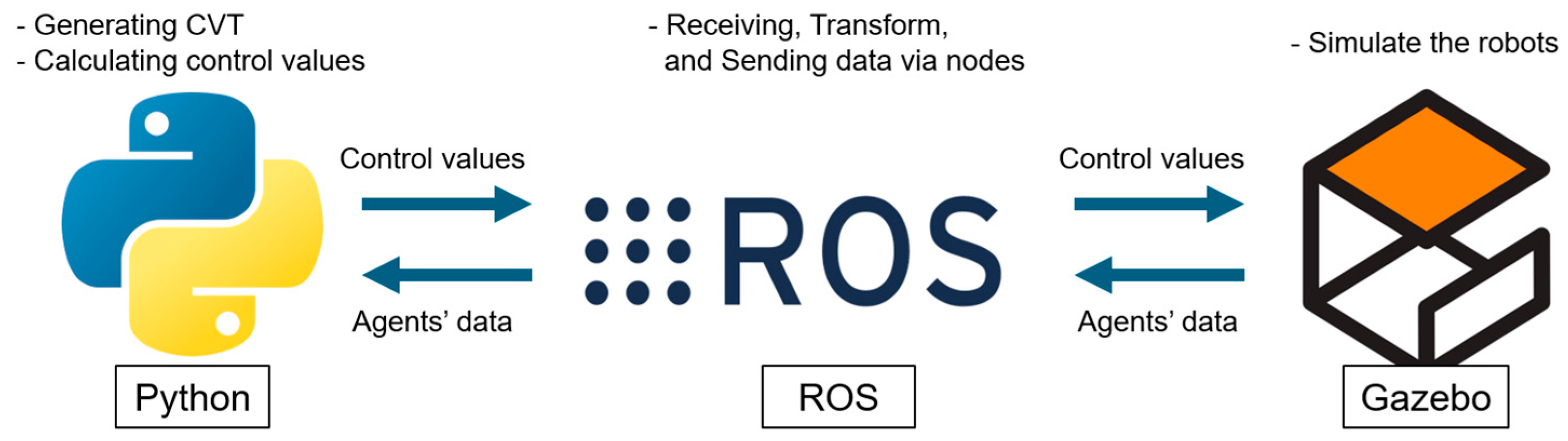
3.1. Simulation Environment

To validate the effectiveness of the proposed methodologies, a simulation environment was constructed for experimental testing. As shown in Figure 1, the Robot Operating System (ROS) Noetic Ninjemys, Python 3.8, and Gazebo 11 were integrated to simulate and develop the implementations of the 3D safe coverage controller within a three-dimensional space. These tools collectively lay the groundwork for testing and refining these advanced control strategies in a controlled yet realistic virtual environment.

Python is integral to scripting ROS nodes and executing the bulk of computational tasks within the simulation framework. The Python library Tess [34], specifically designed for this simulation, is tailored to calculate 3D CVT and analyze their characteristics thoroughly. In this study, Tess methodically partitions the three-dimensional space into cells, each distinctly defined by its centroid. It produces sophisticated tessellations that generate a series of cell objects, providing essential information such as volume, centroid, face count, and surface area—critical for the comprehensive analysis required in this research. Moreover, Python facilitates the implementation of safety barriers for agents and manages the calculation of their velocities, thereby ensuring dynamic and responsive interactions within the simulated environment.

ROS serves as a foundational framework for robot software development, offering a comprehensive suite of tools and libraries that support the construction and operation of robotic applications. In this simulation, ROS is employed as middleware to manage the connections between nodes, facilitating the reception and transmission of topics to and from various programs. Specifically, ROS is tasked with interpreting Python’s computational outputs and relaying these topics to the Gazebo Simulator. The version of ROS used in this study is ROS Noetic Ninjemys, which provides advanced capabilities and enhanced stability for complex simulations. In this study, the Hector Quadrotor model is employed to simulate multi-agent systems. This model represents a quadrotor helicopter, which is frequently utilized in the research and development of autonomous flight systems, as noted in [35,36]. It is fully integrated with the ROS, a versatile framework that facilitates the development of robotic software. Within ROS, the Hector Quadrotor package provides a comprehensive simulated environment where users can extensively test and refine algorithms for quadrotor control, navigation, and perception. Two principal features of the Hector Quadrotor package were instrumental in this study: firstly, environmental samples for Gazebo simulation, which allow the quadrotor to be evaluated under various scenarios, and secondly, simulated sensors and actuators, including an Inertial Measurement Unit (IMU), Global Positioning System (GPS), cameras, motors, and propellers. These tools collectively enable a realistic and dynamic testing environment for exploring the capabilities and behaviors of autonomous quadrotors.

Gazebo is a simulation software that enables users to design, test, and experiment with robots in intricately detailed environments without the necessity of physical prototypes, as documented in [37]. It integrates seamlessly with the ROS through plugins that facilitate communication between the simulation and ROS nodes. In this configuration, Gazebo receives input from ROS nodes via topics and utilizes these data to control agents within the simulation. Models of objects and agents are meticulously set up in the simulator and are manipulated based on the topics provided. The physical interactions between agents and objects are dynamically simulated using ODE (Open Dynamics Engine) version 0.16.2 physics engine [38] incorporated in Gazebo, enhancing the realism of the simulations. Additionally, the odometry data of the agents are relayed back to the ROS, where they are further processed and analyzed in Python. This loop of rapid data exchange and processing, repeating every few milliseconds, ensures the precise control of agents within the simulation, enabling a highly accurate replication of real-world dynamics.

3.2. Simulation Setup

The simulation environment is configured as a three-dimensional space measuring $40\times 40\times 40$ m, where the coordinates are bounded within −20 ≤ x ≤ 20, −20 ≤ y ≤ 20, and 0 ≤ z ≤ 40. According to the figures depicted, the starting area for the agents is marked in green. Each obstacle, represented as a crate measuring $10\times 10\times 10$ cubic meters, is strategically placed within the scene as illustrated in Figure 2. These obstacles are differentiated by varying colors to indicate their heights, providing a visual cue for the differing elevation levels throughout the simulation space. The layout for the simulation is categorized into two distinct types, symmetrical and asymmetrical, to demonstrate that the control system can effectively operate under varying conditions which may exhibit both uniformity and randomness. In the symmetrical layout, obstacles are arranged and stacked in different positions but form a symmetrical pattern when viewed from above, anticipating that each agent will follow a similar trajectory and pattern. Conversely, the asymmetrical layouts introduce more randomness in the placement of obstacles, aiming for unique and diverse agent trajectories and patterns, yet still adhering to the fundamental rules of goal-directed movement and collision avoidance. As shown in Figure 2, to represent both layout types, three distinct layouts have been designed—one for a symmetrical pattern and two for an asymmetrical pattern. In every scenario, agents are initialized at specified coordinates including [−6, 6, 0], [0, 6, 0], [6, 6, 0], [−6, −6, 0], [0, −6, 0], and [6, −6, 0], ensuring diverse starting conditions to rigorously test the system’s adaptability and performance in navigating complex three-dimensional environments.

To initiate the simulation, the 3D space is predefined, along with the starting points of eight quadrotors and the locations of 16 static obstacles, all specified in the launch files. The agents’ positions are relayed from the Gazebo simulator to the Python program via the ROS node, facilitating the computation of a 3D CVT within a $40\times 40\times 40 \mathrm{m}$³ container. This space is divided into eight Voronoi cells, each corresponding to one of the agents, utilizing the Tess library. As agents navigate the space, the Voronoi cells dynamically adapt based on the agents’ real-time positions. Each agent is programmed to move towards the centroid of its assigned cell at a maximum speed of 1 m per second. To compute velocities that ensure collision avoidance, the CBF is integrated into the system. A safety barrier of 8.7 m is established around each agent and obstacle, approximating the diameter of the smallest sphere capable of encompassing a $10\times 10\times 10 \mathrm{m}$³ cube. The mathematical model underpinning the 3D CBF informs the values applied within the program, where quadratic programming techniques are employed to resolve the equations and determine the optimal velocity for each agent to reach its target centroid without encountering collisions. The resulting velocity values are then communicated back to ROS, which dispatches Twist commands to adjust the quadrotors’ velocities in Gazebo accordingly. This loop continues until a predefined simulation endpoint is reached, ensuring the rigorous testing of the agents’ navigational abilities in complex three-dimensional environments.

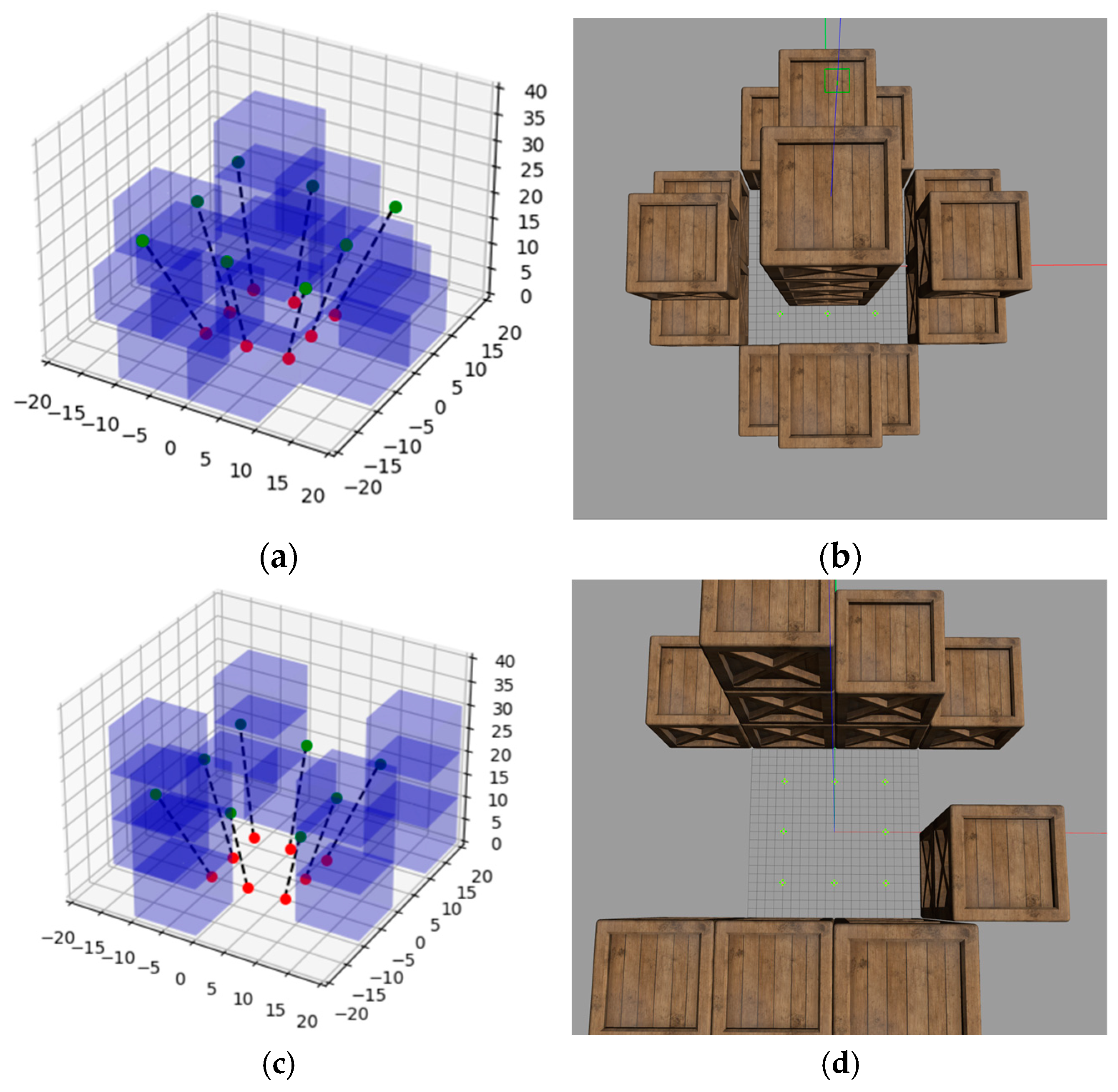
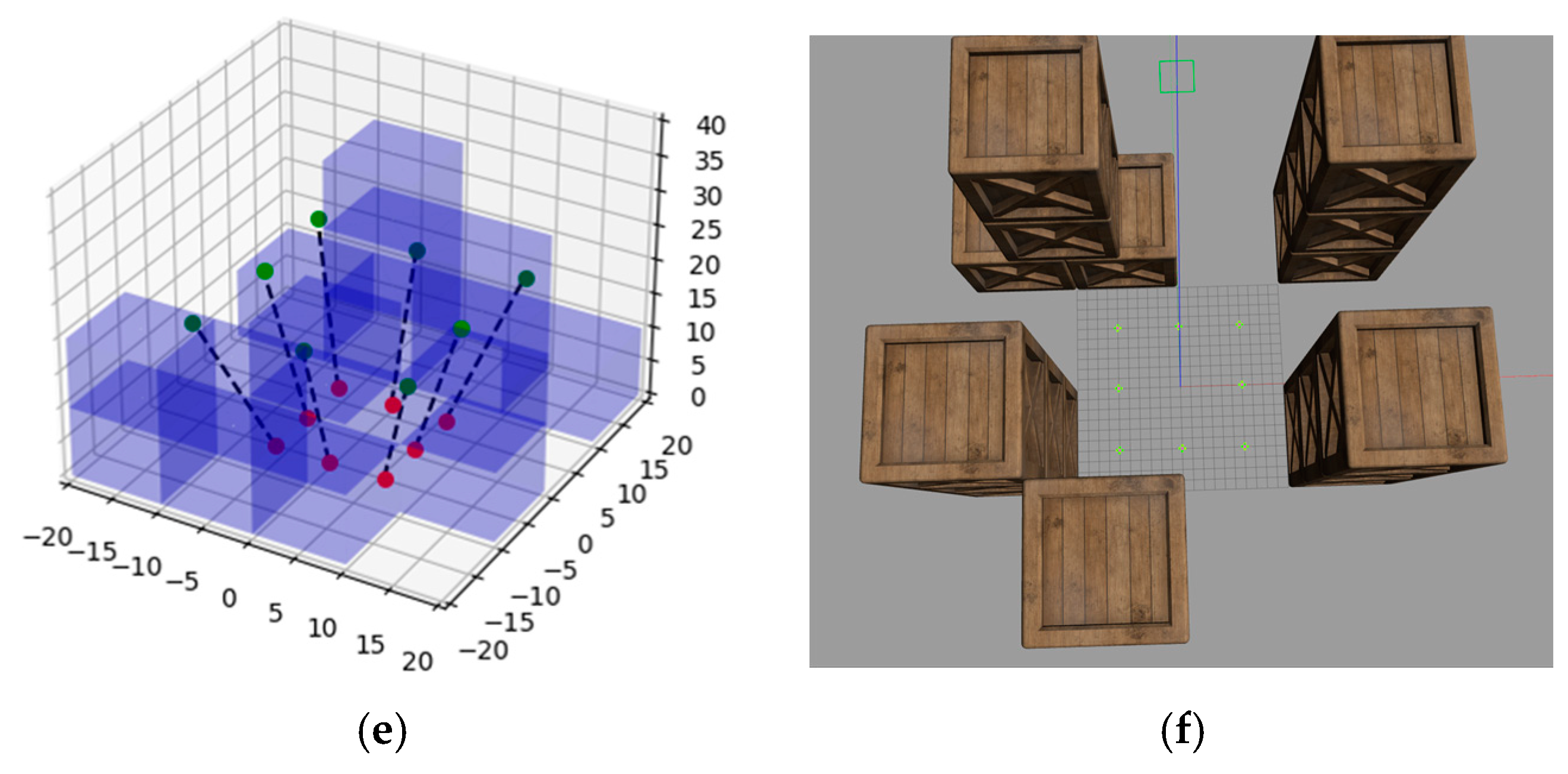
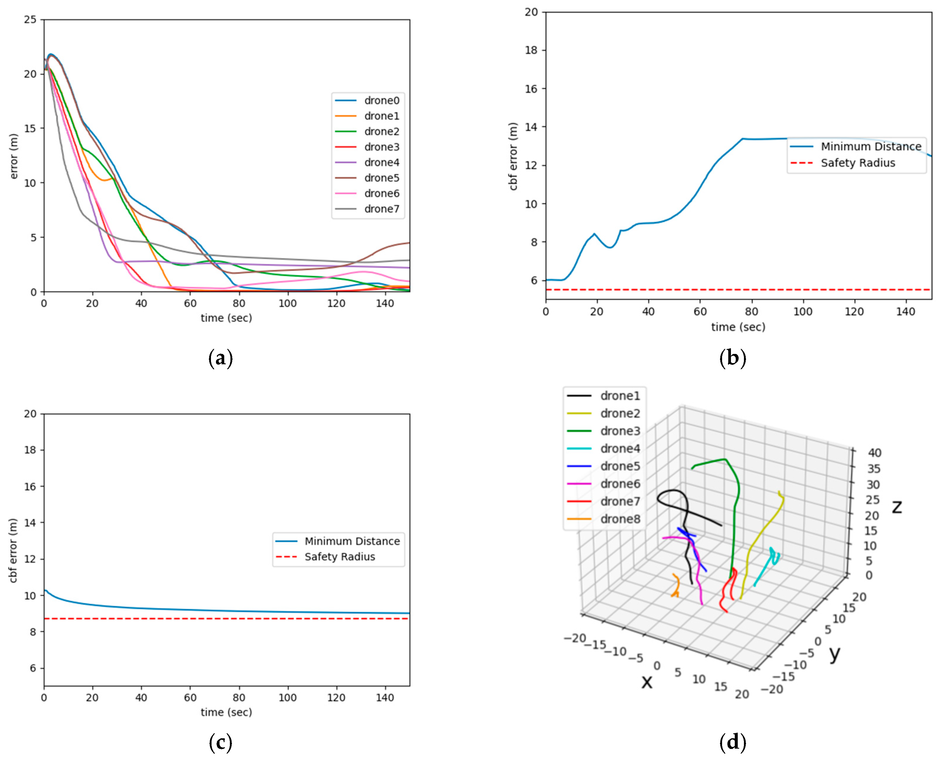
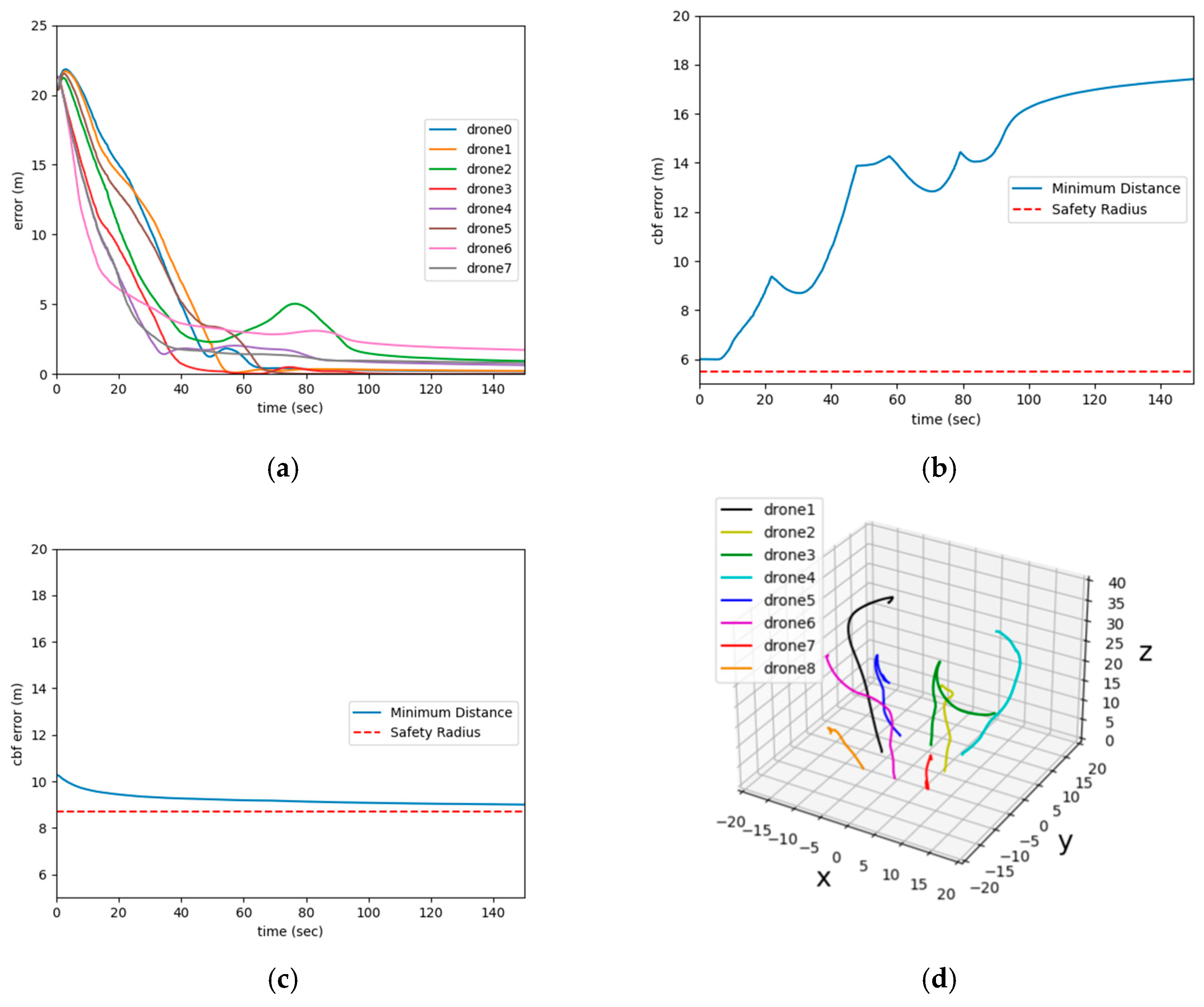
3.3. Simulation Results and Discussion

In this section, the feasibility of the 3D CVT with CBF control strategy is demonstrated through simulation. The simulation was executed over a period of 150 s, with initial conditions and subsequent outcomes at t = 0 s depicted in Figure 3. Each of the three distinct layouts was rigorously simulated and analyzed. The results from these simulations were methodically quantified and visualized in graphical format, detailing several critical aspects:

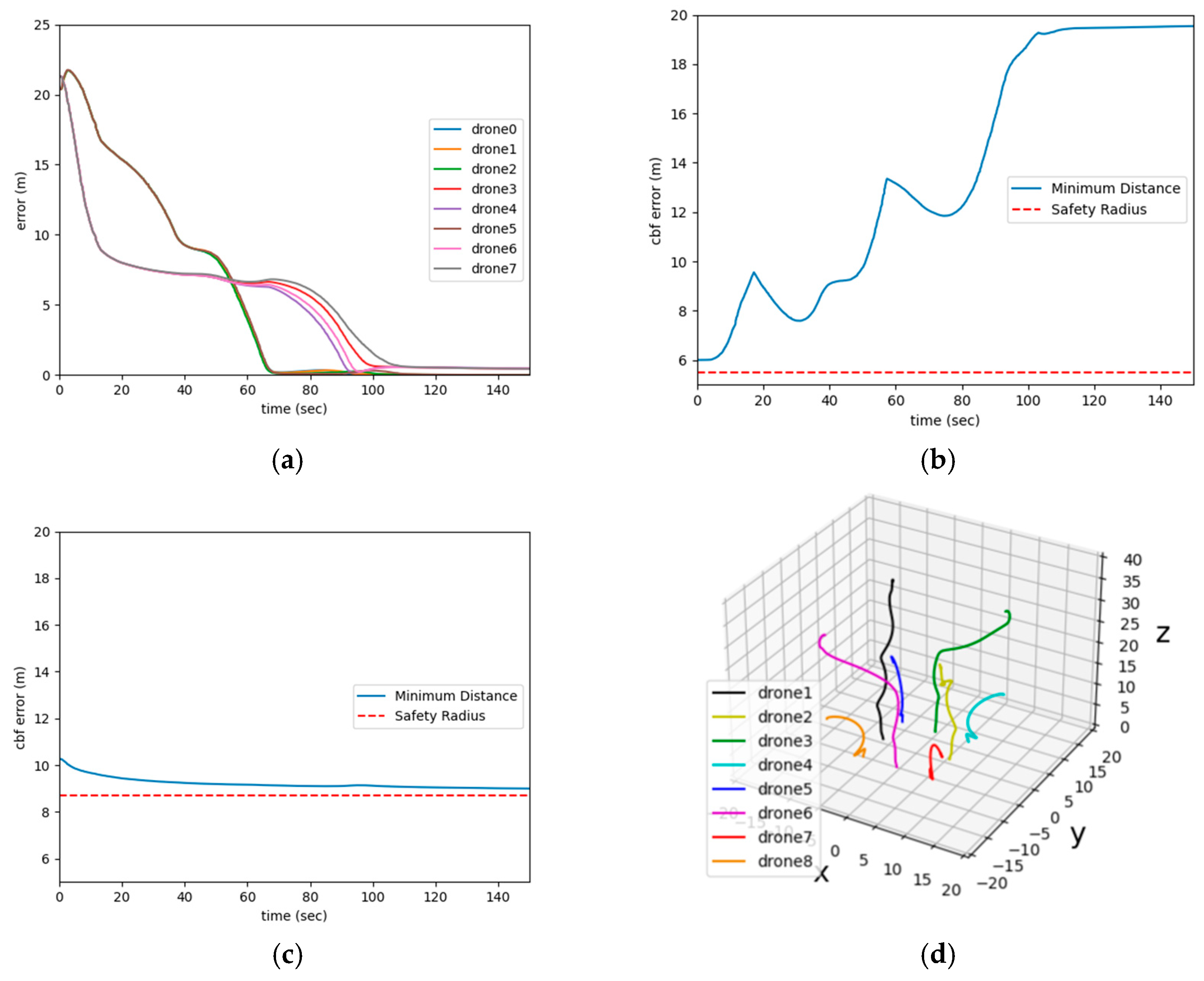
• The distance between agents and their respective goals;
• The shortest distance between agents over time;
• The shortest distance between agents and obstacles over time;
• The trajectories of the agents.

Figure 4 depicts the simulation results under a symmetrical environment layout, where multiple agents (labeled drone0 through drone7) navigate from their initial positions toward designated goal points while avoiding collisions. In Figure 4a, the curves show that the distance between each agent and its respective goal decreases over time, eventually stabilizing at values near zero. The nonzero asymptotes suggest that while agents approach their targets, they do not precisely land on the goal positions, likely due to proximity constraints imposed by surrounding agents or obstacles. Figure 4b tracks the shortest inter-agent distance, revealing that the agents do not converge toward one another despite their common goals; indeed, the minimum pairwise separation increases at later stages. This behavior indicates that the proposed controller maintains a distance above the safety radius (dashed line), thus preventing collisions even as agents move within proximity of their neighbors. Similarly, Figure 4c illustrates the shortest distance between agents and obstacles, confirming that the safety threshold is also upheld in agent–obstacle interactions. Although agents maneuver closer to obstacles over time, the minimum separation consistently remains above the prescribed safety margin. Finally, Figure 4d provides a three-dimensional view of each agent’s trajectory, illustrating the similarity in their paths that arises from the symmetrical obstacle arrangement. The agents exhibit parallel or mirrored movements in navigating around obstacles and heading to their destinations, reflecting both the symmetry of the layout and the uniform influence of the safe coverage controller. These results demonstrate that agents effectively reduce goal-reaching errors while maintaining the necessary distances to avoid collisions, showcasing both coverage performance and safety enforcement under symmetrical conditions.

Figure 5 and Figure 6 illustrate the outcomes in asymmetrical obstacle layouts, where agents navigate through more irregular environmental geometries compared to the symmetric case. In Figure 5a and Figure 6a, the distances between agents and their respective goals gradually decrease as the agents converge toward target locations, yet the time-varying nature of the 3D CVT intermittently causes these distances to rise when the Voronoi regions are reconfigured. This reflects the complex interplay among agent motions, dynamic centroid calculations, and uneven obstacle placement. From Figure 5b and Figure 6b, it is evident that agents consistently maintain safe inter-agent separations—none of the trajectories breach the prescribed minimum distance threshold. Meanwhile, Figure 5c and Figure 6c confirm that the shortest distances between agents and obstacles also remain above the safety radius, even as the agents maneuver closer to various barriers. These plots collectively demonstrate that collision-free operation is preserved at all times, thus highlighting the robustness of the 3D CBF in asymmetrical settings. Figure 5d and Figure 6d provide 3D perspectives of the agent trajectories, revealing more heterogeneous paths in comparison to the symmetric layout. The lack of regularity in obstacle positioning yields less uniform Voronoi cells, causing trajectories that appear more erratic or chaotic. Despite this irregularity, the system continues to uphold both coverage effectiveness—evidenced by a general downward trend in agent–goal distances—and collision avoidance, reflected in the safe separations plotted in Figure 5b,c and Figure 6b,c.

Table 1. Simulation results for all experiment layouts.

Experiment Layout	Average Final Error (m)	Convergence Time (s)
Symmetrical Layout	0.3	105
Asymmetrical Layout 1	1.8	80
Asymmetrical Layout 2	0.9	100

summarizes the simulation results for different experimental layouts. The Average Final Error represents the mean distance between agents and their respective goal positions at the end of the simulation. The Convergence Time indicates the duration required for the agents to reach their final stable positions.

Nonetheless, a trade-off emerges between safety and positional accuracy as, occasionally, an agent may be unable to settle exactly at its designated goal if it lies close to an obstacle’s safety boundary. For instance, in the simulation around t = 150 s, “drone6” fails to converge precisely to its target due to velocity restrictions imposed by the Control Barrier Function. These results underscore the effectiveness of the safe 3D coverage controller in ensuring collision-free navigation and adaptive coverage, even under the complexity and unpredictability introduced by asymmetrical obstacles.

The simulation results demonstrate the feasibility and effectiveness of the proposed safe 3D coverage control method, ensuring collision-free navigation and optimal coverage distribution. However, several aspects require further exploration to enhance the generalizability and practical applicability of the approach. One key aspect is the scalability of the system. While the current study considers a relatively small number of UAVs, expanding the system to include a significantly larger fleet, such as 80 or even 800 UAVs, will provide further insights into its computational feasibility and communication efficiency in large-scale multi-agent settings. Additionally, the assumption of a fully known environment with predetermined obstacle positions and target areas simplifies the problem but does not fully reflect real-world scenarios. Future efforts should focus on adapting the algorithm to unknown environments, where UAVs must rely on onboard sensors to acquire necessary information in real time, enabling autonomous navigation in dynamic and unpredictable conditions.

Beyond UAV applications, the proposed method has the potential to be extended to other autonomous robotic platforms, such as autonomous underwater vehicles for ocean exploration and coverage tasks in marine environments. Investigating the adaptability of the algorithm across different domains will provide broader insights into its versatility and robustness. Addressing these challenges will contribute to the development of more efficient and adaptable multi-agent coverage control strategies, enhancing their applicability to real-world scenarios.

4. Conclusions

In this study, a safe 3D coverage controller was formulated and rigorously validated, integrating coverage control with collision avoidance for multi-agent systems in three-dimensional spaces. The presented framework leverages 3D CVT to optimally distribute agents across a designated volume, coupled with a refined CBF mechanism that enforces collision-free trajectories in complex environments. Simulations in both symmetrical and asymmetrical layouts demonstrate that the proposed controller maintains robust coverage performance while consistently preserving safe distances between agents and obstacles. This confirms the feasibility and effectiveness of the safe 3D coverage controller and provides a foundation for future work on more sophisticated multi-agent deployments in dynamically evolving, high-dimensional domains.

Notwithstanding these positive results, certain limitations remain. The 3D CVT approach can be sensitive to parameter tuning when agents operate near constrained or irregular regions, and the current work relies primarily on simulation-based validation. Large-scale physical experiments might introduce additional uncertainties that are not explicitly accounted for in the present model. Moving forward, refining the density function or incorporating learning-based methods may enhance scalability and adaptability in evolving 3D environments. Adopting boundary-integral techniques for 3D CVT calculations could further reduce computational complexity, thereby supporting real-time implementations.

References

1. Bai, Y.; Tran Ngoc, P.T.; Nguyen, H.D.; Le, D.L.; Ha, Q.H.; Kai, K.; See To, Y.X.; Deng, Y.; Song, J.; Wakamiya, N.; et al. Swarm Navigation of Cyborg-Insects in Unknown Obstructed Soft Terrain. Nat. Commun. 2025, 16, 221. [Google Scholar] [CrossRef] [PubMed]
2. Wang, S.; Wan, J.; Zhang, D.; Li, D.; Zhang, C. Towards Smart Factory for Industry 4.0: A Self-Organized Multi-Agent System with Big Data-Based Feedback and Coordination. Comput. Netw. 2016, 101, 158–168. [Google Scholar] [CrossRef]
3. Xie, J.; Liu, C. Multi-Agent Systems and Their Applications. J. Int. Counc. Electr. Eng. 2017, 7, 189–197. [Google Scholar] [CrossRef]
4. Lee, J.H.; Kim, C.O. Multi-Agent Systems Applications in Manufacturing Systems and Supply Chain Management: A Review Paper. Int. J. Prod. Res. 2007, 46, 233–265. [Google Scholar] [CrossRef]
5. Dorri, A.; Kanhere, S.S.; Jurdak, R. Multi-Agent Systems: A Survey. IEEE Access 2018, 6, 28573–28593. [Google Scholar] [CrossRef]
6. Liang, J.; Li, Y.; Yin, G.; Xu, L.; Lu, Y.; Feng, J.; Shen, T.; Cai, G. A MAS-Based Hierarchical Architecture for the Cooperation Control of Connected and Automated Vehicles. IEEE Trans. Veh. Technol. 2022, 72, 1559–1573. [Google Scholar] [CrossRef]
7. Liang, J.; Lu, Y.; Yin, G.; Fang, Z.; Zhuang, W.; Ren, Y.; Xu, L.; Li, Y. A Distributed Integrated Control Architecture of AFS and DYC Based on MAS for Distributed Drive Electric Vehicles. IEEE Trans. Veh. Technol. 2021, 70, 5565–5577. [Google Scholar] [CrossRef]
8. Cortes, J.; Martinez, S.; Karatas, T.; Bullo, F. Coverage Control for Mobile Sensing Networks. IEEE Trans. Robot. Autom. 2004, 20, 243–255. [Google Scholar] [CrossRef]
9. Lee, S.G.; Diaz-Mercado, Y.; Egerstedt, M. Multi-Robot Control Using Time-Varying Density Functions. IEEE Trans. Robot. 2015, 31, 489–493. [Google Scholar] [CrossRef]
10. Miah, S.; Fallah, M.M.H.; Spinello, D. Non-Autonomous Coverage Control with Diffusive Evolving Density. IEEE Trans. Autom. Control 2017, 62, 5262–5268. [Google Scholar] [CrossRef]
11. Miah, S.; Panah, A.Y.; Fallah, M.M.H.; Spinello, D. Generalized Non-Autonomous Metric Optimization for Area Coverage Problems with Mobile Autonomous Agents. Automatica 2017, 80, 295–299. [Google Scholar] [CrossRef]
12. Chevet, T.; Maniu, C.S.; Vlad, C.; Zhang, Y. Guaranteed Voronoi-Based Deployment for Multi-Agent Systems under Uncertain Measurements. In Proceedings of the 18th European Control Conference (ECC), Naples, Italy, 25–28 June 2019. [Google Scholar]
13. Li, S.; Li, B.; Yu, J.; Zhang, L.; Zhang, A.; Cai, K. Probabilistic Threshold k-Ann Query Method Based on Uncertain Voronoi Diagram in Internet of Vehicles. IEEE Trans. Intell. Transp. Syst. 2021, 22, 3592–3602. [Google Scholar] [CrossRef]
14. Zhou, D.; Wang, Z.; Bandyopadhyay, S.; Schwager, M. Fast, Online Collision Avoidance for Dynamic Vehicles Using Buffered Voronoi Cells. IEEE Robot. Autom. Lett. 2017, 2, 1047–1054. [Google Scholar] [CrossRef]
15. Wang, M.; Wang, Z.; Paudel, S.; Schwager, M. Safe Distributed Lane Change Maneuvers for Multiple Autonomous Vehicles Using Buffered Input Cells. In Proceedings of the 2018 IEEE International Conference on Robotics and Automation (ICRA), Brisbane, Australia, 21–25 May 2018; pp. 4678–4684. [Google Scholar]
16. Pierson, A.; Rus, D. Distributed Target Tracking in Cluttered Environments with Guaranteed Collision Avoidance. In Proceedings of the 2017 International Symposium on Multi-Robot and Multi-Agent Systems (MRS), Cambridge, MA, USA, 4–5 December 2017; pp. 83–89. [Google Scholar]
17. Pierson, A.; Schwarting, W.; Karaman, S.; Rus, D. Weighted Buffered Voronoi Cells for Distributed Semi-Cooperative Behavior. In Proceedings of the 2020 IEEE International Conference on Robotics and Automation (ICRA), Paris, France, 31 May–31 August 2020; pp. 5611–5617. [Google Scholar]
18. Garg, K.; Panagou, D. Robust Control Barrier and Control Lyapunov Functions with Fixed-Time Convergence Guarantees. In Proceedings of the 2021 American Control Conference (ACC), New Orleans, LA, USA, 25–28 May 2021; pp. 2292–2297. [Google Scholar]
19. Nguyen, Q.; Sreenath, K. Robust Safety-Critical Control for Dynamic Robotics. IEEE Trans. Autom. Control 2022, 67, 1073–1088. [Google Scholar] [CrossRef]
20. Verginis, C.K.; Djeumou, F.; Topcu, U. Safety-Constrained Learning and Control Using Scarce Data and Reciprocal Barriers. arXiv 2021, arXiv:2105.06526. [Google Scholar]
21. Fungtammasan, K.; Bai, Y.; Svinin, M.; Matsuno, F.; Magid, E.; Suthakorn, J. Adaptive Coverage Control for Dynamic Pattern Generation. In Proceedings of the 2022 13th Asian Control Conference (ASCC), Pusan, Republic of Korea, 4–7 May 2022; pp. 1404–1408. [Google Scholar]
22. Bai, Y.; Wang, Y.; Xiong, X.; Song, J.; Svinin, M. Safe Adaptive Multi-Agent Coverage Control. IEEE Control Syst. Lett. 2023, 7, 3217–3222. [Google Scholar] [CrossRef]
23. Bai, Y.; Wang, Y.; Svinin, M.; Magid, E.; Sun, R. Function Approximation Technique Based Immersion and Invariance Control for Unknown Nonlinear Systems. IEEE Control Syst. Lett. 2020, 4, 934–939. [Google Scholar] [CrossRef]
24. Bai, Y.; Svinin, M.; Yamamoto, M. Function Approximation Based-Control for Non-Square Systems. SICE J. Control Meas. Syst. Integr. 2018, 11, 477–485. [Google Scholar] [CrossRef]
25. Chertovskih, R.; Ribeiro, V.M.; Gonçalves, R.; Aguiar, A.P. Sixty Years of the Maximum Principle in Optimal Control: Historical Roots and Content Classification. Symmetry 2024, 16, 1398. [Google Scholar] [CrossRef]
26. Meng, X.; Houshmand, A.; Cassandras, C.G. Multi-Agent Coverage Control with Energy Depletion and Repletion. In Proceedings of the 2018 IEEE Conference on Decision and Control (CDC), Miami, FL, USA, 17–19 December 2018; IEEE: New York, NY, USA, 2018. [Google Scholar]
27. Bonnet, B. A Pontryagin Maximum Principle in Wasserstein Spaces for Constrained Optimal Control Problems. ESAIM Control Optim. Calc. Var. 2019, 25, 52. [Google Scholar] [CrossRef]
28. Segawa, K.; Hayashi, N.; Takai, S. 2D Voronoi Coverage Control with Gaussian Density Functions by Line Integration. SICE J. Control Meas. Syst. Integr. 2017, 10, 110–116. [Google Scholar]
29. Xu, B.; Sreenath, K. Safe Teleoperation of Dynamic UAVs through Control Barrier Functions. In Proceedings of the 2018 IEEE International Conference on Robotics and Automation (ICRA), Brisbane, Australia, 21–25 May 2018; pp. 7848–7855. [Google Scholar]
30. Wang, L.; Ames, A.D.; Egerstedt, M. Safe Certificate-Based Maneuvers for Teams of Quadrotors Using Differential Flatness. In Proceedings of the 2017 IEEE International Conference on Robotics and Automation (ICRA), Singapore, 29 May–3 June 2017; pp. 3293–3298. [Google Scholar]
31. Siri, F.C.; Song, J.; Svinin, M. Safe Coverage Control of Multi-Agent Systems and Its Verification in ROS/Gazebo Environment. Information 2024, 15, 462. [Google Scholar] [CrossRef]
32. Siri, F.C.; Song, J.; Svinin, M. Experimental Verification of Coverage Control of Multi-Agent Systems with Obstacle Avoidance. J. Eng. 2024, 12, e70045. [Google Scholar] [CrossRef]
33. Xu, X.; Tabuada, P.; Grizzle, J.W.; Ames, A.D. Robustness of Control Barrier Functions for Safety-Critical Control. IFAC—PapersOnLine 2015, 48, 54–61. [Google Scholar] [CrossRef]
34. Tess. Available online: https://tess.readthedocs.io/en/latest/ (accessed on 10 May 2024).
35. Open Source Robotics Foundation. Available online: https://wiki.ros.org/hector_quadrotor (accessed on 10 May 2024).
36. Rafalamao/Hector-Quadrotor-Noetic: Hector Quadrotor Ported to ROS Noetic with Gazebo 11. Available online: https://github.com/RAFALAMAO/hector-quadrotor-noetic (accessed on 12 May 2024).
37. Open Source Robotics Foundation. Available online: https://gazebosim.org/about (accessed on 15 May 2024).
38. Open Dynamic Engine. Available online: https://ode.org (accessed on 15 May 2024).
Figure 1. Simulation environment.
Actuators 14 00186 g001
Figure 2. Simulation scenario layout setup. (a) Symmetrical layout, (b) asymmetrical layout 1, (c) asymmetrical layout 2, (d) color label3.2. simulation setup.
Actuators 14 00186 g002
Figure 3. The initial and target positions of the drones in simulation scenarios. (a) Symmetrical layout, (b) symmetrical layout, (c) asymmetrical layout 1, (d) asymmetrical layout 1, (e) asymmetrical layout 2, (f) asymmetrical layout 2 .Subfigure (a,c,e) presents a three-dimensional perspective of the environment. The red markers represent the initial positions of the agents, while the green markers indicate their corresponding goal locations. Subfigure (b,d,f) provides a top-down view of the environment.
Actuators 14 00186 g003aActuators 14 00186 g003b
Figure 4. Simulation results for symmetrical layout. (a) Distance between agents and goals, (b) shortest distance between agents, (c) shortest distance between agents and obstacles, (d) agents’ trajectories.
Actuators 14 00186 g004
Figure 5. Simulation results for asymmetrical layout 1. (a) Distance between agents and goals, (b) shortest distance between agents, (c) shortest distance between agents and obstacles, (d) agents’ trajectories.
Actuators 14 00186 g005
Figure 6. Simulation results for asymmetrical layout 2. (a) Distance between agents and goals, (b) shortest distance between agents, (c) shortest distance between agents and obstacles, (d) agents’ trajectories.
Actuators 14 00186 g006