Event-Triggered Bipartite Formation Control for Switched Nonlinear Multi-Agent Systems with Function Constraints on States

Abstract

A distributed adaptive fuzzy event-triggered bipartite formation tracking control scheme is proposed for switched nonlinear multi-agent systems (MASs) with function constraints on states. Fuzzy logic systems (FLSs) are used to identify uncertain items. To improve the transient performance of the system, a fixed-time prescribed performance function (FTPPF) is introduced to make the formation error converge to a prescribed boundary range within a fixed time. Considering that the state constraint boundary is restricted by multiple pieces of information (historical state, topological relationship, neighbor agent output, leader signal and time), a tan-type barrier Lyapunov function (BLF) is constructed to address the challenges brought by the state function constraint. The shortcoming of the “explosion of complexity” is compensated by fusing the backstepping control and command filter. To mitigate the communication burden while ensuring a steady-state performance, a distributed event-triggered fixed-time bipartite formation control scheme is proposed. Finally, the performance of the proposed control method is verified by an MAS consisting of four followers and one leader.

1. Introduction

With the developments of information network technology in control theory, the multi-agent systems (MASs), which integrate the capabilities of sensing, computing, execution, and decision making, have received widespread attention and have achieved some outstanding results in linear multi-agent systems [1,2,3]. Compared with linear systems, nonlinear models can more accurately describe the dynamic behavior of agents in actual systems. In recent years, distributed collaborative control methods based on adaptive fuzzy [4,5] or neural networks [6,7] and combined with the backstepping control method have further promoted the development of MAS control theory [8,9,10,11]. However, the above studies are based on cooperative relationships. In actual tasks, cooperative relationships are often accompanied by competitive relationships. Therefore, a more practical approach is to use a symbolic graph to describe the connection relationship between agents. On this basis, bipartite consensus control has been developed to satisfy actual mission requirements [12,13,14,15,16]. On the one hand, the consumption of limited resources caused by frequent communication between agents is a problem that cannot be ignored. For highly flexible and maneuverable agents such as drones and unmanned ships, the resources carried by its carriers are limited, and continuous communication or controller updates will put great pressure on the systems. As a non-periodic sampling strategy, event-triggered control (ETC) solves the problem of system communication pressure while ensuring system performance according to the designed trigger conditions [17,18,19,20]. Therefore, it has far-reaching significance and high application value for studying collaborative control under the event-triggered mechanism [21,22,23,24,25].

As an important research direction of collaborative control for MASs, formation control has broad application prospects in the military, civil, and industrial fields. Some formation control schemes were proposed in [26,27] based on cooperative relationships. Due to the existence of competitive relationships, the tasks of formation realization and maintenance are more challenging. Bipartite formation control refers to the existence of competition and cooperation relationships between agents, and two opposite formation states are achieved under this relationship [28]. To better meet the actual task requirements, some bipartite formation control methods are proposed in [29,30,31,32,33,34,35]. The bipartite formation control problem was studied in [29,30] for linear multi-agent systems. In [31], a multi-robot formation control was completed under communication time-delays. Bipartite formation control algorithms with multiple leaders were proposed in [32,33,34]. Under aperiodic denial of service attacks, reference [35] studied the bipartite formation control of MAS with fixed and switching topologies. In order to save resources, an optimized formation control scheme was proposed in [36], and the obstacle avoidance/collision task was completed in a bipartite formation. However, it is also necessary to consider realistic constraints when implementing formation control to maintain and ensure the stability, safety, and high-performance operation of actual systems, which are ignored by the above research methods.

Due to physical conditions and safety restrictions, the actual physical systems need to meet certain conditions during operation, such as the velocity of wheeled mobile robot [37] and the temperature, pressure, and material concentration of chemical reaction systems [38]. Otherwise, the system control performance may deteriorate. The barrier Lyapunov function (BLF) and nonlinear mapping method have become the main methods to solve constraints and have achieved remarkable results in nonlinear MASs [39,40,41,42]. Currently, some constraints on bipartite consensus methods have also been reported [43,44,45,46,47]. A constant constraint boundary on state was solved in [43] based on BLF. Asymmetric constant constraint boundary on output in [44] and time-varying con-strained boundary on states in [45,46] were solved based on the nonlinear mapping function method. Considering the more complex working environment and strict constraint requirements, a type of constraint boundary related to historical states and time was solved in [47]. On the other hand, to achieve precise adjustment and optimal control, [48,49] considered the constraints of the tracking error and proposed the fixed-time prescribed performance function (FTPPF) control method to make sure the tracking error would fall into the prescribed boundary within a predesigned amount of time. However, the above control schemes are only restricted to non-switched MASs.

Since the properties of the switched systems are not just the superposition of subsystem properties, its special properties make the above control schemes unsuitable for switched MASs. At present, distributed-based control for switched MASs has gradually developed [50,51,52,53,54,55], which provides theoretical support for the further improvement of switched MASs. Under the switching topology, the consensus problem for switched MASs with unknown deception attacks in [50] is solved. By introducing dynamic signals, the unmodeled dynamics are addressed in [51]. References [52,53] implemented consensus control based on state-dependent and mode-dependent average dwell time switching protocols, respectively. A prescribed performance control scheme was proposed in [54] for the formation tracking problem with dynamic obstacle avoidance and range constraints. However, bipartite formation control for switched nonlinear MASs with function constraints on states has not been investigated yet.

Inspired by the above studies and taking into account the communication burden, explosion of complexity, and transient performance issues, an adaptive bipartite time-varying formation control scheme for switched MASs with function constraints on states is proposed. The main innovations are summarized as follows:

(1)

An adaptive fuzzy event-triggered bipartite time-varying formation control scheme is proposed, which expands the scope of practical application and alleviates the communication burden and explosion of complexity.

(2)

Compared with the bipartite formation control scheme proposed in [26,27,28,29,30], the proposed control scheme is based on the FTPPT. Specifically, the formation error falls into the prescribed performance boundary within a predefined time.

(3)

Considering the constraint boundaries related to historical states and time, it is more adaptable to complex external environments compared with static constraints [43,44] or constraint boundaries that only depend on time [45,46].

2. System Description and Preliminaries

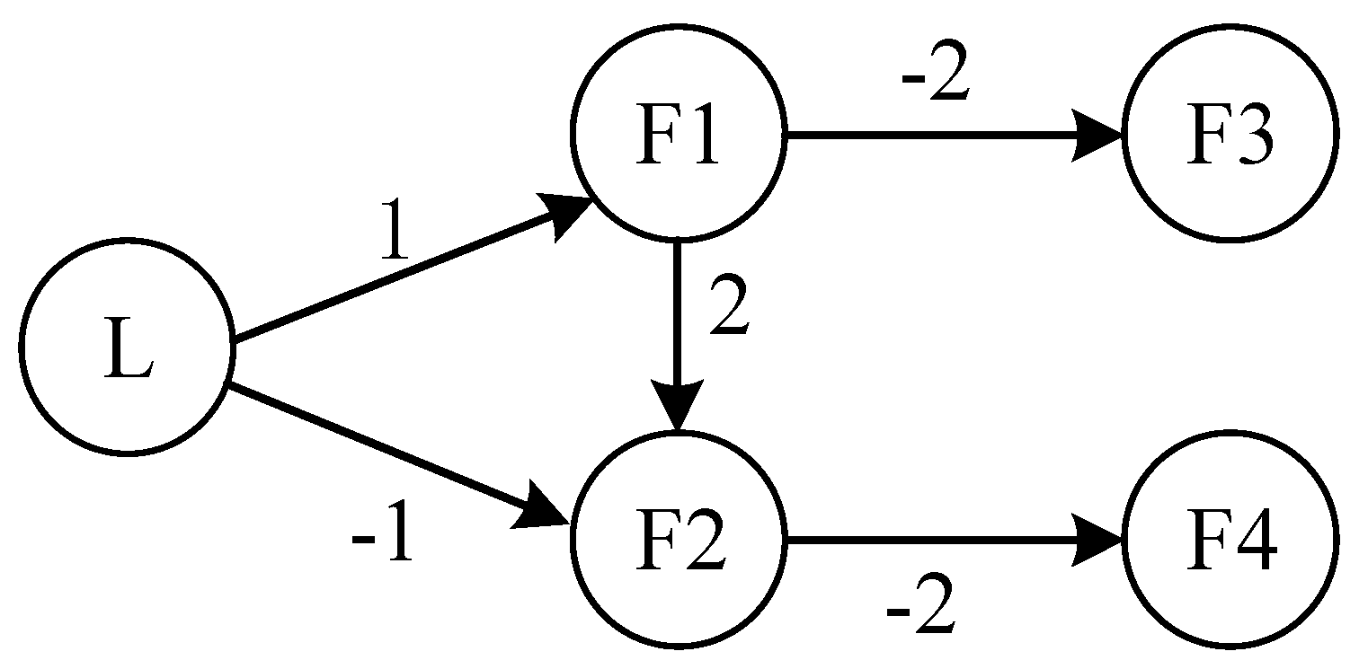
2.1. Graph Theory

A directed graph $\mathfrak{A}=\left(\Gamma ,\aleph ,A\right)$ is presented to describe the topological behavior and information exchange between agents. $\Gamma =\left\{c_1,c_2,\cdots ,c_S\right\}$ is the node set; $\aleph \subseteq \Gamma \times \Gamma$ is the set of edges connecting two vertices. $A=[a_{\mathcal{l},l}]\in R^{S\times S}$ stands for the adjacency matrix. $a_{\mathcal{l},l}\ne 0$ means the agent $c_{\mathcal{l}}$ can accept the information sent by agent $c_l$; otherwise, $a_{\mathcal{l},l}=0$. The weight $a_{\mathcal{l},l}>0$ indicates cooperation and $a_{\mathcal{l},l}<0$ indicates competition. The Laplacian matrix is $L=D-A$, where $D=diag\left\{d_1,\cdots ,d_S\right\}$ with $d_{\mathcal{l}}={\displaystyle \sum _{l=1}^S\left|a_{\mathcal{l},l}\right|}$. A path on $\mathfrak{A}$ from $c_{\mathcal{l}0}$ to $c_{\mathcal{l}k}$ is a sequence of distinct vertices ($c_{\mathcal{l}0},\cdots ,c_{\mathcal{l}k}$), where $\left(c_{\mathcal{l}j-1},c_{\mathcal{l}j}\right)\in \aleph$ for $j=1,\cdots ,k$. Define $B=diag\left\{\left|b_1\right|,\cdots ,\left|b_S\right|\right\}$, where $b_{\mathcal{l}}$ expresses the edge weight between the leader and the $\mathcal{l}$-th follower; $b_{\mathcal{l}}>0$ and $b_{\mathcal{l}}<0$ indicate cooperative and competitive relationships, respectively. $b_{\mathcal{l}}=0$ means no information exchange.

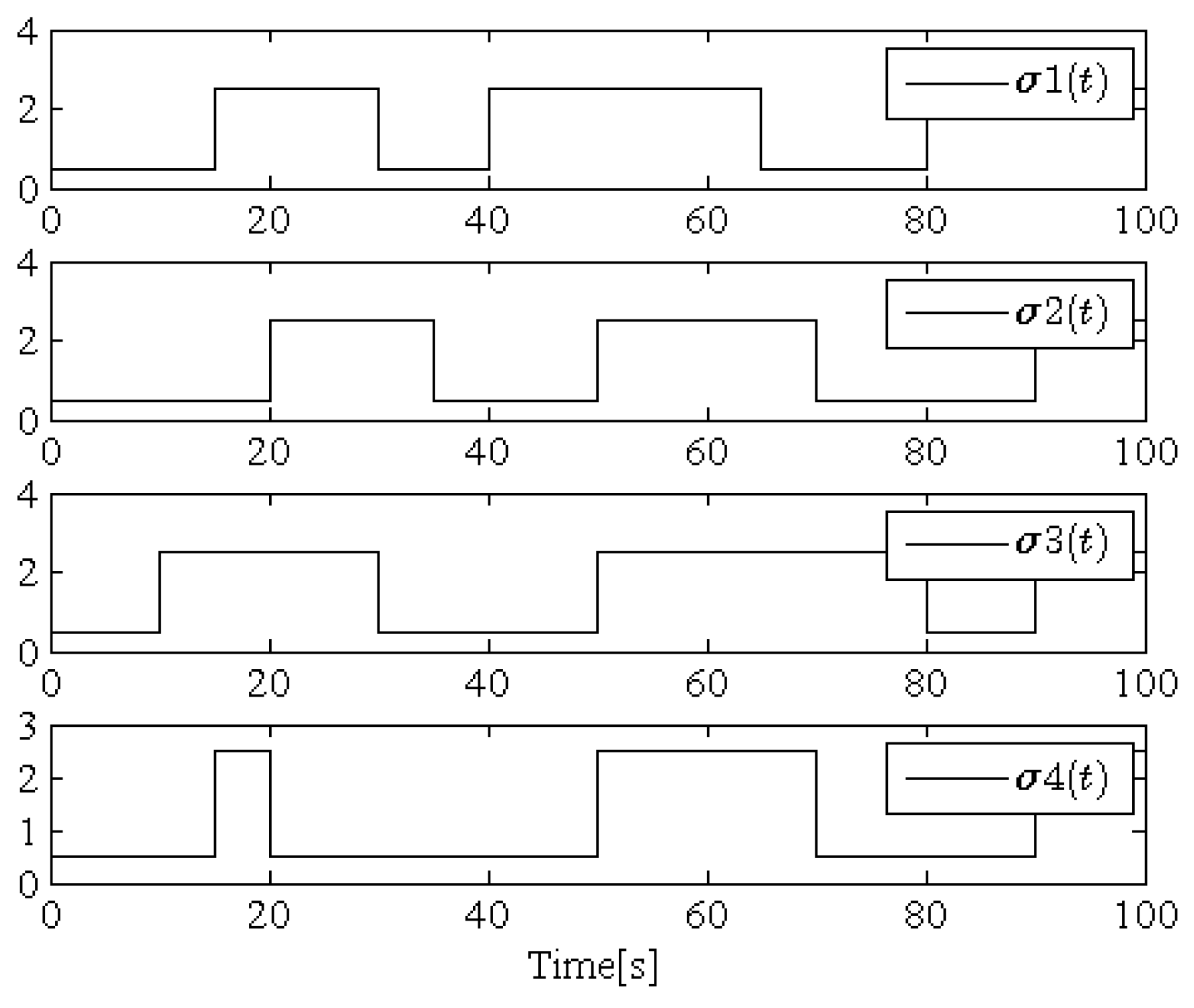
2.2. Switched MASs Description

This study focuses on the switched nonlinear MAS, which consists of $S$ followers and one leader. The dynamics of the $\mathcal{l}$-th follower are given as:

$$\begin{gathered} {\dot{x}}_{\mathcal{l},q}=x_{\mathcal{l},q+1}+f_{\mathcal{l},q}^{{\sigma }_{\mathcal{l}}\left(t\right)}\left({\overline{x}}_{\mathcal{l},q}\right) \\ {\dot{x}}_{\mathcal{l},S_{\mathcal{l}}}=u_{\mathcal{l}}+f_{\mathcal{l},S_{\mathcal{l}}}^{{\sigma }_{\mathcal{l}}\left(t\right)}\left({\overline{x}}_{\mathcal{l},S_{\mathcal{l}}}\right) \end{gathered}$$

$$y_{\mathcal{l}}=x_{\mathcal{l},1}, 1\le \mathcal{l}\le S, 1\le q\le S_{\mathcal{l}}-1$$

(1)

where $x_{\mathcal{l},q}={\left[x_{\mathcal{l},1},\cdots ,x_{\mathcal{l},q}\right]}^T\in R^q$ ($q=1,\cdots ,S_{\mathcal{l}}$) and $x_{\mathcal{l}}={\overline{x}}_{\mathcal{l},S_{\mathcal{l}}}$ are the state vector. $u_{\mathcal{l}}\in R^S$ and $y_{\mathcal{l}}\in R^S$ are the input and output of agent $\mathcal{l}$. ${\sigma }_{\mathcal{l}}\left(t\right)\in \left[0,\infty \right)\to {\Upsilon }_{\mathcal{l}}=\left\{1,2,\cdots ,{\overline{\Upsilon }}_{\mathcal{l}}\right\}$ means the switching law, with ${\overline{\Upsilon }}_{\mathcal{l}}$ being the number of subsystems. If ${\sigma }_{\mathcal{l}}\left(t\right)=k\left(k\in {\Upsilon }_{\mathcal{l}}\right)$, the $k$-th subsystem is active. $f_{\mathcal{l},q}^k\left({\overline{x}}_{\mathcal{l},q}\right)$ represents unknown smooth nonlinear functions.

All states of the $\mathcal{l}$-th follower are subjected to functional constraints, i.e.,

$$\left|x_{\mathcal{l},q}\right|\le k_{\mathcal{l},q}\left({\overline{\chi }}_{\mathcal{l},q-1},t\right),q=1,\cdots ,S_{\mathcal{l}}$$

with $k_{\mathcal{l},q}\left({\overline{\chi }}_{\mathcal{l},q-1},t\right)$ being a known smooth function related to multi-information, ${\overline{\chi }}_{\mathcal{l},q-1}=\left[{\overline{\chi }}_{\mathcal{l},0}^T,\right.{\left.x_{\mathcal{l},1},\cdots ,x_{\mathcal{l},q-1}\right]}^T$, ${\overline{\chi }}_{\mathcal{l},0}=\left[a_{\mathcal{l},1}{y}_1,\right.\cdots ,$ ${\left.a_{\mathcal{l},S}{y}_S,b_{\mathcal{l}}{y}_r\right]}^T$, and $y_r$ is the leader signal.

Control objectives: (1) By achieving fast bipartite formation tracking control, the formation errors can converge to a minimum set close to the origin of the prescribed performance. (2) All states of the system satisfy prescribed constraint boundaries. (3) All signals are bounded, and the Zeno behavior can be avoided.

Assumption 1.

For each follower in a formation, it is assumed that there is a directed path between at least one leader and that follower.

Assumption 2.

For the leader signal, $y_r$ and ${\dot{y}}_r$ are satisfied: $\left|y_r\right|\le Y_0\left(t\right)\le k_{\mathcal{l},1}\left({\overline{\chi }}_{\mathcal{l},0},t\right)$; $\left|{\dot{y}}_r\right|\le Y_1$, where $Y_1>0$.

Lemma 1

([18]). For $\forall ƛ>0,\rho \in R$, the inequality holds:

$$0\le \left|\rho \right|-\rho \tan \left({\displaystyle \frac{\rho }{ƛ}}\right)\le 0.2785ƛ$$

(2)

Lemma 2

([1,2]). Consider a continuous function $f\left(x\right)$ defined on a compact set $\Omega$. For $\forall \epsilon >0$, there exists a FLS$\left(y={\theta }^T\phi \left(x\right)\right)$ satisfying:

$$\underset{x\in \Omega }{\sup }\left|f\left(x\right)-{\theta }^{\mathrm{T}}\phi \left(x\right)\right|\le \epsilon$$

(3)

where $y={\displaystyle \sum _{\kappa =1}^{\iota }{\overline{y}}_{\kappa }}{\Pi }_{i=1}^n{\mu }_{F_i^{\iota }}\left(x_i\right)/{\displaystyle \sum _{\kappa =1}^{\iota }{\Pi }_{i=1}^n{\mu }_{F_i^{\iota }}\left(x_i\right)}$, $\iota$ is the number of fuzzy rules, and ${\overline{y}}_{\kappa }={\max }_{y\in R}{\mu }_{G^{\kappa }}\left(y\right)$, ${\theta }^T=\left[{\overline{y}}_1,\cdots ,\overline{y}\right]=\left[{\theta }_1,\cdots ,{\theta }_{\iota }\right]$. $\phi \left(x\right)={\left[{\phi }_1\left(x\right),\cdots ,{\phi }_{\iota }\left(x\right)\right]}^T$ is defined as the fuzzy-basis function, ${\phi }_{\kappa }\left(x\right)={\Pi }_{i=1}^n{\mu }_{F_i^{\iota }}\left(x_i\right)/{\displaystyle \sum _{\kappa =1}^{\iota }{\Pi }_{i=1}^n{\mu }_{F_i^{\iota }}\left(x_i\right)}$, ${\mu }_{G^{\kappa }}\left(y\right)$, and ${\mu }_{F_i^{\iota }}\left(x_i\right)$ is the membership function.

3. Event-Triggered Bipartite Formation Controller Design Based on FTPPF and Stability Analysis

The formation error is defined as:

$$z_{\mathcal{l},1}={\displaystyle \sum _{l=1}^S\left|a_{\mathcal{l},l}\right|}\left(y_{\mathcal{l}}-{\delta }_{\mathcal{l}}\left(t\right)-sign(a_{\mathcal{l},l})y_{l,1}-{\delta }_l\left(t\right)\right)+\left|b_{\mathcal{l}}\right|\left(y_{\mathcal{l},1}-{\delta }_{\mathcal{l}}\left(t\right)-sign(b_{\mathcal{l}})y_r\right)$$

(4)

where ${\delta }_{\mathcal{l}}\left(t\right)$ and ${\delta }_l\left(t\right)$ is denoted as the time-varying expected formation.

Lemma 3

([44]). The consensus tracking error $e_{\mathcal{l},1}=y_{\mathcal{l}} -$ $sign(b_{\mathcal{l}})y_r$, $e={\left[e_{1,1},\cdots ,e_{S,1}\right]}^T$ denotes $z_1={\left[z_{1,1},\cdots ,z_{S,1}\right]}^T$. Then, it holds that:

$$‖e‖\le {\displaystyle \frac{‖z_1‖}{{\lambda }_{\min }\left(L+B\right)}}$$

(5)

To ensure that the formation error of each agent strictly enters and remains within the prescribed boundaries with the pre-designed time, the following conditions should be met:

$$-{\omega }_{\mathcal{l}}\left(t\right)<z_{\mathcal{l},1}<{\omega }_{\mathcal{l}}\left(t\right),\forall t\ge 0$$

(6)

where  ${\omega }_{\mathcal{l}}\left(t\right)$ is the FTPPF.

Definition 1

([49]). The FTPPF ${\omega }_{\mathcal{l}}\left(t\right)$ should satisfy the following properties: (1) ${\omega }_{\mathcal{l}}\left(t\right)>0$ and ${\dot{\omega }}_{\mathcal{l}}\left(t\right)\le 0$; (2) $\underset{t\to T_{\mathcal{l}}}{\lim }{\omega }_{\mathcal{l}}\left(t\right)={\omega }_{T_{\mathcal{l}}}$.

According to Definition 1, ${\omega }_{\mathcal{l}}\left(t\right)$ can be defined as:

$${\omega }_{\mathcal{l}}\left(t\right)=\left\{\begin{array}{ll}{\left({\omega }_{\mathcal{l},0}^{h_{\mathcal{l}}}-h_{\mathcal{l}}{\xi }_{\mathcal{l}}t\right)}^{1/h_{\mathcal{l}}}+{\omega }_{T_{\mathcal{l}}},& t<T_{\mathcal{l}}\\ {\omega }_{T_{\mathcal{l}}},& t\ge T_{\mathcal{l}}\end{array}\right.$$

(7)

where ${\omega }_{T_{\mathcal{l}}}>0$ represents the boundary of the formation error in the steady state. $T_{\mathcal{l}}={\omega }_{\mathcal{l},0}^{h_{\mathcal{l}}}/h_{\mathcal{l}}{\xi }_{\mathcal{l}}$ is the setting time, and $h_{\mathcal{l}}={\vartheta }_{\mathcal{l}}/d_{\mathcal{l}}$, $d_{\mathcal{l}}\ge {\vartheta }_{\mathcal{l}}$, where $d_{\mathcal{l}}$ is a positive even integer and ${\vartheta }_{\mathcal{l}}$ is a positive odd integer. ${\omega }_{\mathcal{l},0}$ and ${\xi }_{\mathcal{l}}$ are positive design parameters. ${\omega }_{\mathcal{l}}\left(0\right)={\omega }_{\mathcal{l},0}+{\omega }_{T_{\mathcal{l}}}$ with ${\omega }_{\mathcal{l},0}$ determine the maximum overshoot of formation error, which satisfies $\left|z_{\mathcal{l},1}\left(0\right)\right|<{\omega }_{\mathcal{l},0}\left(0\right)$ by selecting a sufficiently large value of ${\omega }_{\mathcal{l},0}$.

To facilitate implementation boundary constraints on the formation error, (6) can be defined as:

$$z_{\mathcal{l},1}={\omega }_{\mathcal{l}}\left(t\right){\Lambda }_{\mathcal{l}}\left(E_{\mathcal{l}}\right),\forall t\ge 0$$

(8)

where $E_{\mathcal{l}}$ is the convert error and ${\Lambda }_{\mathcal{l}}\left(E_{\mathcal{l}}\right)$ is the error transformation function (ETF).

Definition 2

([49]). The ETF ${\Lambda }_{\mathcal{l}}\left(E_{\mathcal{l}}\right)$ should satisfy the following properties: (1) ${\Lambda }_{\mathcal{l}}\left(E_{\mathcal{l}}\right)$ is a strictly monotonic increasing smooth function; (2) $\underset{E_{\mathcal{l}}\to -\infty }{\lim }{\Lambda }_{\mathcal{l}}\left(E_{\mathcal{l}}\right)=-1$, and $\underset{E_{\mathcal{l}}\to +\infty }{\lim }{\Lambda }_{\mathcal{l}}\left(E_{\mathcal{l}}\right)=1$.

Based on the Definition 2, the ETF is designed as:

$${\Lambda }_{\mathcal{l}}\left(E_{\mathcal{l}}\right)={\displaystyle \frac{2}{\pi }}\arctan \left(E_{\mathcal{l}}\right)$$

(9)

From (9), we have:

$$E_{\mathcal{l}}=\tan \left({\displaystyle \frac{\pi z_{\mathcal{l},1}}{2{\omega }_{\mathcal{l}}\left(t\right)}}\right)$$

(10)

$${\dot{E}}_{\mathcal{l}}=g_{\mathcal{l}}{\dot{z}}_{\mathcal{l},1}+{\Xi }_{\mathcal{l}}$$

(11)

where:

$$\begin{gathered} g_{\mathcal{l}}={\displaystyle \frac{\pi }{2{\omega }_{\mathcal{l}}\left(t\right){\cos }^2\left(\pi z_{\mathcal{l}1}/2{\omega }_{\mathcal{l}}\left(t\right)\right)}}, \\ {\Xi }_{\mathcal{l}}={\displaystyle \frac{-{\dot{\omega }}_{\mathcal{l}}\left(t\right)\pi z_{\mathcal{l}1}}{2{\omega }_{\mathcal{l}}^2\left(t\right){\cos }^2\left(\pi z_{\mathcal{l}1}/2{\omega }_{\mathcal{l}}\left(t\right)\right)}} \end{gathered}$$

According to [5], the following command filters are introduced to eliminate the disadvantages of an explosion of complexity:

$${\dot{\varsigma }}_{\mathcal{l},q}={\varphi }_{\mathcal{l},q}{\varsigma }_{\mathcal{l},q+1}$$

(12)

$${\dot{\varsigma }}_{\mathcal{l},q+1}=-2{\xi }_{\mathcal{l},q}{\varphi }_{\mathcal{l},q}{\varsigma }_{\mathcal{l},q+1}-{\varphi }_{\mathcal{l},q}\left({\varsigma }_{\mathcal{l},q}-{\alpha }_{\mathcal{l},q}\right)$$

(13)

where ${\varsigma }_{\mathcal{l},q}\left(0\right)={\alpha }_{\mathcal{l},q-1}\left(0\right)$ and ${\varsigma }_{\mathcal{l},q+1}\left(0\right)=0$. ${\alpha }_{\mathcal{l},q}$ is the input and $x_{\mathcal{l},q+1}^c={\varsigma }_{\mathcal{l},q}$ is the output of each filter. There exist $0<{\xi }_{\mathcal{l},q}\le 1$ and ${\varphi }_{\mathcal{l},q}>0$ such that $\left|{\varsigma }_{\mathcal{l},q}-{\alpha }_{\mathcal{l},q}\right|\le {\kappa }_{\mathcal{l},q}$, with $\forall {\kappa }_{\mathcal{l},q}>0$.

To facilitate controller design, the following coordinate transformations are designed:

$$v_{\mathcal{l},1}=E_{\mathcal{l}}-r_{\mathcal{l},1}$$

(14)

$$z_{\mathcal{l},q}=x_{\mathcal{l},q}-x_{\mathcal{l},q}^c,v_{\mathcal{l},q}=z_{\mathcal{l},q}-r_{\mathcal{l},q}, \mathcal{l}=1,\cdots ,S,q=2,\cdots ,S_{\mathcal{l}}$$

(15)

where $r_{\mathcal{l},q}$ is the compensating signal.

Next, an event-triggered FTPPF formation control scheme is designed based on the command filter and backstepping control technique.

Step 1: Taking the derivative of $z_{\mathcal{l},1}$, we have:

$${\dot{z}}_{\mathcal{l},1}={\Psi }_{\mathcal{l}}\left({\dot{y}}_{\mathcal{l},1}-{\dot{\delta }}_{\mathcal{l}}\right)-{\displaystyle \sum _{l=1}^S\left|a_{\mathcal{l},l}\right|}\left(sign(a_{\mathcal{l},l}){\dot{y}}_{l,1}+{\dot{\delta }}_l\right)-b_{\mathcal{l}}{\dot{y}}_r$$

(16)

where ${\Psi }_{\mathcal{l}}={\displaystyle \sum _{l=1}^S\left|a_{\mathcal{l},l}\right|}+\left|b_{\mathcal{l}}\right|$.

The BLF candidate is chosen as:

$$V_{\mathcal{l},1}={\displaystyle \frac{k_{b\mathcal{l},1}^2\left({\overline{\chi }}_{\mathcal{l},0},t\right)}{\pi }}\tan \left({\displaystyle \frac{\pi v_{\mathcal{l},1}^2}{2k_{b\mathcal{l},1}^2\left({\overline{\chi }}_{\mathcal{l},0},t\right)}}\right)+{\displaystyle \frac{1}{2{\mu }_{\mathcal{l},1}}}{\tilde{\Theta }}_{\mathcal{l},1}^T{\tilde{\Theta }}_{\mathcal{l},1}$$

(17)

where $k_{b\mathcal{l},1}\left({\overline{\chi }}_{\mathcal{l},0},t\right)\ne 0$, $\left|v_{\mathcal{l},1}\right|\le k_{b\mathcal{l},1}\left({\overline{\chi }}_{\mathcal{l},0},t\right)$, ${\mu }_{\mathcal{l},1}>0$, ${\tilde{\Theta }}_{\mathcal{l},q}={\Theta }_{\mathcal{l},q}^{\ast }-{\widehat{\Theta }}_{\mathcal{l},q}\left(1\le q\le S_{\mathcal{l}}\right)$ are the estimate errors; ${\widehat{\Theta }}_{\mathcal{l},q}$ is the estimate of ${\Theta }_{\mathcal{l},q}^{\ast }$; and the definition of ${\Theta }_{\mathcal{l},q}^{\ast }$ will be given later.

Taking the derivative of $V_{\mathcal{l},1}$, we have:

$$\begin{array}{l}{\dot{V}}_{\mathcal{l},1}={\tau }_{\mathcal{l},1}\left(g_{\mathcal{l}}{\Psi }_{\mathcal{l}}\left(z_{\mathcal{l},2}+x_{\mathcal{l},2}^c-{\dot{\delta }}_{\mathcal{l}}\right)+g_{\mathcal{l}}{F}_{\mathcal{l},1}\left(X_{\mathcal{l},1}\right)+{\Xi }_{\mathcal{l}}-{\dot{r}}_{\mathcal{l},1}\right)\\ +{\tau }_{\mathcal{l},1}\left({\displaystyle \frac{2k_{b\mathcal{l},1}^2\left({\overline{\chi }}_{\mathcal{l},0},t\right){\dot{k}}_{b\mathcal{l},1}\left({\overline{\chi }}_{\mathcal{l},0},t\right)}{\pi v_{\mathcal{l},1}{k}_{b\mathcal{l},1}\left({\overline{\chi }}_{\mathcal{l},0},t\right)}}{h}_{\mathcal{l},1}-{\displaystyle \frac{{\dot{k}}_{b\mathcal{l},1}\left({\overline{\chi }}_{\mathcal{l},0},t\right)}{k_{b\mathcal{l},1}\left({\overline{\chi }}_{\mathcal{l},0},t\right)}}{v}_{\mathcal{l},1}\right)-{\displaystyle \frac{{\tilde{\Theta }}_{\mathcal{l},1}^T{\dot{\widehat{\Theta }}}_{\mathcal{l},1}}{{\mu }_{\mathcal{l},1}}}\end{array}$$

(18)

where $h_{\mathcal{l},1}=\sin \left({\displaystyle \frac{\pi v_{\mathcal{l},1}^2}{2k_{b\mathcal{l},1}^2\left({\overline{\chi }}_{\mathcal{l},0},t\right)}}\right)\cos \left({\displaystyle \frac{\pi v_{\mathcal{l},1}^2}{2k_{b\mathcal{l},1}^2\left({\overline{\chi }}_{\mathcal{l},0},t\right)}}\right)$, ${\tau }_{\mathcal{l},1}={\displaystyle \frac{v_{\mathcal{l},1}}{{\cos }^2\left(\pi v_{\mathcal{l},1}^2/2k_{b\mathcal{l},1}^2\left({\overline{\chi }}_{\mathcal{l},0},t\right)\right)}}$, $F_{\mathcal{l},1}^k\left(X_{\mathcal{l},1}\right)={\Psi }_{\mathcal{l}}{f}_{\mathcal{l},1}^k\left(x_{\mathcal{l},1}\right)-{\displaystyle \sum _{l=1}^S\left|a_{\mathcal{l},l}\right|}\left({\dot{\delta }}_l\left.+sign(a_{\mathcal{l},l}){\dot{y}}_{l,1}\right)\right.-b_{\mathcal{l}}{\dot{y}}_r$, with $X_{\mathcal{l},1}=\left[x_{\mathcal{l},1},{\overline{x}}_{l,S_{\mathcal{l}}},{\dot{\delta }}_l,\right.{\left.y_r,{\dot{y}}_r\right]}^T$.

Using Lemma 2, we have:

$$F_{\mathcal{l},1}^k\left(X_{\mathcal{l},1}\right)={\theta }_{\mathcal{l},1}^{k\ast T}{\phi }_{\mathcal{l},1}\left(X_{\mathcal{l},1}\right)+{\epsilon }_{\mathcal{l},1}^k\left(X_{\mathcal{l},1}\right)$$

(19)

where ${\epsilon }_{\mathcal{l},1}^k\left(X_{\mathcal{l},1}\right)$ is the minimum approximation error and satisfies $\left|{\epsilon }_{\mathcal{l},1}^k\left(X_{\mathcal{l},1}\right)\right|\le {\overline{\epsilon }}_{\mathcal{l},1}^k$, with ${\overline{\epsilon }}_{q,1}^k>0$.

Employing Young’s inequality and $0<{\phi }_{\mathcal{l},1}^{k\mathrm{T}}\left(\cdot \right){\phi }_{\mathcal{l},1}^k\left(\cdot \right)\le 1$, we have:

$${\tau }_{\mathcal{l},1}{\Xi }_{\mathcal{l}}{\theta }_{\mathcal{l},1}^{k\ast }{\phi }_{\mathcal{l},1}^k\left(X_{\mathcal{l},1}\right)\le {\displaystyle \frac{1}{2{\iota }_{\mathcal{l},1}}}+{\displaystyle \frac{{\iota }_{\mathcal{l},1}}{2}}{\tau }_{\mathcal{l},1}^2{\Xi }_{\mathcal{l}}^2{\Theta }_{\mathcal{l},1}^{\ast }$$

(20)

$${\tau }_{\mathcal{l},1}{\Xi }_{\mathcal{l}}{\epsilon }_{\mathcal{l},1}^k\le {\displaystyle \frac{1}{2}}{\tau }_{\mathcal{l},1}^2{\Xi }_{\mathcal{l}}^2+{\displaystyle \frac{1}{2}}{\left|{\overline{\epsilon }}_{\mathcal{l},1}^k\right|}^2$$

(21)

where ${\Theta }_{\mathcal{l},1}^{\ast }=\underset{k\in {\Upsilon }_{\mathcal{l}}}{\max }\left\{{‖{\theta }_{\mathcal{l},1}^{k\ast }‖}^2\right\}$ and ${\iota }_{\mathcal{l},1}>0$.

According to (20) and (21), (18) can be rewritten as:

$${\dot{V}}_{\mathcal{l},1}={\tau }_{\mathcal{l},1}\left(g_{\mathcal{l}}{\Psi }_{\mathcal{l}}\left(z_{\mathcal{l},2}+x_{\mathcal{l},2}^c-{\dot{\delta }}_{\mathcal{l}}\right)+{\displaystyle \frac{{\iota }_{\mathcal{l},1}}{2}}{\tau }_{\mathcal{l},1}{g}_{\mathcal{l}}^2{\widehat{\Theta }}_{\mathcal{l},1}+{\displaystyle \frac{1}{2}}{\tau }_{\mathcal{l},1}{g}_{\mathcal{l}}^2\right.+{\Xi }_{\mathcal{l}}-{\displaystyle \frac{{\dot{k}}_{b\mathcal{l},1}\left({\overline{\chi }}_{\mathcal{l},0},t\right)}{k_{b\mathcal{l},1}\left({\overline{\chi }}_{\mathcal{l},0},t\right)}}{v}_{\mathcal{l},1}$$

$$\left.+{\displaystyle \frac{2k_{b\mathcal{l},1}^2\left({\overline{\chi }}_{\mathcal{l},0},t\right){\dot{k}}_{b\mathcal{l},1}\left({\overline{\chi }}_{\mathcal{l},0},t\right)}{\pi v_{\mathcal{l},1}{k}_{b\mathcal{l},1}\left({\overline{\chi }}_{\mathcal{l},0},t\right)}}{h}_{\mathcal{l},1}-{\dot{r}}_{\mathcal{l},1}\right)+{\displaystyle \frac{1}{{\mu }_{\mathcal{l},1}}}{\tilde{\Theta }}_{\mathcal{l},1}^T\left({\displaystyle \frac{{\mu }_{\mathcal{l},1}{\iota }_{\mathcal{l},1}}{2}}{\tau }_{\mathcal{l},1}^2{g}_{\mathcal{l}}^2-{\dot{\widehat{\Theta }}}_{\mathcal{l},1}\right)+G_{\mathcal{l},1}^k$$

(22)

where $G_{\mathcal{l},1}^k={\displaystyle \frac{1}{2{\iota }_{\mathcal{l},1}}}+{\displaystyle \frac{1}{2}}{\left|{\overline{\epsilon }}_{\mathcal{l},1}^k\right|}^2$.

The virtual controller ${\alpha }_{\mathcal{l},1}$, compensation signal $r_{\mathcal{l},1}$, and adaptive law of parameter ${\widehat{\Theta }}_{\mathcal{l},1}$ are designed as:

$$\left.{\alpha }_{\mathcal{l},1}={\displaystyle \frac{1}{g_{\mathcal{l}}{\Psi }_{\mathcal{l}}}}\left(-{\displaystyle \frac{k_{\mathcal{l},1}{k}_{b\mathcal{l},1}^2\left({\overline{\chi }}_{\mathcal{l},0},t\right)}{v_{\mathcal{l},1}\pi }}{h}_{\mathcal{l},1}\right.+g_{\mathcal{l}}{\Psi }_{\mathcal{l}}{\dot{\delta }}_{\mathcal{l}}-k_{r\mathcal{l},1}{r}_{\mathcal{l},1}+k_{\mathcal{l},10}{v}_{\mathcal{l},1}-{\displaystyle \frac{{\iota }_{\mathcal{l},1}}{2}}{\tau }_{\mathcal{l},1}{g}_{\mathcal{l}}^2{\widehat{\Theta }}_{\mathcal{l},1}-{\displaystyle \frac{1}{2}}{\tau }_{\mathcal{l},1}{g}_{\mathcal{l}}^2-{\Xi }_{\mathcal{l}}\right)$$

(23)

$${\dot{r}}_{\mathcal{l},1}=-k_{r\mathcal{l},1}{r}_{\mathcal{l},1}+g_{\mathcal{l}}{\Psi }_{\mathcal{l}}\left(r_{\mathcal{l},2}+x_{\mathcal{l},2}^c-{\alpha }_{\mathcal{l},1}\right)$$

(24)

$${\dot{\widehat{\Theta }}}_{\mathcal{l},1}={\mu }_{\mathcal{l},1}{\displaystyle \frac{{\iota }_{\mathcal{l},1}}{2}}{\tau }_{\mathcal{l},1}^2{g}_{\mathcal{l}}^2-{\overline{\mu }}_{\mathcal{l},1}{\widehat{\Theta }}_{\mathcal{l},1}$$

(25)

where $k_{\mathcal{l},1}>2k_{\mathcal{l},10}$, $k_{\mathcal{l},10}=\sqrt{{\left({\displaystyle \frac{{\dot{k}}_{b\mathcal{l},1}\left({\overline{\chi }}_{\mathcal{l},0},t\right)}{k_{b\mathcal{l},1}\left({\overline{\chi }}_{\mathcal{l},0},t\right)}}\right)}^2+{\Delta }_{\mathcal{l},1}}$, $k_{r\mathcal{l},1}>0$, ${\overline{\mu }}_{\mathcal{l},1}>0$.

Substituting (23)–(25) into (22) results in:

$${\dot{V}}_{\mathcal{l},1}\le -{\displaystyle \frac{k_{\mathcal{l},1}{k}_{b\mathcal{l},1}^2\left({\overline{\chi }}_{\mathcal{l},0},t\right)}{\pi }}\tan \left({\displaystyle \frac{\pi v_{\mathcal{l},1}^2}{2k_{b\mathcal{l},1}^2\left({\overline{\chi }}_{\mathcal{l},0},t\right)}}\right)+{\tau }_{\mathcal{l},1}{g}_{\mathcal{l}}{\Psi }_{\mathcal{l}}{v}_{\mathcal{l},2}+{\displaystyle \frac{{\overline{\mu }}_{\mathcal{l},1}}{{\mu }_{\mathcal{l},1}}}{\tilde{\Theta }}_{\mathcal{l},1}^T{\widehat{\Theta }}_{\mathcal{l},1}+G_{\mathcal{l},1}^k$$

(26)

Step 2: Taking the derivative of $v_{\mathcal{l},2}$, one has:

$${\dot{v}}_{\mathcal{l},2}=z_{\mathcal{l},3}+x_{\mathcal{l},3}^c+{\theta }_{\mathcal{l},2}^{k\ast T}{\phi }_{\mathcal{l},2}^k\left({\overline{x}}_{\mathcal{l},2}\right)-{\dot{x}}_{\mathcal{l},2}^c-{\dot{r}}_{\mathcal{l},2}+{\epsilon }_{\mathcal{l},2}^k$$

(27)

The BLF candidate is chosen as:

$$V_{\mathcal{l},2}=V_{\mathcal{l},1}+{\displaystyle \frac{k_{b\mathcal{l},2}^2\left({\overline{\chi }}_{\mathcal{l},1},t\right)}{\pi }}\tan \left({\displaystyle \frac{\pi v_{\mathcal{l},1}^2}{2k_{b\mathcal{l},2}^2\left({\overline{\chi }}_{\mathcal{l},1},t\right)}}\right)+{\displaystyle \frac{1}{2{\mu }_{\mathcal{l},2}}}{\tilde{\Theta }}_{\mathcal{l},2}^T{\tilde{\Theta }}_{\mathcal{l},2}$$

(28)

where $k_{b\mathcal{l},2}\left({\overline{\chi }}_{\mathcal{l},1},t\right)\ne 0$, $\left|v_{\mathcal{l},2}\right|\le k_{b\mathcal{l},2}\left({\overline{\chi }}_{\mathcal{l},1},t\right)$, and ${\mu }_{\mathcal{l},2}>0$.

Based on (27), ${\dot{V}}_{\mathcal{l},2}$ is expressed as:

$$\begin{gathered} {\dot{V}}_{\mathcal{l},2}\le {\displaystyle \frac{{\overline{\mu }}_{\mathcal{l},1}}{{\mu }_{\mathcal{l},1}}}{\tilde{\Theta }}_{\mathcal{l},1}^T{\widehat{\Theta }}_{\mathcal{l},1}-{\displaystyle \frac{k_{\mathcal{l},1}{k}_{b\mathcal{l},1}^2\left({\overline{\chi }}_{\mathcal{l},0},t\right)}{\pi }}\tan \left({\displaystyle \frac{\pi v_{\mathcal{l},1}^2}{2k_{\mathcal{l},1}^2\left({\overline{\chi }}_{\mathcal{l},0},t\right)}}\right)+G_{\mathcal{l},1}^k \\ +{\tau }_{\mathcal{l},2}\left(z_{\mathcal{l},3}+x_{\mathcal{l},3}^c-{\dot{x}}_{\mathcal{l},2}^c+{\displaystyle \frac{{\tau }_{\mathcal{l},1}{g}_{\mathcal{l}}{\Psi }_{\mathcal{l}}{v}_{\mathcal{l},2}}{{\tau }_{\mathcal{l},2}}}\right.-{\dot{r}}_{\mathcal{l},2}+{\theta }_{\mathcal{l},2}^{k\ast T}{\phi }_{\mathcal{l},2}^k\left({\overline{x}}_{\mathcal{l},2}\right)+{\epsilon }_{\mathcal{l},2}^k \\ \left.+{\displaystyle \frac{2k_{b\mathcal{l},2}^2\left({\overline{\chi }}_{\mathcal{l},1},t\right){\dot{k}}_{\mathcal{l},2}\left({\overline{\chi }}_{\mathcal{l},1},t\right)}{\pi v_{\mathcal{l},2}{\dot{k}}_{\mathcal{l},2}\left({\overline{\chi }}_{\mathcal{l},1},t\right)}}{h}_{\mathcal{l},2}-{\displaystyle \frac{{\dot{k}}_{b\mathcal{l},2}\left({\overline{\chi }}_{\mathcal{l},1},t\right)}{k_{b\mathcal{l},2}\left({\overline{\chi }}_{\mathcal{l},1},t\right)}}{v}_{\mathcal{l},1}\right)-{\displaystyle \frac{1}{{\mu }_{\mathcal{l},2}}}{\tilde{\Theta }}_{\mathcal{l},2}^T{\dot{\widehat{\Theta }}}_{\mathcal{l},2} \end{gathered}$$

(29)

where $h_{\mathcal{l},2}=\sin \left({\displaystyle \frac{\pi v_{\mathcal{l},2}^2}{2k_{b\mathcal{l},2}^2\left({\overline{\chi }}_{\mathcal{l},1},t\right)}}\right)\cos \left({\displaystyle \frac{\pi v_{\mathcal{l},2}^2}{2k_{b\mathcal{l},2}^2\left({\overline{\chi }}_{\mathcal{l},1},t\right)}}\right)$.

Applying Young’s inequality and the fact that $0<{\phi }_{\mathcal{l},2}^{kT}\left(\cdot \right){\phi }_{\mathcal{l},2}^k\left(\cdot \right)\le 1$, we have:

$${\tau }_{\mathcal{l},2}{\epsilon }_{\mathcal{l},2}^k\le {\displaystyle \frac{1}{2}}{\tau }_{\mathcal{l},2}^2+{\displaystyle \frac{1}{2}}{\left|{\overline{\epsilon }}_{\mathcal{l},2}^k\right|}^2$$

(30)

$${\tau }_{\mathcal{l},2}{\theta }_{\mathcal{l},2}^{k\ast \mathrm{T}}{\phi }_{\mathcal{l},2}^k\left({\overline{x}}_{\mathcal{l},2}\right)\le {\displaystyle \frac{1}{2{\iota }_{\mathcal{l},2}}}+{\displaystyle \frac{{\iota }_{\mathcal{l},2}}{2}}{\tau }_{\mathcal{l},2}^2{\Theta }_{\mathcal{l},2}^{\ast }$$

(31)

where ${\Theta }_{\mathcal{l},2}^{\ast }=\underset{k\in {\Upsilon }_{\mathcal{l}}}{\max }\left\{{‖{\theta }_{\mathcal{l},2}^{k\ast }‖}^2\right\}$ and ${\iota }_{\mathcal{l},2}>0$.

Substituting (30) and (31) into (29) results in:

$$\begin{gathered} {\dot{V}}_{\mathcal{l},2}\le {\tau }_{\mathcal{l},2}\left(z_{\mathcal{l},3}+x_{\mathcal{l},3}^c-{\dot{x}}_{\mathcal{l},2}^c-{\dot{r}}_{\mathcal{l},2}+{\displaystyle \frac{{\iota }_{\mathcal{l},2}}{2}}{\tau }_{\mathcal{l},2}{\widehat{\Theta }}_{\mathcal{l},2}+{\displaystyle \frac{1}{2}}{\tau }_{\mathcal{l},2}+{\displaystyle \frac{{\tau }_{\mathcal{l},1}{g}_{\mathcal{l}}{\Psi }_{\mathcal{l}}{v}_{\mathcal{l},2}}{{\tau }_{\mathcal{l},2}}}\right) \\ +{\tau }_{\mathcal{l},2}\left({\displaystyle \frac{2k_{b\mathcal{l},2}^2\left({\overline{\chi }}_{\mathcal{l},1},t\right){\dot{k}}_{b\mathcal{l},2}\left({\overline{\chi }}_{\mathcal{l},1},t\right)}{\pi v_{\mathcal{l},2}{k}_{b\mathcal{l},2}\left({\overline{\chi }}_{q,1},t\right)}}{h}_{\mathcal{l},2}-{\displaystyle \frac{{\dot{k}}_{b\mathcal{l},2}\left({\overline{\chi }}_{\mathcal{l},1},t\right)}{k_{b\mathcal{l},2}\left({\overline{\chi }}_{\mathcal{l},1},t\right)}}{v}_{\mathcal{l},2}\right)+G_{\mathcal{l},2}^k+{\displaystyle \frac{{\overline{\mu }}_{\mathcal{l},1}}{{\mu }_{\mathcal{l},1}}}{\tilde{\Theta }}_{\mathcal{l},1}^T{\widehat{\Theta }}_{\mathcal{l},1} \\ -{\displaystyle \frac{k_{\mathcal{l},1}{k}_{b\mathcal{l},1}^2\left({\overline{\chi }}_{\mathcal{l},0},t\right)}{\pi }}\tan \left({\displaystyle \frac{\pi v_{\mathcal{l},1}^2}{2k_{b\mathcal{l},1}^2\left({\overline{\chi }}_{\mathcal{l},0},t\right)}}\right)+{\displaystyle \frac{1}{{\mu }_{\mathcal{l},2}}}{\tilde{\Theta }}_{\mathcal{l},2}^T\left({\displaystyle \frac{{\iota }_{\mathcal{l},2}{\mu }_{\mathcal{l},2}}{2}}{\tau }_{\mathcal{l},2}^2-{\dot{\widehat{\Theta }}}_{\mathcal{l},2}\right) \end{gathered}$$

(32)

where $G_{\mathcal{l},2}^k=G_{\mathcal{l},1}^k+{\displaystyle \frac{1}{2}}{\left|{\overline{\epsilon }}_{\mathcal{l},2}^k\right|}^2+{\displaystyle \frac{1}{2{\iota }_{\mathcal{l},2}}}$.

The virtual controller ${\alpha }_{\mathcal{l},2}$, compensation signal $r_{\mathcal{l},2}$, and adaptive law of parameter ${\widehat{\Theta }}_{\mathcal{l},2}$ are designed as:

$${\alpha }_{\mathcal{l},2}=-{\displaystyle \frac{k_{\mathcal{l},2}{k}_{b\mathcal{l},2}^2\left({\overline{\chi }}_{\mathcal{l},1},t\right)}{v_{\mathcal{l},2}\pi }}{h}_{\mathcal{l},2}+k_{\mathcal{l},20}{v}_{\mathcal{l},2}-{\displaystyle \frac{{\iota }_{\mathcal{l},2}}{2}}{\tau }_{\mathcal{l},2}{\widehat{\Theta }}_{\mathcal{l},2}-{\displaystyle \frac{{\tau }_{\mathcal{l},2}}{2}}-{\displaystyle \frac{{\tau }_{\mathcal{l},1}{g}_{\mathcal{l}}{\Psi }_{\mathcal{l}}{v}_{\mathcal{l},2}}{{\tau }_{\mathcal{l},2}}}+{\dot{x}}_{\mathcal{l},2}^c-k_{r\mathcal{l},2}{r}_{\mathcal{l},2}$$

(33)

$${\dot{r}}_{\mathcal{l},2}=-k_{r\mathcal{l},2}{r}_{\mathcal{l},2}+r_{\mathcal{l},3}+x_{\mathcal{l},3}^c-{\alpha }_{\mathcal{l},2}$$

(34)

$${\dot{\widehat{\Theta }}}_{\mathcal{l},2}={\mu }_{\mathcal{l},2}{\displaystyle \frac{{\iota }_{\mathcal{l},2}}{2}}{\tau }_{\mathcal{l},2}^2-{\overline{\mu }}_{\mathcal{l},2}{\widehat{\Theta }}_{\mathcal{l},2}$$

(35)

where $k_{\mathcal{l},2}>2k_{\mathcal{l},20}$, $k_{\mathcal{l},20}=\sqrt{{\left({\dot{k}}_{b\mathcal{l},2}\left({\overline{\chi }}_{\mathcal{l},1},t\right)/k_{b\mathcal{l},2}\left({\overline{\chi }}_{\mathcal{l},1},t\right)\right)}^2+{\Delta }_{\mathcal{l},2}}$, ${\overline{\mu }}_{\mathcal{l},2}>0$, $k_{r\mathcal{l},2}>0$.

Substituting (33)–(35) into (32) results in:

$${\dot{V}}_{\mathcal{l},2}\le -{\displaystyle \sum _{\rho =1}^2\frac{k_{\mathcal{l},\rho }{k}_{b\mathcal{l},\rho }^2\left({\overline{\chi }}_{\mathcal{l},\rho -1},t\right)}{\pi }\tan \left(\frac{\pi v_{\mathcal{l},\rho }^2}{2k_{b\mathcal{l},\rho }^2\left({\overline{\chi }}_{\mathcal{l},\rho -1},t\right)}\right)}+{\displaystyle \sum _{\rho =1}^2\frac{{\overline{\mu }}_{\mathcal{l},\rho }}{{\mu }_{\mathcal{l},\rho }}{\tilde{\Theta }}_{\mathcal{l},\rho }^T{\widehat{\Theta }}_{\mathcal{l},\rho }}+G_{\mathcal{l},2}^k+{\tau }_{\mathcal{l},2}{v}_{\mathcal{l},3}$$

(36)

Step $q$$\left(3\le q\le S_{\mathcal{l}}-1\right)$: ${\dot{v}}_{\mathcal{l},q}$ can be written as:

$${\dot{v}}_{\mathcal{l},q}=z_{\mathcal{l},q+1}+x_{\mathcal{l},q+1}^c-{\dot{x}}_{\mathcal{l},q}^c-{\dot{r}}_{\mathcal{l},q}+{\theta }_{\mathcal{l},q}^{k\ast }{\phi }_{\mathcal{l},q}^k\left({\overline{x}}_{\mathcal{l},q}\right)+{\epsilon }_{\mathcal{l},q}^k$$

(37)

The BLF candidate is chosen as:

$$V_{\mathcal{l},q}={\displaystyle \frac{k_{b\mathcal{l},q}^2\left({\overline{\chi }}_{\mathcal{l},q-1},t\right)}{\pi }}\tan \left({\displaystyle \frac{\pi v_{\mathcal{l},q}^2}{2k_{b\mathcal{l},q}^2\left({\overline{\chi }}_{\mathcal{l},q-1},t\right)}}\right)+V_{\mathcal{l},q-1}+{\displaystyle \frac{1}{2{\mu }_{\mathcal{l},q}}}{\tilde{\Theta }}_{\mathcal{l},q}^T{\tilde{\Theta }}_{\mathcal{l},q}$$

(38)

where ${\mu }_{\mathcal{l},q}>0$.

Based on (38), ${\dot{V}}_{\mathcal{l},q}$ can be expressed as:

$$\begin{gathered} {\dot{V}}_{\mathcal{l},q}\le G_{\mathcal{l},q-1}^k-{\displaystyle \sum _{\rho =1}^{q-1}\frac{k_{\mathcal{l},\rho }{k}_{b\mathcal{l},\rho }^2\left({\overline{\chi }}_{\mathcal{l},q-1},t\right)}{\pi }\tan \left(\frac{\pi v_{\mathcal{l},\rho }^2}{2k_{b\mathcal{l},\rho }^2\left({\overline{\chi }}_{\mathcal{l},q-1},t\right)}\right)}+{\displaystyle \sum _{\rho =1}^{q-1}\frac{{\overline{\mu }}_{\mathcal{l},\rho }}{{\mu }_{\mathcal{l},\rho }}{\tilde{\Theta }}_{\mathcal{l},\rho }^T{\widehat{\Theta }}_{\mathcal{l},\rho }} \\ +{\tau }_{\mathcal{l},q}\left({\displaystyle \frac{{\tau }_{\mathcal{l},q-1}{v}_{\mathcal{l},q}}{{\tau }_{\mathcal{l},q}}}-{\dot{r}}_{\mathcal{l},q}+{\theta }_{\mathcal{l},q}^{k\ast }{\phi }_{\mathcal{l},q}^k\left({\overline{x}}_{\mathcal{l},q}\right)-{\displaystyle \frac{{\dot{k}}_{b\mathcal{l},q}\left({\overline{\chi }}_{\mathcal{l},q-1},t\right)}{k_{b\mathcal{l},q}\left({\overline{\chi }}_{\mathcal{l},q-1},t\right)}}{v}_{\mathcal{l},q}+z_{\mathcal{l},q+1}+x_{\mathcal{l},q+1}^c-{\dot{x}}_{\mathcal{l},q}^c\right.+{\epsilon }_{\mathcal{l},q}^k \\ \left.+{\displaystyle \frac{2k_{b\mathcal{l},q}^2\left({\overline{\chi }}_{\mathcal{l},q-1},t\right){\dot{k}}_{b\mathcal{l},q}\left({\overline{\chi }}_{\mathcal{l},q-1},t\right)}{\pi v_{\mathcal{l},q}{k}_{b\mathcal{l},q}\left({\overline{\chi }}_{\mathcal{l},q-1},t\right)}}{h}_{\mathcal{l},q}\right) \end{gathered}$$

(39)

Applying Young’s inequality and the fact that $0<{\phi }_{\mathcal{l},q}^{kT}\left(\cdot \right){\phi }_{\mathcal{l},q}^k\left(\cdot \right)\le 1$, we have:

$${\tau }_{\mathcal{l},q}{\epsilon }_{\mathcal{l},q}^k\le {\displaystyle \frac{1}{2}}{\tau }_{\mathcal{l},q}^2+{\displaystyle \frac{1}{2}}{\left|{\overline{\epsilon }}_{\mathcal{l},q}^k\right|}^2$$

(40)

$${\tau }_{\mathcal{l},q}{\theta }_{\mathcal{l},q}^{k\ast \mathrm{T}}{\phi }_{\mathcal{l},q}^k\left({\overline{x}}_{\mathcal{l},q}\right)\le {\displaystyle \frac{1}{2{\iota }_{\mathcal{l},q}}}+{\displaystyle \frac{{\iota }_{\mathcal{l},q}}{2}}{\tau }_{\mathcal{l},q}^2{\Theta }_{\mathcal{l},q}^{\ast }$$

(41)

where ${\Theta }_{\mathcal{l},q}^{\ast }=\underset{k\in {\Upsilon }_{\mathcal{l}}}{\max }\left\{{‖{\theta }_{\mathcal{l},q}^{k\ast }‖}^2\right\}$ and ${\iota }_{\mathcal{l},q}>0$.

Substituting (40) and (41) into (39) results in:

$$\begin{gathered} {\dot{V}}_{\mathcal{l},q}\le G_{\mathcal{l},q}^k-{\displaystyle \sum _{\rho =1}^{q-1}\frac{k_{\mathcal{l},\rho }{k}_{b\mathcal{l},\rho }^2\left({\overline{\chi }}_{\mathcal{l},q-1},t\right)}{\pi }\tan \left(\frac{\pi v_{\mathcal{l},\rho }^2}{2k_{b\mathcal{l},\rho }^2\left({\overline{\chi }}_{\mathcal{l},q-1},t\right)}\right)+{\displaystyle \sum _{\rho =1}^{q-1}\frac{{\overline{\mu }}_{\mathcal{l},\rho }}{{\mu }_{\mathcal{l},\rho }}{\tilde{\Theta }}_{\mathcal{l},\rho }^T{\widehat{\Theta }}_{\mathcal{l},\rho }}} \\ +{\tau }_{\mathcal{l},q}\left({\displaystyle \frac{{\tau }_{\mathcal{l},q-1}{v}_{\mathcal{l},q}}{{\tau }_{\mathcal{l},q}}}+z_{\mathcal{l},q+1}+{\displaystyle \frac{1}{2}}{\tau }_{\mathcal{l},q}\right.+x_{\mathcal{l},q+1}^c-{\dot{x}}_{\mathcal{l},q}^c-{\dot{r}}_{\mathcal{l},q}+{\displaystyle \frac{2k_{b\mathcal{l},q}^2\left({\overline{\chi }}_{\mathcal{l},q-1},t\right){\dot{k}}_{b\mathcal{l},q}\left({\overline{\chi }}_{\mathcal{l},q-1},t\right)}{\pi v_{\mathcal{l},q}{k}_{b\mathcal{l},q}\left({\overline{\chi }}_{\mathcal{l},q-1},t\right)}}{h}_{\mathcal{l},q} \\ +{\displaystyle \frac{{\iota }_{\mathcal{l},q}}{2}}{\tau }_{\mathcal{l},q}{\widehat{\Theta }}_{\mathcal{l},q}\left.-{\displaystyle \frac{{\dot{k}}_{b\mathcal{l},q}\left({\overline{\chi }}_{\mathcal{l},q-1},t\right)}{k_{b\mathcal{l},q}\left({\overline{\chi }}_{\mathcal{l},q-1},t\right)}}{v}_{\mathcal{l},q}\right)+{\displaystyle \frac{{\tilde{\Theta }}_{\mathcal{l},q}^T}{{\mu }_{\mathcal{l},q}}}\left({\tau }_{\mathcal{l},q}^2{\displaystyle \frac{{\iota }_{\mathcal{l},q}{\mu }_{\mathcal{l},q}}{2}}-{\dot{\widehat{\Theta }}}_{\mathcal{l},q}\right) \end{gathered}$$

(42)

where $G_{\mathcal{l},q}^k=G_{\mathcal{l},q-1}^k+{\displaystyle \frac{1}{2}}{\left|{\overline{\epsilon }}_{\mathcal{l},q}^k\right|}^2+{\displaystyle \frac{1}{2{\iota }_{\mathcal{l},q}}}$.

The virtual controller ${\alpha }_{\mathcal{l},q}$, compensation signal $r_{\mathcal{l},q}$, and adaptive law of parameter ${\widehat{\Theta }}_{\mathcal{l},q}$ are designed as:

$${\alpha }_{\mathcal{l},q}=-{\displaystyle \frac{k_{\mathcal{l},q}{k}_{b\mathcal{l},q}^2\left({\overline{\chi }}_{\mathcal{l},q-1},t\right)}{v_{\mathcal{l},q}\pi }}{h}_{\mathcal{l},q}+k_{\mathcal{l},q0}{v}_{\mathcal{l},q}-k_{r\mathcal{l},q}{r}_{\mathcal{l},q}+{\displaystyle \frac{{\tau }_{\mathcal{l},q-1}{v}_{\mathcal{l},q}}{{\tau }_{\mathcal{l},q}}}-{\displaystyle \frac{1}{2}}{\tau }_{\mathcal{l},q}-{\displaystyle \frac{{\iota }_{\mathcal{l},q}}{2}}{\widehat{\Theta }}_{\mathcal{l},q}{\tau }_{\mathcal{l},q}+{\dot{x}}_{\mathcal{l},q}^c$$

(43)

$${\dot{r}}_{\mathcal{l},q}=-k_{r\mathcal{l},q}{r}_{\mathcal{l},q}+r_{\mathcal{l},q+1}+x_{\mathcal{l},q+1}^c-{\alpha }_{\mathcal{l},q}$$

(44)

$${\dot{\widehat{\Theta }}}_{\mathcal{l},q}={\tau }_{\mathcal{l},q}^2{\displaystyle \frac{{\iota }_{\mathcal{l},q}{\mu }_{\mathcal{l},q}}{2}}-{\overline{\mu }}_{\mathcal{l},q}{\widehat{\Theta }}_{\mathcal{l},q}$$

(45)

where $k_{\mathcal{l},q}>2k_{\mathcal{l},q0}$, $k_{\mathcal{l},q0}=\sqrt{{\left({\displaystyle \frac{{\dot{k}}_{b\mathcal{l},q}\left({\overline{\chi }}_{\mathcal{l},q-1},t\right)}{k_{b\mathcal{l},q}\left({\overline{\chi }}_{\mathcal{l},q-1},t\right)}}\right)}^2+{\Delta }_{\mathcal{l},q}}$, ${\overline{\mu }}_{\mathcal{l},q}>0$, $k_{r\mathcal{l},q}>0$.

Substituting (43)–(45) into (42) results in:

$${\dot{V}}_{\mathcal{l},q}\le -{\displaystyle \sum _{\rho =1}^q\frac{k_{\mathcal{l},\rho }{k}_{b\mathcal{l},\rho }^2\left({\overline{\chi }}_{\mathcal{l},\rho -1},t\right)}{\pi }\tan \left(\frac{\pi v_{\mathcal{l},\rho }^2}{2k_{b\mathcal{l},\rho }^2\left({\overline{\chi }}_{\mathcal{l},\rho -1},t\right)}\right)}+{\displaystyle \sum _{\rho =1}^q\frac{{\overline{\mu }}_{\mathcal{l},\rho }}{{\mu }_{\mathcal{l},\rho }}{\tilde{\Theta }}_{\mathcal{l},\rho }^T{\widehat{\Theta }}_{\mathcal{l},\rho }}+G_{\mathcal{l},q}^k+{\tau }_{\mathcal{l},q}{v}_{\mathcal{l},q+1}$$

(46)

Step $S_{\mathcal{l}}$: ${\dot{v}}_{\mathcal{l},S_{\mathcal{l}}}$ is expressed as:

$${\dot{v}}_{\mathcal{l},S_{\mathcal{l}}}=u_{\mathcal{l}}+{\epsilon }_{\mathcal{l},S_{\mathcal{l}}}^k+{\theta }_{\mathcal{l},S_{\mathcal{l}}}^{k\ast }{\phi }_{\mathcal{l},S_{\mathcal{l}}}^k\left({\overline{x}}_{\mathcal{l},S_{\mathcal{l}}}\right)-{\dot{r}}_{\mathcal{l},S_{\mathcal{l}}}-{\dot{x}}_{\mathcal{l},S_{\mathcal{l}}}^c$$

(47)

The BLF candidate is chosen as:

$$V_{\mathcal{l},S_{\mathcal{l}}}={\displaystyle \frac{k_{b\mathcal{l},S_{\mathcal{l}}}^2\left({\overline{\chi }}_{\mathcal{l},S_{\mathcal{l}}-1},t\right)}{\pi }}\tan \left({\displaystyle \frac{\pi v_{\mathcal{l},S_{\mathcal{l}}}^2}{2k_{\mathcal{l},S_{\mathcal{l}}}^2\left({\overline{\chi }}_{\mathcal{l},S_{\mathcal{l}}-1},t\right)}}\right)+V_{\mathcal{l},S_{\mathcal{l}}-1}+{\displaystyle \frac{1}{2{\mu }_{\mathcal{l},S_{\mathcal{l}}}}}{\tilde{\Theta }}_{\mathcal{l},S_{\mathcal{l}}}^T{\tilde{\Theta }}_{\mathcal{l},S_{\mathcal{l}}}$$

(48)

where $k_{b\mathcal{l},S_{\mathcal{l}}}\left({\overline{\chi }}_{\mathcal{l},S_{\mathcal{l}}-1},t\right)\ne 0$, $\left|v_{\mathcal{l},S_{\mathcal{l}}}\right|\le k_{b\mathcal{l},S_{\mathcal{l}}}\left({\overline{\chi }}_{\mathcal{l},S_{\mathcal{l}}-1},t\right)$, and ${\mu }_{\mathcal{l},S_{\mathcal{l}}}>0$.

From (47), ${\dot{V}}_{\mathcal{l},S_{\mathcal{l}}}$ can be written as:

$$\begin{gathered} {\dot{V}}_{\mathcal{l},S_{\mathcal{l}}}\le G_{\mathcal{l},S_{\mathcal{l}}}^k-{\displaystyle \sum _{\rho =1}^{S_{\mathcal{l}}-1}\frac{k_{\mathcal{l},\rho }{k}_{b\mathcal{l},\rho }^2}{\pi }\tan \left(\frac{\pi v_{\mathcal{l},\rho }^2}{2k_{b\mathcal{l},\rho }^2\left({\overline{\chi }}_{\mathcal{l},\rho -1},t\right)}\right)}+{\displaystyle \sum _{\rho =1}^{S_{\mathcal{l}}-1}\frac{{\overline{\mu }}_{\mathcal{l},\rho }}{{\mu }_{\mathcal{l},\rho }}{\tilde{\Theta }}_{\mathcal{l},\rho }^T{\widehat{\Theta }}_{\mathcal{l},\rho }} \\ +{\tau }_{\mathcal{l},S_{\mathcal{l}}}\left(u_{\mathcal{l}}-{\dot{r}}_{\mathcal{l},S_{\mathcal{l}}}+{\displaystyle \frac{2k_{b\mathcal{l},S_{\mathcal{l}}}^2\left({\overline{\chi }}_{\mathcal{l},S_{\mathcal{l}}-1},t\right){\dot{k}}_{b\mathcal{l},S_{\mathcal{l}}}\left({\overline{\chi }}_{\mathcal{l},S_{\mathcal{l}}-1},t\right)}{\pi v_{\mathcal{l},S_{\mathcal{l}}}{k}_{b\mathcal{l},S_{\mathcal{l}}}\left({\overline{\chi }}_{\mathcal{l},S_{\mathcal{l}}-1},t\right)}}{h}_{\mathcal{l},S_{\mathcal{l}}}+{\tau }_{\mathcal{l},S_{\mathcal{l}}-1}{v}_{\mathcal{l},S_{\mathcal{l}}}\right. \\ \left.+{\theta }_{\mathcal{l},S_{\mathcal{l}}}^{k\ast }{\phi }_{\mathcal{l},S_{\mathcal{l}}}^k\left({\overline{x}}_{\mathcal{l},S_{\mathcal{l}}}\right)+{\epsilon }_{\mathcal{l},S_{\mathcal{l}}}^k-{\dot{x}}_{\mathcal{l},S_{\mathcal{l}}}^c-{\displaystyle \frac{{\dot{k}}_{b\mathcal{l},S_{\mathcal{l}}}\left({\overline{\chi }}_{\mathcal{l},S_{\mathcal{l}}-1},t\right)}{k_{b\mathcal{l},S_{\mathcal{l}}}\left({\overline{\chi }}_{\mathcal{l},S_{\mathcal{l}}-1},t\right)}}{v}_{\mathcal{l},S_{\mathcal{l}}}\right)-{\displaystyle \frac{1}{{\mu }_{\mathcal{l},S_{\mathcal{l}}}}}{\tilde{\Theta }}_{\mathcal{l},S_{\mathcal{l}}}^T{\dot{\widehat{\Theta }}}_{\mathcal{l},S_{\mathcal{l}}} \end{gathered}$$

(49)

Applying Young’s inequality and $0<{\phi }_{\mathcal{l},S_{\mathcal{l}}}^{kT}\left(\cdot \right){\phi }_{\mathcal{l},S_{\mathcal{l}}}^k\left(\cdot \right)\le 1$, we have:

$${\tau }_{\mathcal{l},S_{\mathcal{l}}}{\epsilon }_{\mathcal{l},S_{\mathcal{l}}}^k\le {\displaystyle \frac{1}{2}}{\tau }_{\mathcal{l},S_{\mathcal{l}}}^2+{\displaystyle \frac{1}{2}}{\left|{\overline{\epsilon }}_{\mathcal{l},S_{\mathcal{l}}}^k\right|}^2$$

(50)

$${\tau }_{\mathcal{l},S_{\mathcal{l}}}{\theta }_{\mathcal{l},S_{\mathcal{l}}}^{k\ast }{\phi }_{\mathcal{l},S_{\mathcal{l}}}^k\left({\overline{x}}_{\mathcal{l},S_{\mathcal{l}}}\right)\le {\displaystyle \frac{{\iota }_{\mathcal{l},S_{\mathcal{l}}}}{2}}{\tau }_{\mathcal{l},S_{\mathcal{l}}}^2{\Theta }_{\mathcal{l},S_{\mathcal{l}}}^{\ast }+{\displaystyle \frac{1}{2{\iota }_{\mathcal{l},S_{\mathcal{l}}}}}$$

(51)

where ${\Theta }_{\mathcal{l},S_{\mathcal{l}}}^{\ast }=\underset{k\in {\Upsilon }_{\mathcal{l}}}{\max }\left\{{‖{\theta }_{\mathcal{l},S_{\mathcal{l}}}^{k\ast }‖}^2\right\}$ and ${\iota }_{\mathcal{l},S_{\mathcal{l}}}>0$.

To balance communication load and system performance, the following ETC strategy is designed:

$$u_{\mathcal{l}}\left(t\right)={\varpi }_{\mathcal{l}}\left(t_{\mathcal{l},e}\right),\forall t\in \left[t_{\mathcal{l},e},t_{\mathcal{l},e+1}\right)$$

(52)

$$t_{\mathcal{l},e+1}=\inf \left\{t>t_{\mathcal{l},e}|\left|{ħ}_{\mathcal{l}}\left(t\right)\right|\ge {\gamma }_{\mathcal{l}}\left|u_{\mathcal{l}}\left(t\right)\right|+m_{\mathcal{l}}\right\}$$

(53)

where $0<{\gamma }_{\mathcal{l}}<1$ and $m_{\mathcal{l}}$ are design parameters, which are used to balance the communication rate and communication burden. ${\varpi }_{\mathcal{l}}\left(t\right)$ is the adaptive controller; ${ħ}_{\mathcal{l}}\left(t\right)={\varpi }_{\mathcal{l}}\left(t\right)-u_{\mathcal{l}}\left(t\right)$ is the measurement error; $t_{\mathcal{l},e}$,$e\in Z^{+}$ represents the instant of input update; and once the condition in (53) is triggered, the time is marked as $t_{\mathcal{l},e+1}$, and the input updates as $u_{\mathcal{l}}\left(t_{\mathcal{l},e+1}\right)$. Otherwise, in the time interval $\left[t_{\mathcal{l},e},t_{\mathcal{l},e+1}\right)$, the input is ${\varpi }_{\mathcal{l}}\left(t_{\mathcal{l},e}\right)$.

Remark 1.

The adaptive controller ${\varpi }_{\mathcal{l}}\left(t\right)$ is a continuous signal. The control input $u_{\mathcal{l}}\left(t\right)$ can be derived from Equations (52) and (56); it keeps a constant value in time $\left[t_{\mathcal{l},e},t_{\mathcal{l},e+1}\right)$ and is updated once the trigger condition (53) is triggered. Therefore, the control input is a discontinuous signal, which can reduce unnecessary communication and save communication resources.

From (53), we have:

$$u_{\mathcal{l}}\left(t\right)={\displaystyle \frac{{\varpi }_{\mathcal{l}}\left(t\right)}{1+{\lambda }_{a\mathcal{l}}\left(t\right){\gamma }_{\mathcal{l}}}}-{\displaystyle \frac{{\lambda }_{b\mathcal{l}}\left(t\right)m_{\mathcal{l}}}{1+{\lambda }_{a\mathcal{l}}\left(t\right){\gamma }_{\mathcal{l}}}}$$

(54)

where $\left|{\lambda }_{a\mathcal{l}}\left(t\right)\right|\le 1$ and $\left|{\lambda }_{b\mathcal{l}}\left(t\right)\right|\le 1$ are time-varying variables.

Based on (50)–(54), (49) can be rewritten as:

$$\begin{gathered} {\dot{V}}_{\mathcal{l},S_{\mathcal{l}}}\le -{\displaystyle \sum _{\rho =1}^{S_{\mathcal{l}}-1}\frac{k_{\mathcal{l},\rho }{k}_{b\mathcal{l},\rho }^2\left({\overline{\chi }}_{\mathcal{l},\rho -1},t\right)}{\pi }\tan \left(\frac{\pi v_{\mathcal{l},\rho }^2}{2k_{b\mathcal{l},\rho }^2\left({\overline{\chi }}_{\mathcal{l},\rho -1},t\right)}\right)}+{\displaystyle \sum _{\rho =1}^{S_{\mathcal{l}}-1}\frac{{\overline{\mu }}_{\mathcal{l},\rho }}{{\mu }_{\mathcal{l},\rho }}{\tilde{\Theta }}_{\mathcal{l},\rho }^T{\widehat{\Theta }}_{\mathcal{l},\rho }}+{G^{\prime }}_{\mathcal{l},S_{\mathcal{l}}}^k \\ +{\tau }_{\mathcal{l},S_{\mathcal{l}}}\left({\displaystyle \frac{{\tau }_{\mathcal{l},S_{\mathcal{l}}-1}{v}_{\mathcal{l},S_{\mathcal{l}}}}{{\tau }_{\mathcal{l},S_{\mathcal{l}}}}}+u_{\mathcal{l}}\right.+{\displaystyle \frac{1}{2}}{\tau }_{\mathcal{l},S_{\mathcal{l}}}+{\displaystyle \frac{{\iota }_{\mathcal{l},S_{\mathcal{l}}}}{2}}{\tau }_{\mathcal{l},S_{\mathcal{l}}}{\widehat{\Theta }}_{\mathcal{l},S_{\mathcal{l}}}-{\dot{r}}_{\mathcal{l},S_{\mathcal{l}}}-{\dot{x}}_{\mathcal{l},S_{\mathcal{l}}}^c-{\displaystyle \frac{{\dot{k}}_{b\mathcal{l},S_{\mathcal{l}}}\left({\overline{\chi }}_{\mathcal{l},S_{\mathcal{l}}-1},t\right)}{k_{b\mathcal{l},S_{\mathcal{l}}}\left({\overline{\chi }}_{\mathcal{l},S_{\mathcal{l}}-1},t\right)}}{v}_{\mathcal{l},S_{\mathcal{l}}} \\ \left.+{\displaystyle \frac{2k_{b\mathcal{l},S_{\mathcal{l}}}^2\left({\overline{\chi }}_{\mathcal{l},S_{\mathcal{l}}-1},t\right){\dot{k}}_{b\mathcal{l},S_{\mathcal{l}}}\left({\overline{\chi }}_{\mathcal{l},S_{\mathcal{l}}-1},t\right)}{\pi v_{\mathcal{l},S_{\mathcal{l}}}{k}_{b\mathcal{l},S_{\mathcal{l}}}\left({\overline{\chi }}_{\mathcal{l},S_{\mathcal{l}}-1},t\right)}}{h}_{\mathcal{l},S_{\mathcal{l}}}\right)+{\displaystyle \frac{1}{{\mu }_{\mathcal{l},S_{\mathcal{l}}}}}{\tilde{\Theta }}_{\mathcal{l},S_{\mathcal{l}}}^T\left({\displaystyle \frac{{\iota }_{\mathcal{l},S_{\mathcal{l}}}{\mu }_{\mathcal{l},S_{\mathcal{l}}}}{2}}{\tau }_{\mathcal{l},S_{\mathcal{l}}}-{\dot{\widehat{\Theta }}}_{\mathcal{l},S_{\mathcal{l}}}\right) \end{gathered}$$

(55)

where ${G^{\prime }}_{\mathcal{l},S_{\mathcal{l}}}^k=G_{\mathcal{l},S_{\mathcal{l}}-1}^k+{\displaystyle \frac{1}{2}}{\left|{\overline{\epsilon }}_{\mathcal{l},S_{\mathcal{l}}}^k\right|}^2+{\displaystyle \frac{1}{2{\iota }_{\mathcal{l},S_{\mathcal{l}}}}}$.

The adaptive controller ${\varpi }_{\mathcal{l}}\left(t\right)$, virtual controller ${\alpha }_{\mathcal{l},S_{\mathcal{l}}}$, compensating signal $r_{\mathcal{l},S_{\mathcal{l}}}$, and adaptive law of parameter ${\widehat{\Theta }}_{\mathcal{l},S_{\mathcal{l}}}$ are chosen as

$$\left.{\varpi }_{\mathcal{l}}\left(t\right)=-\left(1+{\gamma }_{\mathcal{l}}\right)\left[{\alpha }_{\mathcal{l},S_{\mathcal{l}}}\tanh \left({\displaystyle \frac{v_{\mathcal{l},S_{\mathcal{l}}}{\alpha }_{\mathcal{l},S_{\mathcal{l}}}}{{ƛ}_{\mathcal{l}}}}\right)\right.+{\overline{m}}_{\mathcal{l}}\tanh \left({\displaystyle \frac{v_{\mathcal{l},S_{\mathcal{l}}}{\overline{m}}_{\mathcal{l}}}{{ƛ}_{\mathcal{l}}}}\right)\right]$$

(56)

$$\begin{gathered} {\alpha }_{\mathcal{l},S_{\mathcal{l}}}=-{\displaystyle \frac{k_{\mathcal{l},S_{\mathcal{l}}}{k}_{b\mathcal{l},S_{\mathcal{l}}}^2\left({\overline{\chi }}_{\mathcal{l},S_{\mathcal{l}}-1},t\right)}{v_{\mathcal{l},S_{\mathcal{l}}}\pi }}{h}_{\mathcal{l},S_{\mathcal{l}}}-{\displaystyle \frac{{\tau }_{\mathcal{l},S_{\mathcal{l}}-1}{v}_{\mathcal{l},S_{\mathcal{l}}}}{{\tau }_{\mathcal{l},S_{\mathcal{l}}}}}-k_{r\mathcal{l},S_{\mathcal{l}}}{r}_{\mathcal{l},S_{\mathcal{l}}} \\ +k_{\mathcal{l},S_{\mathcal{l}}0}{v}_{\mathcal{l},S_{\mathcal{l}}}-{\displaystyle \frac{1}{2}}{\tau }_{\mathcal{l},S_{\mathcal{l}}}-{\displaystyle \frac{{\iota }_{\mathcal{l},S_{\mathcal{l}}}}{2}}{\tau }_{\mathcal{l},S_{\mathcal{l}}}{\widehat{\Theta }}_{\mathcal{l},S_{\mathcal{l}}}+{\dot{x}}_{\mathcal{l},S_{\mathcal{l}}}^c \end{gathered}$$

(57)

$${\dot{r}}_{\mathcal{l},S_{\mathcal{l}}}=-k_{r\mathcal{l},S_{\mathcal{l}}}{r}_{\mathcal{l},S_{\mathcal{l}}}$$

(58)

$${\dot{\widehat{\Theta }}}_{\mathcal{l},S_{\mathcal{l}}}={\displaystyle \frac{{\iota }_{\mathcal{l},S_{\mathcal{l}}}}{2}}{\mu }_{\mathcal{l},S_{\mathcal{l}}}{\tau }_{\mathcal{l},S_{\mathcal{l}}}^2-{\overline{\mu }}_{\mathcal{l},S_{\mathcal{l}}}{\widehat{\Theta }}_{\mathcal{l},S_{\mathcal{l}}}$$

(59)

where $k_{\mathcal{l},S_{\mathcal{l}}}>2k_{\mathcal{l},S_{\mathcal{l}}0}$, $k_{r\mathcal{l},S_{\mathcal{l}}}>0$,${\overline{\mu }}_{\mathcal{l},S_{\mathcal{l}}}>0$,$k_{\mathcal{l},S_{\mathcal{l}}0}=\sqrt{{\left({\displaystyle \frac{{\dot{k}}_{b\mathcal{l},S_{\mathcal{l}}}\left({\overline{\chi }}_{\mathcal{l},S_{\mathcal{l}}-1},t\right)}{k_{b\mathcal{l},S_{\mathcal{l}}}\left({\overline{\chi }}_{\mathcal{l},S_{\mathcal{l}}-1},t\right)}}\right)}^2+{\Delta }_{\mathcal{l},S_{\mathcal{l}}}}$,${ƛ}_q>0$, ${\overline{m}}_{\mathcal{l}}>{\displaystyle \frac{m_{\mathcal{l}}}{\left(1-{\gamma }_{\mathcal{l}}\right)}}$.

Using $\left|{\lambda }_{a\mathcal{l}}\left(t\right)\right|\le 1$,$\left|{\lambda }_{b\mathcal{l}}\left(t\right)\right|\le 1$, $1+{\lambda }_{a\mathcal{l}}\left(t\right){\gamma }_{\mathcal{l}}\le 1+{\gamma }_{\mathcal{l}}$ and ${\overline{m}}_{\mathcal{l}}>m_{\mathcal{l}}/\left(1-{\gamma }_{\mathcal{l}}\right)$, we have:

$$\begin{gathered} {\tau }_{\mathcal{l},S_{\mathcal{l}}}\left({\displaystyle \frac{{\varpi }_{\mathcal{l}}\left(t\right)}{1+{\lambda }_{a\mathcal{l}}\left(t\right){\gamma }_{\mathcal{l}}}}-{\displaystyle \frac{{\lambda }_{b\mathcal{l}}\left(t\right)m_{\mathcal{l}}}{1+{\lambda }_{a\mathcal{l}}\left(t\right){\gamma }_{\mathcal{l}}}}-{\alpha }_{\mathcal{l},S_{\mathcal{l}}}\right) \\ \le \left|{\tau }_{\mathcal{l},S_{\mathcal{l}}}{\overline{m}}_{\mathcal{l}}\right|-{\tau }_{\mathcal{l},S_{\mathcal{l}}}\left({\overline{m}}_{\mathcal{l}}\tanh \left({\displaystyle \frac{{\tau }_{\mathcal{l},S_{\mathcal{l}}}{\overline{m}}_{\mathcal{l}}}{{ƛ}_{\mathcal{l}}}}\right)+{\alpha }_{\mathcal{l},S_{\mathcal{l}}}\tanh \left({\displaystyle \frac{{\tau }_{\mathcal{l},S_{\mathcal{l}}}{\alpha }_{\mathcal{l},S_{\mathcal{l}}}}{{ƛ}_{\mathcal{l}}}}\right)\right)+\left|{\tau }_{\mathcal{l},S_{\mathcal{l}}}{\alpha }_{\mathcal{l},S_{\mathcal{l}}}\right| \\ \le 0.557{ƛ}_{\mathcal{l}} \end{gathered}$$

(60)

Substituting (56)–(60) into (55) results in:

$${\dot{V}}_{\mathcal{l},S_{\mathcal{l}}}\le -{\displaystyle \sum _{q=1}^{S_{\mathcal{l}}}\frac{k_{\mathcal{l},q}{k}_{b\mathcal{l},q}^2\left({\overline{\chi }}_{\mathcal{l},q-1},t\right)}{\pi }\tan \left(\frac{\pi v_{\mathcal{l},q}^2}{2k_{b\mathcal{l},q}^2\left({\overline{\chi }}_{\mathcal{l},q-1},t\right)}\right)}+{\displaystyle \sum _{q=1}^{S_{\mathcal{l}}}\frac{{\overline{\mu }}_{\mathcal{l},q}}{{\mu }_{\mathcal{l},q}}{\tilde{\Theta }}_{\mathcal{l},q}^T{\widehat{\Theta }}_{\mathcal{l},q}}+{G^{\prime }}_{\mathcal{l},S_{\mathcal{l}}}^k+0.557{ƛ}_{\mathcal{l}}$$

(61)

Based on Young’s inequality, we have:

$${\displaystyle \sum _{q=1}^{S_{\mathcal{l}}}\frac{{\overline{\mu }}_{\mathcal{l},q}}{{\mu }_{\mathcal{l},q}}{\tilde{\Theta }}_{\mathcal{l},q}^T{\widehat{\Theta }}_{\mathcal{l},q}}\le -{\displaystyle \sum _{q=1}^{S_{\mathcal{l}}}\frac{{\overline{\mu }}_{\mathcal{l},q}}{2{\mu }_{\mathcal{l},q}}{\tilde{\Theta }}_{\mathcal{l},q}^2}+{\displaystyle \sum _{q=1}^{S_{\mathcal{l}}}\frac{{\overline{\mu }}_{\mathcal{l},q}}{2{\mu }_{\mathcal{l},q}}{\Theta }_{\mathcal{l},q}^{\ast 2}}$$

(62)

Substituting (62) into (61) results in:

$${\dot{V}}_{\mathcal{l},S_{\mathcal{l}}}\le -{\displaystyle \sum _{q=1}^{S_{\mathcal{l}}}\frac{k_{\mathcal{l},q}{k}_{b\mathcal{l},q}^2\left({\overline{\chi }}_{\mathcal{l},q-1},t\right)}{\pi }\tan \left(\frac{\pi v_{\mathcal{l},q}^2}{2k_{b\mathcal{l},q}^2\left({\overline{\chi }}_{\mathcal{l},q-1},t\right)}\right)}-{\displaystyle \sum _{q=1}^{S_{\mathcal{l}}}\frac{{\overline{\mu }}_{\mathcal{l},q}}{2{\mu }_{\mathcal{l},q}}{\tilde{\Theta }}_{\mathcal{l},q}^2}+G_{\mathcal{l},S_{\mathcal{l}}}^k$$

(63)

where $G_{\mathcal{l},S_{\mathcal{l}}}^k={G^{\prime }}_{\mathcal{l},S_{\mathcal{l}}}^k+0.557{ƛ}_{\mathcal{l}}+{\displaystyle \sum _{q=1}^{S_{\mathcal{l}}}\frac{{\overline{\mu }}_{\mathcal{l},S_{\mathcal{l}}}}{2{\mu }_{\mathcal{l},S_{\mathcal{l}}}}{\Theta }_{\mathcal{l},S_{\mathcal{l}}}^{\ast 2}}$.

Theorem 1.

Consider the switched nonlinear MASs (1) under Assumptions 1 and 2. If the virtual controllers (23), (33), (43), and (57); the error compensation signals (24), (34), (44), and (58); the event-triggered controllers given by (52)–(53) and (56); and the parameter adaptive laws (25), (35), (45), and (59) are employed, the overall control scheme has the following properties:

(1) 

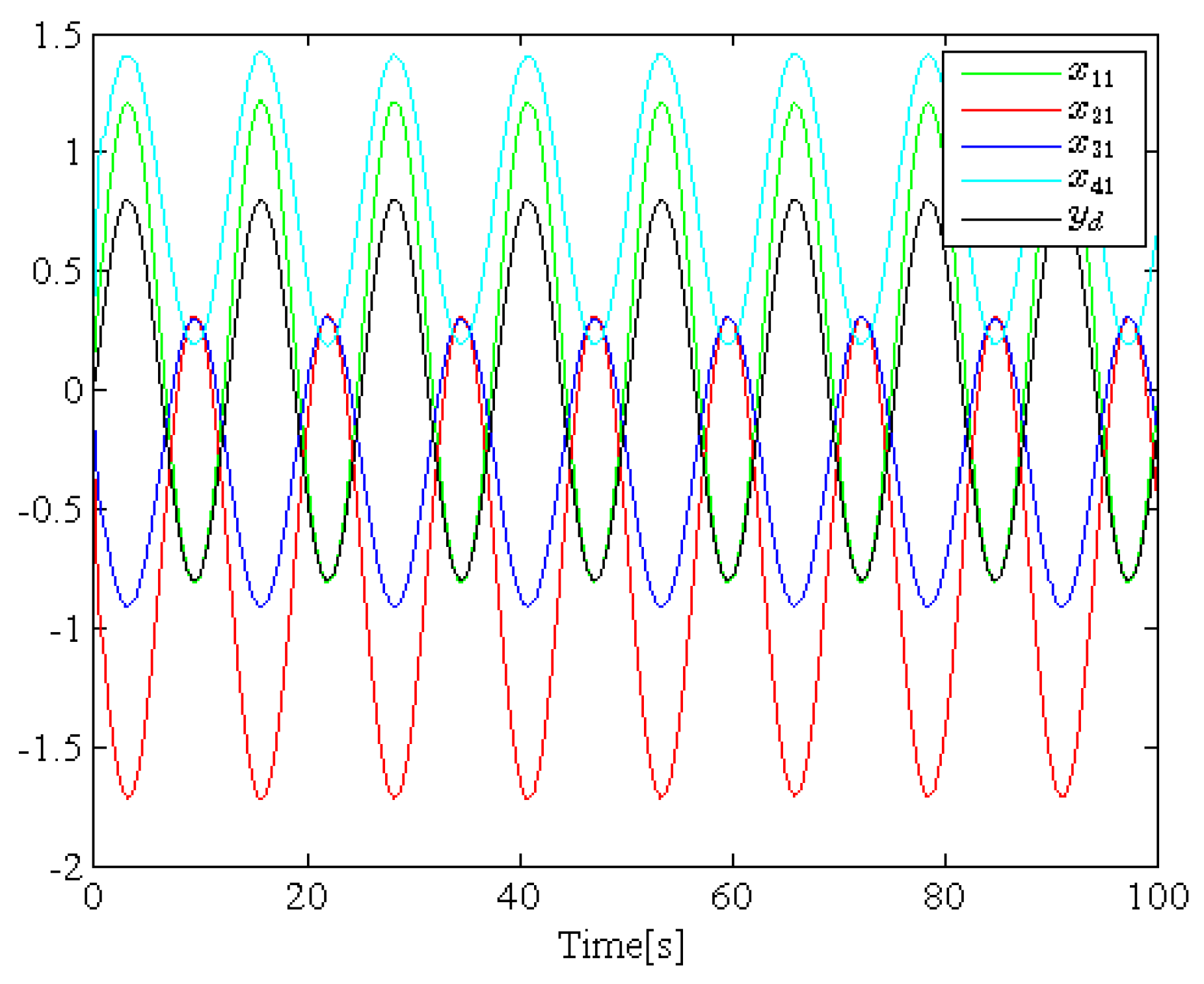
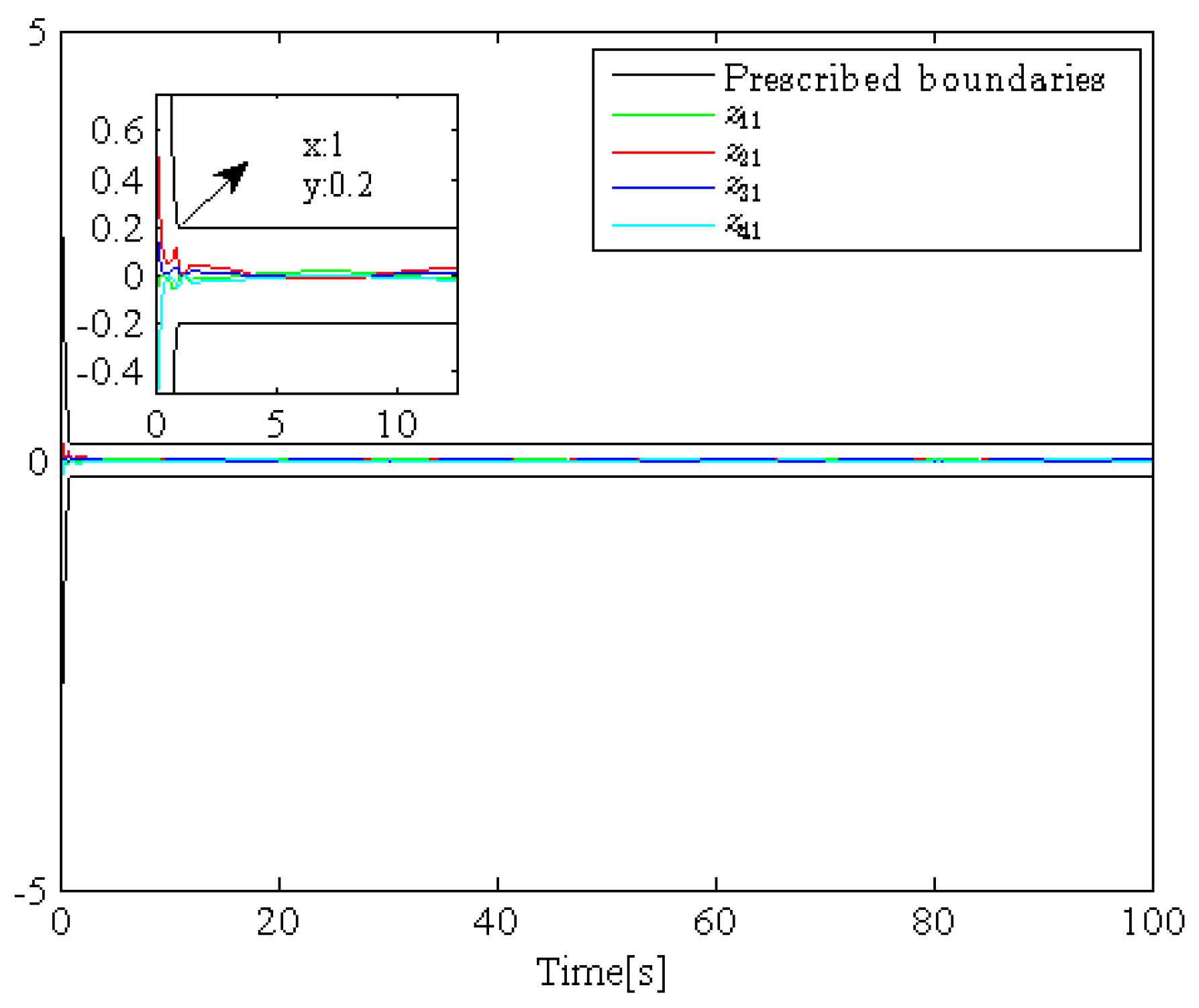
Bipartite formation consensus tracking control is realized, and the formation error converges to the prescribed boundary within a predesigned time $T_i$;

(2) 

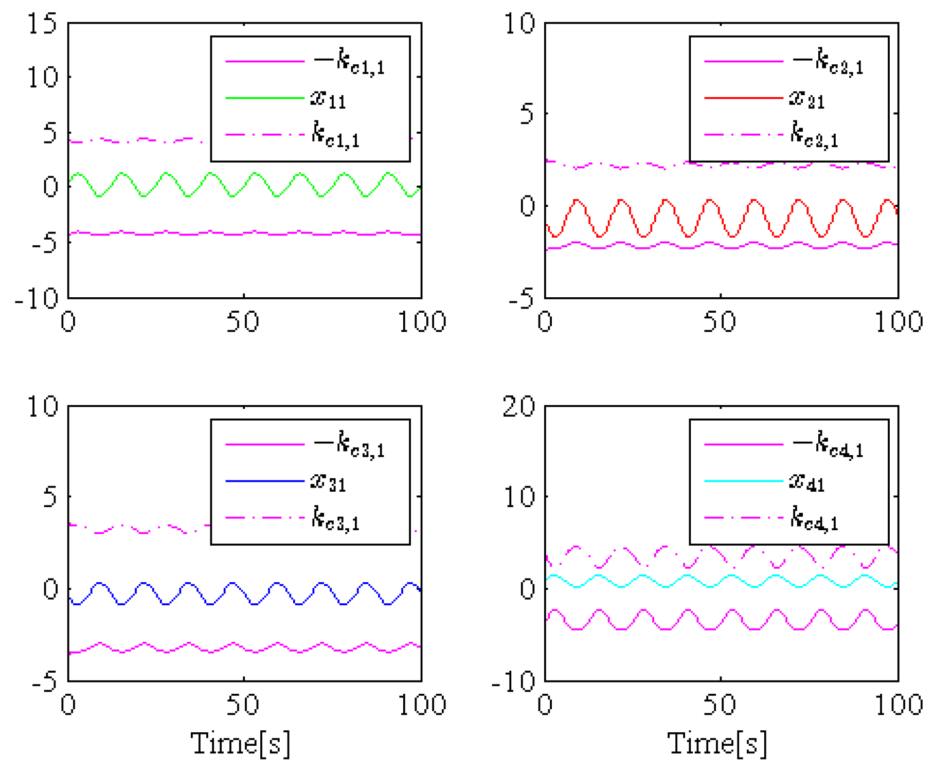
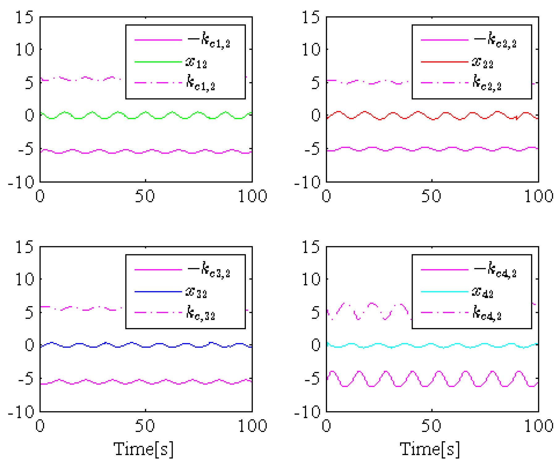
All states satisfy the constraint boundaries;

(3) 

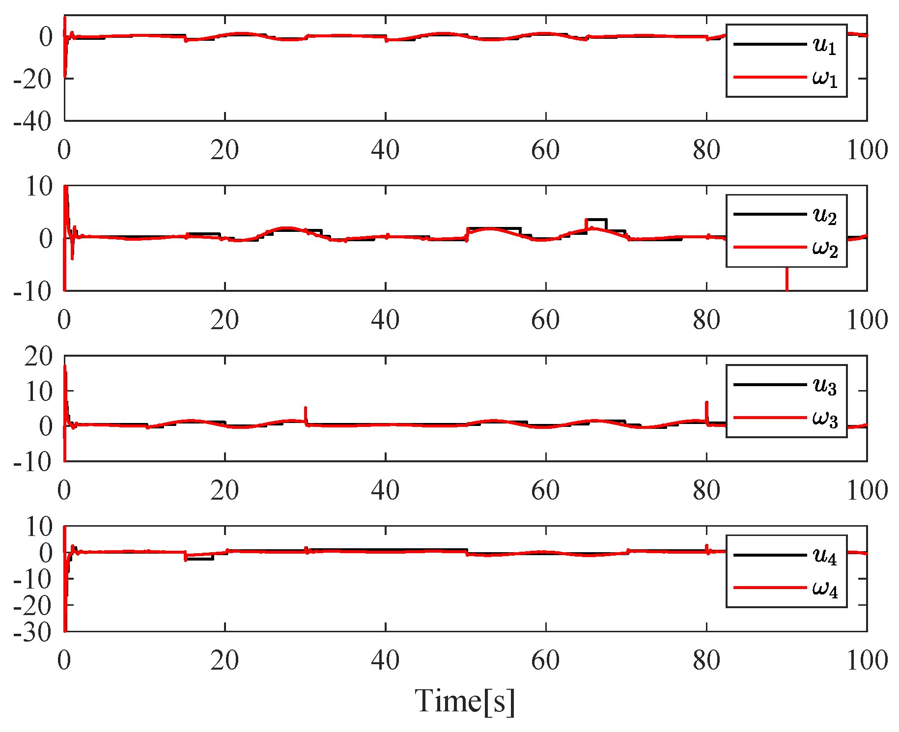
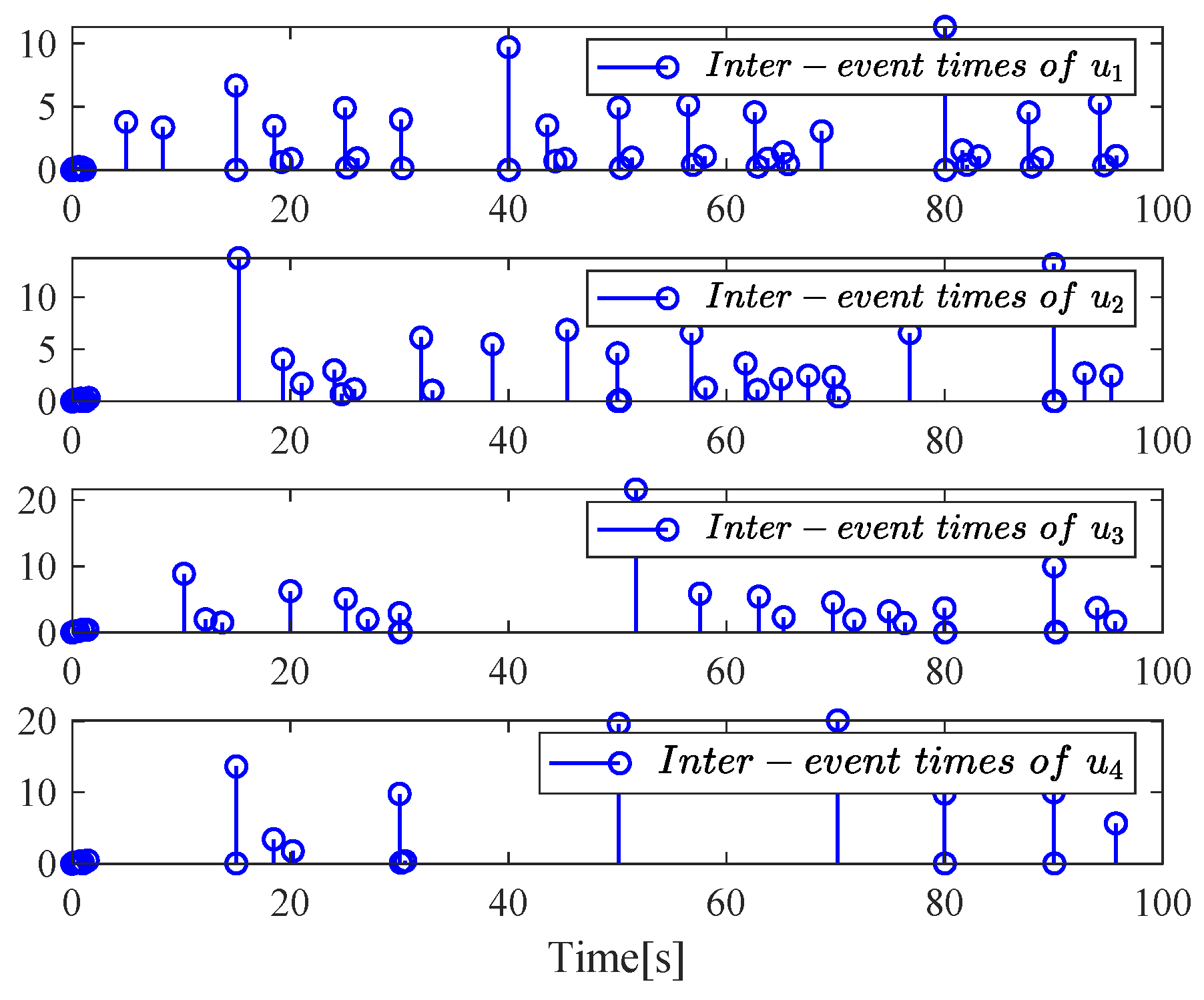
All signals are bounded with Zeno-free behavior.

Proof. 

Defining the overall BLF as $V={\displaystyle \sum _{\mathcal{l}=1}^S{V}_{\mathcal{l},S_{\mathcal{l}}}}$, we have:

$$\dot{V}\le {\displaystyle \sum _{\mathcal{l}=1}^S\left\{-{\displaystyle \sum _{q=1}^{S_{\mathcal{l}}}\frac{k_{\mathcal{l},q}{k}_{b\mathcal{l},q}^2\left({\overline{\chi }}_{\mathcal{l},q-1},t\right)}{\pi }\tan \left(\frac{\pi v_{\mathcal{l},q}^2}{2k_{b\mathcal{l},q}^2\left({\overline{\chi }}_{\mathcal{l},q-1},t\right)}\right)}\right.}\left.-{\displaystyle \sum _{q=1}^{S_{\mathcal{l}}}\frac{{\overline{\mu }}_{\mathcal{l},q}}{2{\mu }_{\mathcal{l},q}}{\tilde{\Theta }}_{\mathcal{l},q}^2+G_{\mathcal{l},S_{\mathcal{l}}}^k}\right\}\le -KV+G$$

(64)

where $K=\underset{\begin{array}{l}1\le \mathcal{l}\le S\\ 1\le p\le S_{\mathcal{l}}\end{array}}{\min }\left\{k_{\mathcal{l},q},{\overline{\mu }}_{\mathcal{l},q}\right\}$, $G=\underset{k\in {\Upsilon }_{\mathcal{l}}}{\max }{\displaystyle \sum _{\mathcal{l}=1}^S{G}_{\mathcal{l}}^k}$.

By multiplying both sides of inequality (64) by $e^{Kt}$ at the same time and integrating it on $\left[0,t\right]$, we have:

$$0\le V\left(t\right)\le e^{-Kt}V\left(0\right)+{\displaystyle \frac{G}{K}}\left(1-e^{-Kt}\right)$$

(65)

Based on (64) and (65), we have $\left|v_{\mathcal{l},q}\right|\le \left|k_{b\mathcal{l},q}\left({\overline{\chi }}_{\mathcal{l},q-1},t\right)\right|\sqrt{{\displaystyle \frac{2\arctan \left(G\pi /K{k}_{b\mathcal{l},q}^2\left({\overline{\chi }}_{\mathcal{l},q-1},t\right)\right)}{\pi }}}$, $\left|{\tilde{\Theta }}_{\mathcal{l},q}\right|\le \sqrt{2{\mu }_{\mathcal{l},q}\left(V\left(0\right)e^{-Kt}+G/K\right)}$. Based on the boundedness of $v_{\mathcal{l},q}$ and ${\tilde{\Theta }}_{\mathcal{l},q}$, it can be deduced that all signals are bounded.

We define ${\overline{k}}_{b\mathcal{l},q}\left({\overline{\chi }}_{\mathcal{l},q-1},t\right)=\left|k_{b\mathcal{l},q}\left({\overline{\chi }}_{\mathcal{l},q-1},t\right)\right|\sqrt{{\displaystyle \frac{2\arctan \left(G\pi /K{k}_{b\mathcal{l},q}^2\left({\overline{\chi }}_{\mathcal{l},q-1},t\right)\right)}{\pi }}}$. From (10) and (14), we have $\left|E_{\mathcal{l}}\left(t\right)\right|\le r_{\mathcal{l},1}+{\overline{k}}_{b\mathcal{l},1}\left({\overline{\chi }}_{\mathcal{l},0},t\right)$, and it follows that $\left|z_{\mathcal{l},1}\right|\le {\omega }_{\mathcal{l}}\left(t\right)$. According to [49], we have $\left|x_{\mathcal{l},q}^c-{\alpha }_{\mathcal{l},q}\right|\le {\kappa }_{\mathcal{l},q}$ and $\underset{t\to \infty }{\lim }\left|r_{\mathcal{l},q}\right|\le \sqrt{S_{\mathcal{l}}{\kappa }_{\mathcal{l}}^2/{\eta }_{\mathcal{l},0}}$, with ${\kappa }_{\mathcal{l}}=\max \left\{{\kappa }_{\mathcal{l},q},\right.\left.{\kappa }_{\mathcal{l},S_{\mathcal{l}}}\right\}$,${\eta }_{\mathcal{l},0}=$ $\min \left\{2k_{r\mathcal{l},1}-g_{\mathcal{l}}{\Psi }_{\mathcal{l}},\right.2\left(k_{r\mathcal{l},3}-{\displaystyle \frac{1}{2}}\right),2\left(k_{r\mathcal{l},2}-{\displaystyle \frac{1}{2}}\left(g_{\mathcal{l}}{\Psi }_{\mathcal{l}}-1\right)\right),$$\left.\cdots ,2\left(k_{r\mathcal{l},S_{\mathcal{l}}}-1\right)\right\}$. We define ${\overline{r}}_{\mathcal{l}}=\sqrt{{\displaystyle \frac{S_{\mathcal{l}}{\kappa }_{\mathcal{l}}^2}{{\eta }_{\mathcal{l},0}}}}$, and based on Lemma 3, we have $\left|e_{\mathcal{l}}\right|\le ‖e‖\le {\displaystyle \frac{‖z_1‖}{{\lambda }_{\min }\left(L+B\right)}}$; it follows that $\left|x_{\mathcal{l},1}\right|\le {\displaystyle \frac{‖z_1‖}{{\lambda }_{\min }\left(L+B\right)}}+Y_0\le {\displaystyle \frac{‖\omega \left(t\right)‖}{{\lambda }_{\min }\left(L+B\right)}}+Y_0$, with $\omega \left(t\right)={\left[{\omega }_1\left(t\right),\cdots ,{\omega }_S\left(t\right)\right]}^T$. Let $k_{\mathcal{l},1}\left({\overline{\chi }}_{\mathcal{l},0},t\right)=$ $Y_0+{\displaystyle \frac{‖\omega \left(t\right)‖}{{\lambda }_{\min }\left(L+B\right)}}$, and we have $\left|x_{\mathcal{l},1}\right|\le k_{\mathcal{l},1}\left({\overline{\chi }}_{\mathcal{l},0},t\right)$. Using the same process, we have $\left|x_{\mathcal{l},q}\right|=v_{\mathcal{l},q}+x_{\mathcal{l},q}^c+r_{\mathcal{l},q}\le$${\kappa }_{\mathcal{l},q}+k_{b\mathcal{l},q}\left({\overline{\chi }}_{\mathcal{l},q-1},t\right)+{\overline{\alpha }}_{\mathcal{l},q}+{\overline{r}}_{\mathcal{l}}$. Let $k_{\mathcal{l},q}\left({\overline{\chi }}_{\mathcal{l},q-1},t\right)={\kappa }_{\mathcal{l},q}+k_{b\mathcal{l},q}\left({\overline{\chi }}_{\mathcal{l},q-1},t\right)$ $+{\overline{\alpha }}_{\mathcal{l},q}+{\overline{r}}_{\mathcal{l}}$, and we have $\left|x_{\mathcal{l},q}\right|\le k_{\mathcal{l},q}\left({\overline{\chi }}_{\mathcal{l},q-1},t\right)$, $q=2,\cdots ,S_{\mathcal{l}}$. Based on the above discussion, all states are proved within the prescribed constraint boundaries.

As definition of the measurement error ${ħ}_{\mathcal{l}}\left(t\right)$ in (53), for $\forall t\in \left[t_{\mathcal{l},e},t_{\mathcal{l},e+1}\right)$, one has:

$${\displaystyle \frac{d}{dt}}\left|{ħ}_{\mathcal{l}}\right|=sign\left({ħ}_{\mathcal{l}}\right){\dot{ħ}}_{\mathcal{l}}\le \left|{\dot{\varpi }}_{\mathcal{l}}\right|$$

(66)

From (56), we can obtain ${\dot{\varpi }}_{\mathcal{l}}$, which is a differentiable and bounded signal in the closed-loop system. Thus, we have:

$$\left|{ħ}_{\mathcal{l}}\left(t\right)\right|={\displaystyle {\int }_{t_{\mathcal{l},e}}^{t_{\mathcal{l},e+1}}\left|{\dot{\varpi }}_{\mathcal{l}}\right|}dt\le {\displaystyle {\int }_{t_{\mathcal{l},e}}^{t_{\mathcal{l},e+1}}{W}_{\mathcal{l}}}dt\le W_{\mathcal{l}}\left(t_{\mathcal{l},e+1}-t_{\mathcal{l},e}\right)$$

(67)

where $W_{\mathcal{l}}>0$. It follows that:

$$\left(t_{\mathcal{l},e+1}-t_{\mathcal{l},e}\right)\ge {\displaystyle \frac{{\gamma }_{\mathcal{l}}\left|{\varpi }_{\mathcal{l}}\left(t\right)\right|+m_{\mathcal{l}}}{W_{\mathcal{l}}}}>0$$

(68)

It can be deduced from (68) that the Zeno behavior can be ruled out. The proof of Theorem 1 is complete.□

4. Simulation Example

An MAS consisting of four followers and one leader is considered to illustrate the effectiveness of the control method. The directed graph is shown in Figure 1.

The dynamic of the $\mathcal{l}$-th follower is described as:

$$\begin{gathered} {\dot{x}}_{\mathcal{l},1}=x_{\mathcal{l},2}+f_{\mathcal{l},1}^{{\sigma }_{\mathcal{l}}\left(t\right)}\left(x_{\mathcal{l},1}\right) \\ {\dot{x}}_{\mathcal{l},2}=u_{\mathcal{l}}+f_{\mathcal{l},2}^{{\sigma }_{\mathcal{l}}\left(t\right)}\left({\overline{x}}_{\mathcal{l},2}\right) \\ {y}_{\mathcal{l}}=x_{\mathcal{l},1},\mathcal{l}=1,2,3,4 \end{gathered}$$

(69)

where ${\sigma }_{\mathcal{l}}\left(t\right)\in {\Upsilon }_{\mathcal{l}}=\left\{1,2\right\}$. The unknown functions are chosen as $f_{\mathcal{l},1}^1=0.1\sin (x_{\mathcal{l}.1})$, $f_{\mathcal{l},1}^2=0.1x_{\mathcal{l},1}^2$, $f_{\mathcal{l},2}^1=0.1\sin (x_{\mathcal{l},1})x_{\mathcal{l},2}$, and $f_{\mathcal{l},2}^2=x_{\mathcal{l},1}+0.1x_{\mathcal{l},2}$. The leader signal is chosen as $y_r=0.8\sin (0.5t)$.

The expected formation functions are chosen as: ${\delta }_1\left(t\right)=0.2+0.2\sin \left(0.5t\right)$, ${\delta }_2\left(t\right)=0.2\sin (0.5t)-0.3$, ${\delta }_3\left(t\right)=0.2\sin (0.5t)-0.3$, and ${\delta }_4\left(t\right)=0.2\sin (0.5t)+0.2$.

The FTPPF is defined as:

$${\omega }_{\mathcal{l}}\left(t\right)=\left\{\begin{array}{ll}{\left({\omega }_{\mathcal{l},0}^{h_{\mathcal{l}}}-h_{\mathcal{l}}{\tau }_{\mathcal{l}}t\right)}^{1/h_{\mathcal{l}}}+{\omega }_{\mathcal{l},T_{\mathcal{l}}},& t<T_{\mathcal{l}}\\ {\omega }_{\mathcal{l},T_{\mathcal{l}}},& t\ge T_{\mathcal{l}}\end{array}\right.$$

where ${\omega }_{\mathcal{l},0}=4$, ${\omega }_{\mathcal{l},T_{\mathcal{l}}}=0.2$, ${\tau }_{\mathcal{l}}=4$, $d_{\mathcal{l}}=10$, ${\vartheta }_{\mathcal{l}}=5$. Then, $h_{\mathcal{l}}=0.5$, and the setting time $T_{\mathcal{l}}=1$,$\mathcal{l}=1,2,3,4$.

The fuzzy membership function is chosen as:

$${\mu }_{F_{\mathcal{l},q}^{\iota }}\left(x_{\mathcal{l},q}\right)=\exp \left(-{\displaystyle \frac{{\left(x_{\mathcal{l},q}-4+2\iota \right)}^2}{8}}\right), \mathcal{l}=1,2,3,4, q=1,2, \iota =1,2,3,4,5.$$

The function constraints on states are designed as:

$$\begin{gathered} k_{c1,1}\left({\overline{x}}_{1,0},t\right)=e^{-0.2y_d}+e^{-2t}+3.5, k_{c1,2}\left({\overline{\chi }}_{1,1},t\right)=e^{-0.1x_{1,1}}+e^{-0.2y_d}+e^{-2t}+4.5; \\ {k}_{c2,2}\left({\overline{\chi }}_{2,1},t\right)=e^{-0.1x_{2,1}}-e^{-0.2y_d}+e^{-2t}+4.5; k_{c3,1}\left({\overline{x}}_{3,0},t\right)=-e^{-0.4y_1}+e^{-0.2y_d}+e^{-2t}+3.2, \\ {k}_{c3,2}\left({\overline{\chi }}_{3,1},t\right)=e^{-0.1x_{3,1}}-e^{-0.4y_1}+e^{-0.2y_d}+e^{-2t}+4.5; k_{c4,1}\left({\overline{x}}_{4,0},t\right)=-e^{-0.6y_2}+e^{-0.2y_d}+e^{-2t}+3.2, \\ {k}_{c4,2}\left({\overline{\chi }}_{4,1},t\right)=e^{-0.1x_{4,1}}-e^{-0.6y_2}+e^{-0.2y_d}+e^{-2t}+4.5 \end{gathered}$$

Relevant design parameters are selected: ${\mu }_{\mathcal{l},q}=1$, ${\overline{\mu }}_{\mathcal{l},q}=0.01$, ${\iota }_{\mathcal{l},1}={\iota }_{\mathcal{l},2}=1$, ${\gamma }_{\mathcal{l}}=0.5$, ${ƛ}_{\mathcal{l}}=10$, $c_{\mathcal{l},1}=20$, $c_{\mathcal{l},2}=15$, $m_1=0.4$, $m_2=m_3=0.5$, $m_4=0.8$, ${\overline{m}}_{\mathcal{l}}=2$, ${ħ}_{\mathcal{l},1}=15$, ${ħ}_{\mathcal{l},2}=30$, ${\varphi }_{\mathcal{l},q}=370$, and ${\xi }_{\mathcal{l},q}=0.7$ ($\mathcal{l}=1,2,3,4$, $q=1,2$).

The corresponding initial condition is chosen: ss, $x_{\mathcal{l},2}\left(0\right)=0.01$, and the rest are chosen as 0.

The simulation responses are shown as Figure 2, Figure 3, Figure 4, Figure 5, Figure 6, Figure 7 and Figure 8. Figure 2 shows the switching dynamic of four followers. Figure 3 shows the trajectories of the control input and adaptive controller of each follower. Figure 4 exhibits the control input-triggered time sequence for each follower. Figure 5 demonstrates the time-varying formation behaviors of agents. The formation errors of four followers and the prescribed boundary curves are shown in Figure 6. The followers’ state variables and the function constraints on states are shown in Figure 7 and Figure 8.

Furthermore, according to Figure 4, the cumulative triggering times of each follower control input in the time interval [0, 100] can be calculated as follows: Agent 1: 53 times, Agent 2: 49 times, Agent 3: 34 times, and Agent 4: 24 times. In a total of 1000 samples, the sampling rates of each follower were 5.3%, 4.9%, 3.4%, and 2.4%, respectively. Therefore, by introducing the ETC strategy, the control input update times and sampling rates were significantly reduced, thereby saving communication and computational burdens, and no Zeno behavior occurred. According to Figure 5 and Figure 6, it can be seen that the bipartite formation consensus tracking control was realized, and the formation error converged to the prescribed performance boundary within the setting time $T_{\mathcal{l}}=1s$. It can be concluded from Figure 7 and Figure 8 that all state variables were within the functional constraints on states. It turns out that all signals were bounded, and the previously mentioned control objectives could be achieved.

Remark 2.

Firstly, the formation error is defined so that all followers meet the expected formation. Secondly, the FTPPT function is designed to ensure that the formation error converges to the prescribed performance boundary within a predefined time. Thirdly, the “explosion of complexity” problem is solved by introducing a command filter. Fourthly, the barrier Lyapunov function is constructed to solve the problem of function constraints on states. Subsequently, the ETC mechanism is introduced to balance communication load and system performance. Finally, based on the stability theory of the common Lyapunov stability theory, it is proven that all signals are bounded.

5. Conclusions

An adaptive distributed fuzzy event-triggered FTTP bipartite formation tracking control has been investigated for switched nonlinear MASs with function constraints on states. Both formation error constraints and state constraints were warranted by introducing the FTPPF and constructing the tan-type BLF. On the basis of an integrated backstepping control and command filter, as well as the introduced ETC strategy, an event-triggered bipartite formation tracking control scheme has been proposed. It has been proven that the problem of the explosion of complexity was eliminated, the communication pressure was released, and the functional state constraints were handled; meanwhile, the stability of the system was ensured and bipartite formation tracking control was realized. Finally, the feasibility and effectiveness of the control scheme were proven through the simulation example.

Although the control objectives have been achieved, there are still some conservative issues that need to be improved. Specifically, this study only considers the convergence time and transient performance of the formation error, while ignoring the rapid convergence of other signals. Considering the above conservative issues, extending the proposed control scheme to finite-time control [55,56] is a meaningful and worthy research topic.

References

1. Gao, X.Y.; Wang, J.Q.; Teo, K.L.; Yang, H.F.; Yang, X.R. Dynamic gain scheduling control design for linear multiagent systems subject to input saturation. J. Frankl. Inst. 2023, 360, 4597–4625. [Google Scholar] [CrossRef]
2. Wang, Z.H. Consensus control for linear multiagent systems under delayed transmitted information. IEEE Trans. Syst. Man Cybern. Syst. 2023, 53, 5670–5678. [Google Scholar] [CrossRef]
3. Wu, J.; Lu, M.; Deng, F.; Chen, J. Cooperative Output Regulation of Heterogeneous Linear Multi-Agent Systems: A Distributed Output Feedback Control Approach. In Proceedings of the 2023 China Automation Congress (CAC), Chongqing, China, 17–19 November 2023; pp. 5112–5117. [Google Scholar]
4. Ma, Z.; Tong, S. Nonlinear filters-based adaptive fuzzy control of strict-feedback nonlinear systems with unknown asymmetric dead-zone output. IEEE Trans. Autom. Sci. Eng. 2024, 21, 5099–5109. [Google Scholar] [CrossRef]
5. Yu, J.; Shi, P.; Dong, W.; Lin, C. Adaptive fuzzy control of nonlinear systems with unknown dead zones based on command filtering. IEEE Trans. Fuzzy Syst. 2018, 26, 46–55. [Google Scholar] [CrossRef]
6. Wang, H.; Zong, G.; Yang, D.; Xia, J. Observer-based adaptive neural fault-tolerant control for nonlinear systems with prescribed performance and input dead-zone. Int. J. Robust Nonlinear Control. 2024, 34, 114–131. [Google Scholar] [CrossRef]
7. Zhou, R.; Wen, G.; Zhu, J.; Li, B. Adaptive neural network observer control for a class of nonlinear strict-feedback systems with unmeasurable states. Int. J. Control. 2024, 97, 165–174. [Google Scholar] [CrossRef]
8. Chen, L.; Tong, S. Observer-based adaptive fuzzy consensus control of nonlinear multi-agent systems encountering deception attacks. IEEE Trans. Ind. Inform. 2024, 20, 1808–1818. [Google Scholar] [CrossRef]
9. Liu, Z.; Huang, H.; Park, J.H.; Huang, J.; Wang, X.; Lv, M. Adaptive fuzzy control for unknown nonlinear multi-agent systems with switching directed communication topologies. IEEE Trans. Fuzzy Syst. 2023, 31, 2487–2494. [Google Scholar] [CrossRef]
10. Liu, D.; Liu, Z.; Chen, C.L.P.; Zhang, Y. Distributed adaptive neural control for uncertain multi-agent systems with unknown actuator failures and unknown dead zones. Nonlinear Dyn. 2020, 99, 1001–1017. [Google Scholar] [CrossRef]
11. Chen, L.; Li, Y.; Tong, S. Neural network adaptive consensus control for nonlinear multi-agent systems encountered sensor attacks. Int. J. Syst. Sci. 2023, 54, 2536–2550. [Google Scholar] [CrossRef]
12. Caiazzo, B.; Lui, D.G.; Petrillo, A.; Santini, S. Signed average consensus in cooperative-antagonistic multi-agent systems with multiple communication time-varying delays. IFAC-Pap. 2024, 58, 114–119. [Google Scholar] [CrossRef]
13. Zhao, M.; Peng, C.; Tian, E. Finite-time and fixed-time bipartite consensus tracking of multi-agent systems with weighted antagonistic interactions. IEEE Trans. Circuits Syst. I Regul. Pap. 2021, 68, 426–433. [Google Scholar] [CrossRef]
14. Gong, X.; Cui, Y.; Shen, J.; Shu, Z.; Huang, T. Distributed prescribed-time interval bipartite consensus of multi-agent systems on directed graphs: Theory and experiment. IEEE Trans. Netw. Sci. Eng. 2021, 8, 613–624. [Google Scholar] [CrossRef]
15. Wang, L.; Yan, H.; Chang, Y.; Wang, M.; Li, Z. Fixed-time fully distributed observer-based bipartite consensus tracking for nonlinear heterogeneous multiagent systems. Inf. Sci. 2023, 635, 221–235. [Google Scholar] [CrossRef]
16. Liu, D.; Zhou, Z.P.; Li, T.S. Data-driven bipartite consensus tracking for nonlinear multiagent systems with prescribed performance. IEEE Trans. Syst. Man Cybern. Systems 2023, 53, 3666–3674. [Google Scholar] [CrossRef]
17. Vamvoudakis, K.G. Event-triggered optimal adaptive control algorithm for continuous-time nonlinear systems. IEEE/CAA J. Autom. Sin. 2014, 1, 282–293. [Google Scholar] [CrossRef]
18. Yang, Y.; Niu, Y. Event-triggered adaptive neural backstepping control for nonstrict-feedback nonlinear time-delay systems. J. Frankl. Inst. 2020, 357, 4624–4644. [Google Scholar] [CrossRef]
19. Ning, P.; Hua, C.; Li, K.; Meng, R. Event-triggered control for nonlinear uncertain systems via a prescribed-time approach. IEEE Trans. Autom. Control. 2023, 68, 6975–6981. [Google Scholar] [CrossRef]
20. Zhang, J.; Niu, B.; Wang, D.; Wang, H.; Zhao, P.; Zong, G. Time-/event-triggered adaptive neural asymptotic tracking control for nonlinear systems with full-state constraints and application to a single-link robot. IEEE Trans. Neural Netw. Learn. Syst. 2022, 33, 6690–6700. [Google Scholar] [CrossRef]
21. Ren, H.; Liu, R.; Cheng, Z.; Ma, H.; Li, H. Data-driven event-triggered control for nonlinear multi-agent systems with uniform quantization. IEEE Trans. Circuits Syst. II: Express Briefs 2024, 71, 712–716. [Google Scholar] [CrossRef]
22. Yang, X.; Zhang, X.; Cao, J.; Liu, H. Observer-based adaptive fuzzy fractional backstepping consensus control of uncertain multiagent systems via event-triggered scheme. IEEE Trans. Fuzzy Syst. 2024, 32, 3953–3967. [Google Scholar] [CrossRef]
23. Chen, X.; Hu, S.; Yang, T.; Xie, X.; Qiu, J. Event-triggered bipartite consensus of multiagent systems with input saturation and DoS attacks over weighted directed networks. IEEE Trans. Syst. Man Cybern. Syst. 2024, 54, 4054–4065. [Google Scholar] [CrossRef]
24. Zhang, W.; Huang, Q.; Alhudhaif, A. Event-triggered fixed-time bipartite consensus for nonlinear disturbed multi-agent systems with leader-follower and leaderless controller. Inf. Sci. 2024, 662, 120243. [Google Scholar] [CrossRef]
25. Zhou, H.; Tong, S. Fuzzy adaptive event-triggered resilient formation control for nonlinear multiagent systems under DoS attacks and input saturation. IEEE Trans. Syst. Man Cybern. Syst. 2024, 54, 3665–3674. [Google Scholar] [CrossRef]
26. Yang, W.; Shi, Z.; Zhong, Y. Robust time-varying formation control for uncertain multi-agent systems with communication delays and nonlinear couplings. Int. J. Robust Nonlinear Control. 2024, 34, 147–166. [Google Scholar] [CrossRef]
27. Yang, S.; Bai, W.; Li, T.; Shi, Q.; Yang, Y.; Wu, Y.; Chen, C.P. Neural-network-based formation control with collision, obstacle avoidance and connectivity maintenance for a class of second-order nonlinear multi-agent systems. Neurocomputing 2021, 439, 243–255. [Google Scholar] [CrossRef]
28. Valcher, M.; Misra, P. On the consensus and bipartite consensus in high-order multi-agent dynamical systems with antagonistic interactions. Syst. Control. Lett. 2014, 66, 94–103. [Google Scholar] [CrossRef]
29. Cai, Y.; Zhang, H.; Gao, Z.; Yang, L.; He, Q. Adaptive bipartite event-triggered time-varying output formation tracking of heterogeneous linear multi-agent systems under signed directed graph. IEEE Trans. Neural Netw. Learn. Syst. 2022, 34, 7049–7058. [Google Scholar] [CrossRef]
30. Cai, Y.; Zhang, H.; Zhang, J.; Xi, R.; He, Q. Fully distributed bipartite time-varying formation control for uncertain linear multi-agent systems under event-triggered mechanism. Int. J. Robust Nonlinear Control. 2021, 31, 5165–5187. [Google Scholar] [CrossRef]
31. Lu, W.; Zong, C.; Li, J.; Liu, D. Bipartite consensus-based formation control of high-order multi-robot systems with time-varying delays. Trans. Inst. Meas. Control. 2022, 44, 1297–1308. [Google Scholar] [CrossRef]
32. Li, W.; Zhang, H.; Zhou, Y.; Wang, Y. Bipartite formation tracking for multi-agent systems using fully distributed dynamic edge-event-triggered protocol. IEEE/CAA J. Autom. Sinica 2022, 9, 847–853. [Google Scholar] [CrossRef]
33. Li, W.; Zhang, H.; Cai, Y.; Wang, Y. Fully distributed event-triggered bipartite formation tracking for multi-agent systems with multiple leaders and matched uncertainties. Inf. Sci. 2022, 596, 537–550. [Google Scholar] [CrossRef]
34. Zhao, Y.; Zhu, F.; Xu, D. Self-triggered bipartite formation-containment control for heterogeneous multi-agent systems with disturbances. Neurocomputing 2023, 548, 126382. [Google Scholar] [CrossRef]
35. Li, T.; Li, S.; Wang, Y.; Hui, Y.; Han, J. Bipartite Formation Control of Nonlinear Multi-Agent Systems with Fixed and Switching Topologies under Aperiodic DoS Attacks. Electronics 2024, 13, 696. [Google Scholar] [CrossRef]
36. Wang, X.; Ye, D.; Wei, F. Optimized bipartite formation control for multiagent systems with obstacle and collision avoidance. Inf. Sci. 2024, 662, 120122. [Google Scholar] [CrossRef]
37. Chen, Z.; Liu, Y.; He, W.; Qiao, H.; Ji, H. Adaptive-neural-network-based trajectory tracking control for a nonholonomic wheeled mobile robot with velocity constraints. IEEE Trans. Ind. Electron. 2021, 68, 5057–5067. [Google Scholar] [CrossRef]
38. Li, D.; Wang, Y.; Liu, Y.J.; Liu, L. IBLFs-based adaptive fuzzy control for Continuous Stirred Tank Reactors with full state constraints and actuator faults. J. Process Control. 2023, 124, 14–24. [Google Scholar] [CrossRef]
39. Wang, J.; Yan, Y.; Liu, Z.; Chen, C.P.; Zhang, C.; Chen, K. Finite-time consensus control for multi-agent systems with full-state constraints and actuator failures. Neural Netw. 2023, 157, 350–363. [Google Scholar] [CrossRef] [PubMed]
40. Sun, L.; Zang, Y.; Zhang, X.; Zhu, G.; Zhong, C.; Wang, C. Adaptive event-triggered cooperative tracking control under full-state constraints based on nonlinear time-varying multi-agent systems. Int. J. Control Autom. Syst. 2024, 22, 867–882. [Google Scholar] [CrossRef]
41. Sui, J.; Liu, C.; Niu, B.; Zhao, X.; Wang, D.; Yan, B. Prescribed performance adaptive containment control for full-state constrained nonlinear multiagent systems: A disturbance observer-based design strategy. IEEE Trans. Autom. Sci. Eng. 2024, 1–12. [Google Scholar] [CrossRef]
42. Wang, X.; Pang, N.; Xu, Y.; Huang, T.; Kurths, J. On state-constrained containment control for nonlinear multiagent systems using event-triggered input. IEEE Trans. Syst. Man Cybern. Syst. 2024, 54, 2530–2538. [Google Scholar] [CrossRef]
43. Shahvali, M.; Azarbahram, A.; Naghibi-Sistani, M.B.; Askari, J. Bipartite consensus control for fractional-order nonlinear multi-agent systems: An output constraint approach. Neurocomputing 2020, 397, 212–223. [Google Scholar] [CrossRef]
44. Huang, S.; Zong, G.; Niu, B.; Xu, N.; Zhao, X. Dynamic self-triggered fuzzy bipartite time-varying formation tracking for nonlinear multiagent systems with deferred asymmetric output constraints. IEEE Trans. Fuzzy Syst. 2024, 32, 2700–2712. [Google Scholar] [CrossRef]
45. Sui, S.; Shen, D.; Bi, W.; Tong, S.; Chen, C.L.P. Observer-based event-triggered bipartite consensus for nonlinear multi-agent systems: Asymmetric full-state constraints. IEEE Trans. Autom. Sci. Eng. 2024, 1–11. [Google Scholar] [CrossRef]
46. Niu, B.; Zhang, Y.; Zhao, X.; Wang, H.; Sun, W. Adaptive predefined-time bipartite consensus tracking control of constrained nonlinear MASs: An improved nonlinear mapping function method. IEEE Trans. Cybern. 2023, 53, 6017–6026. [Google Scholar] [CrossRef] [PubMed]
47. Liu, S.; Niu, B.; Karimi, H.R.; Zhao, X. Self-triggered fixed-time bipartite fault-tolerant consensus for nonlinear multiagent systems with function constraints on states. Chaos Soliton. Fract. 2024, 178, 114367. [Google Scholar] [CrossRef]
48. Xin, B.; Cheng, S.; Wang, Q.; Chen, J.; Deng, F. Fixed-time prescribed performance consensus control for multiagent systems with nonaffine faults. IEEE Trans. Fuzzy Syst. 2023, 31, 3433–3446. [Google Scholar] [CrossRef]
49. Bi, W.; Zhang, C.; Sui, S.; Tong, S.; Chen, C.P. Fixed-Time Fuzzy Adaptive Bipartite Output Consensus Tracking for Nonlinear Coopetition MASs. IEEE Trans. Fuzzy Syst. 2024, 32, 2775–2785. [Google Scholar] [CrossRef]
50. Li, X.; Long, L. Distributed event-triggered fuzzy control of heterogeneous switched multiagent systems under Switching topologies. IEEE Trans. Fuzzy Syst. 2024, 32, 574–585. [Google Scholar] [CrossRef]
51. Niu, B.; Liu, X.; Guo, Z.; Jiang, H.; Wang, H. Adaptive intelligent control-based consensus tracking for a class of switched nonstrict feedback nonlinear multiagent systems with unmodeled dynamics. IEEE Trans. Artif. Intell. 2024, 5, 1624–1634. [Google Scholar] [CrossRef]
52. Zhang, R.; Li, S.; Ahn, C.K.; Chadli, M. Fully distributed adaptive fuzzy consensus for heterogeneous switched nonlinear multiagent systems under state-dependent switchings. IEEE Trans. Fuzzy Syst. 2024, 32, 607–620. [Google Scholar] [CrossRef]
53. Liang, H.; Wang, W.; Pan, Y.; Lam, H.K.; Sun, J. Synchronous MDADT-based fuzzy adaptive tracking control for switched multiagent systems via modified self-triggered mechanism. IEEE Trans. Fuzzy Syst. 2024, 32, 2876–2889. [Google Scholar] [CrossRef]
54. Yoo, S.J.; Park, B.S. Adaptive flexible performance function approach for dynamic obstacle avoidance to distributed formation tracking of range-constrained switched nonlinear multiagent systems. Int. J. Robust Nonlinear Control. 2024, 34, 4864–4880. [Google Scholar] [CrossRef]
55. Li, Y.; Li, Y.; Tong, S. Event-based finite-time control for nonlinear multiagent systems with asymptotic tracking. IEEE Trans. Autom. Control. 2023, 68, 3790–3797. [Google Scholar] [CrossRef]
56. Andreotti, A.; Caiazzo, B.; Lui, D.; Petrillo, A.; Santini, S. Asymptotic voltage restoration in islanded microgrids via an adaptive asynchronous event-triggered finite-time fault-tolerant control. Sustain. Energy Grids Netw. 2024, 39, 101406. [Google Scholar] [CrossRef]
Figure 1. Communication graph topology.
Actuators 14 00023 g001
Figure 2. The trajectory of switching signal σ l ( t ) ( l = 1 , 2 , 3 , 4 ).
Actuators 14 00023 g002
Figure 3. Adaptive controller ϖ l and control input u l , l = 1 , 2 , 3 , 4 .
Actuators 14 00023 g003
Figure 4. Inter-event times of control inputs.
Actuators 14 00023 g004
Figure 5. Time-varying formation behaviors of agents.
Actuators 14 00023 g005
Figure 6. Curve of formation error z l , 1 , l = 1 , 2 , 3 , 4 .
Actuators 14 00023 g006
Figure 7. Follower state vectors x l , 1 and the constraint boundary k l , 1 χ ¯ l , 0 , t .
Actuators 14 00023 g007
Figure 8. Follower state vector x l , 2 and the constraint boundary k l , 2 χ ¯ l , 1 , t .
Actuators 14 00023 g008
Disclaimer/Publisher’s Note: The statements, opinions and data contained in all publications are solely those of the individual author(s) and contributor(s) and not of MDPI and/or the editor(s). MDPI and/or the editor(s) disclaim responsibility for any injury to people or property resulting from any ideas, methods, instructions or products referred to in the content.