Article

Deep Reinforcement Learning-Based Enhancement of Robotic Arm Target-Reaching Performance

by
Ldet Honelign
1,†,‡,
Yoseph Abebe
1,‡,
Abera Tullu
2,‡ and
Sunghun Jung
2,*
1
Department of Electromechanical Engineering, Addis Ababa Science and Technology University, Kilnto 16417, Ethiopia
2
Faculty of Smart Vehicle System Engineering, Chosun University, Dong-gu, Gwangju 61452, Republic of Korea
*
Author to whom correspondence should be addressed.
Current address: Department of Aerospace Engineering, Chosun University, Seoseok-dong, Gwangju 61452, Republic of Korea.
These authors contributed equally to this work.
Actuators 2025, 14(4), 165; https://doi.org/10.3390/act14040165
Submission received: 25 January 2025 / Revised: 12 March 2025 / Accepted: 21 March 2025 / Published: 26 March 2025
(This article belongs to the Special Issue From Theory to Practice: Incremental Nonlinear Control)

Abstract

:
This work investigates the implementation of the Deep Deterministic Policy Gradient (DDPG) algorithm to enhance the target-reaching capability of the seven degree-of-freedom (7-DoF) Franka Pandarobotic arm. A simulated environment is established by employing OpenAI Gym, PyBullet, and Panda Gym. After 100,000 training time steps, the DDPG algorithm attains a success rate of 100% and an average reward of −1.8. The actor loss and critic loss values are 0.0846 and 0.00486, respectively, indicating improved decision-making and accurate value function estimations. The simulation results demonstrate the efficiency of DDPG in improving robotic arm performance, highlighting its potential for application to improve robotic arm manipulation.

1. Introduction

Enhancing the precision of robotic arm manipulation remains a core research area towards the aim of achieving full autonomy of robots in various sectors such as industrial manufacturing and assembly processes. given the maturity of image recognition and vision systems, the next logical progression in this field is to achieve complete autonomy of robotic manipulators through the use of machine learning (ML), artificial neural networks (ANNs), and artificial intelligence (AI) as a whole [1,2]. Numerous attempts have been made to create intelligent robots that can take tasks and execute them accordingly [3,4,5,6,7,8,9,10].
Although the development of a system with intelligence close to that of humans is still a long way off, robots that can perform specialized autonomous activities such as intelligent facial emotion recognition [11], flying in natural and man-made environments [12], driving a vehicle [13], swimming [14], carrying boxes and materials over different terrains [15], and picking up and placing objects [16,17] have already been realized.
However, some challenges must be overcome in order to achieve this goal. For instance, the mapping complexity from Cartesian space to the joint space of a robotic arm increases with the number of joints and linkages possessed by the manipulator. This is problematic, as the tasks assigned to a robotic arm are in Cartesian space, whereas the commands (velocity or torque) are in joint space [18,19]. Therefore, if full autonomy of robotic manipulators is the objective, then resolving the target-reaching problem represents one of the most crucial factors that must be addressed.
As described in [20,21], reinforcement learning is a type of machine learning that aims to maximize the outcome of a given system by using a dynamic and autonomous trial-and-error approach. It shares a similar objective with human intelligence, which is characterized by the ability to perceive and retain information as knowledge to be used for environment-adaptive behaviors. Trial-and-error search and delayed rewards are fundamental aspects of reinforcement leaning, which allows the learning strategy to interact with the environment by performing actions and discovering rewards [22]. Through this approach, software agents and machines can automatically select the most effective course of action to take in a given circumstance, resulting in improved performance. Reinforcement learning offers a framework and set of tools for designing sophisticated and complex robotic behaviors [23,24]. In contrast, the challenges presented by robotic issues serve as motivation, impact, and confirmation of advances in reinforcement learning. Multiple previous works on the implementation of reinforcement learning in the field of robotics depict this fact [25,26,27,28,29].
In addition to the above-mentioned studies, several different approaches to robotic manipulation have been investigated, including model-based reinforcement learning [30], supervised learning-based approaches [31], and classical control-based techniques. Although these techniques have proven effective in various settings, they often come with limitations in terms of flexibility, sample efficiency, or generalization to unseen tasks. In contrast, the proposed method makes use of reinforcement learning to improve robotic manipulators’ capacity for self-adaptation to changing surroundings. Instead of depending only on preset models or rules, reinforcement learning allows robots to learn from their experiences and improve their performance. This paper further examines the performance of our approach compared to existing reinforcement learning methods in terms of efficiency, stability, and real-world applicability.
Recent advances in RL-based robotic manipulation have focused on improving sampling efficiency, stability, and real-world generalization. The Soft Actor–Critic (SAC) algorithm is a model-free deep reinforcement learning algorithm capable of handling continuous action spaces, and has shown strong adaptability in domains such as energy-efficient building control, where it achieved a 9.7% reduction in energy costs while maintaining thermal comfort [32]. Similarly, Twin Delayed DDPG (TD3) has been improved through priority experience replay and transfer learning, significantly improving learning efficiency in mobile robot path planning, as demonstrated by increasing success rates by 16.6% and reducing training times by 23.5% [33].
Although model-based approaches such as PILCO [34] offer superior sample efficiency, they often struggle with high-dimensional control problems such as robotic manipulation. In contrast, policy-gradient methods such as PPO and DDPG remain widely used thanks to their direct interaction-based learning capabilities. However, challenges such as hyperparameter sensitivity and the exploration–exploitation tradeoff continue to persist, representing critical areas of research.
The key contributions of this work are as follows:
  • Implementation of the deep deterministic policy gradient algorithm in a simulated environment to improve the target-reaching performance of a robotic arm.
  • Integration of reinforcement learning with OpenAI Gym, PyBullet, and Panda Gym to create a flexible simulation framework.
  • Comparison of the DDPG (off-policy) and Proximal Policy Optimization (PPO) (on-policy) algorithms to assess their efficiency, stability, and performance in robotic manipulation tasks.
  • Evaluation of the performance and training behavior of the robotic agent using the DDPG and PPO algorithms in the context of a simulated target-reaching task.
This paper evaluates both algorithms based on their learning efficiency and applicability in the context of robotic manipulation simulations.

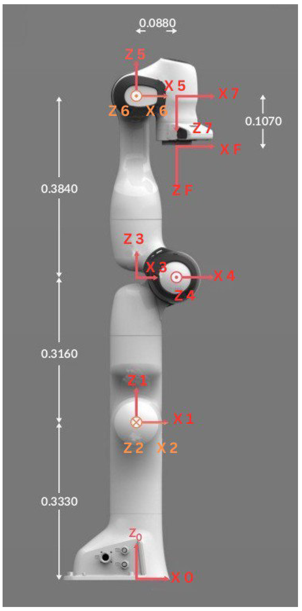
2. Modeling of Robotic Arm

Direct Kinematic Model of Robotic Arm

The rotation matrices in the Denavit–Hartenberg (DH) coordinate frame represent the rotations on the X and Z axes. The rotation matrices for these axes are respectively provided as follows:
R x = 1 0 0 0 C δ i S δ i 0 S δ i C δ i
and
R z = C ϕ i S ϕ i 0 S ϕ i C ϕ i 0 0 0 1 .
The homogeneous transformation matrix ( T i 1 i ) that accounts for rotation and translation is provided as follows:
T i 1 i = R i 1 i p i 1 i 0 1 = Rot x ( ϕ i ) · trans x ( d i ) · trans z ( Δ i ) · Rot z ( a i )
T i 1 i = C ϕ i S ϕ i C δ i S ϕ i S δ i a i C ϕ i S ϕ i C ϕ i C δ i C ϕ i S δ i a i S ϕ i 0 S δ i C δ i d i 0 0 0 1
where:
  • The rotation matrix ( R i 1 i ) represents the orientation of the i-th frame relative to the ( i 1 ) -th frame.
  • P i 1 i represents the center of the link frame with components ( P x , P y , and P z ).

Denavit–Hartenberg (DH) Axis Representation

The four DH parameters that describe the translation and rotation relationship between two consecutive coordinate frames are as follows:
  • d: Distance between the current frame and the previous frame along the Z-axis,
  • ( ϕ ): Angle between the X-axis of the previous frame and the X-axis of the current frame about the previous z-axis,
  • a: Distance between the Z-axes of the current and previous frames.
  • δ : offset of the previous frame from the current frame along the Z-axis of the current frame.
The Denavit–Hartenberg (DH) parameters for the Franka Panda robot shown in Figure 1 are provided in Table 1. From the above DH parameters and based on the homogeneous transformation matrix (3), the transformation matrix for the Franka Panda robot is derived as shown below.
T i 1 i = C ϕ i S ϕ i C δ i S ϕ i S δ i a i C ϕ i S ϕ i C ϕ i C δ i C ϕ i S δ i a i S ϕ i 0 S δ i C δ i d i 0 0 0 1
T 0 1 = C ϕ 1 S ϕ 1 0 0 S ϕ 1 C ϕ 1 0 0 0 0 1 0.33 0 0 0 1
T 1 2 = C ϕ 2 0 S ϕ 2 0 S ϕ 2 0 C ϕ 2 0 0 1 0 0 0 0 0 1
T 2 3 = C ϕ 3 0 S ϕ 3 0 S ϕ 3 0 C ϕ 3 0 0 1 1 0.316 0 0 0 1
T 3 4 = C ϕ 4 0 S ϕ 4 0.0825 C ϕ 4 S ϕ 4 0 C ϕ 4 0.0825 S ϕ 4 0 1 1 0 0 0 0 1
T 4 5 = C ϕ 5 0 S ϕ 5 0.0825 C ϕ 5 S ϕ 5 0 C ϕ 5 0.0825 S ϕ 5 0 1 0 0.384 0 0 0 1
T 5 6 = C ϕ 6 0 S ϕ 6 0 S ϕ 6 0 S ϕ 6 0 0 1 0 0 0 0 0 1
T 6 7 = C ϕ 7 0 S ϕ 7 0.088 C ϕ 7 S ϕ 7 0 C ϕ 7 0.088 S ϕ 7 0 1 0 0 0 0 0 1
T 7 0 = T 0 1 · T 1 2 · T 2 3 · T 3 4 · T 4 5 · T 5 6 · T 6 7
T 7 0 = r 11 r 12 r 13 p x r 21 r 22 r 23 p y r 31 r 32 r 33 p z 0 0 0 1
The orientation and position of the end effector are respectively provided by
R 11 = S ϕ 1 S ϕ 3 C ϕ 2 + C ϕ 1 C ϕ 3 C ϕ 4
R 12 = S ϕ 1 C ϕ 2 C ϕ 3 C ϕ 4 S ϕ 3 C ϕ 1
R 13 = S ϕ 2 C ϕ 1
R 21 = S ϕ 1 C ϕ 3 C ϕ 4 + S ϕ 3 C ϕ 1 C ϕ 2
R 22 = S ϕ 1 S ϕ 3 C ϕ 2 + C ϕ 1 C ϕ 3 C ϕ 4
R 23 = S ϕ 2 S ϕ 1
R 31 = S ϕ 2 C ϕ 3 C ϕ 4
R 32 = S ϕ 2 S ϕ 3 C ϕ 4
R 33 = C ϕ 2
and
p x = 0.107 S ϕ 2 C ϕ 1 + 0.088 C ϕ 1 + 0.384 S ϕ 1 S ϕ 3 C ϕ 2 + C ϕ 1 C ϕ 3 C ϕ 4 + 0.316 C ϕ 1 C ϕ 2 + 0.333 C ϕ 1
p y = 0.107 S ϕ 2 S ϕ 1 + 0.088 S ϕ 1 + 0.384 S ϕ 1 C ϕ 3 C ϕ 4 + S ϕ 3 C ϕ 1 C ϕ 2 + 0.316 S ϕ 1 C ϕ 2 + 0.333 S ϕ 1
p z = 0.107 C ϕ 2 + 0.384 S ϕ 2 C ϕ 3 C ϕ 4 + 0.316 S ϕ 2 + 0.333 S ϕ 2 .

3. Deep Reinforcement Learning Algorithm Design

3.1. Policy Gradient Algorithm

The policy gradient theorem states that the expected return to the policy parameters can be calculated as the sum of the action value function q π ( s , a ) multiplied by the policy function π ϱ ( s , a ) , summed over all states s and actions a and weighted by the stationary distribution of states d π ( s ) :
O ( ϱ ) = s d π ( s ) a Q π ( s , a ) π ϱ ( s , a )
where:
  • Objective function ( J ϱ ): This represents the expected cumulative reward obtained by following the policy π ϱ in the given environment. The objective function is optimized by adjusting the parameter ϱ to maximize the expected cumulative reward.
  • Discounted state distribution ( d π ( s ) ): This represents the probability of being in a particular state s under the policy π ; mathematically,
    d π ( s ) = lim t P ( s t = s | s 0 , π ϱ ) ,
    where s t = s when starting from s 0 and following policy π ϱ for t time steps.
  • Action–value function ( Q π ( s , a ) ): This represents the expected cumulative reward obtained by taking action a in state s and following policy π thereafter.
  • Policy function( π ϱ ( s , a ) ): This represents the probability of taking action a in state s under the parameterized policy ϱ .
The policy gradient theorem helps to solve this problem by providing a formula for the gradient of the expected return to the policy parameters. This formula involves the stationary distribution of the Markov chain, and is provided by
ϱ J ϱ = s d π ( s ) a q π ( s , a ) ϱ π ϱ ( a | s ) ,
where q π ( s , a ) is the state–action value function for policy π ϱ :
s S d π ( s ) a A Q π ( s , a ) ϱ π ϱ ( s , a ) .

3.1.1. Derivation of the Policy Gradient Theorem

The steps of the derivation using the derivative product rule of Equation (29) are as follows:
ϱ V π ( s ) = ϱ a A π ϱ ( a | s ) Q π ( s , a ) ,
using the derivative product rule
= a A ( ϱ π ϱ ( a | s ) Q π ( s , a ) + π ϱ ( a | s ) ϱ Q π ( s , a ) ) .
Step 1: Apply the derivative product rule:
ϱ V π ( s ) = ϱ a A ( π ϱ ( a | s ) Q π ( s , a ) ) .
Step 2: Distribute the derivative operator inside the summation:
ϱ V π ( s ) = a A ϱ ( π ϱ ( a | s ) Q π ( s , a ) ) .
Step 3: Apply the chain rule to differentiate the product of π ϱ ( a | s ) and Q π ( s , a ) from ϱ :
ϱ V π ( s ) = a A ϱ π ϱ ( a | s ) Q π ( s , a ) + π ϱ ( a | s ) ϱ Q π ( s , a ) .
Step 4: Simplify the expression by rearranging the terms.
After applying the derivative product rule, the derivative of the state–value function V π ( s ) to the policy parameter ϱ is
ϱ V π ( s ) = a A ϱ π ϱ ( a | s ) Q π ( s , a ) + π ϱ ( a | s ) ϱ Q π ( s , a ) .
We can extend Q π ( s , a ) by incorporating the value of the future state. This can be done by considering the state–action pair ( s , a ) and summing over all possible future states s and corresponding rewards r:
= a A [ ϱ π ϱ ( a | s ) Q π ( s , a ) + π ϱ ( a | s ) ϱ s , r P ( s , r | s , a ) ( r + V π ( s ) ) ] .
Because P ( s , r | s , a ) and r are not functions of ϱ , the derivative operator ϱ can be moved inside the summation over s , r without affecting these terms:
ϱ V π ( s ) = a A [ ϱ π ϱ ( a | s ) Q π ( s , a ) + π ϱ ( a | s ) s , r P ( s , r | s , a ) ϱ V π ( s ) ] .
Next, we can observe that ϱ V π ( s ) is the derivative of the state–value function from the policy parameter ϱ at state s . This can be rewritten as ϱ V π ( s ) = ϱ V π ( s ) s P ( s | s , a ) . Here, P ( s | s , a ) represents the probability of transitioning to state s given the current state–action pair ( s , a ) . We can now make the following substitution:
= a A ϱ π ϱ ( a | s ) Q π ( s , a ) + π ϱ ( a | s ) s , r P ( s , r | s , a ) ϱ V π ( s )
= a A ϱ π ϱ ( a | s ) Q π ( s , a ) + π ϱ ( a | s ) s P ( s | s , a ) ϱ V π ( s )
where P ( s | s , a ) = r P ( s | s , a ) .
Now, we have
ϱ V π ( s ) = a A [ ϱ π ϱ ( a | s ) Q π ( s , a ) + π ϱ ( a | s ) s P ( s | s , a ) ϱ V π ( s ) ] .
We can consider the following visit sequence and identify the probability of changing state s to state x using policy π ϱ after k steps as ρ ( s x , k ) :
s a π ϱ ( . | s ) s a π ϱ ( . | s ) s a π ϱ ( . | s )
  • For k = 0 : ρ ( s s , k = 0 ) = 1 , and
  • For k = 1 , we can consider every action that might be taken and add up the probabilities of reaching the desired state:
    ρ ( s x , k = 1 ) = a π ϱ ( a | s ) P ( s | s , a ) .
  • The goal is to move from s to x after k + 1 steps by following π ϱ . The agent can first move from s to intermediate state s ( s S ) before proceeding to the final state x in the last steps after k stages. This allows us to recursively update the visitation probability as
    ρ ( s x , k + 1 ) = s ρ π ( s s , k ) ρ ( s x , 1 ) .
After dealing with the probability ρ ( s x , k ) for transitioning from state s to state x after a certain number of steps k, the next step is to drive a recursive formulation for ϱ V π ( s ) .
To accomplish this, a function ϕ ( s ) is introduced and defined as follows:
ϕ ( s ) = a A ϱ π ϱ ( a | s ) Q π ( s , a )
where Φ ( s ) represents the sum of the gradients of the policy π ϱ to ϱ , weighted by the corresponding action–value function Q π ( s , a ) .
To simplify,
ϱ V π ( s ) = Φ ( s ) + a A π ϱ ( a | s ) s P ( s | s , a ) ϱ V π ( s )
= ϕ ( s ) + a π ϱ ( a | s ) s P ( s | s , a ) ϱ V π ( s )
= Φ ( s ) + s a A π ϱ ( a | s ) P ( s | s , a ) ϱ V π ( s )
= Φ ( s ) + s ρ π ( s s , 1 ) ϱ V π ( s )
= Φ ( s ) + s ρ π ( s s , 1 ) ϕ ( s ) + s ρ π ( s s , 1 ) ϱ V π ( s ) .
Considering s as the middle point for s s ,
= Φ ( s ) + s ρ π ( s s , 1 ) ϕ ( s ) + s ρ π ( s s , 2 ) ϱ V π ( s ) .
The expression for ϱ V π ( s ) can be unrolled as follows:
= Φ ( s ) + s ρ π ( s s , 1 ) Φ ( s ) + s ρ π ( s s , 2 ) Φ ( s ) + s ρ π ( s s , 3 ) ϱ V π ( s )
ϱ V π ( s ) = x S k = 0 ρ π ( s x , k ) Φ ( x ) .
Eliminating the derivatives of the Q-value function ϱ Q π ( s ) and inserting objective function O ( ϱ ) , starting from state S 0 ,
ϱ O ( ϱ ) = ϱ V π ( S 0 ) ,
= s k = 0 ρ π ( s x , k ) ϕ ( s ) .
Letting η ( s ) = s ρ π ( s , x , k ) ,
ϱ O ( ϱ ) = s η ( s ) ϕ ( s ) .
Substituting η ( s ) = s ρ π ( s , x , k ) into Equation (47),
ϱ O ( ϱ ) = s η ( s ) ϕ ( s ) .
We can normalize η ( s ) , s S to be the probability distribution, as shown in
ϱ O ( ϱ ) = s η ( s ) s η ( s ) s η ( s ) ϕ ( s ) .
Because s η ( s ) is constant, the gradient of the objective function is proportional to the normalized η ( s ) and ϕ ( s ) :
ϱ O ( ϱ ) s η ( s ) s η ( s ) ϕ ( s )
where d π ( s ) = η ( s ) s η ( s ) is a stationary distribution.
In the episodic case, the constant proportionality s η ( s ) is the average length of an episode, while in the continuing case it is 1 [36]:
= s d π ( s ) a A ϱ π ϱ ( a | s ) Q π ( s , a )
ϱ O ( ϱ ) s S d π ( s ) a A Q π ( s , a ) ϱ π ( ϱ ) ( a | s )
ϱ O ( ϱ ) = s S d π ( s ) ϱ π ( ϱ ) ( a | s ) π ( ϱ ) ( a | s )
= s S d π ( s ) ϱ π ( ϱ ) ( a | s ) π ( ϱ ) ( a | s )
ϱ O ( ϱ ) = E π { Q π ( s , a ) ϱ ln ( π ϱ ( a | s ) ) }
where E π refers to E s d π , a π ϱ when the distribution of the states and actions follows policy π ϱ (on-policy).

3.1.2. Off-Policy Gradient Algorithms

Because DDPG is an off-policy gradient algorithm, we first discuss this type of policy gradient algorithm in more detail.
The behavior policy for collecting samples is known and labeled as α ( a | s ) . The objective function sums up the reward over the state distribution defined by this behavior policy:
O ( ϱ ) = s S d α ( s ) a A Q π ( s , a ) π ϱ ( a | s )
= E s d α a A Q π ( s , a ) π ϱ ( a | s )
where d α ( s ) is the stationary distribution of behavior policy α , as d α ( s ) = lim t P ( S t = s | S 0 , α ) and Q π is the action–value function estimated about the target policy π . Given that the training observations are sampled by a α ( a | s ) , we can rewrite the gradient as
ϱ O ( ϱ ) = ϱ E s d α a A Q π ( s , a ) π ϱ ( a | s )
by using the derivative product rule
= E s d α a A Q π ( s , a ) ϱ π ϱ ( a | s ) + π ϱ ( a | s ) ϱ Q π ( s , a )
and ignoring π ϱ ( a | s ) ϱ Q π ( s , a ) :
( i ) E s d α a A Q π ( s , a ) ϱ π ϱ ( a | s )
= E s d α a A α ( a | s ) π ϱ ( a | s ) α ( a | s ) Q π ( s , a ) ϱ π ϱ ( a | s ) π ϱ ( a | s )
= E α π ϱ ( a | s ) α ( a | s ) Q π ( s , a ) ϱ ln π ϱ ( a | s )
where π ϱ ( a s ) α ( a s ) is the importance weight. Because Q π is a function of the target policy, and consequently a function of the policy parameter ϱ , the derivative ϱ Q π ( s , a ) must also be computed using the product rule. However, in practice it is challenging to compute ϱ Q π ( s , a ) directly. Fortunately, policy improvement can still be guaranteed by approximating the gradient and ignoring the gradient of Q π , which achieves eventual convergence to the true local minimum.
In summary, when applying the policy gradient in the off-policy setting, it can be adjusted using a weighted sum, where the weight is the ratio of the target policy to the behavior policy, π ϱ ( a | s ) α ( a | s ) [36].

3.2. Deterministic Policy Gradient (DPG)

The policy function π ( · | s ) is typically represented as a probability distribution over actions (A) based on the current state, making it inherently stochastic. However, in the case of the DPG, the policy is modeled as a deterministic decision, denoted as a = μ ( s ) . Instead of selecting actions probabilistically, the DPG directly maps states to specific actions without uncertainty. Let
  • ρ 0 ( s ) be the initial distribution over states,
  • ρ μ ( s s , k ) be the density of visitation probability in state s when starting from state s after moving k steps by policy μ , and
  • ρ μ ( s ) be the discounted state distribution, defined as
    ρ μ ( s ) = S k = 1 γ k 1 ρ 0 ( s ) ρ μ ( s s , k ) d s .
Then, the objective function to be optimized is
O ( ϱ ) = S ρ μ ( s ) Q ( s , μ ϱ ( s ) ) d s .
According to the chain rule, we first take the gradient of Q with respect to action a, then take the gradient of the deterministic policy function μ with respect to ϱ :
ϱ O ( ϱ ) = S ρ μ ( s ) a Q μ ( s , a ) ϱ μ ϱ ( s ) | a = μ ϱ ( s ) d s ,
= E s ρ μ [ a Q μ ( s , a ) ϱ μ ϱ ( s ) | a = μ ϱ ( s ) ] .

3.3. Deep Deterministic Policy Gradient (DDPG)

By combining DQN and DPG, DDPG leverages the power of deep neural networks to handle high-dimensional state spaces and complex action spaces, making it suitable for a wide range of reinforcement learning tasks. The original DQN works in discrete space; DDPG extends it to continuous space with the actor–critic framework while learning a deterministic policy. To improve exploration, an exploration policy μ is constructed by adding noise N :
μ ( s ) = μ ϱ ( s ) + N .
Moreover, the DDPG algorithm integrates a sophisticated technique known as soft updates, also called conservative policy iteration, to update the parameters of both the actor and critic networks. This revised methodology utilizes a small parameter, denoted τ , which is much smaller than 1 ( τ 1 ).
The soft update equation is formulated as follows:
ϱ τ ϱ + ( 1 τ ) ϱ .
Unlike the approach employed in the DQN, this guarantees that the target network values are gradually altered over time when the target network remains static for a fixed period.
As shown in Algorithm 1, the DDPG algorithm follows an actor-critic framework where the critic network estimates the action-value function, while the actor network learns a deterministic policy. The training process begins with initializing the networks and reply buffer. During each episode, actions are selected using the current policy with added exploration noise, and the resulting transition is stored in the reply buffer. The critic is updated by minimizing the loss function, and the actor is optimized using the policy gradient. Furthermore, the target networks for both the actor and the critic are updated using soft updates to ensure stability in learning [37].
Algorithm 1: Deep Deterministic Policy Gradient [37]
Actuators 14 00165 i001

4. Results and Discussion

4.1. Simulation Environment and Training Setup

The deep reinforcement learning agent was trained using Python on a Jupyter Notebook using a Linux Ubuntu 20.04 operating system. The training process spanned approximately 5.415 h on a system with an Intel graphics card, 8 GB of RAM, and a 1.9 GHz processor.
To simulate the target reaching task of the Franka Panda robotic arm, we utilized the PandaReach-v2 environment from the panda_gym library, which is built on PyBullet. This physics-based environment enables realistic interactions for reinforcement learning.
To train the Deep Deterministic Policy Gradient (DDPG) algorithm, Stable Baselines3, an optimized deep-reinforcement learning library was used. The training process spanned 100,000 time steps, allowing the robotic agent to learn an optimal policy for precise target reaching. The integration of OpenAI Gym, PyBullet, and Panda Gym provided an efficient and flexible simulation framework to evaluate reinforcement learning techniques in robotic manipulation.

4.2. Hyperparameter Selection and Initial Search

The parameters listed in Table 2 were selected for this work.

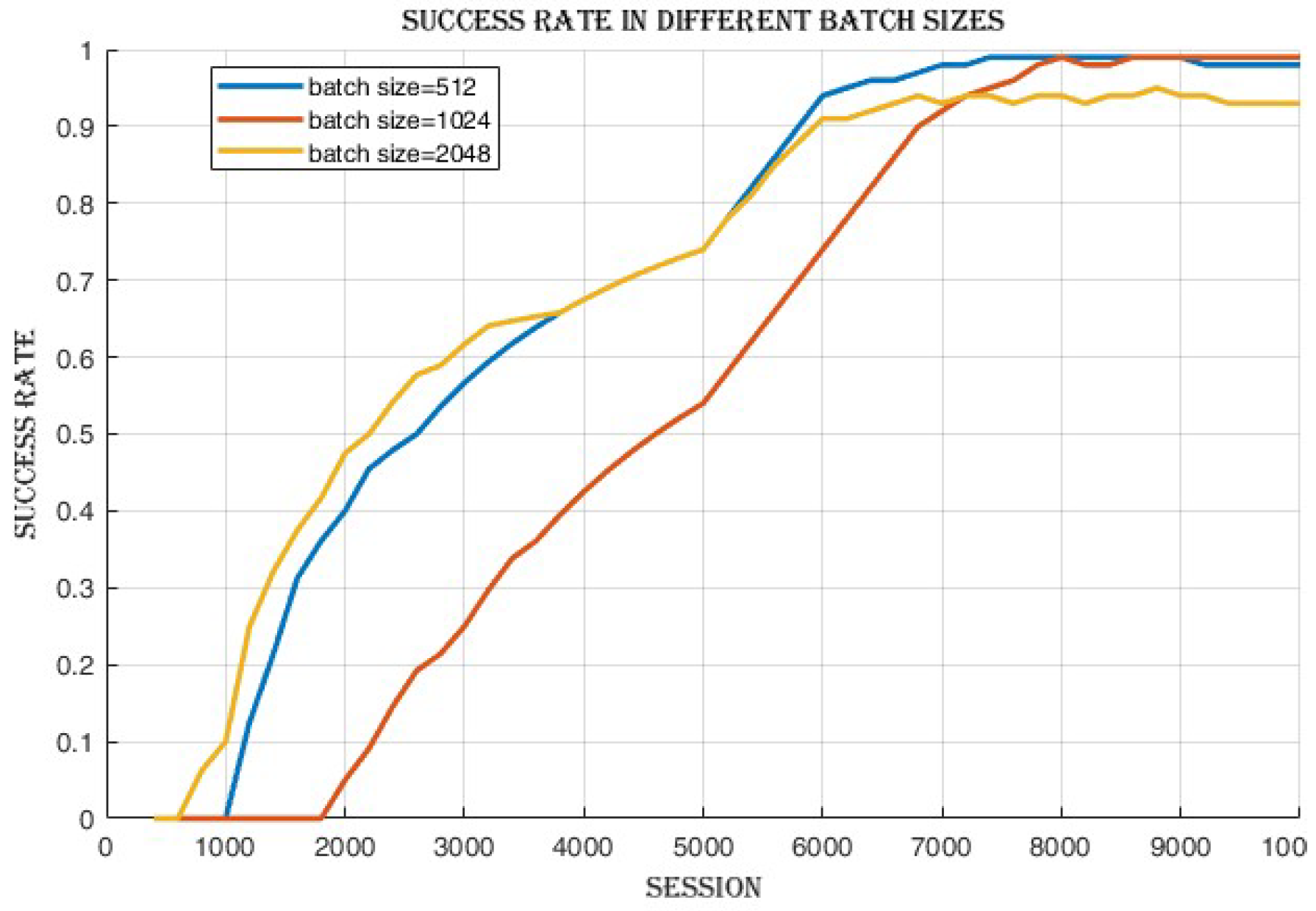
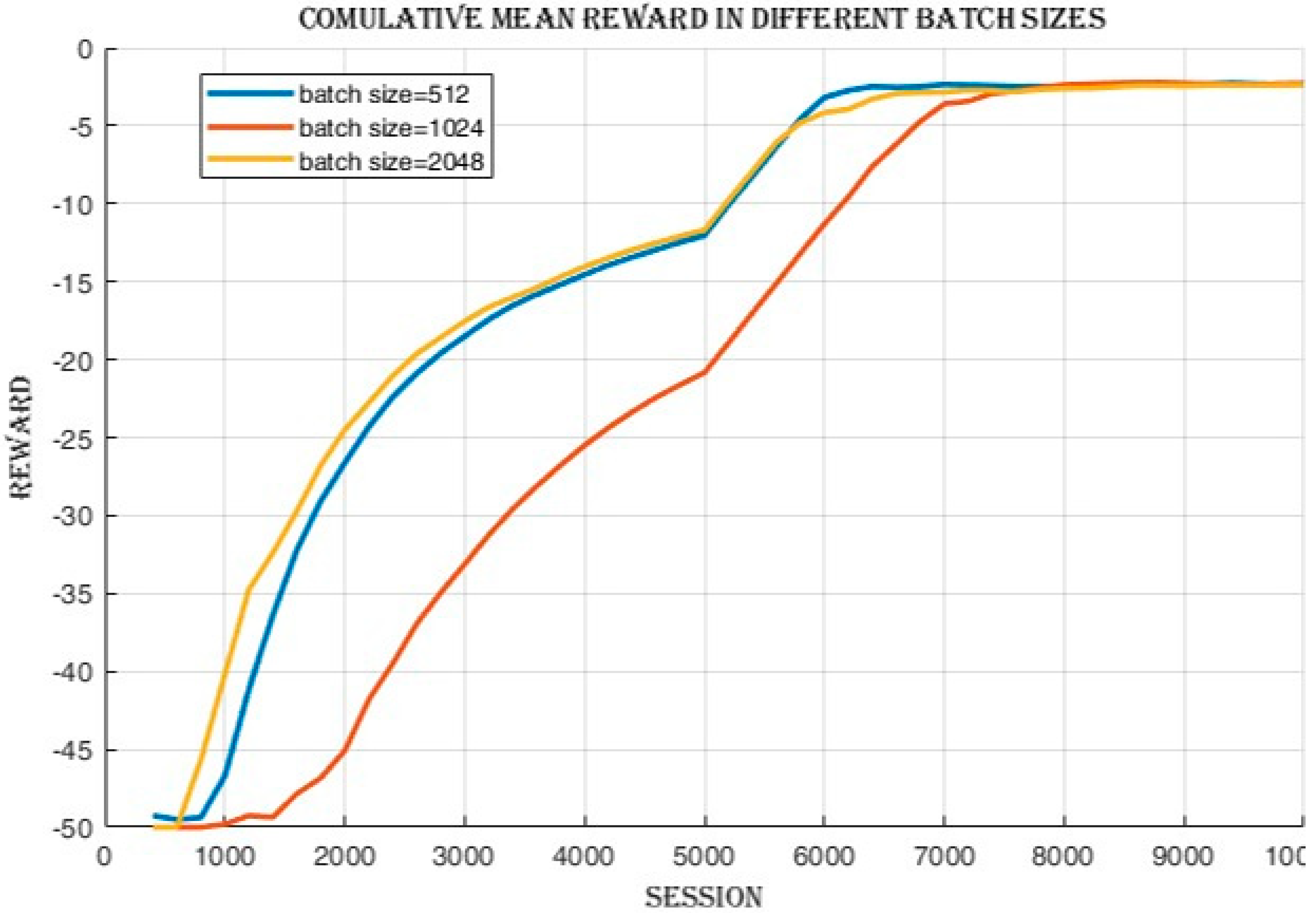
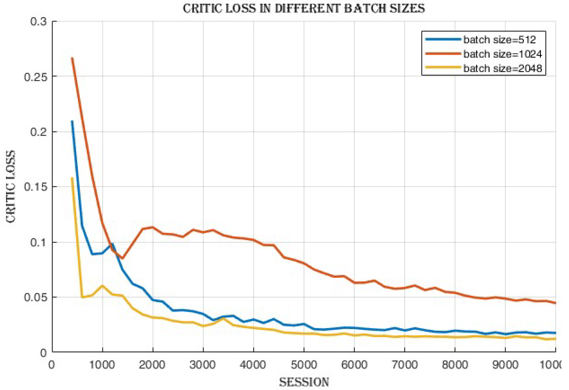
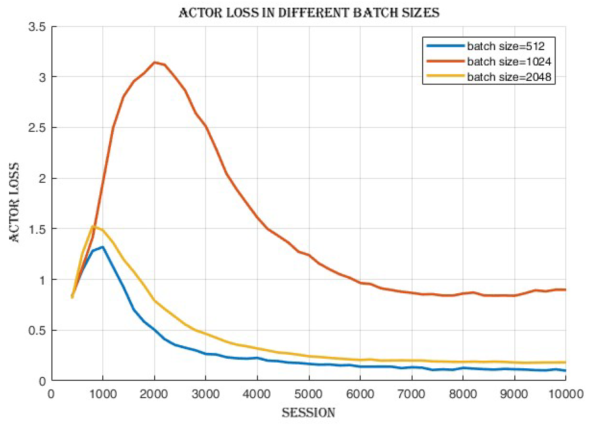
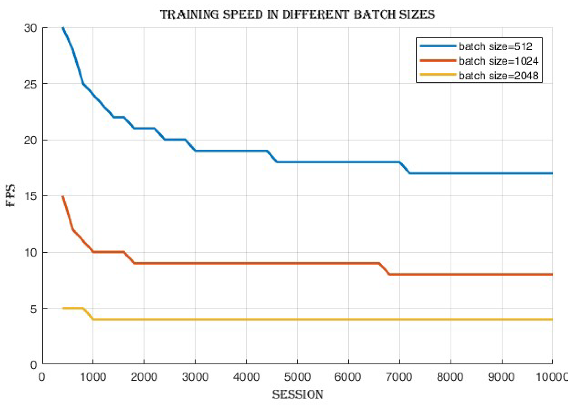
4.2.1. Batch Size Comparison

Upon completion of the training process, it was observed that there was a minimal disparity in the success rate (Figure 2) and the cumulative reward (Figure 3) between the different batch sizes. Furthermore, the decrease in critic loss values (Figure 4) and actor loss values (Figure 5) indicated an improvement in the ability of both the actor and critic networks to approximate the optimal policy and value functions. Although the success rate and cumulative reward were similar, the enhanced convergence demonstrated by the lower losses with a batch size of 2048 suggests a more efficient learning process and a potentially higher quality of the policies learned within this setting. However, as Figure 6 shows, the training speed varied widely with batch sizes, with 512 being the fastest, 1024 second, and 2048 last. Despite its slower training speed, a batch size of 2048 was used because it achieved better stability and convergence. Larger batch sizes generally reduce gradient variance, leading to a smoother optimization process and improved overall model quality.

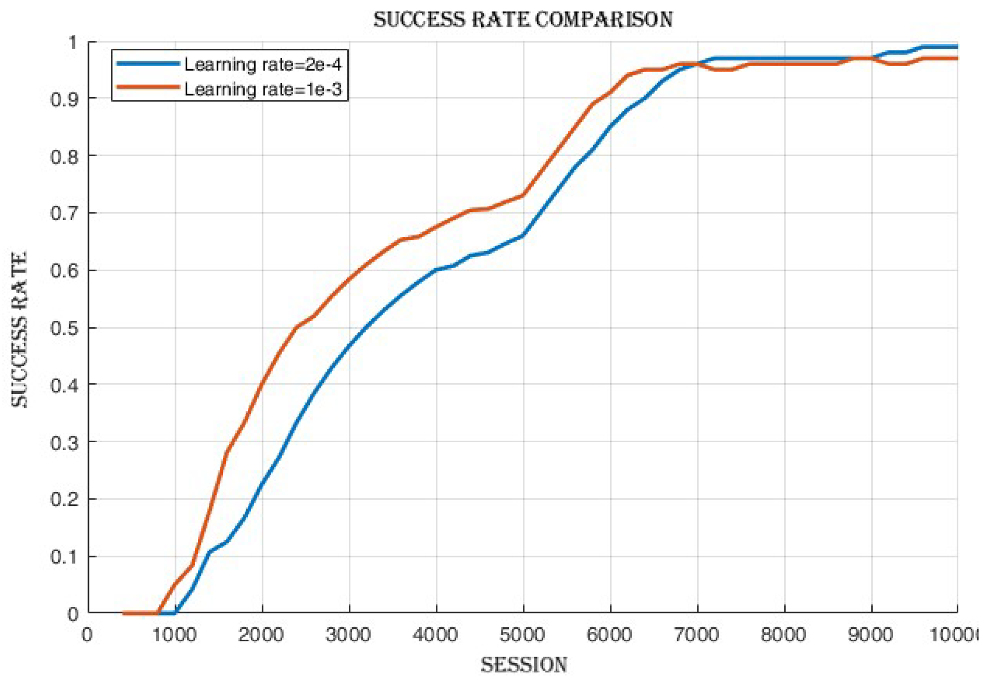
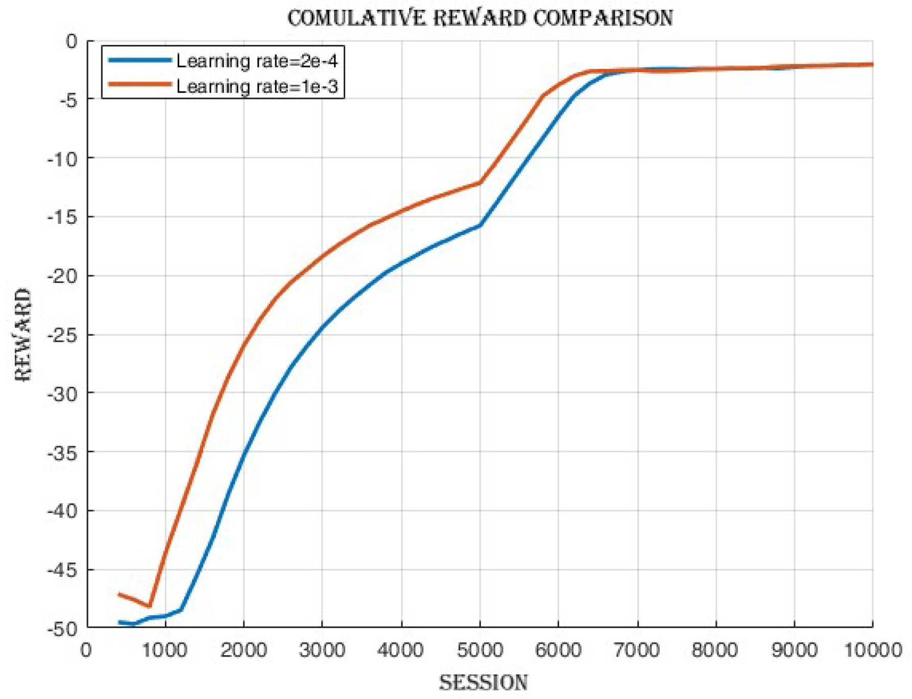
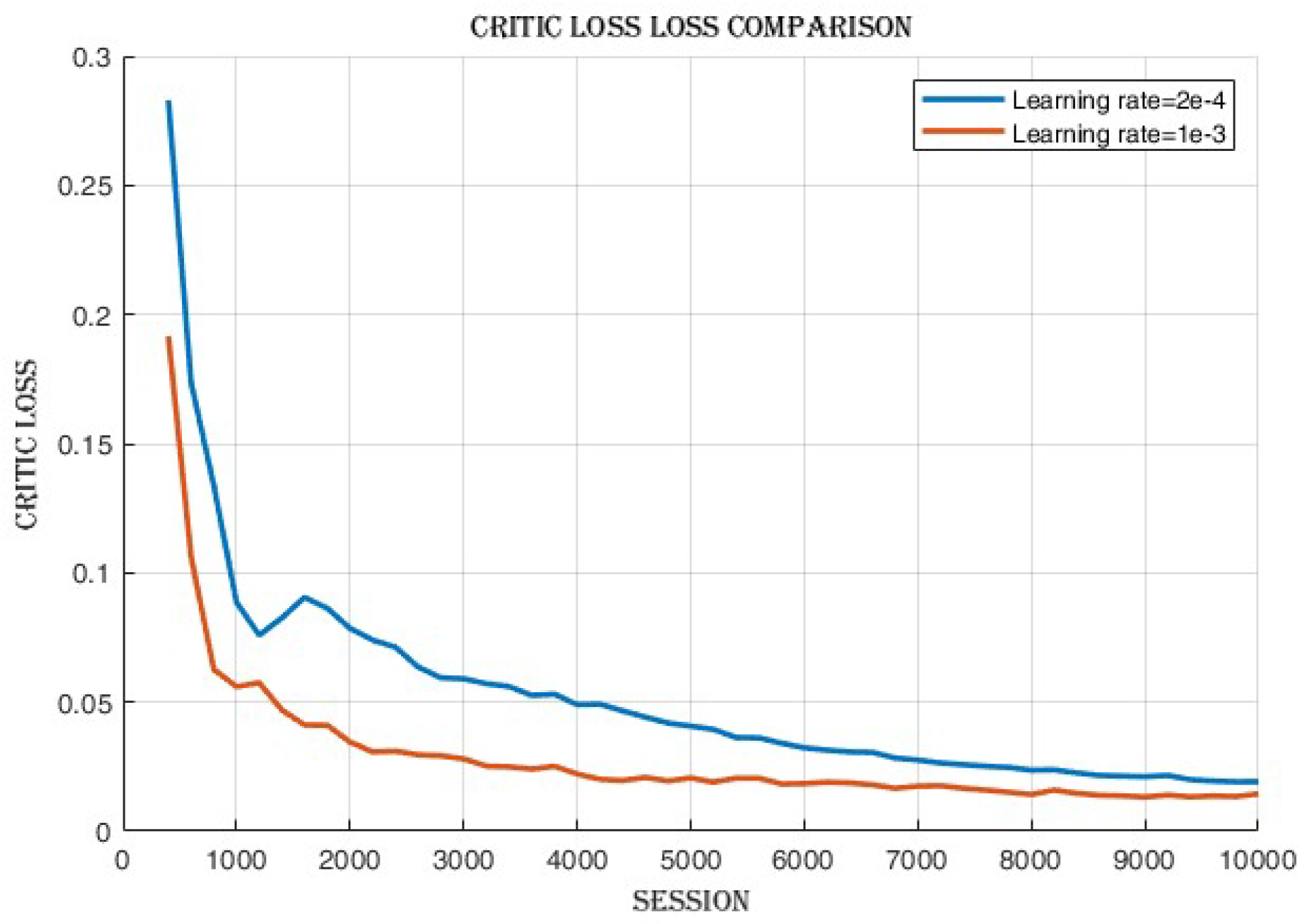
4.2.2. Learning Rate Comparison

After the training process, the observations shown in Figure 7 and Figure 8 revealed a minimal disparity in the cumulative reward and the success rate achieved between the two learning rates. However, the learning rate of 2e-4 shows a slightly better success rate compared to the learning rate of 1e-3. In contrast, when using the learning rate of 1e-3, a notable decrease in both actor loss (Figure 9) and critic loss (Figure 10) was observed, indicating improved policy and value estimation. Despite comparable cumulative reward and success rates, the reduced losses with the learning rate of 1e-3 signified enhanced convergence and a potentially more efficient learning process, suggesting that the agent may have acquired higher-quality learned policies.

4.3. Selection of Optimal Hyperparameters and Extended Training of DDPG Agent

After comparing the hyperparameters and performing a detailed analysis of the associated results, we selected the hyperparameters with the most promising performance as shown in Table 3. Following this, an extended training phase was initiated that included 100,000 time steps as shown in Table 4. This extended training phase served as the fundamental training stage, which is elaborated in the following section.

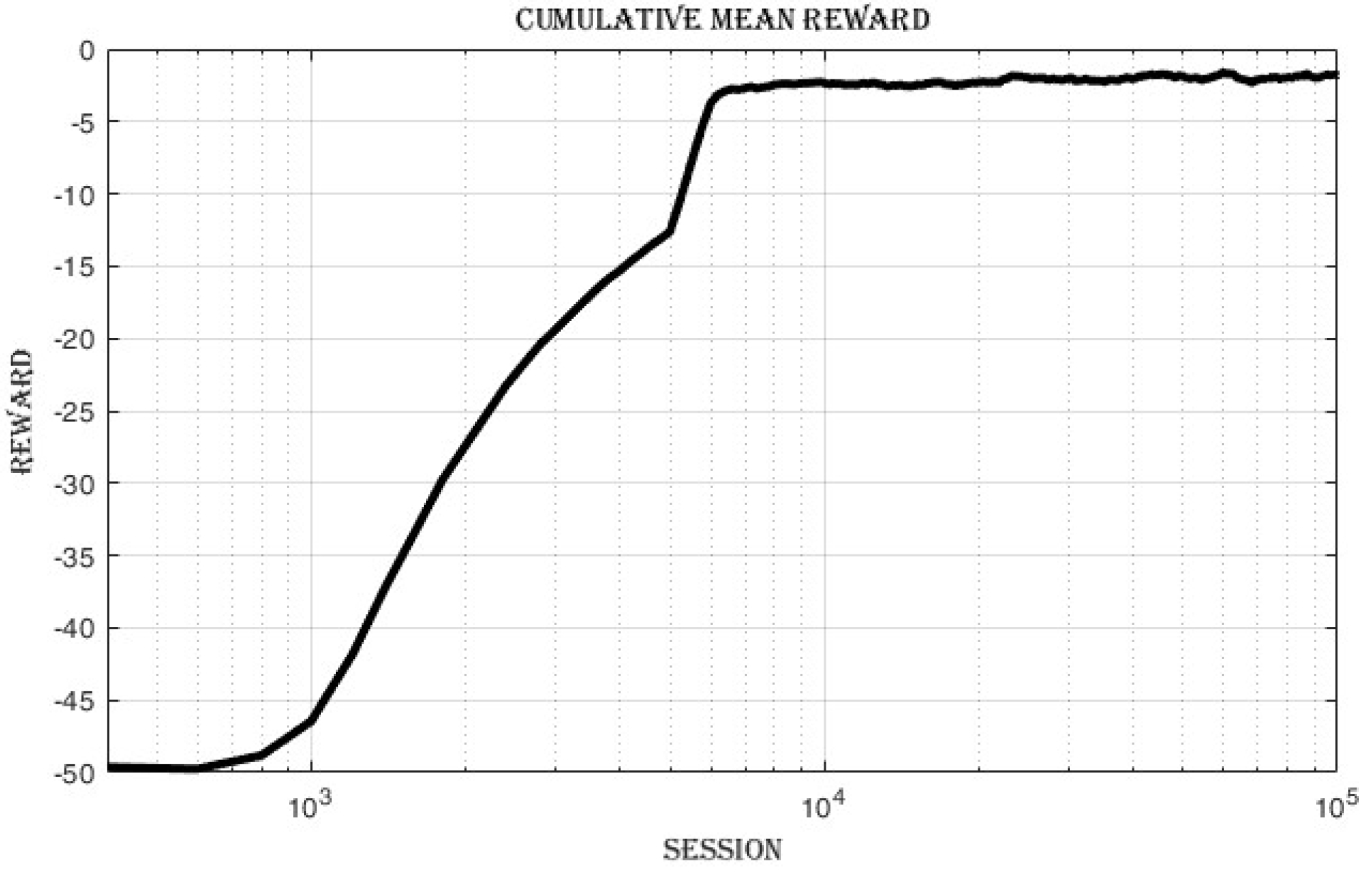
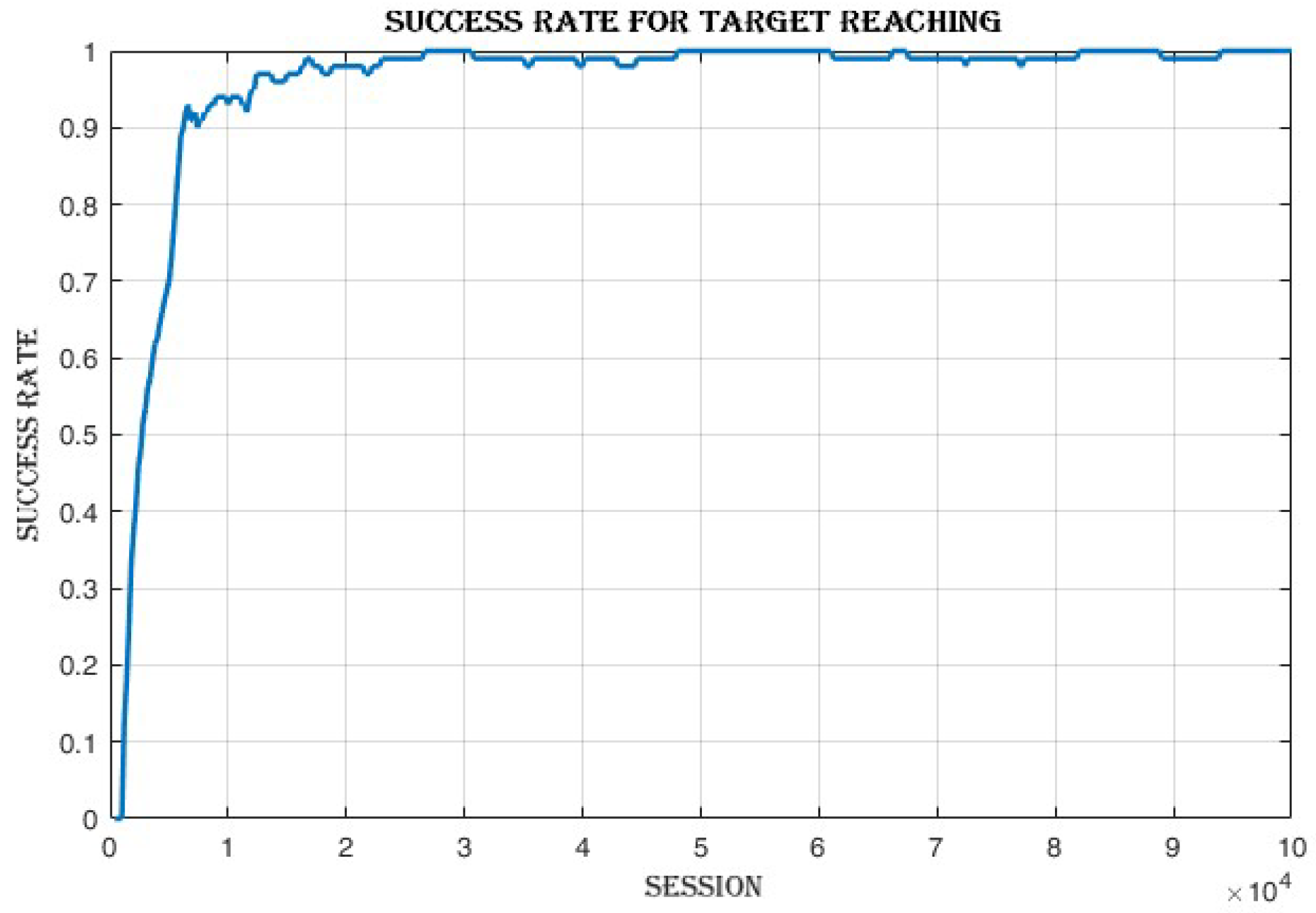
4.3.1. Improvement in Cumulative Reward and Success Rate

The mean episode reward (Figure 11) improved from −49.2 in the first loop to −1.8 in the last loop, while the success rate (Figure 12) increased from 0 in the first loop to 1 in the last loop.

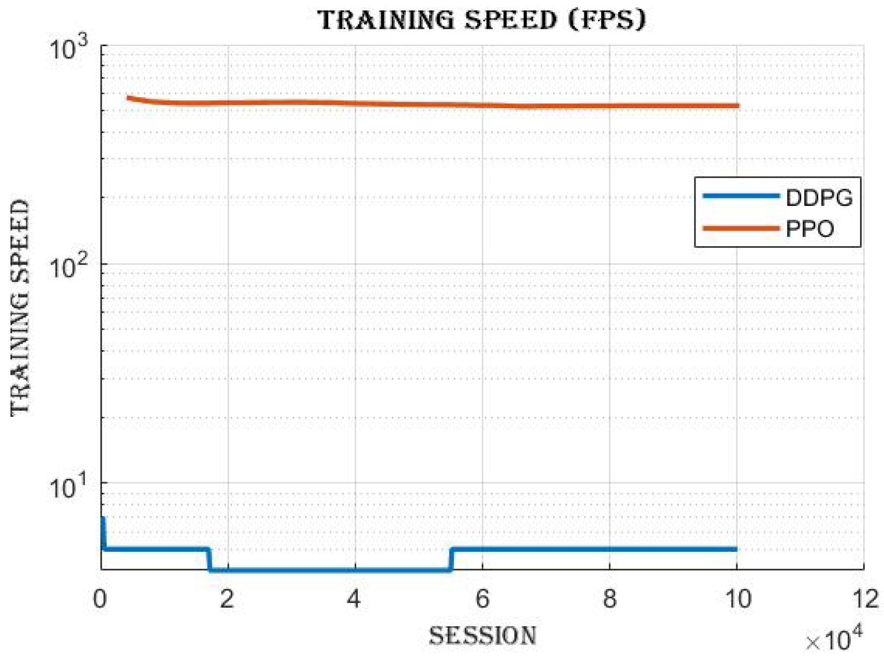
4.3.2. Frames per Second (FPS)

The training speed (Figure 13) decreased from 18 frames per second (FPS) in the first loop to 5 FPS in the last loop.

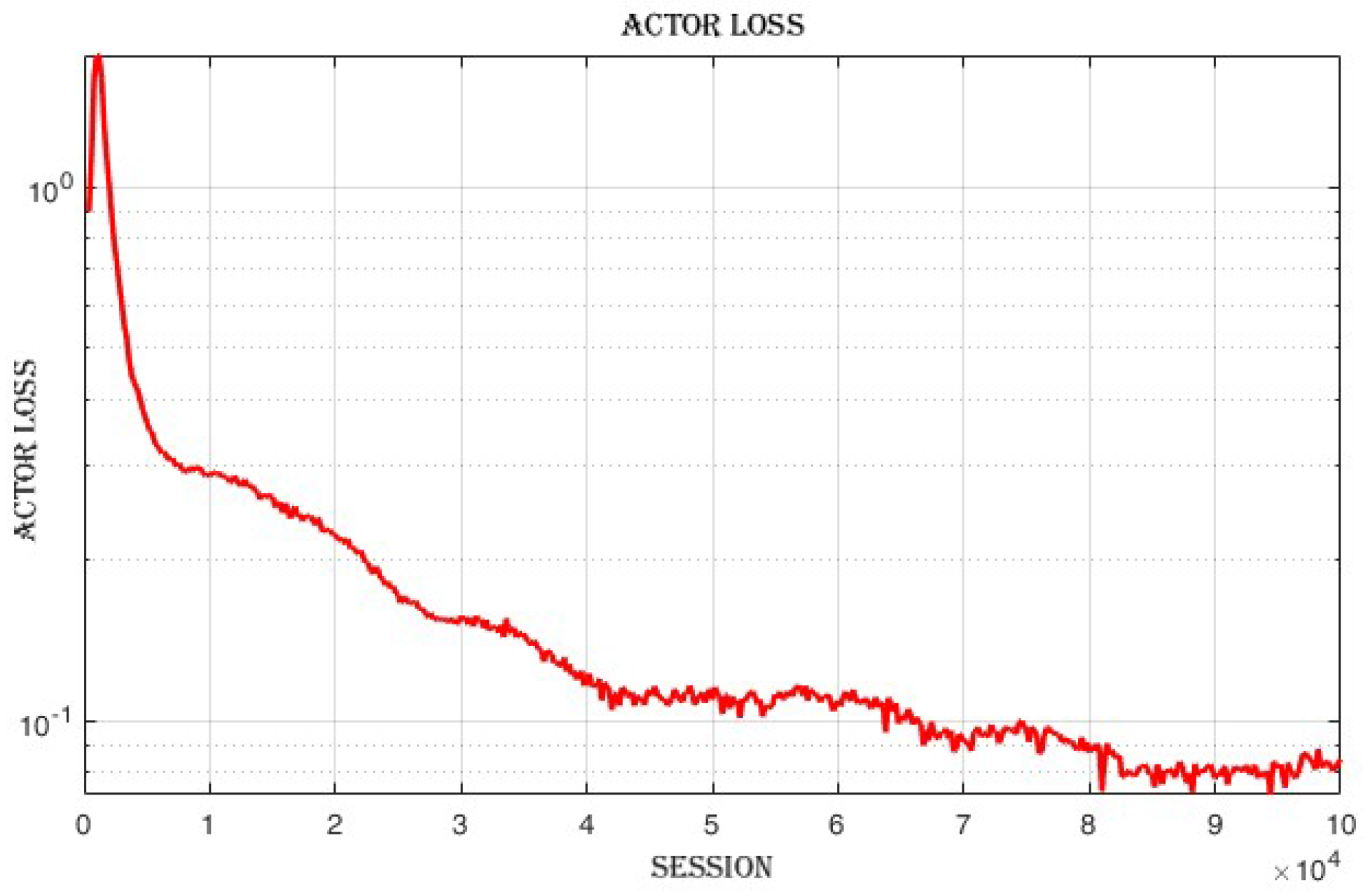
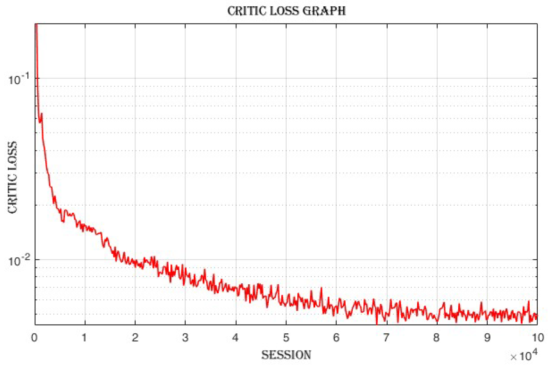
4.3.3. Improvement in Actor and Critic Losses

The actor loss (Figure 14) decreased from 0.625 in the first loop to 0.0846 in the last loop, while the critic loss (Figure 15) decreased from 0.401 in the first loop to 0.00486 in the last loop.

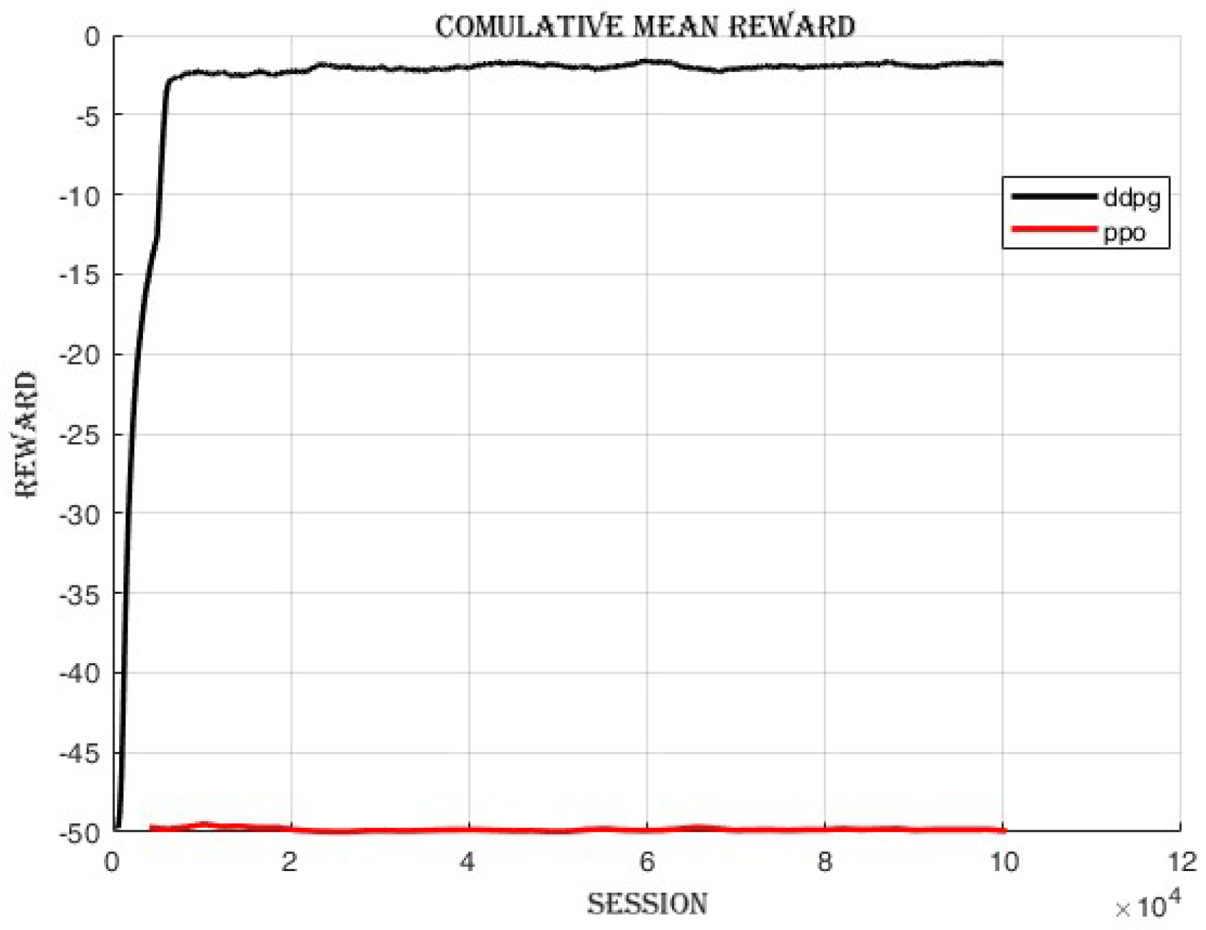
4.4. Comparing DDPG and PPO: Off-Policy vs. On-Policy Reinforcement Learning Algorithms

We trained the Proximal Policy Optimization (PPO) on-policy reinforcement learning algorithm and compared its performance with the Deep Deterministic Policy Gradient (DDPG) off-policy algorithm. The results are shown in Figure 16 and Figure 17. As shown in Figure 16, the cumulative reward achieved by DDPG was 1.8 , while the cumulative reward obtained by PPO was 50 . The results of this comparison indicate that DDPG shows better performance in this particular scenario than PPO in terms of cumulative reward.

5. Conclusions

In this study, we applied the Deep Deterministic Policy Gradient (DDPG) algorithm to train a robotic arm manipulator, specifically the Franka Panda robotic arm, for a target-reaching task. The objective of this task was to enable the robotic arm to accurately reach a designated target position. The DDPG algorithm was chosen because of its effectiveness in continuous control tasks and its ability to learn policies with high-dimensional action spaces. Using a combination of deep neural networks and an actor–critic architecture, the DDPG algorithm was able to approximate the optimal policy for the robotic arm. When comparing the performance of PPO and DDPG algorithms after training for 100,000 time steps, PPO achieved a mean episode reward of 50 indicating that the agent struggled to achieve positive rewards on average. Despite training at a relatively fast speed of 561 F P S , these results suggest that the PPO algorithm faced challenges in finding successful strategies for the given task.
However, the DDPG algorithm demonstrated superior performance, with a mean episode reward of 1.8 . It achieved a success rate of 1, indicating consistent success in achieving the desired outcomes. Despite a slower training speed of 5 F P S , the DDPG algorithm showcased the ability to learn and improve its policy effectively over time. Based on these results, DDPG outperformed PPO in terms of cumulative reward and success rate in the given scenario.
From the above results, it can be concluded that PPO performs worse than DDPG, mainly because of the way each algorithm learns. PPO is a policy-based method, which means that it learns only from its most recent interactions and ignores past experiences. Although this promotes stability, it makes learning less effective because the agent constantly needs new data to improve. However, DDPG is an off-policy algorithm, meaning that it stores past experiences in a replay buffer and continues to learn them. This makes training more sample-efficient, which is especially useful for complex tasks such as robotic arm control.
Another key difference is how the two algorithms update their policies. PPO uses a clipping mechanism to prevent large policy changes, which helps with stability but can slow down learning, especially in high-dimensional action spaces. Meanwhile, DDPG uses deterministic updates, allowing it to fine-tune actions more precisely.
Although DDPG had a much slower training speed, it ultimately learned better strategies, leading to a higher success rate and better rewards compared to PPO.

Author Contributions

The authors’ contributions in this manuscript are stated as follows: conceptualization, L.H. and Y.A.; methodology, L.H.; software, L.H.; validation, A.T. and S.J.; formal analysis, L.H.; investigation, A.T., S.J.; resources, L.H.; data curation, L.H.; writing—original draft preparation, L.H.; writing—review and editing, Y.A., A.T., and S.J.; visualization, A.T. and L.H.; supervision, Y.A. and S.J.; project administration, S.J.; funding acquisition, S.J. All authors have read and agreed to the published version of the manuscript.

Funding

This study was supported by a research fund from Chosun University, 2024 under Grant K208419006.

Institutional Review Board Statement

Not applicable.

Informed Consent Statement

Not applicable.

Data Availability Statement

All of the required data in this work are available from the authors and can be provided upon request.

Conflicts of Interest

The authors declare no conflicts of interest. The funders had no role in the design of the study, in the collection, analysis, or interpretation of data, in the writing of the manuscript, or in the decision to publish the results.

References

  1. Mohsen, S.; Behrooz, A.; Roza, D. Artificial intelligence, machine learning and deep learning in advanced robotics, a review. Cogn. Robot. 2023, 3, 54–70. [Google Scholar]
  2. Santos, A.A.; Schreurs, C.; da Silva, A.F.; Pereira, F.; Felgueiras, C.; Lopes, A.M.; Machado, J. Integration of Artificial Vision and Image Processing into a Pick and Place Collaborative Robotic System. J. Intell. Robot. Syst. 2024, 110, 159. [Google Scholar] [CrossRef]
  3. Xinle, Y.; Minghe, S.; Lingling, S. Adaptive and intelligent control of a dual-arm space robot for target manipulation during the post-capture phase. Aerosp. Sci. Technol. 2023, 142, 108688. [Google Scholar]
  4. Abayasiri, R.A.M.; Jayasekara, A.G.B.P.; Gopura, R.A.R.C.; Kazuo, K. Intelligent Object Manipulation for a Wheelchair-Mounted Robotic Arm. J. Robot. 2024, 2024, 1516737. [Google Scholar] [CrossRef]
  5. Yi, J.; Zhang, H.; Mao, J.; Chen, Y.; Zhong, H.; Wang, Y. Review on the COVID-19 pandemic prevention and control system based on AI. Eng. Appl. Artif. Intell. 2022, 114, 105184. [Google Scholar] [CrossRef] [PubMed]
  6. Tang, Q.; Liang, J.; Zhu, F. A comparative review on multi-modal sensors fusion based on deep learning. Signal Process. 2023, 213, 109165. [Google Scholar] [CrossRef]
  7. Doewes, R.I.; Purnama, S.K.; Nuryadin, I.; Kurdhi, N.A. Human AI: Social robot decision-making using emotional AI and neuroscience. In Emotional AI and Human-AI Interactions in Social Networking; Garg, M., Koundal, D., Eds.; Academic Press: Cambridge, MA, USA, 2024; pp. 255–286. [Google Scholar] [CrossRef]
  8. Martin, J.G.; Muros, F.J.; Maestre, J.M.; Camacho, E.F. Multi-robot task allocation clustering based on game theory. Robot. Auton. Syst. 2023, 161, 104314. [Google Scholar]
  9. Nguyen, M.N.T.; Ba, D.X. A neural flexible PID controller for task-space control of robotic manipulators. Front. Robot. AI 2023, 9, 975850. [Google Scholar]
  10. Laurenzi, A.; Antonucci, D.; Tsagarakis, N.G.; Muratore, L. The XBot2 real-time middleware for robotics. Robot. Auton. Syst. 2023, 163, 104379. [Google Scholar] [CrossRef]
  11. Zhang, L.; Jiang, M.; Farid, D.; Hossain, M.A. Intelligent Facial Emotion Recognition and Semantic-Based Topic Detection for a Humanoid Robot. Expert Syst. Appl. 2013, 40, 5160–5168. [Google Scholar]
  12. Floreano, D.; Wood, R.J. Science, Technology, and the Future of Small Autonomous Drones. Nature 2015, 521, 460–466. [Google Scholar] [CrossRef] [PubMed]
  13. Chen, T.D.; Kockelman, K.M.; Hanna, J.P. Operations of a Shared, Autonomous, Electric Vehicle Fleet: Implications of Vehicle & Charging Infrastructure Decisions. Transp. Res. Part Policy Pract. 2016, 94, 243–254. [Google Scholar]
  14. Chen, Z.; Jia, X.; Riedel, A.; Zhang, M. A Bio-Inspired Swimming Robot. In Proceedings of the 2014 IEEE International Conference on Robotics and Automation (ICRA), Hong Kong, China, 31 May–7 June 2014; p. 2564. [Google Scholar]
  15. Ohmura, Y.; Kuniyoshi, Y. Humanoid Robot Which Can Lift a 30kg Box by Whole Body Contact and Tactile Feedback. In Proceedings of the 2007 IEEE/RSJ International Conference on Intelligent Robots and Systems, San Diego, CA, USA, 29 October–2 November 2007; pp. 1136–1141. [Google Scholar]
  16. Kappassov, Z.; Corrales, J.-A.; Perdereau, V. Tactile Sensing in Dexterous Robot Hands. Robot. Auton. Syst. 2015, 74, 195–220. [Google Scholar] [CrossRef]
  17. Gomes, N.; Martins, F.; Lima, J.; Wörtche, H. Deep Reinforcement Learning Applied to a Robotic Pick-and-Place Application; Springer: Berlin/Heidelberg, Germany, 2021; pp. 251–265. [Google Scholar] [CrossRef]
  18. Aryslan, M.; Yevgeniy, L.; Troy, H.; Richard, P. A deep reinforcement-learning approach for inverse kinematics solution of a high degree of freedom robotic manipulator. Robotics 2022, 11, 44. [Google Scholar]
  19. Serhat, O.; Enver, T.; Erkan, Z. Adaptive Cartesian space control of robotic manipulators: A concurrent learning based approach. J. Frankl. Inst. 2024, 361, 106701. [Google Scholar]
  20. Ladosz, P.; Weng, L.; Kim, M.; Oh, H. Exploration in deep reinforcement learning: A survey. Inf. Fusion 2022, 85, 1–22. [Google Scholar] [CrossRef]
  21. AlMahamid, F.; Grolinger, K. Reinforcement learning algorithms: An overview and classification. In Proceedings of the 2021 IEEE Canadian Conference on Electrical and Computer Engineering (CCECE), Virtual, 12–17 September 2021; pp. 1–7. [Google Scholar]
  22. Thrun, S.; Littman, M.L. Reinforcement Learning: An Introduction. AI Mag. 2000, 21, 103. [Google Scholar]
  23. Smruti, A. Deep reinforcement learning for robotic manipulation-the state of the art. arXiv 2017, arXiv:1701.08878. Available online: https://api.semanticscholar.org/CorpusID:9103068 (accessed on 21 February 2024).
  24. Jens, K.; Bagnell, J.A.; Jan, P. Reinforcement learning in robotics: A survey. Int. J. Robot. Res. 2013, 32, 1238–1274. [Google Scholar]
  25. Tianci, G. Optimizing robotic arm control using deep Q-learning and artificial neural networks through demonstration-based methodologies: A case study of dynamic and static conditions. Robot. Auton. Syst. 2024, 181, 104771. [Google Scholar]
  26. Andrea, F.; Elisa, T.; Nicola, C.; Stefano, G. Robotic Arm Control and Task Training through Deep Reinforcement Learning. arXiv 2020, arXiv:2005.02632v1. [Google Scholar]
  27. Shianifar, J.; Schukat, M.; Mason, K. Optimizing Deep Reinforcement Learning for Adaptive Robotic Arm Control. arXiv 2024, arXiv:2407.02503v1. [Google Scholar]
  28. Roman, P.; Jakub, K.; Radomil, M.; Martin, J. Deep-Reinforcement-Learning-Based Motion Planning for a Wide Range of Robotic Structures. Computation 2024, 12, 116. [Google Scholar] [CrossRef]
  29. Wanqing, X.; Yuqian, L.; Weiliang, X.; Xun, X. Deep reinforcement learning based proactive dynamic obstacle avoidance for safe human-robot collaboration. Manuf. Lett. 2024, 41, 1246–1256. [Google Scholar]
  30. Chua, K.; Calandra, R.; McAllister, R.; Levine, S. Deep reinforcement learning in a handful of trials using probabilistic dynamics models. Adv. Neural Inf. Process. Syst. 2018, 31. [Google Scholar]
  31. Levine, S.; Pastor, P.; Krizhevsky, A.; Quillen, D. Learning hand-eye coordination for robotic grasping with deep learning and large-scale data collection. Int. J. Robot. Res. 2018, 37, 421–436. [Google Scholar]
  32. Kathirgamanathan, A.; Mangina, E.; Finn, D.P. Development of a Soft Actor Critic deep reinforcement learning approach for harnessing energy flexibility in a Large Office building. Energy AI 2021, 5, 100101. [Google Scholar] [CrossRef]
  33. Li, P.; Chen, D.; Wang, Y.; Zhang, L.; Zhao, S. Path planning of mobile robot based on improved TD3 algorithm in dynamic environment. Heliyon 2024, 10, e32167. [Google Scholar] [CrossRef]
  34. Salas-Pilco, S.; Xiao, K.; Hu, X. Correction: Salas-Pilco et al. Artificial Intelligence and Learning Analytics in Teacher Education: A Systematic Review. Educ. Sci. 2023, 13, 897. [Google Scholar] [CrossRef]
  35. Franka Emika Documentation. Control Parameters Documentation. 2024. Available online: https://frankaemika.github.io/docs/control_parameters.html (accessed on 21 February 2024).
  36. Weng, L. Policy Gradient Algorithms. Lil’Log. 2018. Available online: https://lilianweng.github.io/posts/2018-04-08-policy-gradient (accessed on 21 February 2024).
  37. Lillicrap, T.P.; Hunt, J.J.; Pritzel, A.; Heess, N.; Tassa, Y.; Silver, D. Continuous control with deep reinforcement learning. arXiv 2015, arXiv:1509.02971. [Google Scholar] [CrossRef]
Figure 1. Denavit –Hartenberg axis representation of the Franka Panda robot [35].
Actuators 14 00165 g001
Figure 2. Success rate for different batch sizes (512, 1024, and 2048).
Actuators 14 00165 g002
Figure 3. Cumulative mean reward for different batch sizes (512, 1024, and 2048).
Actuators 14 00165 g003
Figure 4. Critic loss for different batch sizes (512, 1024, and 2048).
Actuators 14 00165 g004
Figure 5. Actor loss for different batch sizes (512, 1024, and 2048).
Actuators 14 00165 g005
Figure 6. Frames per second for different batch sizes (512, 1024, and 2048).
Actuators 14 00165 g006
Figure 7. Success rate for different learning rates (2 × 10 4 and 1 × 10 3 ).
Actuators 14 00165 g007
Figure 8. Cumulative mean reward for different learning rates (2 × 10 4 and 1 × 10 3 ).
Actuators 14 00165 g008
Figure 9. Actor loss for different learning rates (2 × 10 4 and 1 × 10 3 ).
Actuators 14 00165 g009
Figure 10. Critic loss for different learning rates (2 × 10 4 and 1 × 10 3 ).
Actuators 14 00165 g010
Figure 11. Improved cumulative mean reward.
Actuators 14 00165 g011
Figure 12. Improved success rate.
Actuators 14 00165 g012
Figure 13. Training speed in frames per second (FPS).
Actuators 14 00165 g013
Figure 14. Improved actor loss.
Actuators 14 00165 g014
Figure 15. Improved critic loss.
Actuators 14 00165 g015
Figure 16. Cumulative mean reward.
Actuators 14 00165 g016
Figure 17. Training speed.
Actuators 14 00165 g017
Table 1. Denavit–Hartenberg axis representation.
Jointa (m)d (m) δ  (Rad) ϕ  (Rad)
100.3330 ϕ 1
200−90 ϕ 2
300.31690 ϕ 3
40.0825090 ϕ 4
5−0.08250.384−90 ϕ 5
60090 ϕ 6
70.088090 ϕ 7
Flange00.10700
Table 2. Parameters and Hyperparameters.
ParameterValue
PolicyMultiInputPolicy
Replay buffer classHerReplayBuffer
Verbose1
Gamma0.95
Tau ( τ )0.005
Batch size512, 1024, 2048
Buffer size100,000
Replay buffer kwargsrb kwargs
Learning rate1e-3, 2e-4
Action noiseNormal action noise
Policy kwargsPolicy kwargs
Tensorboard logLog path
Table 3. Selected parameters and hyperparameters.
ParameterValue
PolicyMultiInputPolicy
Replay buffer classHerReplayBuffer
Verbose1
Gamma0.95
Tau ( τ )0.005
Batch size2048
Buffer size100,000
Replay buffer kwargsrb kwargs
Learning rate1e-3
Action noiseNormal action noise
Policy kwargsPolicy kwargs
Table 4. Training metrics at time steps of 200 and at 100,000 .
CategoryValueCategoryValue
rollout/rollout/
Episode length50
Episode mean reward−49.2Episode mean reward−1.8
Success rate0Success rate1
time/time/
Episodes4Episodes2000
FPS18FPS5
Time elapsed10Time elapsed19,505
Total timesteps200Total time steps100,000
train/train/
Actor loss0.625Actor loss0.0846
Critic loss0.401Critic loss0.00486
Learning rate0.001Learning rate0.001
Number of updates50Number of updates99,850
Disclaimer/Publisher’s Note: The statements, opinions and data contained in all publications are solely those of the individual author(s) and contributor(s) and not of MDPI and/or the editor(s). MDPI and/or the editor(s) disclaim responsibility for any injury to people or property resulting from any ideas, methods, instructions or products referred to in the content.

