Abstract
The forward kinematics of the Stewart platform is crucial for precise control and reliable operation in six-degree-of-freedom motion. However, there are some shortcomings in practical applications, such as calculation precision, computational efficiency, the capacity to resolve singular Jacobian matrix and real-time predictive performance. To overcome those deficiencies, this work proposes a hybrid strategy for forward kinematics in the Stewart platform based on dual quaternion neural network and ARMA time series prediction. This method initially employs a dual-quaternion-based back-propagation neural network (DQ-BPNN). The DQ-BPNN is partitioned into real and dual parts, composed of parameters such as driving-rod lengths, maximum and minimum lengths, to extract more features. In DQ-BPNN, a residual network (ResNet) is employed, endowing DQ-BPNN with the capacity to capture deeper-level system characteristics and enabling DQ-BPNN to achieve a better fitting effect. Furthermore, the combined modified multi-step-size factor Newton downhill method and the Newton–Raphson method (C-MSFND-NR) are employed. This combination not only enhances computational efficiency and ensures global convergence, but also endows the method with the capability to resolve a singular matrix. Finally, a traversal method is adopted to determine the order of the autoregressive moving average (ARMA) model according to the Bayesian information criterion (BIC). This approach efficiently balances computational efficiency and fitting accuracy during real-time motion. The simulations and experiments demonstrate that, compared with BPNN, the R2 value in DQ-BPNN increases by 0.1%. Meanwhile, the MAE, MAPE, RMSE, and MSE values in DQ-BPNN decrease by 8.89%, 21.85%, 6.90%, and 3.3%, respectively. Compared with five Newtonian methods, the average computing time of C-MSFND-NR decreases by 59.82%, 83.81%, 15.09%, 79.82%, and 78.77%. Compared with the linear method, the prediction accuracy of the ARMA method increases by 14.63%, 14.63%, 14.63%, 14.46%, 16.67%, and 13.41%, respectively.
1. Introduction
The Stewart platform connects the moving and fixed platform via six independently actuated rods. This connection endows the platform with the ability to perform six-degree-of-freedom (6-DOF) spatial motion. The parallel mechanism of the Stewart platform is designed with high precision, excellent stiffness, and strong load-bearing capacity. Those characteristics contribute to the extensive application of the Stewart platform across diverse fields, including the aerospace micro-vibration platform [1], training flight simulator system [2], and underwater vehicle-manipulator system [3].
The forward kinematics problem (FKP) of the Stewart platform presents a significant challenge. The core challenge lies in accurately and swiftly determining the position and orientation of the moving platform based on the lengths of the driving rods. The inverse kinematics problem (IKP) can be readily resolved, while the FKP is challenging due to the high-degree nonlinearity and the diverse mechanical structures that are inherently associated with the Stewart platform. The accuracy, efficiency, and capability of resolving the singular Jacobian matrix and real-time prediction of the FKP directly impact the precision of motion trajectories, dynamic response, system stability, and the determination and execution of control strategies. Research on the FKP of the Stewart platform can be classified into conventional methods and intelligent methods. Conventional methods include analytical method, numerical method, numerical-analytical method, and additional sensor method.
The analytical method constructs equations based on mathematical and geometric principles and derives precise expressions for position and orientation. However, this method not only involves a series of elaborate derivations and is applicable merely to certain structures, but also yields multiple solutions, making the selection of practical solutions difficult. In the aspect of analytical methods, algebraic elimination and continuation are widely utilized by many researchers. Huang et al. [4] derived a concise algebraic elimination algorithm to solve the closed-form forward kinematics of the Stewart platform, in which both the moving and fixed platforms are hexagonal and the joint centers meet certain conditions. However, the Stewart platform is symmetrical and must satisfy additional conditions. Nag et al. [5] presented a generic geometric-algebraic framework to solve the FKP of 6-6 Stewart platform manipulators in which both moving and fixed platforms can be either planar or non-planar. However, that method had minor variations in the algebraic manipulations required in some cases. In addition, the forward kinematics of the Stewart platform ultimately reduced to a univariate polynomial of 40th degree [6,7,8,9]. Zhang et al. [10] proposed a unified algorithm for FKP using dual quaternions. Furthermore, continuation method [11] was also studied. However, in the works [6,7,8,9,10,11] the computational efficiency was low, and those methods were difficult to comprehend.
The numerical method for the FKP approximately determines the position and orientation of end-effector by conducting numerical operations such as iterative calculations and search algorithms on the given structural parameters and input variables. However, that method is highly sensitive to initial values. If the initial values are inappropriate, the results will diverge. The numerical method could obtain an iterative solution without encountering the multi-solution problem [12]. Merlet [13] proposed an algorithm based on interval analysis, which was capable of solving the FKP. However, the computational efficiency of that method was low. Yang et al. [14] studied a fast numerical method to solve the forward kinematics of the general Stewart mechanism using quaternion. However, the initial value for the numerical method was not considered. Moreover, the Newton–Raphson method has been widely adopted owing to the high computational efficiency and rapid convergence speed characteristic of this method [15,16,17,18]. However, those methods [15,16,17,18] took no account of the initial value. Yang et al. [19] proved that dual quaternions exhibit high accuracy and reliability when applied to a 6-DOF motion platform, effectively broadening the scope of options for coordinate transformation matrices in the context of 6-DOF platforms. However, that method failed to consider the initial value in the numerical method. Zhou et al. [20] proposed a new forward kinematics algorithm based on dual quaternions for the 6-DOF Stewart platform. However, the computational efficiency of that method was low. Yang et al. [21] proposed the global Newton–Raphson with monotonic descent (GNRDM) algorithm. However, that method neglected the initial value.
The numerical-analytical method in the FKP combines numerical computation with analytical analysis. This approach focuses on mapping joint variables to the position and orientation of the end-effector within a kinematic model. This approach aims to achieve two primary goals: generating highly accurate numerical solutions and leveraging analytical techniques to unveil the fundamental kinematic relationships and characteristics. Wang [22] proposed an adaptive numerical algorithm that used principal component analysis (PCA) as a bridge for forward kinematics analysis, demonstrating the effectiveness of combining numerical and data-reduction (a form of analytical pre-processing) techniques to solve the FKP. However, the computational efficiency of that method proved to be low. Yang [23] developed a geometric approach integrating numerical iterations to address real-time FKP. However, that approach proved limited in applicability to complex structures.
The additional sensor method uses extra sensors to measure platform motion-related parameters and integrates these motion parameters with known structural parameters and input variables for more precise calculation of the position and orientation of the end-effector. However, this method has drawbacks including increased computational complexity and system cost from sensor data handling, reduced system reliability due to potential sensor malfunctions, and poor environmental adaptability because of sensor interference. Bonev et al. [24] employed three linear additional sensors to investigate the forward kinematics of the 6-6 platform and finally transformed the forward kinematics into a univariate fifth-order equation so as to derive a unique numerical solution. Kim et al. [25] combined geometric algebra method and additional sensor method to obtain a unique numerical solution for the forward kinematics of 3-SPS/S redundant driven parallel robots. Mahmoodi et al. [26] used six rotation sensors to measure the hinge points of three legs. However, those methods [24,25,26] increased the system cost and were not applicable to all geometric configurations.
The intelligent methods have been recently extensively applied to solve the FKP of the Stewart platform, such as neural networks and particle swarm optimization algorithms. Those methods utilize self-learning, optimization, and pattern-recognition capabilities in order to establish the relationships between input parameters and the position and orientation of the end-effector. Yee et al. [27] used a simple feedforward neural network to identify the mapping relationship between the input and output values in the FKP. Faraji et al. [28] presented a Stewart platform with asymmetric payload and proposed a neural network-based strategy that solves the FKP to a desire level of accuracy. Morell et al. [29] employed a multi-layer perceptron (MLP) along with the Newton–Raphson method to solve FKP but did not address the relationship between accuracy and time. However, the accuracy of the methods [27,28,29] needed to be improved. Limtrakul et al. [30] used the vector-quantized temporal associative memory (VQTAM) instead of multilayer perceptron (MLP) and elevated the model’s performance through the utilization of autoregressive (AR) models and local linear embeddings. However, the accuracy of that method was relatively low. Parikh et al. [31] employed the BP neural network algorithm and the Newton–Raphson method to solve the FKP. However, the efficiency was relatively low. Zhu et al. [32] proposed a new hybrid algorithm based on the combination of an artificial bee colony (ABC) optimized BP neural network (ABC-BPNN) and a numerical algorithm. However, that method did not take into account real-time motion. Morell et al. [33] used support vector machines for FKP of the Stewart platform. Pratik [34] proposed an iterative neural network strategy to achieve a real-time solution of the FKP with a desired level of accuracy. Zhu et al. [35] combined BP neural networks (BPNN) and the global Newton–Raphson with monotonic descent (GNRMD) algorithm to decrease the training sets of neural networks while avoiding the divergence problem. However, the methods in references [33,34,35] exhibited relatively low accuracy, and their efficiency was also relatively low. Yin et al. [36] integrated the simulated annealing (SA) process into particle swarm optimization (PSO) with the aim of boosting the convergence speed and overcoming the issue of local convergence. The comparison of the existing algorithms for FKP is presented in Table 1, and the neural network in the hybrid algorithm for FKP is assumed to have been pre-trained offline.

Table 1.
Comparison of the existing algorithms for FKP.
To overcome those deficiencies and address the issues related to FKP of the Stewart platform, including calculation precision, computational efficiency, the ability to resolve singular Jacobian matrix, and real-time prediction performance, this work introduces a hybrid strategy for forward kinematics in the Stewart platform based on dual quaternion neural network and autoregressive moving average (ARMA) time series prediction. Firstly, the dual-quaternion-based neural network (DQ-BPNN) is proposed and partitioned into real and dual parts. Each part is constructed using 12 parameters, including the lengths of the driving rods, maximum length, minimum length, etc., to extract more features. Additionally, a ResNet is employed to extract deeper-level system characteristics. This ultimately enables the model to attain a better fitting effect. Secondly, the combined modified multi-step-size factor Newton downhill method, and the Newton–Raphson method (C-MSFND-NR) is optimized using the genetic algorithm. This helps to boost computing efficiency, reduce the dependence of the Newtonian method on initial approximations, and resolve the Jacobian matrix singularity. Finally, the ARMA approach is utilized to perform real-time prediction of the Stewart platform’s pose. As a result, this significantly improves the accuracy of the initial value estimation in the FKP during real-time motion. The contributions and novelties of this work are presented as follows.
- This work proposes the DQ-BPNN, separated into real and dual parts, achieving higher fitting accuracy compared with previous methods.
- This work proposes a C-MSFND-NR with multiple-variables step-adjusting factor, exhibiting higher computing efficiency and convergence stability compared with previous methods.
- This work proposes the ARMA approach for the online prediction of the position and orientation of the moving platform, achieving high prediction precision while ensuring real-time motion compared with previous methods.
The structure of this paper is arranged as follows: Section 2 presents the overview of the proposed method. Section 3 introduces the mathematical model of the Stewart platform. Section 4 explores the hybrid algorithm for the FKP of the Stewart platform. Section 5 presents simulations and experiments to validate the accuracy, efficiency, capability of resolving singular Jacobian matrices, and real-time prediction performance of the proposed method. Section 6 concludes with a summary.
2. Overview
Aiming at enhancing the accuracy, efficiency, capability of resolving singular Jacobian matrices, and real-time prediction in the FKP of the Stewart platform, this work proposes a hybrid strategy for forward kinematics in the Stewart platform based on dual quaternion neural network and ARMA time series prediction. The overview of the proposed method is shown in Figure 1, and the detailed steps are elaborated as follows:
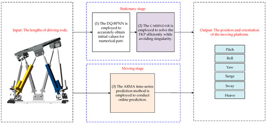
Figure 1.
The overview of the proposed method.
- (1)
- The DQ-BPNN is employed to accurately acquire initial values for the numerical part. The DQ-BPNN demonstrates a superior fitting effect with a wide range of inputs and is integrated with the ResNet to capture deeper-level system characteristics. Leveraging the advantages of dual quaternions, the DQ-BPNN is characterized by higher efficiency and a unified representation form.
- (2)
- The C-MSFND-NR is employed to solve the FKP efficiently while avoiding singularity. This C-MSFND-NR exhibits higher computing efficiency, enhanced convergence stability, and the capacity to address the singularity issue of the Jacobian matrix.
- (3)
- The ARMA time-series prediction method is employed to conduct online prediction. A traversal method is adopted to determine the order of the ARMA model. This approach enables real-time and highly accurate prediction of the Stewart platform’s pose.
3. The Mathematical Model of the Stewart Platform
The Stewart platform consists of a moving platform, a fixed platform, upper hinge assemblies, lower hinge assemblies and actuators.
3.1. Structural and Kinematic Characteristics of the Stewart Platform in Forward Kinematics
The general Stewart platform has five structural parameters as shown in Figure 2, the moving and fixed platform radii and , the angle and , and the distance between the moving and fixed platforms is when the Stewart platform is in the initial assembly configuration.
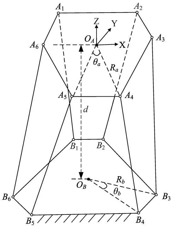
Figure 2.
The spatial position relationships of joint points in Stewart platform.
In Figure 3, the geometric structure reveals that , and . The spatial position relationships of joint points in the Stewart platform show that the hinge points on the moving platform are positioned on a circle. Similarly, the hinge points on the fixed platform are also located on a circle.
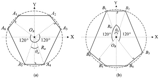
Figure 3.
(a) The moving platform; (b) the fixed platform.
The position and orientation of the moving platform are denoted as the vector . R denotes the rotation matrix within the Euler angle scheme ( for Pitch, for Roll, and for Yaw), which is elaborated as follows.
The coordinates of the joint points on the moving platform and the fixed platform are denoted as and ( = 1, 2, …, 6), which are measured in the base frame. The six actuator vectors Li (i = 1,2, …, 6) can be expressed as follows.
3.2. The Properties of Dual Quaternions
Rigid-body rotation techniques involve direction cosines and quaternions. Direction cosines require nine parameters, while quaternions need only four, making quaternions more concise. Compared with direction-cosine-based methods, quaternions significantly reduce trigonometric calculation complexity [37]. Dual quaternions offer a unified and efficient way to describe full rigid-body motion, simplifying computations and providing a more straightforward approach than direction cosines. A dual quaternion, a mathematical entity with eight elements, has both real and dual components, similar to quaternions. Unlike standard quaternions that can only represent spatial rotations, dual quaternions can describe any combination of spatial rotation and translation.
and form a dual quaternion .
where is a dual unit, and . In this context, , .
The homogeneous transformation matrix T can be expressed by dual quaternions as follows:
3.3. Two Scenarios Where FKP Diverges
In the FKP of the Stewart platform, two distinct singular scenarios emerge. The first scenario is characterized by the divergence of the Newton–Raphson method, resulting from inappropriately selected initial values. Those inappropriate initial values cause the iterative process to deviate from convergence, leading to non-reliable numerical outcomes.
In the Newton–Raphson method, the solution at the current step and the solution at the next computational step are denoted as and , respectively, while the true value is represented as . As can be clearly seen from Figure 4, the initial iteration values are poorly selected. When the initial iteration values are inadequately chosen and fail to approximate the actual root of the target function, incorrect results for both the current and subsequent solutions are inevitable.
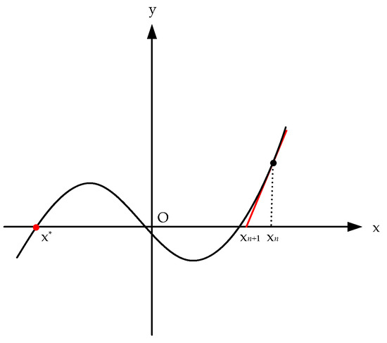
Figure 4.
The first singular scenario of FKP in the Stewart platform.
The second scenario involves the singularity of the Jacobian matrix. Specifically, this manifests when the maximum condition number of the Jacobian matrix, which is computed as the ratio of the maximum singular value to the minimum singular value of the Jacobian matrix, exceeds an acceptable threshold. A large condition number indicates a high level of numerical sensitivity within the matrix, potentially leading to instabilities in the kinematic analysis.
The maximum and minimum singular values of the Jacobian matrix are and . As presented below, represents the condition number and serves as an indicator for judging whether the Jacobian matrix is singular.
In the left part of Figure 5, the sphere indicates that the maximum and minimum singular values of the Jacobian matrix are equal. Conversely, in the right part of Figure 5, the ellipse indicates that the maximum singular value of the Jacobian matrix is notably greater than the minimum one. This significant difference gives rise to a greater degree of singularity in the Jacobian matrix. Additionally, an excessively large value of indicates the occurrence of singularity. In such a case, renewing the Jacobian matrix becomes necessary to avoid singularity.
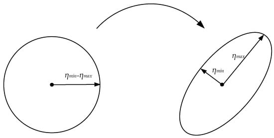
Figure 5.
The second singular scenario of FKP in the Stewart platform.
4. Hybrid Algorithm for FKP in the Stewart Platform
The hybrid algorithm for FKP in the Stewart platform is divided into two stages: the stationary stage and the moving stage.
As depicted in Figure 6, during the stationary stage of solving the FKP, the DQ- BPNN is initially utilized. Subsequently, the C-MSFND-NR is applied following the utilization of the DQ-BPNN.
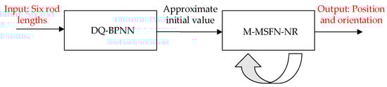
Figure 6.
The stationary stage of the FKP.
As depicted in Figure 7, during the moving stage of solving the FKP, the ARMA algorithm is the first to be applied for time-series prediction. Meanwhile, the Newton–Raphson method is used in iterative computations.
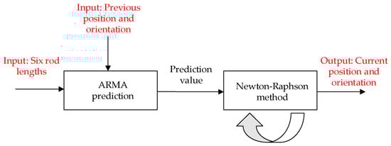
Figure 7.
The moving stage of the FKP.
4.1. The DQ-BPNN with More Features and Integrated with the ResNet
The DQ-BPNN is trained with a large number of data samples randomly generated within the range of the minimum and maximum positions and orientation values. Notably, it only needs to be trained once to be applicable to all scenarios.
The length of the driving rod is ( = 1, 2, …, 6), and the DQ-BPNN has 12 input variables, including the lengths of different driving rods, maximum length, minimum length, cumulative length, average length, length range, and the average difference in length of the six driving rods. The output is constituted by the dual quaternions related to the position and orientation of the moving platform. The 12 input variables include ( = 1, 2, …, 6), , , , , , ., among the previously mentioned elements.
Employing 12 variables rather than 6 enables the DQ-BPNN to achieve an alternative fitting effect. This is because a larger number of parameters can capture more features. The position and orientation of the mobile platform can be calculated based on the output of the DQ-BPNN. The input comprises 12-dimensional input associated with the lengths of the six driving rods, while the output consists of the real part and the dual part of the DQ-BPNN. The real part of DQ-BPNN implies that, given a 12-dimensional input, the output is an attitude-related quaternion, while the dual part indicates an orientation-related quaternion output. The schematic diagram of DQ-BPNN is shown in Figure 8.
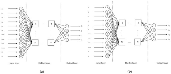
Figure 8.
The schematic diagram of DQ-BPNN. (a) The real part of DQ-BPNN; (b) the dual part of DQ-BPNN.
The ResNet addresses the problems of gradient-vanishing and degradation, enhancing feature extraction capabilities and model generalization. ResNet integrates skip connections, which are crucial for seamless gradient spread across the network. This integration enables neural networks to train deeper models more effectively. In Figure 9, the symbol denotes the input variable, while represents the output function. Notably, tanh is adopted as the activation function here.
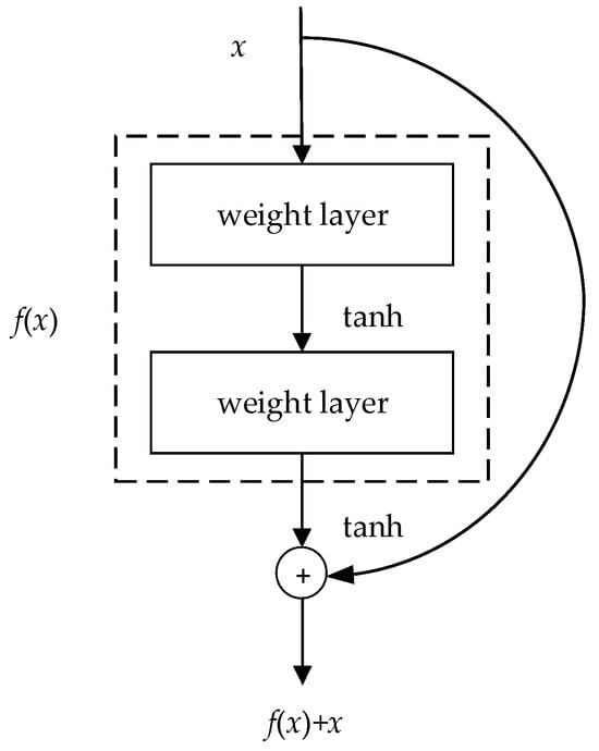
Figure 9.
The schematic diagram of ResNet.
4.2. The C-MSFND-NR Method with High Efficiency and the Capability to Resolve Jacobian Matrix
In this section, the work proposes the C-MSFND-NR to obtain high efficiency and the capability to resolve Jacobian matrix. The existing methods are the Newton–Raphson method and Newton downhill method. The Newton–Raphson method, with the prominent advantage of second-order convergence, is of vital importance in solving nonlinear equation systems. Despite its rapid convergence, the Newton–Raphson method exhibits high sensitivity to the selection of initial values and has a relatively confined convergence range. The Newton downhill method converges rapidly in the vicinity of the optimal solution by leveraging second-order derivative information. However, the determination of the downhill step length and scale factor requires careful consideration, as incorrect values will have a negative impact on the algorithm’s performance. At the same time, neither the Newton–Raphson method nor the Newton downhill method can resolve the singularity problem in the Jacobian matrix.
To enhance both the efficiency and numerical stability in the FKP, this work proposes the C-MSFND-NR method based on dual quaternions. This method not only integrates the merits of the Newton–Raphson method and the Newton downhill method, but also has the capacity to resolve singular matrices. Furthermore, in C-MSFND-NR, a genetic algorithm is introduced for fine-tuning the algorithm parameters. These parameters include the iteration number of the Newton downhill method stage, the initial value of the step matrix, and the scaling factor matrix.
Lv et al. [38] presented a modification of the Newtonian method solving non-linear equations with singular Jacobian, and the two Newtonian methods are called predictor–corrector modification (PC-M) and quadrature-based predictor–corrector modification (QMn-M).
- Newton–Raphson method.
As depicted in Ref. [19], the iterative sequence is
where the Jacobian matrix is an 8 × 8 square matrix, and and are 8 × 1 column vectors, and are the equations of FKP.
- Quasi-Newton method.
- The iterative sequence is
- Newton downhill method.
The iterative sequence is
where is the descent factor. When , Newton downhill method is converted into the Newton–Raphson method. When , remains the same. Conversely, .
- C-MSFND-NR method.
The iterative sequence is
where is the downhill factor in C-MSFND-NR, is the Newton downhill iteration number in C-MSFND-NR. is calculated as follows.
where is the scale factor matrix of . When , is equal to and remains the same. Conversely, , where t is the number of iterations until in the kth solution process.
When the Jacobian matrix is singular, is updated by Equation (13).
where is the coefficient of the diagonal matrix. A diagonal matrix multiplied by a coefficient is incorporated into the singular Jacobian matrix to modify the non-invertible characteristics of the Jacobian matrix in the iterative process. Moreover, that algorithm exhibits second-order convergence.
Since the step size matrix , the scale factor matrix w, and the iteration number of C-MSFND-NR directly influence the convergence range and convergence speed of the algorithm, the genetic algorithm is utilized to optimize those parameters to achieve better computing efficiency. The optimization formula is shown in Equation (14).
where is the total calculation time. and are the downhill step length and scale factor in C-MSFND-NR.
Figure 10 and Figure 11 present the workflow of the C-MSFND-NR. Figure 10 shows the offline genetic algorithm stage, and Figure 11 shows the online Newton downhill and Newton–Raphson method stages.
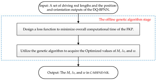
Figure 10.
The offline genetic algorithm stage in the C-MSFND-NR.
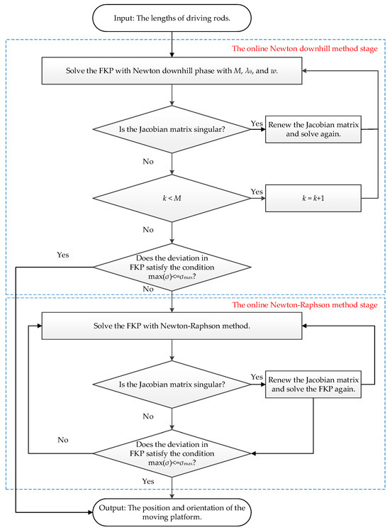
Figure 11.
The online Newton downhill and Newton–Raphson method stages in the C-MSFND-NR.
Firstly, in the offline genetic algorithm stage presented in Figure 10, the genetic algorithm is applied to optimize the coefficients of the C-MSFND-NR. Minimizing the total computation time is defined as the optimization objective function. This function takes as inputs a set of driving rod lengths and the position-and-orientation outputs of the DQ-BPNN. The data set, which is representative of all situations, enables the coefficients to be applied universally and calculated only once.
Secondly, during the online Newton downhill method stage, the algorithm executes a maximum of M times. When the Jacobian matrix is singular, a new matrix will be generated. Finally, in the stage of the online Newton–Raphson method, this method is employed to swiftly solve the FKP. Simultaneously, and represent the actual and maximum deviations in the FKP, respectively.
4.3. The ARMA Approach for Online Time-Series Forecasting
Generally, DQ-BPNN primarily facilitates initial value setting in numerical solutions, emphasizing data’s non-linear features and spatial relations. In contrast, ARMA is mainly applied to time-series prediction, highlighting data’s change patterns and linear relations in the time domain. These two methods logically complement one another, jointly constituting the hybrid strategy for solving the Stewart platform’s forward kinematics. There is no need to obtain the initial value for the FKP using the DQ-BPNN every time. Once the actual position and orientation values are initially determined, the ARMA method can be applied to obtain the initial value for the numerical method. This consequently reduces the time required for FKP calculation.
Typically, to enhance computational efficiency and minimize the number of iterations, the FKP for the Stewart platform commonly employs the outcome of the preceding iteration as the initial value. In cases where this is not applicable, the FKP makes use of the linear method described in Equation (15) for computation.
where represents the pose data at the previous moment, denotes the speed of the previous pose, and stands for the time interval between two consecutive control cycles.
However, the estimated values derived from the linear method remain insufficiently accurate. This inaccuracy directly impacts the number of iterations and calculation time in subsequent numerical calculations. Consequently, the ARMA method is employed to accurately predict the initial values of FKP in real time.
The model consists of two components: the component and the component. In the AR component, denotes the number of autoregressive terms, signifying that historical data of the sequence itself is utilized to forecast future values. In the MA component, represents the number of moving average terms, indicating that fitting errors are employed to predict future values.
where denotes a constant term. , ..., represent the actual poses at the previous moments. and are autoregressive coefficients. and the deviations at the previous moments, and and are the moving average coefficients.
The Bayesian Information Criterion (BIC) is employed to explore different combinations of p and q. While guaranteeing sufficient accuracy of the predicted poses, the model parameters corresponding to the minimum BIC value are identified. The definition formula for the BIC is given as follows.
where is the maximum likelihood estimate of the model, which indicates the goodness-of-fit to the data. is the number of estimable parameters in the model, reflecting the complexity of the model. is the sample size, denoting the number of data points utilized for model fitting.
During the operation of the Stewart platform, maintaining an accurate ARMA model is crucial. Accurate predictions play a vital role in enabling precise control and ensuring the smooth operation of the platform. Simultaneously, minimizing the BIC value is highly significant. A lower BIC value aids in the selection of the most suitable ARMA model, preventing overfitting and enhancing the overall performance.
5. Simulations and Experiments
The offline computation is executed on a computer system equipped with an i9-13980HX processor (Intel, Santa Clara, CA, USA). This processor has a maximum turbo-boost frequency of up to 5.6 GHz and is paired with 32 GB of RAM. Additionally, the training process employs the desktop-edition RTX 4080 GPU (Graphics Processing Unit).
The equipment YBT6-250 was sourced from Wuhan Huazhiyang Technology Co., Ltd. The company is located in Wuhan, China.
The experimental Stewart platform YBT6-250 is presented in Figure 12. For this platform, = 565.413 mm, = 747.69 mm, = 16.268°, = 13.056°, and = 1024.180 mm.
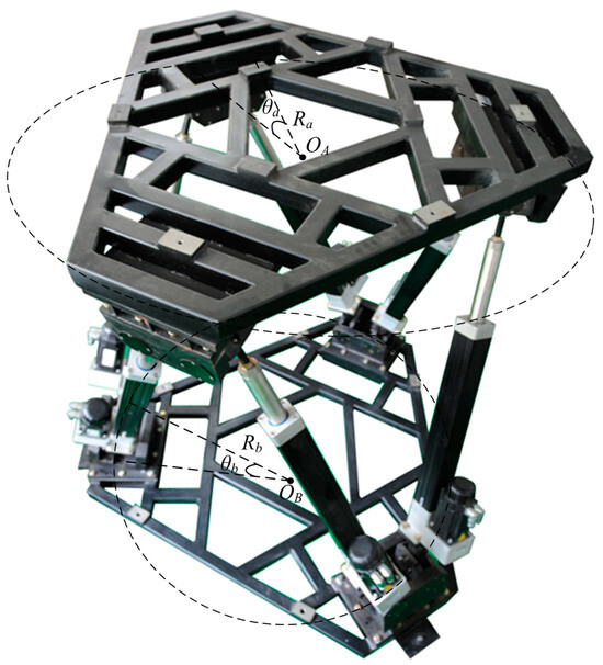
Figure 12.
The experimental Stewart platform.
5.1. Experimental Design and Condition
The coordinates of hinge points on the moving and fixed platforms are listed in Table 2.
Table 2.
Coordinates of hinge points on the moving and fixed platforms (units: mm).
For different positions and orientations, the following metrics are calculated within the test set of the neural network: the coefficient of multiple determination (R2), mean absolute error (MAE), mean absolute percentage error (MAPE), root mean square error (RMSE), and mean square error (MSE). In Equations (18)–(22), (i = 1, 2, …, n) represents the actual value in the test set, is the average value of , and denotes the predicted values derived from the neural network.
5.2. Experimental Results and Analysis
When the Stewart platform is in neutral position, the length of the drive rod is 1154.708 mm.
A total of 4096 data samples are randomly generated within the range of the minimum and maximum positions and orientation values. Additionally, 729 sets of samples are designated for testing. The maximum and minimum orientations are 85° and −85°, respectively, while the maximum and minimum position values are 300 mm and −300 mm, respectively.
Table 3 shows the coefficients in C-MSFND-NR model obtained by genetic algorithm.
Table 3.
The coefficients in C-MSFND-NR.
Table 4 presents a comparison of various numerical algorithms for resolving a singular matrix when dealing with different initial position and orientation values for the FKP. Specifically, three cases are examined in this table. Evidently, the Newton–Raphson method, Quasi-Newton method, and Newton downhill method are incapable of handling the singular Jacobian matrix. In contrast, the PC-M, QMn-M, and C-MSFND-NR algorithms can resolve the singular Jacobian matrix and accurately obtain the correct results for the FKP.
Table 4.
Comparison of various numerical algorithms to resolve a singular matrix.
Command the Stewart platform to execute a 5-degree amplitude, 6 s duration sine oscillation on each of the pitch, roll, and yaw axes. Also, command the Stewart platform to perform a 10 mm amplitude, 6 s period sine motion on each of the surge, sway, and heave axes. Record the real-time pose and use the ARMA algorithm to find the order of the recorded data. The coefficients of ARMA model are shown in Table 5.
Table 5.
The coefficients of ARMA model.
5.3. Comparison of Computational Efficiency and Accuracy
The computational time for processing 10,000 sampled points, with a sampling period of 10 milliseconds and each forward kinematics problem (FKP) calculation initiated from an initial value of zero, is presented below. Remarkably, the results demonstrate that the application of dual quaternions yields a 59.52% enhancement in computational efficiency when compared with spatial cosine matrices.
Table 6 presents a comparison of the computational efficiency between dual quaternions and spatial cosine matrices. In a scenario, the Stewart platform performs a 10-degree amplitude, 10 s period sinusoidal roll, while other position and orientation parameters stay zero. The computational time for processing 10,000 sample points, with a sampling period of 10 milliseconds and each forward kinematics problem (FKP) calculation initiated from the initial value of zero, is presented below. Remarkably, the results demonstrate that the application of dual quaternions yields a 59.52% enhancement in computational efficiency when compared with spatial cosine matrices.
Table 6.
Computational efficiency comparison of dual quaternions with spatial cosine matrices.
Table 7 shows that the R2 in DQ-BPNN increases by 0.1% when compared with that in BPNN. Meanwhile, MAE, MAPE RMSE, and MSE in DQ-BPNN decrease by 8.89%, 21.85%, 6.90%, 3.3% when compared with those in BPNN.
Table 7.
Comparison of five metrics regarding accuracy on the test set.
As shown by the data in Table 8, the C-MSFND-NR outperforms other methods. When compared with the Newton–Raphson method, Quasi-Newton method, Newton downhill method, PC-M method, and QMn-M method, the average number of iterations of the C-MSFND-NR method decreases by 50.30%, 50.30%, remains unchanged, 50.30%, 50.30%. Moreover, the average computing time of the C-MSFND-NR method decreases by 59.82%, 83.81%, 15.09%, 79.82%, and 78.77%, respectively.
Table 8.
Comparing computational efficiency of algorithms for FKP in the test set.
Figure 13 shows the comparison of iteration number among different Newtonian methods.
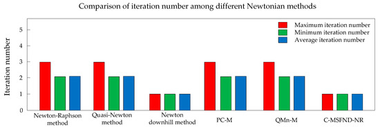
Figure 13.
Comparison of iteration number among different Newtonian methods.
Figure 14 shows the comparison of iteration time among different Newtonian methods.
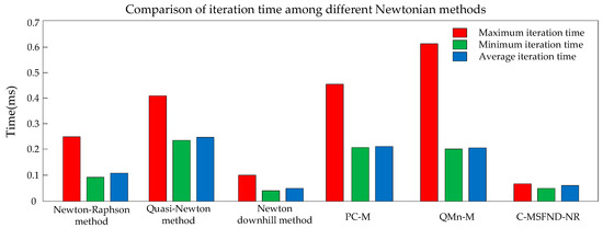
Figure 14.
Comparison of iteration time among different Newtonian methods.
Table 9 compares the maximum deviation in time-series prediction between the linear method and the ARMA method. In comparison to the linear method, the prediction accuracy of the ARMA method has increased by 14.63%, 14.63%, 14.63%, 14.46%, 16.67%, and 13.41%, respectively.
Table 9.
Comparison of maximum deviation between the linear method and the ARMA method.
Figure 15 shows that the ARMA method exhibits greater precision compared with the linear method. In this scenario, the Stewart platform executes sine oscillations along the pitch, roll, and yaw axes. Each oscillation has an amplitude of 5 degrees and a duration of 6 s. Additionally, the platform performs sine motions along the surge, sway, and heave axes, with each motion having an amplitude of 10 mm and a period of 6 s.
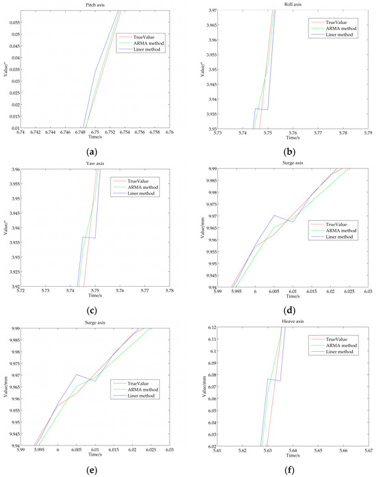
Figure 15.
Precision comparison between the ARMA method and the linear method. (a) Pitch axis; (b) roll axis; (c) yaw axis; (d) surge axis; (e) sway axis; (f) heave axis.
Owing to the high accuracy of the ARMA algorithm, in most cases, a single iteration of the Newton–Raphson method suffices to achieve the specified accuracy.
6. Conclusions
To overcome the deficiencies of computational precision, efficiency, the capacity to resolve singular Jacobian matrix, and real-time prediction of the position and orientation in the existing methods, this work proposes a hybrid strategy for forward kinematics in the Stewart platform based on dual quaternion neural network and ARMA time series prediction. Firstly, this work proposes the DQ-BPNN for FKP in the Stewart platform. The DQ-BPNN that employs dual quaternions exhibits higher computational efficiency and a more compact structure compared with the approach using spatial cosine matrices. The integration of supplementary features related to rod lengths, along with the implementation of the ResNet, gives rise to a remarkable improvement in the global fitting accuracy of the neural network. Secondly, this work proposes C-MSFND-NR. The C-MSFND-NR not only remarkably enhances efficiency, but also possesses the ability to resolve the singularity within the Jacobian matrix. Finally, this work employs the ARMA method to conduct real-time prediction of the position and orientation during motion, thereby significantly improving the efficiency in FKP.
When compared with previous algorithms for solving the FKP, the proposed method presents the following advantages: (1) The accuracy of the DQ-BPNN surpasses that of traditional BPNN methods. Moreover, the DQ-BPNN, which utilizes dual quaternions, not only exhibits higher fitting accuracy and computational efficiency in solving the FKP, but also features a more compact structure compared with the approach employing spatial cosine matrices. (2) The C-MSFND-NR provides enhanced efficiency and has greater capacity to resolve the singularity of the Jacobian matrix than other numerical methods. (3) The ARMA method exhibits a superior fitting effect than the linear method when conducting real-time prediction of the position and orientation during motion.
The simulations and experiments indicate that, in comparison with the BPNN, the R2 value in DQ-BPNN increases by 0.1%. Meanwhile, the MAE, MAPE, RMSE, and MSE values of the DQ-BPNN decrease by 8.89%, 21.85%, 6.90%, and 3.3%, respectively. When compared with five Newtonian methods, the average computing time of C-MSFND-NR algorithm decreases by 59.82%, 83.81%, 15.09%, 79.82%, and 78.77%. In comparison to the linear method, the prediction accuracy of the ARMA method increases by 14.63%, 14.63%, 14.63%, 14.46%, 16.67%, and 13.41%, respectively.
Author Contributions
Conceptualization, J.T.; methodology, J.T.; software, J.T.; validation, J.T.; formal analysis, J.T.; investigation, W.F.; resources, J.T.; data curation, J.T.; writing—original draft preparation, J.T.; writing—review and editing, W.F.; visualization, J.T.; supervision, W.F.; project administration, H.Z. All authors have read and agreed to the published version of the manuscript.
Funding
This research was funded by Research on Key Technologies of High-Performance CNC System Product Package (2023BAA010-1).
Data Availability Statement
Data are contained within the article.
Conflicts of Interest
The authors declare no conflicts of interest.
References
- He, Z.; Feng, X.; Zhu, Y.; Yu, Z.; Li, Z.; Zhang, Y.; Wang, Y.; Wang, P.; Zhao, L. Progress of Stewart Vibration Platform in Aerospace Micro–Vibration Control. Aerospace 2022, 9, 324. [Google Scholar] [CrossRef]
- Wei, M.-Y.; Fang, S.-A.; Liu, J.-W. Design and Implementation of a New Training Flight Simulator System. Sensors 2022, 22, 7933. [Google Scholar] [CrossRef] [PubMed]
- Cetin, K.; Tugal, H.; Petillot, Y.; Dunnigan, M.; Newbrook, L.; Erden, M.S. A Robotic Experimental Setup with a Stewart Platform to Emulate Underwater Vehicle-Manipulator Systems. Sensors 2022, 22, 5827. [Google Scholar] [CrossRef] [PubMed]
- Huang, X.; Liao, Q.; Wei, S. Closed-form forward kinematics for a symmetrical 6-6 Stewart platform using algebraic elimination. Mech. Mach. Theory 2010, 45, 327–334. [Google Scholar]
- Nag, A.; Vellanchola, S.; Bandyopadhyay, S. A uniform geometric-algebraic framework for the forward kinematic analysis of 6-6 stewart platform manipulators of various architectures and other related 6-6 spatial manipulators. Mech. Mach. Theory 2021, 155, 104090. [Google Scholar]
- Lee, T.Y.; Shim, J.K. Forward kinematics of the general 6-6 Stewart platform using algebraic elimination. Mech. Mach. Theory 2001, 36, 1073–1085. [Google Scholar]
- Wampler, C.W. Forward displacement analysis of general six-in-parallel SPS (Stewart) platform manipulators using soma coordinates. Mech. Mach. Theory 1996, 31, 331–337. [Google Scholar]
- Faugère, J.C.; Lazard, D. Combinatorial classes of parallel manipulators. Mech. Mach. Theory 1995, 30, 765–776. [Google Scholar]
- Wei, F.; Wei, S.; Zhang, Y. Algebraic solution for the forward displacement analysis of the general 6-6 stewart mechanism. Chin. J. Mech. Eng. 2016, 29, 56–62. [Google Scholar]
- Zhang, Y.; Liao, Q.; Wei, S.; Wei, F. A Unified Algorithm for the Forward Displacement Analysis of In-parallel Stewart-Gough Platforms. In Proceedings of the 14th IFToMM World Congress, Taipei, Taiwan, 25–30 October 2015; pp. 100–107. [Google Scholar]
- Raghavan, M. The Stewart platform of general geometry has 40 configurations. AMSE J. Mech. Des. 1993, 115, 277–282. [Google Scholar]
- Sadjadian, H.; Taghirad, H.D. Numerical methods for computing the forward kinematics of a redundant parallel manipulator. In Proceedings of the IEEE Conference on Mechatronics and Robotics, Aachen, Germany, 13–15 September 2004; pp. 557–562. [Google Scholar]
- Merlet, J.P. Solving the forward kinematics of a Gough-type parallel manipulator with interval analysis. Int. J. Robot. Res. 2004, 23, 221–235. [Google Scholar]
- Yang, X.; Wu, H.; Chen, B.; Zhu, L.; Xun, J. Fast numerical solution to forward kinematics of general Stewart mechanism using quaternion. Trans. Nanjing Univ. Aeronaut. Astronaut. 2014, 31, 377–385. [Google Scholar]
- Merlet, J.P. Direct kinematics of parallel manipulators. IEEE Trans. Robot. Autom. 1993, 9, 842–846. [Google Scholar]
- Yang, C.F.; Zheng, S.T.; Jin, J.; Zhu, S.B.; Han, J.W. Forward kinematics analysis of parallel manipulator using modified global Newton-Raphson method. J. Cent. South Univ. Technol. 2010, 17, 1264–1270. [Google Scholar]
- Puglisi, L.J.; Saltaren, P.R.J.; Garcia, C.; Cecilia, E.C.; Pedro, F.M.; Hector, A. Implementation of a generic constraint function to solve the direct kinematics of parallel manipulators using Newton-Raphson approach. J. Control Eng. Appl. Inf. 2017, 19, 71–79. [Google Scholar]
- Liu, K.; Lewis, F.L.; Fitzgerald, M. Solution of nonlinear kinematics of a parallel-link constrained Stewart platform manipulator. Circuits Syst. Signal Process. 1994, 13, 167–183. [Google Scholar]
- Yang, X.; Wu, H.; Li, Y. A dual quaternion solution to the forward kinematics of a class of six-DOF parallel robots with full or reductant actuation. Mech. Mach. Theory 2017, 107, 27–36. [Google Scholar]
- Zhou, W.; Chen, W.; Liu, H. A new forward kinematic algorithm for a general Stewart platform. Mech. Mach. Theory 2015, 87, 177–190. [Google Scholar]
- Yang, C.; He, J.; Han, J.; Liu, X. Real-time state estimation for spatial 6-DOF linearly actuated parallel robots. Mechatronics 2009, 19, 1026–1033. [Google Scholar]
- Wang, Z.; He, J.; Shang, H.; Gu, H. Forward Kinematics Analysis of a Six-DOF Stewart Platform Using PCA and NM Algorithm. Ind. Robot 2009, 36, 448–460. [Google Scholar]
- Yang, F.; Tan, X.; Wang, Z.; Lu, Z.; He, T. A Geometric Approach for Real-Time Forward Kinematics of the General Stewart Platform. Sensors 2022, 22, 4829. [Google Scholar] [CrossRef] [PubMed]
- Bonev, I.A.; Ryu, J. A new method for solving the direct kinematics of general 6-6 Stewart Platforms using three linear extra sensors. Mech. Mach. Theory 2000, 35, 423–436. [Google Scholar]
- Kim, J.S.; Jeong, Y.H.; Park, J.H. A geometric approach for forward kinematics analysis of a 3-SPS/S redundant motion manipulator with an extra sensor using conformal geometric algebra. Meccanica 2016, 51, 2289–2304. [Google Scholar]
- Mahmoodi, A.; Sayadi, A.; Menhaj, M.B. Solution of forward kinematics in Stewart platform using six rotary sensors on joints of three legs. Adv. Robot. 2014, 28, 27–37. [Google Scholar]
- Yee, C.s.; Lim, K.b. Forward kinematics solution of Stewart platform using neural networks. Neurocomputing 1997, 16, 333–349. [Google Scholar]
- Faraji, H.; Rezvani, K.; Hajimirzaalian, H.; Hossein, M. Solving the Forward Kinematics Problem in Parallel Manipulators Using Neural Network. In Proceedings of the 2017 5th International Conference on Control, Mechatronics and Automation, ICCMA 2017, Beijing, China, 11 October 2017; pp. 23–29. [Google Scholar]
- Morell, A.; Tarokh, M.; Acosta, L. Solving the forward kinematics problem in parallel robots using Support Vector Regression. Eng. Appl. Artif. Intell. 2013, 26, 1698–1706. [Google Scholar]
- Limtrakul, S.; Arnonkijpanich, B. Supervised learning based on the self-organizing maps for forward kinematic modeling of Stewart platform. Neural Comput. Appl. 2019, 31, 619–635. [Google Scholar]
- Parikh, P.J.; Lam, S.S.Y. A hybrid strategy to solve the forward kinematics problem in parallel manipulators. IEEE Trans. Robot. 2005, 21, 18–25. [Google Scholar]
- Zhu, H.; Xu, W.; Yu, B.; Ding, F.; Cheng, L.; Huang, J. A Novel Hybrid Algorithm for the Forward Kinematics Problem of 6 DOF Based on Neural Networks. Sensors 2022, 22, 5318. [Google Scholar] [CrossRef]
- Morell, A.; Acosta, L.; Toledo, J. An artificial intelligence approach to forward kinematics of Stewart platforms. In Proceedings of the 2012 20th Mediterranean Conference on Control & Automation (MED), Barcelona, Spain, 3–6 July 2012; pp. 433–438. [Google Scholar]
- Parikh, P.J.; Lam, S.S. Solving the forward kinematics problem in parallel manipulators using an iterative artificial neural network strategy. Int. J. Adv. Manuf. Technol. 2009, 40, 595–606. [Google Scholar]
- Zhu, Q.; Zhang, Z. An efficient numerical method for forward kinematics of parallel robots. IEEE Access 2019, 7, 128758–128766. [Google Scholar] [CrossRef]
- Yin, Z.; Qin, R.; Liu, Y. A New Solving Method Based on Simulated Annealing Particle Swarm Optimization for the Forward Kinematic Problem of the Stewart–Gough Platform. Appl. Sci. 2022, 12, 7657. [Google Scholar] [CrossRef]
- Tao, J.; Zhou, H.; Fan, W. Efficient and High-Precision Method of Calculating Maximum Singularity-Free Space in Stewart Platform Based on K-Means Clustering and CNN-LSTM-Attention Model. Actuators 2025, 14, 74. [Google Scholar] [CrossRef]
- Lv, W.; Wei, L.T.; Feng, E.M. A modification of Newton’s method solving non-linear equations with singular Jacobian. Kongzhi Juece Control Decis. 2017, 32, 2240–2246. [Google Scholar]
Disclaimer/Publisher’s Note: The statements, opinions and data contained in all publications are solely those of the individual author(s) and contributor(s) and not of MDPI and/or the editor(s). MDPI and/or the editor(s) disclaim responsibility for any injury to people or property resulting from any ideas, methods, instructions or products referred to in the content. |
© 2025 by the authors. Licensee MDPI, Basel, Switzerland. This article is an open access article distributed under the terms and conditions of the Creative Commons Attribution (CC BY) license (https://creativecommons.org/licenses/by/4.0/).