Prescribed-Time-Based Anti-Disturbance Tracking Control of Manipulators Under Multiple Constraints

Abstract

Manipulators have a wide range of applications in industrial automation. However, their nonlinear characteristics, time-varying properties, and external disturbances present significant challenges in accurately tracking their trajectories. This paper proposes an integrated control strategy based on prescribed-time convergence control, output constraint control, prescribed performance control (PPC), and an extended state observer (ESO)-based anti-disturbance control method. The prescribed-time convergence control guarantees that the system will reach a steady state at a specified time, while the output constraint control ensures that the Vm will move within a predefined physical range. The PPC meets the rigorous requirements of error convergence during trajectory tracking by regulating the error dynamics, while the ESO is employed to estimate unknown disturbances and enhance the system’s resilience to interference. The simulation outcomes demonstrate that the proposed control methodology exhibits notable advantages in terms of a rapid response, precision tracking, and anti-disturbance capabilities.

1. Introduction

Manipulators are employed in a multitude of fields, including engineering, manufacturing automation, and aerospace, due to their high power density, stability, and reliability [1,2,3]. In these application scenarios, trajectory tracking control represents a fundamental technology for the realization of automated operations. However, the control of manipulators presents a number of significant challenges. The inherent nonlinearity and time-varying nature of systems, coupled with the influence of external environmental disturbances, often result in traditional control methods failing to achieve an optimal balance between accuracy, response speed, and anti-disturbance capabilities. Consequently, there is considerable theoretical value and practical significance in studying control strategies that can enhance the trajectory tracking performance in complex environments [4]. Despite the continued use of traditional control methods, such as proportional–integral–derivative (PID) controllers, there is increasing recognition of their inadequacy to address the challenges posed by the complexity of nonlinear systems and external disturbances. To address these challenges in manipulator control, researchers have integrated PID control with advanced control techniques to compensate for the limitations of traditional PID control. For instance, the neural network-based optimization of the PID controller has been proposed for supersonic unmanned aerial vehicle (UAV) trajectory tracking, leading to substantial enhancements in accuracy. Meanwhile, refs. [5,6] presents a fuzzy gain scheduling PID strategy for a multi-stage UAV mission, effectively addressing time-varying requirements. In contrast, a range of advanced techniques grounded in contemporary control theory have emerged in recent years. These techniques include ESO-based prescribed-time convergence control, output-constrained control, PPC, and anti-disturbance control. Each approach offers unique advantages and can improve systems’ performance to varying degrees.

In contrast to finite-time control and fixed-time control, the convergence time of prescribed-time control is not constrained by the design parameters and initial state; instead, it is predetermined by human beings, and its control algorithm is straightforward, with a smooth control signal. In [7,8], the authors apply the theory of prescribed-time control to the stabilization control of uncertain nonlinear systems, combining adaptive and backstepping control to design a new feedback controller that ensures the prescribed-time convergence of the system. Meanwhile, ref. [9] proposes a new prescribed-time distributed consensus and containment control algorithm for the generalization of prescribed-time control to multi-agent systems. When considering multi-agent systems, time synchronization becomes crucial in maintaining formation accuracy. Consensus-based control strategies with dynamic time synchronization mechanisms have proven effective in decentralized robot groups, particularly in military logistics scenarios requiring precise coordination [10]. The prescribed-time control algorithm addresses the issue of slow response times in manipulators by developing suitable control laws to guarantee that the system state is stabilized within a specified time frame. In comparison to the asymptotic convergence method, prescribed-time convergence control has the potential to markedly enhance both the rapidity and stability of the system, particularly in scenarios where dynamic changes occur rapidly. The nonlinearity and uncertainty inherent in manipulators render traditional controllers incapable of accurately predicting the convergence times.

Manipulators are typically constrained by physical boundaries, including joint angles, velocities, and accelerations, during operation. The objective of output constraint control is to guarantee that the system output (e.g., position and velocity) remains within predefined constraints. This control method ensures that the trajectories of the manipulators do not violate the physical constraints, thus enhancing the safety and stability of the system. In order to implement output constraint control, a barrier Lyapunov function (BLF) is typically constructed to guarantee that the system does not exceed the constraint range during trajectory tracking [11]. This approach is especially crucial in the motion control of manipulators, as exceeding the physical constraints may result in mechanical damage or operational failures. In [12], the authors employ the combination of a fixed-time disturbance observer, sliding-mode control, and a BLF, thereby achieving the full-state constraint motion control of a space robotic manipulator. A full-state constrained tracking controller based on non-singular terminal sliding modes and BLF has been designed for robot manipulators in [13].

PPC is a control strategy that ensures that the prescribed performance requirements of a system are met by imposing a performance inclusion function [14]. PPC ensures that the system error quickly converges to within a specified range in a given time by designing an error convergence function. This control method enables the controller to maintain optimal performance metrics during dynamic changes, making it particularly well suited for tasks requiring precise trajectory tracking. In the control of manipulators, PPC can provide a well-defined range and speed of convergence for the error dynamic design, thereby avoiding the problem of error accumulation that may occur in traditional methods. Furthermore, PPC is able to provide high-performance tracking throughout the motion process through strict constraints on the error, which is a significant advantage, especially in scenarios requiring high-precision tracking. In order to achieve transient and steady-state performance, ref. [15] has designed an adaptive prescribed performance tracking controller based on a radial basis function neural network for a class of n-degree-of-freedom (DOF) manipulators. A tracking controller for a two-DOF manipulator driven by an electrohydraulic actuator has been proposed by combining adaptive neural networks and PPC, as detailed in [16].

It is not uncommon for external disturbances and modeling inaccuracies to be present in the control systems of manipulators. Such uncertainties have the potential to lead to the degradation of the system’s performance. The ESO represents an effective tool for the estimation of the unmodeled dynamics of the system and external disturbances. The robustness of the system can be markedly enhanced by monitoring the disturbance information of the system in real time through the ESO and incorporating these data into the control law. As evidenced in [17], the ESO is an effective tool for the estimation of external disturbances and uncertainties in complex systems. By compensating for these total disturbances, the ESO can enhance the control accuracy and anti-disturbance performance of the system. In the context of manipulator control, the ESO is a widely utilized technique in improving the robustness of systems, particularly in complex operating environments. Its implementation can lead to notable improvements in system stability and accuracy. Ref. [18] designed an adaptive robust tracking controller based on a dual ESO for a multi-DOF manipulator with unknown uncertainties and external disturbances. The incorporation of a fixed-time ESO into distributed control allows for the design of formation controllers containing feasibility constraints for a class of higher-order multi-agent systems with unknown dynamics and disturbances, as demonstrated in [19].

In light of the preceding analysis of the nonlinearity, uncertainty, and external disturbance issues associated with the manipulator system, we have devised an integrated control algorithm for trajectory tracking control. The algorithm combines prescribed-time convergence control, output constraint control, PPC, and anti-disturbance control based on an ESO, which effectively addresses the deficiencies of the manipulators in terms of the control response speed, tracking accuracy, and anti-disturbance capabilities. Through theoretical analysis and simulation validation, our method demonstrates significant improvements in the trajectory tracking accuracy, response speed, and anti-disturbance ability. This paper’s primary contributions include the following.

• A multilevel control architecture integrating prescribed-time convergence control, output constraint control, and PPC is constructed to achieve the high-precision trajectory tracking of manipulators. The control architecture addresses the nonlinear and complex dynamic characteristics of the system, ensuring that the control objective is achieved within a given time. This effectively improves the dynamic response performance of the system.
• An ESO is introduced to enhance the anti-disturbance capabilities, which realizes the dynamic suppression of external disturbances by observing and compensating for unknown disturbances in the system in real time. This design significantly improves the robustness of the system, enabling the control algorithm to maintain stable and highly accurate trajectory tracking under complex environments.
• An innovative output constraint and performance presetting mechanism is designed to finely constrain the output, preventing it from exceeding the predetermined range without affecting the stability of the system. This mechanism ensures the safety and accuracy of the outputs during the control process, enabling the system to achieve the desired tracking accuracy during complex task execution.

The remainder of the paper is organized as follows. Section 2 summarizes the problem formulation and preliminaries. Section 3 presents the design of the prescribed-time-based anti-disturbance tracking controller. Section 4 discusses the numerical simulation, and Section 5 concludes the paper.

2. Problem Formulation and Preliminaries

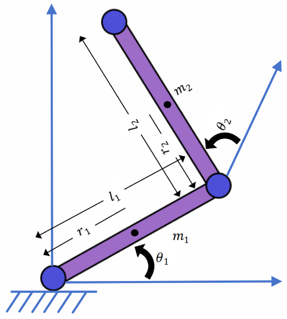
2.1. Manipulator Mathematical Model

This section presents an analysis of an n-jointed manipulator, with a description of its mechanical system’s dynamic performance based on the following Euler–Lagrange system:

$$M\left(\theta \right)\ddot{\theta }+C(\theta ,\dot{\theta })\dot{\theta }+G\left(\theta \right)+F\left(\dot{\theta }\right)+{\tau }_d=\tau$$

(1)

where $M\left(\theta \right)\in {\mathcal{R}}^{n\times n}$ denotes the symmetric positive definite inertia matrix, $C(\theta ,\dot{\theta })\in {\mathcal{R}}^n$ denotes the centripetal Coriolis matrix, $G\left(\theta \right)\in {\mathcal{R}}^n$ represents the gravity vector, $F\left(\dot{\theta }\right)\in {\mathcal{R}}^n$ represents the friction torque, ${\tau }_d\in {\mathcal{R}}^n$ denotes the disturbances, $\tau \in {\mathcal{R}}^n$ is the torque control vector, and $\theta \in {\mathcal{R}}^n,\dot{\theta }\in {\mathcal{R}}^n,\ddot{\theta }\in {\mathcal{R}}^n$ denote the rotation angle, velocity, and acceleration vectors, respectively. A schematic representation of a two-degree-of-freedom manipulator is presented in Figure 1.

Define $\theta =x_1\in {\mathcal{R}}^n,\dot{\theta }=x_2\in {\mathcal{R}}^n$; then, (1) can be rewritten as the following state space expression:

$$\left\{\begin{array}{c}{\dot{x}}_1=x_2\hfill \\ {\dot{x}}_2=\mathcal{F}+u+\mathcal{D}\hfill \\ y=x_1\hfill \end{array}\right.$$

(2)

where $\mathcal{F}=-M^{-1}\left(\theta \right)\left[C(\theta ,\dot{\theta })\dot{\theta }+G\left(\theta \right)+F\left(\dot{\theta }\right)\right]$, $u=M^{-1}\left(\theta \right)\tau$, $\mathcal{D}=-M^{-1}\left(\theta \right){\tau }_d$.

The objective of this paper is to design a prescribed performance anti-disturbance tracking controller for a hydraulic manipulator system with prescribed-time convergence. The system states do not violate the full-state constraints, and all signals are bounded in the presence of disturbances. Furthermore, the system state $x_1$ is capable of tracking the desired reference trajectory $x_d$, and neither the transient nor the steady-state performance violates the prescribed performance bounds. To achieve the control objective, the following assumptions are introduced.

Assumption A1. 

The reference trajectory $x_d$ and its derivatives ${\dot{x}}_d$ are known and bounded.

2.2. Prescribed-Time Control

Define a time-varying scaling function as

$$\sigma \left(t\right)=\left\{\begin{array}{c}{\displaystyle \frac{{\mathcal{T}}^m}{{(\mathcal{T}-t)}^m}},t\in [0,\mathcal{T})\hfill \\ 1,t\in [\mathcal{T},\infty )\hfill \end{array}\right.$$

(3)

and its derivatives is

$$\dot{\sigma }\left(t\right)=\left\{\begin{array}{c}{\displaystyle \frac{m{\mathcal{T}}^m}{{(\mathcal{T}-t)}^{m+1}}},t\in [0,\mathcal{T})\hfill \\ 0,t\in [\mathcal{T},\infty )\hfill \end{array}\right.$$

(4)

where m is the positive parameter of the function to be selected, and $\mathcal{T}>0$ represents a predetermined convergence time.

Definition 1 

([20]). Considering the following system

$$\dot{\mathcal{X}}\left(t\right)=f(t,\mathcal{X}\left(t\right)),\mathcal{X}\left(0\right)={\mathcal{X}}_0$$

(5)

where $\mathcal{X}\left(t\right)$ is the system state, f is a locally bounded function. If there exists a continuously differentiable function $V\left(\mathcal{X}\right(t),t)$, with a domain Δ such that

$$V(0,t)=0andV\left(\mathcal{X}\right(t),t)>0in\Delta -\left\{0\right\},$$

$$\dot{V}\le -kV-c{\displaystyle \frac{\dot{\sigma }\left(t\right)}{\sigma \left(t\right)}}V+bin\Delta ,$$

where $k>0$ is the convergence rate coefficient, $c\ge 2$ adjusts the influence of $\sigma \left(t\right)$, and $b\ge 0$ is the final boundary of bounded convergence, then the origin of system (5) is prescribed-time stable with the prescribed time $\mathcal{T}$ in (3).

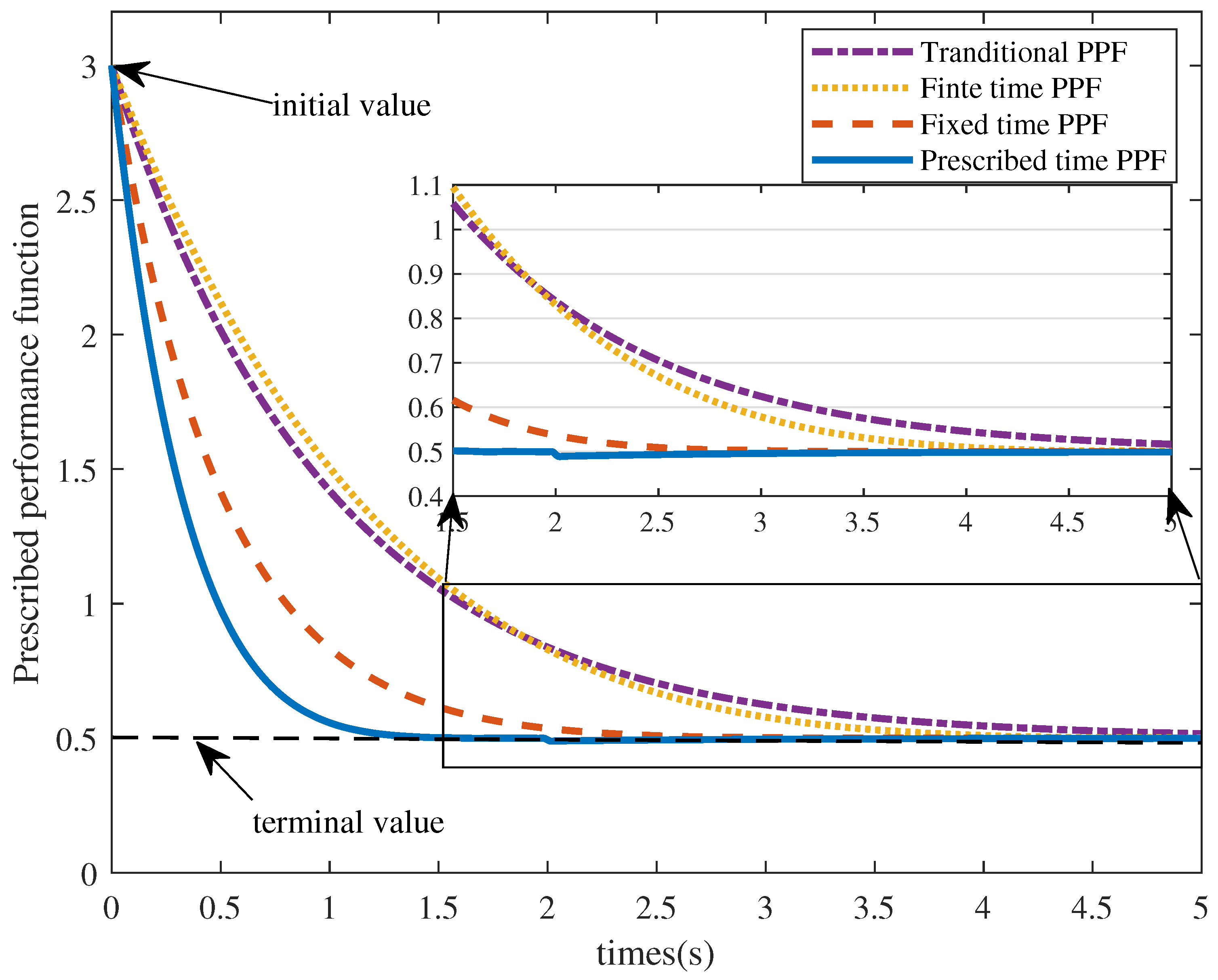
2.3. Prescribed-Time Prescribed Performance Control (PTPPC)

Define the tracking error $e_1=x_1-x_d$. In order to achieve the desired transient and steady-state performance, it is important to impose the following performance boundary constraints on the tracking error $e_1$:

$$-\eta \left(t\right)<e_1<\eta \left(t\right)$$

(6)

where $\eta \left(t\right)$ denotes a bounded and strictly monotonically decreasing smooth function, which is referred to as the prescribed performance function.

In order to obtain a deterministic convergence time, a novel prescribed-time prescribed performance function (PTPPF) is designed as follows:

$$\dot{\eta }\left(t\right)=-(k_{\eta }+c_{\eta }{\displaystyle \frac{\dot{\sigma }\left(t\right)}{\sigma \left(t\right)}})(\eta \left(t\right)-{\eta }_{\mathcal{T}})$$

(7)

where $k_{\eta }>0$ and $c_{\eta }\ge 2$ are positive constants to be designed, and ${\eta }_{\mathcal{T}}$ is the steady-state value of $\eta \left(t\right)$.

Theorem 1. 

Considering the PTPPF given by (7), the $\eta \left(t\right)$ can converge to the steady-state value ${\eta }_{\mathcal{T}}$ at the prescribed time $\mathcal{T}$. Moreover, when $t\ge \mathcal{T}$, $\eta \left(t\right)\equiv {\eta }_{\mathcal{T}}$ holds.

Proof of Theorem 1. 

Defining the error as $e_{\eta }=\eta -{\eta }_{\mathcal{T}}$, the derivative of $e_{\eta }$ can be obtained as follows:

$${\dot{e}}_{\eta }=-(k_{\eta }+c_{\eta }{\displaystyle \frac{\dot{\sigma }\left(t\right)}{\sigma \left(t\right)}})e_{\eta }$$

(8)

It can be obtained from Definition 1 that $e_{\eta }$ can converge to zero at the prescribed time $\mathcal{T}$. Thus, the proposed PTPPF $\eta$ can converge to ${\eta }_{\mathcal{T}}$ at the prescribed time $\mathcal{T}$. Theorem 1 is proven. □

Assumption A2. 

The initial error states satisfy our proposed error constraint $-\eta \left(0\right)<e_1\left(0\right)<\eta \left(0\right)$.

Remark 1. 

In contrast to the traditional prescribed performance function (PPF) described in [14], the finite-time PPF presented in [21], and the fixed-time PPF outlined in [19], the convergence time of the PTPPF, as devised in this paper, is not contingent on the initial conditions and design parameters of the system. Instead, it can be predetermined. A comparison plot of several PPF is given in Figure 2.

2.4. Prescribed-Time ESO (PTESO)

This subsection is dedicated to the PTESO design for the estimation of the total disturbance in system (2).

Define $x_3=\mathcal{F}+\mathcal{D}=\mathcal{H}$; then, we can obtain the extended state space expression

$$\left\{\begin{array}{c}{\dot{x}}_1=x_2\hfill \\ {\dot{x}}_2=x_3+u\hfill \\ {\dot{x}}_3=\dot{\mathcal{H}}\hfill \end{array}\right.$$

(9)

Assumption A3. 

$\dot{\mathcal{H}}$ is bounded, smooth, and continuous, i.e., $\dot{\mathcal{H}}\le H$, where H is a positive constant.

Remark 2. 

Assumption 3 is fundamental in constructing an ESO. It is based on the principle that the continuity and boundedness of $\dot{\mathcal{H}}$ can be obtained from the continuity and boundedness of $\mathcal{F}$ and $\mathcal{D}$.

In order to accurately estimate the total disturbance in the system within a prescribed time, a PTESO for system (9) is designed as follows:

$$\left\{\begin{array}{c}{\dot{z}}_1=z_2+\mathcal{P}\mathcal{W}\left(t\right){\mathcal{G}}_1(x_1-z_1)+(1-\mathcal{P})k_1{\mathcal{K}}^{1/3}si{g}^{2/3}(x_1-z_1)\hfill \\ {\dot{z}}_2=z_3+u+\mathcal{P}{\mathcal{W}}^2\left(t\right){\mathcal{G}}_2(x_1-z_1)+(1-\mathcal{P})k_2{\mathcal{K}}^{2/3}si{g}^{1/3}(x_1-z_1)\hfill \\ {\dot{z}}_3=\mathcal{P}{\mathcal{W}}^3\left(t\right){\mathcal{G}}_3(x_1-z_1)+(1-\mathcal{P})k_3\mathcal{K}si{g}^0(x_1-z_1)\hfill \end{array}\right.$$

(10)

where $\mathcal{W}\left(t\right)=cs{c}^2({\displaystyle \frac{\pi }{2}}-{\displaystyle \frac{\pi t}{2t_F}}),t\in [0,t_F)$, and $t_F$ is the prescribed convergence time for the PTESO; $\mathcal{K}$ is a Lipschitz constant to be designed, which satisfies $\mathcal{K}\ge H$; $k_{1,2,3}$ are the parameters to be designed, which satisfy $k_3>\mathcal{K},k_1=3.34k_3^{1/3},k_2=5.3k_3^{2/3}$; and $\mathcal{P}$ is the time-switching function of the PTESO, which satisfies

$$\mathcal{P}=\left\{\begin{array}{c}1,t\in [0,t_F)\hfill \\ 0,t\in [t_F,+\infty )\hfill \end{array}\right.$$

(11)

From (9) and (10), we can obtain the following observation error system:

$$\left\{\begin{array}{c}{\dot{\varphi }}_1={\varphi }_2-\mathcal{P}\mathcal{W}\left(t\right){\mathcal{G}}_1\left({\varphi }_1\right)-(1-\mathcal{P})k_1{\mathcal{K}}^{1/3}si{g}^{2/3}\left({\varphi }_1\right)\hfill \\ {\dot{\varphi }}_2={\varphi }_3-\mathcal{P}{\mathcal{W}}^2\left(t\right){\mathcal{G}}_2\left({\varphi }_1\right)-(1-\mathcal{P})k_2{\mathcal{K}}^{2/3}si{g}^{1/3}\left({\varphi }_1\right)\hfill \\ {\dot{\varphi }}_3=\dot{\mathcal{H}}-\mathcal{P}{\mathcal{W}}^3\left(t\right){\mathcal{G}}_3\left({\varphi }_1\right)+(1-\mathcal{P})k_3\mathcal{K}si{g}^0\left({\varphi }_1\right)\hfill \end{array}\right.$$

(12)

where ${\varphi }_1=x_1-z_1,{\varphi }_2=x_2-z_2,,{\varphi }_3=x_3-z_3$.

Lemma 1 

([22]). For system (9) with the designed PTESO (10), the observation error system (10) can achieve convergence within the prescribed time $t_F$, and they will be maintained at the origin within the time interval $t\in [t_F,+\infty )$.

Lemma 2 

([23]). For any positive constant M, any $N\in \mathcal{R}$ satisfies $\left|N\right|<M$. Then, we have ${\displaystyle \frac{N^2}{M^2-N^2}}>log{\displaystyle \frac{M^2}{M^2-N^2}}$, where $log(·)$ denotes the natural logarithm.

3. Main Results

This section presents the design of a multiple-constraint anti-disturbance tracking controller based on prescribed time for a hydraulic manipulator system. Based on the theory of prescribed-time convergence, a PTESO, a PTPPC, and a prescribed-time tracking controller are designed, respectively. The design of these components allows for the realization of preset time convergence in the system, while simultaneously ensuring that the constraints on the steady-state and transient performance of the system, the anti-disturbance performance of the system, and the full-state constraints are all met.

3.1. Control Design

In order to achieve the aforementioned control objective, we define ${\xi }_1={\displaystyle \frac{e_1}{\eta \left(t\right)}}$ and ${\xi }_2=x_2-{\alpha }_1$, where ${\alpha }_1$ is the virtual controller to be designed. The following two backstepping-based steps will be employed in order to construct and analyze the system’s controller.

Step 1. The derivation of the tracking error $e_1$ can be obtained as

$${\dot{e}}_1={\dot{x}}_1-{\dot{x}}_d$$

(13)

In order to achieve the desired state constraints, we have opted to combine BLF and PPC by defining a positive definite BLF as follows:

$$V_1={\displaystyle \frac{1}{2}}log{\displaystyle \frac{{\eta }^2\left(t\right)}{{\eta }^2\left(t\right)-e_1^2\left(t\right)}}={\displaystyle \frac{1}{2}}log{\displaystyle \frac{1}{1-{\xi }_1^2\left(t\right)}}$$

(14)

Differentiating $V_1$, substituting (13) into it yields

$$\begin{array}{cc}\hfill {\dot{V}}_1& ={\displaystyle \frac{{\xi }_1{\eta }^{-1}}{1-{\xi }_1^2}}({\dot{e}}_1-\dot{\eta }{\xi }_1)\hfill \\ \hfill & ={\displaystyle \frac{{\xi }_1{\eta }^{-1}}{1-{\xi }_1^2}}(x_2-{\dot{x}}_d-\dot{\eta }{\xi }_1)\hfill \\ \hfill & ={\displaystyle \frac{{\xi }_1{\eta }^{-1}}{1-{\xi }_1^2}}({\xi }_2+{\alpha }_1-{\dot{x}}_d-\dot{\eta }{\xi }_1)\hfill \end{array}$$

(15)

The virtual controller ${\alpha }_1$ is designed to be

$${\alpha }_1=-(k_{\alpha }+c_{\alpha }{\displaystyle \frac{\dot{\sigma }\left(t\right)}{\sigma \left(t\right)}}){\xi }_1+{\dot{x}}_d+\dot{\eta }{\xi }_1$$

(16)

where $k_{\alpha }>0$ and $c_{\alpha }\ge 2$ are positive constants to be designed.

Then, from (14) and (15), the dynamic $V_1$ becomes

$$\begin{array}{cc}\hfill {\dot{V}}_1& ={\displaystyle \frac{{\xi }_1{\eta }^{-1}}{1-{\xi }_1^2}}\left({\xi }_2-(k_{\alpha }+c_{\alpha }{\displaystyle \frac{\dot{\sigma }\left(t\right)}{\sigma \left(t\right)}}){\xi }_1\right)\hfill \\ \hfill & =-(k_{\alpha }+c_{\alpha }{\displaystyle \frac{\dot{\sigma }\left(t\right)}{\sigma \left(t\right)}}){\eta }^{-1}{\displaystyle \frac{{\xi }_1^2}{1-{\xi }_1^2}}+{\displaystyle \frac{{\xi }_1{\xi }_2{\eta }^{-1}}{1-{\xi }_1^2}}\hfill \end{array}$$

(17)

Step 2. The derivation of ${\xi }_2$ can be obtained as

$${\dot{\xi }}_2={\dot{x}}_2-{\dot{\alpha }}_1=\mathcal{F}+u+\mathcal{D}-{\dot{\alpha }}_1=x_3+u-{\dot{\alpha }}_1$$

(18)

Since the derivative of ${\alpha }_1$ cannot be obtained directly, the following linear tracking differentiator (LTD) is employed to approximate this variable:

$${\ddot{\widehat{\alpha }}}_1=-2r_1{\dot{\widehat{\alpha }}}_1-r_1^2\left({\widehat{\alpha }}_1-{\alpha }_1\right)$$

(19)

where $r_1$ is a positive parameter to be chosen, and ${\dot{\widehat{\alpha }}}_1$ is the estimation value of ${\dot{\alpha }}_1$.

Define the following positive definite BLF:

$$V_2={\displaystyle \frac{1}{2}}log{\displaystyle \frac{L_2^2}{L_2^2-{\xi }_2^2\left(t\right)}}$$

(20)

where $L_2>0$ is a design parameter.

Differentiating (20) and noting (18), we have

$$\begin{array}{cc}\hfill {\dot{V}}_2& ={\displaystyle \frac{{\xi }_2{\dot{\xi }}_2}{L_2^2-{\xi }_2^2\left(t\right)}}+{\dot{V}}_1\hfill \\ \hfill & ={\displaystyle \frac{{\xi }_2}{L_2^2-{\xi }_2^2\left(t\right)}}(x_3+u-{\dot{\alpha }}_1)+{\dot{V}}_1\hfill \end{array}$$

(21)

The controller u is designed to be

$$u=-(k_u+c_u{\displaystyle \frac{\dot{\sigma }\left(t\right)}{\sigma \left(t\right)}}){\xi }_2-z_3+{\dot{\widehat{\alpha }}}_1-{\displaystyle \frac{{\xi }_1{\eta }^{-1}(L_2^2-{\xi }_2^2\left(t\right))}{1-{\xi }_1^2}}-{\xi }_2(L_2^2-{\xi }_2^2\left(t\right))$$

(22)

3.2. Stability Analysis

Theorem 2. 

Consider the system (1), PTESO (10), virtual control law (16), and prescribed-time based anti-disturbance controller (21) subject to system uncertainties. Under Assumptions 1–3, for any initial state, the prescribed-time convergence of the distributed hydraulic manipulator system can be guaranteed. Moreover, the convergence time is $\mathcal{T}$, and the tracking error $e_1$ can remain within the performance specification (6).

Proof of Theorem 2. 

Substituting (22) into (21), we have

$$\begin{array}{cc}\hfill {\dot{V}}_2=& {\displaystyle \frac{{\xi }_2}{L_2^2-{\xi }_2^2\left(t\right)}}\left(\right(x_3-(k_u+c_u{\displaystyle \frac{\dot{\sigma }\left(t\right)}{\sigma \left(t\right)}}){\xi }_2-z_3+{\dot{\widehat{\alpha }}}_1-{\displaystyle \frac{{\xi }_1{\eta }^{-1}(L_2^2-{\xi }_2^2\left(t\right))}{1-{\xi }_1^2}}\hfill \\ \hfill & -{\xi }_2(L_2^2-{\xi }_2^2\left(t\right))-{\dot{\alpha }}_1\left)\right)+{\dot{V}}_1\hfill \\ \hfill =& -(k_{\alpha }+c_{\alpha }{\displaystyle \frac{\dot{\sigma }\left(t\right)}{\sigma \left(t\right)}}){\eta }^{-1}{\displaystyle \frac{{\xi }_1^2}{1-{\xi }_1^2\left(t\right)}}-(k_u+c_u{\displaystyle \frac{\dot{\sigma }\left(t\right)}{\sigma \left(t\right)}}){\displaystyle \frac{{\xi }_2^2}{L_2^2-{\xi }_2^2\left(t\right)}}+{\displaystyle \frac{{\xi }_2(x_3-z_3)}{L_2^2-{\xi }_2^2\left(t\right)}}\hfill \\ \hfill & +{\displaystyle \frac{{\xi }_2({\dot{\widehat{\alpha }}}_1-{\dot{\alpha }}_1)}{L_2^2-{\xi }_2^2\left(t\right)}}-{\xi }_2^2\hfill \end{array}$$

(23)

With the help of Young’s inequality, one has

$$\begin{array}{cc}\hfill {\dot{V}}_2\le & -(k_{\alpha }+c_{\alpha }{\displaystyle \frac{\dot{\sigma }\left(t\right)}{\sigma \left(t\right)}}){\eta }^{-1}{\displaystyle \frac{{\xi }_1^2}{1-{\xi }_1^2\left(t\right)}}-(k_u+c_u{\displaystyle \frac{\dot{\sigma }\left(t\right)}{\sigma \left(t\right)}}){\displaystyle \frac{{\xi }_2^2}{L_2^2-{\xi }_2^2\left(t\right)}}\hfill \\ \hfill & +{\displaystyle \frac{{(x_3-z_3)}^2}{{(L_2^2-{\xi }_2^2\left(t\right))}^2}}+{\displaystyle \frac{{({\dot{\widehat{\alpha }}}_1-{\dot{\alpha }}_1)}^2}{{(L_2^2-{\xi }_2^2\left(t\right))}^2}}\hfill \end{array}$$

(24)

According to Lemma 2, $log{\displaystyle \frac{1}{1-{\xi }_1^2}}<{\displaystyle \frac{{\xi }_1^2}{1-{\xi }_1^2}}$ and $log{\displaystyle \frac{1}{L_2^2-{\xi }_2^2}}<{\displaystyle \frac{{\xi }_2^2}{L_2^2-{\xi }_2^2}}$, and

$$\begin{array}{cc}\hfill {\dot{V}}_2\le & -(k_{\alpha }+c_{\alpha }{\displaystyle \frac{\dot{\sigma }\left(t\right)}{\sigma \left(t\right)}}){\eta }^{-1}log{\displaystyle \frac{1}{1-{\xi }_1^2}}-(k_u+c_u{\displaystyle \frac{\dot{\sigma }\left(t\right)}{\sigma \left(t\right)}})log{\displaystyle \frac{1}{L_2^2-{\xi }_2^2}}\hfill \end{array}$$

$$\begin{array}{cc}\hfill & +{\displaystyle \frac{{(x_3-z_3)}^2}{{(L_2^2-{\xi }_2^2\left(t\right))}^2}}+{\displaystyle \frac{{({\dot{\widehat{\alpha }}}_1-{\dot{\alpha }}_1)}^2}{{(L_2^2-{\xi }_2^2\left(t\right))}^2}}\hfill \end{array}$$

(25)

$$\begin{array}{cc}\hfill \le & -(k_M+c_M{\displaystyle \frac{\dot{\sigma }\left(t\right)}{\sigma \left(t\right)}})V_2+b_M\hfill \end{array}$$

(26)

where $k_M=min\{k_{\alpha }{\eta }^{-1},k_u\}$, $c_M=min\{c_{\alpha }{\eta }^{-1},c_u\}$, $b_M={\displaystyle \frac{{(x_3-z_3)}^2}{{(L_2^2-{\xi }_2^2\left(t\right))}^2}}+{\displaystyle \frac{{({\dot{\widehat{\alpha }}}_1-{\dot{\alpha }}_1)}^2}{{(L_2^2-{\xi }_2^2\left(t\right))}^2}}$.

According to Definition 1, the system is prescribed-time stable with the prescribed time $\mathcal{T}$ in (3). Theorem 2 is proven. □

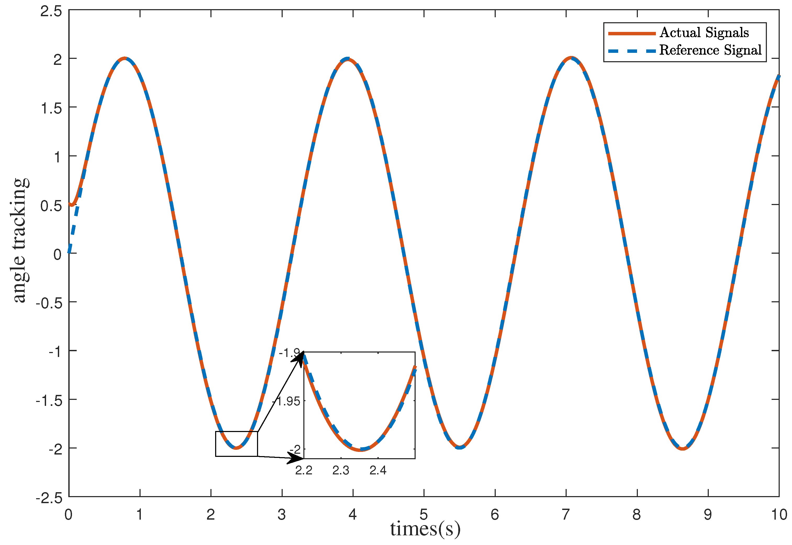
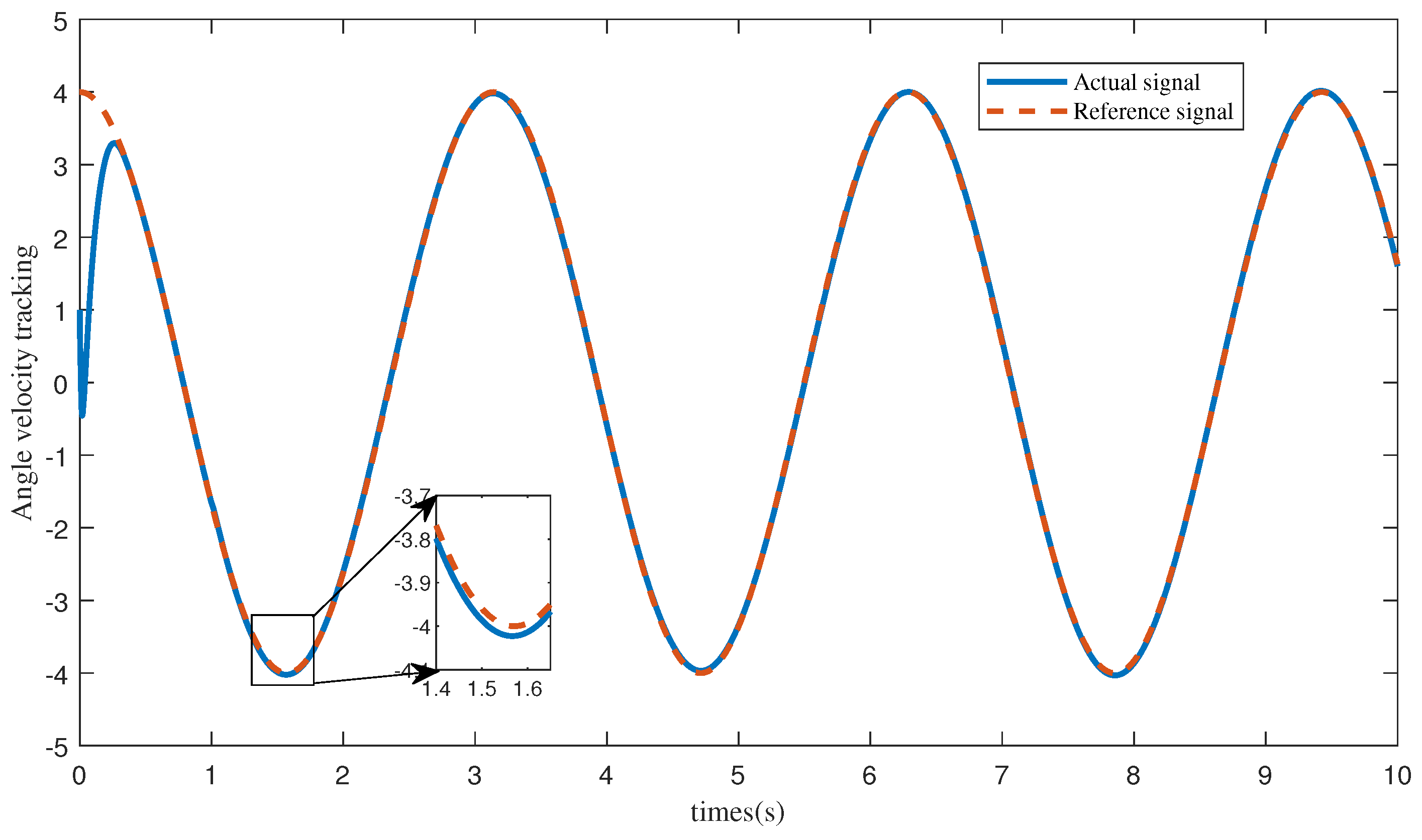
4. Numerical Simulation

In order to ascertain the efficacy of the devised prescribed-time prescribed performance anti-disturbance tracking controller, we consider a single force manipulator exhibiting the following dynamics:

$$I\ddot{\theta }+d\dot{\theta }+Mglcos\left(\theta \right)+{\tau }_d=\tau$$

(27)

where the detailed expressions are $I={\displaystyle \frac{4}{3}}M{l}^2$, $M=1$ kg, $l=0.25$ m, $d=2$ m. The objective of the simulation is to ensure that the system states $x_1$ and $x_2$ align with the desired reference signal $x_d=2sin\left(2t\right)$ and the virtual control ${\alpha }_1$, respectively, while adhering to the full-state constraints. The initial conditions of the system state are presented as follows: $x_1\left(0\right)=0.5,x_2\left(0\right)=1$. The initial values of all states of the PTESO and LTD are set to zero, i.e., $z_1\left(0\right)=0,z_2\left(0\right)=0,z_3\left(0\right)=0,\widehat{\alpha }=0,\dot{\widehat{\alpha }}\left(0\right)=0$. The parameters in the time-varying scaling function (3), PTPPF (7), PTESO (10), virtual controller (16), and controller (22) are selected as the following: $\mathcal{T}=1$ s, $m=4,k_{\eta }=1,c_{\eta }=2,{\eta }_{\mathcal{T}}=0.4,{\mathcal{G}}_1=6,$${\mathcal{G}}_2=8,{\mathcal{G}}_3=2,\mathcal{K}=4,k_3=5,k_{\alpha }=1,c_{\alpha }=2,k_u=1,c_u=2,L_2=10$.

The simulation results for the prescribed-time multiple-constraint anti-disturbance tracking control algorithm are presented in Figure 3, Figure 4, Figure 5, Figure 6, Figure 7 and Figure 8.

Figure 3 illustrates the evolution of the actual and desired angles over time. The solid line represents the actual angle, while the dashed line depicts the desired angle. It can be observed that, at the outset, there is a considerable discrepancy between the actual and desired angles. However, after a brief interval (t = 0.2), the actual angle of the system exhibits rapid convergence towards the desired angle, accompanied by a gradual reduction in the error until it is nearly indistinguishable. The entire process is completed within the prescribed time (t = 1), indicating that the system displays remarkable responsiveness and is capable of accurately executing trajectory tracking.

Figure 4 illustrates the trend of the actual and desired angular velocities of the system. During the initial stage, the system’s angular velocity fluctuates, but it rapidly converges in a short period of time (t = 0.2) and subsequently stabilizes around the desired angular velocity value. As time progresses, the deviation of the actual angular velocity from the desired value decreases.

Figure 5 illustrates the tracking error over time and the range of performance boundaries within which the error falls. The curves demonstrate that the error is initially considerable but then decreases rapidly and ultimately remains within the prescribed performance boundaries. This indicates that the system is not only capable of achieving precise trajectory tracking within the specified time frame but also ensures that the tracking error is consistently below the defined constraints.

Figure 6 illustrates the estimation error of the PTESO for external disturbances. The curves demonstrate that the observation error is initially considerable and then decays rapidly with time, reaching a minimum at approximately t = 1 s. This indicates that the PTESO is capable of rapidly estimating and compensating for disturbances in the system, thereby enabling the system to achieve high-precision disturbance suppression within a prescribed time.

Figure 7 illustrates the evolution of the conversion error ${\xi }_1$ and the tracking error ${\xi }_2$ over time. The curves indicate that ${\xi }_1$ and ${\xi }_2$ are initially significant but rapidly converge to a small neighborhood around 0 at approximately time t = 1 s. This suggests that the system reaches a steady state within a preset time under the action of the designed controller, thereby effectively verifying the effectiveness of the designed controller. Figure 8 depicts the evolution of the virtual and real controllers over time.

5. Conclusions

This paper presents the design of a comprehensive tracking controller for a hydraulic manipulator system. The controller incorporates advanced control strategies, including prescribed-time convergence control, PPC, output constraint control based on the BLF, and anti-disturbance control based on the PTESO. The system stability of the proposed control scheme is rigorously demonstrated through the use of a Lyapunov function, which ensures the reliable convergence and performance of the controller. The effectiveness and robustness of the designed controller in realizing accurate trajectory tracking under multiple constraints and disturbances is further verified by numerical simulations. The control method proposed in this paper has the potential to be applied in the practical use of manipulators that require high-precision tracking and anti-disturbance capabilities. Further experimental validation and the extension of the framework to application scenarios in multi-DOF manipulators or highly dynamic, uncertain environments can be carried out in future research.

References

1. Zhang, C.; Guan, M.; Zhang, G. Signal generator based prescribed-time anti-disturbance containment control for multi-agent systems with an application to multiple manipulator system. In Proceedings of the 2024 International Conference on Advanced Control Systems and Automation Technologies (ACSAT), Nanjing, China, 15–17 November 2024. [Google Scholar]
2. Wang, W.; Chi, H.; Zhao, S.; Du, Z. A control method for hydraulic manipulators in automatic emulsion filling. Autom. Constr. 2018, 91, 92–99. [Google Scholar] [CrossRef]
3. Nurmi, J.; Mattila, J. Global energy-optimal redundancy resolution of hydraulic manipulators: Experimental results for a forestry manipulator. Energies 2017, 10, 647. [Google Scholar] [CrossRef]
4. Mattila, J.; Koivumäki, J.; Caldwell, D.G.; Semini, C. A survey on control of hydraulic robotic manipulators with projection to future trends. IEEE/ASME Trans. Mechatron. 2017, 22, 669–680. [Google Scholar]
5. Siwek, M.; Baranowski, L.; Ładyżyńska-Kozdraś, E. The Application and Optimisation of a Neural Network PID Controller for Trajectory Tracking Using UAVs. Sensors 2024, 24, 8072. [Google Scholar] [CrossRef]
6. Melo, A.G.; Andrade, F.A.; Guedes, I.P.; Carvalho, G.F.; Zachi, A.R.; Pinto, M.F. Fuzzy gain-scheduling PID for UAV position and altitude controllers. Sensors 2022, 22, 2173. [Google Scholar] [CrossRef]
7. Song, Y.; Wang, Y.; Holloway, J.; Krstic, M. Time-varying feedback for regulation of normal-form nonlinear systems in prescribed finite time. Automatica 2017, 83, 243–251. [Google Scholar] [CrossRef]
8. Hua, C.; Ning, P.; Li, K. Adaptive prescribed-time control for a class of uncertain nonlinear systems. IEEE Trans. Autom. Control 2021, 67, 6159–6166. [Google Scholar]
9. Wang, Y.; Song, Y.; Hill, D.J.; Krstic, M. Prescribed-time consensus and containment control of networked multiagent systems. IEEE Trans. Cybern. 2018, 49, 1138–1147. [Google Scholar]
10. Siwek, M. Consensus-Based Formation Control with Time Synchronization for a Decentralized Group of Mobile Robots. Sensors 2024, 24, 3717. [Google Scholar] [CrossRef]
11. Tee, K.P.; Ge, S.S.; Tay, E.H. Barrier Lyapunov functions for the control of output-constrained nonlinear systems. Automatica 2009, 45, 918–927. [Google Scholar]
12. Xie, Z.; Chen, X.; Wu, X. Fixed time control of free-flying space robotic manipulator with full state constraints: A barrier-Lyapunov-function term free approach. Nonlinear Dyn. 2024, 112, 1883–1915. [Google Scholar] [CrossRef]
13. Cruz-Ortiz, D.; Chairez, I.; Poznyak, A. Non-singular terminal sliding-mode control for a manipulator robot using a barrier Lyapunov function. ISA Trans. 2022, 121, 268–283. [Google Scholar] [CrossRef] [PubMed]
14. Bechlioulis, C.P.; Rovithakis, G.A. Robust adaptive control of feedback linearizable MIMO nonlinear systems with prescribed performance. IEEE Trans. Autom. Control 2008, 53, 2090–2099. [Google Scholar] [CrossRef]
15. Deng, W.; Zhou, H.; Zhou, J.; Yao, J. Neural network-based adaptive asymptotic prescribed performance tracking control of hydraulic manipulators. IEEE Trans. Syst. Man Cybern. Syst. 2022, 53, 285–295. [Google Scholar] [CrossRef]
16. Guo, Q.; Zhang, Y.; Celler, B.G.; Su, S.W. Neural adaptive backstepping control of a robotic manipulator with prescribed performance constraint. IEEE Trans. Neural Netw. Learn. Syst. 2018, 30, 3572–3583. [Google Scholar] [CrossRef]
17. Han, J. From PID to Active Disturbance Rejection Control. IEEE Trans. Ind. Electron. 2009, 56, 900–906. [Google Scholar] [CrossRef]
18. Zhang, X.; Shi, G. Dual extended state observer-based adaptive dynamic surface control for a hydraulic manipulator with actuator dynamics. Mech. Mach. Theory 2022, 169, 104647. [Google Scholar] [CrossRef]
19. Zhang, C.; Zhang, G.; Han, W.; Lv, X.; Shi, Z. Distributed fixed-time control for high-order multi-agent systems with FTESO and feasibility constraints. J. Frankl. Inst. 2024, 361, 107219. [Google Scholar] [CrossRef]
20. Song, Y.; Ye, H.; Lewis, F.L. Prescribed-time control and its latest developments. IEEE Trans. Syst. Man Cybern. Syst. 2023, 53, 4102–4116. [Google Scholar] [CrossRef]
21. Gao, S.; Liu, X.; Dimirovski, G.M. Finite-time prescribed performance control for spacecraft attitude tracking. IEEE/ASME Trans. Mechatron. 2021, 27, 3087–3098. [Google Scholar] [CrossRef]
22. Cui, L.; Jin, N. Prescribed-time ESO-based prescribed-time control and its application to partial IGC design. Nonlinear Dyn. 2021, 106, 491–508. [Google Scholar]
23. Zhao, Z.; He, W.; Ge, S.S. Adaptive neural network control of a fully actuated marine surface vessel with multiple output constraints. IEEE Trans. Control Syst. Technol. 2013, 22, 1536–1543. [Google Scholar]
Figure 1. Schematic diagram of two-DOF manipulator.
Actuators 14 00157 g001
Figure 2. A comparison of different prescribed performance functions.
Actuators 14 00157 g002
Figure 3. The trajectory of angle tracking over time.
Actuators 14 00157 g003
Figure 4. The trajectory of angle velocity tracking over time.
Actuators 14 00157 g004
Figure 5. The tracking errors e 1 along with the prescribed-time performance bounds η and η .
Actuators 14 00157 g005
Figure 6. The observation errors ϕ 1 , ϕ 2 , and ϕ 3 of the PTESO.
Actuators 14 00157 g006
Figure 7. (a) The transformed error ξ 1 . (b) The tracking error ξ 2 .
Actuators 14 00157 g007
Figure 8. (a) The virtual controller α 1 . (b) The controller u.
Actuators 14 00157 g008
Disclaimer/Publisher’s Note: The statements, opinions and data contained in all publications are solely those of the individual author(s) and contributor(s) and not of MDPI and/or the editor(s). MDPI and/or the editor(s) disclaim responsibility for any injury to people or property resulting from any ideas, methods, instructions or products referred to in the content.