Command-Filtered Yaw Stability Control of Vehicles with State Constraints

Abstract

Yaw stability control is crucial for ensuring the driving safety of intelligent vehicles. This paper proposes a state-constrained command-filtered control (CFC) approach for vehicle yaw stability. The proposed method employs a barrier Lyapunov function (BLF) to effectively constrain the vehicle’s sideslip angle and yaw rate, thereby enhancing system stability and safety. Meanwhile, a command-filtered control strategy is introduced to reduce computational complexity, and an error compensation mechanism is incorporated to mitigate the adverse effects of filter-induced errors on system performance. To validate the effectiveness and robustness of the proposed method, simulations are conducted under different road adhesion conditions and driving speeds. The results demonstrate that the proposed control approach effectively suppresses both understeer and oversteer phenomena, significantly improving vehicle handling stability. This study provides theoretical support and practical insights for the engineering application of yaw stability control in intelligent vehicles.

1. Introduction

With the rapid advancement of intelligent vehicle technology, the role of active safety control in the overall vehicle system architecture has become increasingly prominent [1], playing a crucial role in enhancing driving safety. During vehicle steering, complex and dynamic driving conditions may cause the vehicle to deviate from the driver’s intended trajectory, leading to understeer or oversteer, which can further result in lateral instability, such as oversteer-induced skidding or understeer-induced plowing. These instability phenomena not only reduce vehicle handling stability but also make it difficult for drivers to maintain effective control, potentially leading to severe traffic accidents [2]. Consequently, improving vehicle handling stability based on active safety control technologies has become one of the core topics in the research field of intelligent vehicle safety. Direct yaw moment control (DYC) is an efficient active safety system that regulates tire longitudinal forces by applying differential driving or braking torques to individual wheels. This approach generates additional yaw moments to control the vehicle’s sideslip angle and yaw rate, thereby correcting its yaw motion state. DYC can effectively suppress lateral instability under extreme conditions such as emergency steering, significantly improving both vehicle stability and active safety performance [3].

Currently, DYC methods primarily include fuzzy control [4,5,6], sliding mode control [7,8,9], robust control [10,11], and model predictive control (MPC) [12,13,14,15,16]. Backstepping control and its enhanced methodologies have been widely recognized as effective nonlinear control strategies in industrial applications [17]. However, compared to the aforementioned commonly used methods, their application in direct yaw control (DYC) remains relatively limited. For instance, Reference [18] proposed a composite adaptive backstepping robust tracking controller to enhance the lateral stability of electric vehicles (EVs) under parameter uncertainties and external disturbances. A nonlinear three-degree-of-freedom model was employed to characterize the vehicle’s lateral and roll dynamics. By integrating adaptive backstepping with dynamic surface control, the proposed controller ensures that the sideslip angle and yaw rate converge to their desired reference values, with asymptotic stability rigorously established using Lyapunov theory. CarSim-Simulink simulations conducted under single-lane-change and J-turn maneuvers validate its effectiveness, demonstrating superior robustness and tracking performance compared to conventional approaches. Reference [19] developed a sideslip angle control system for an e-4WD vehicle equipped with front in-wheel motors and a rear active differential to enhance cornering performance. A backstepping controller was designed to generate the desired yaw moment based on a bicycle model, incorporating feedforward terms to improve responsiveness. Torque distribution, implemented via a daisy-chaining strategy, optimally coordinates the actuation of the front in-wheel motors and rear axle. CarSim simulations confirm that the proposed approach achieves superior cornering performance compared to conventional feedback controllers. Reference [20] proposed a robust constrained control scheme for DYC systems with sideslip angle constraints. Utilizing a two-degree-of-freedom vehicle model and tangent barrier Lyapunov functions (BLFs-Tan), the designed nonlinear controller ensures precise reference trajectory tracking while preventing sideslip angle violations and vehicle instability. The simulation results validate the scheme’s effectiveness in maintaining constraint adherence and enhancing stability under dynamic conditions, demonstrating superior robustness compared to conventional methods.

Although the state-constrained control method based on the barrier Lyapunov function (BLF) [21], as proposed in Reference [20], explicitly accounts for state constraints in control law design, ensuring system stability while enhancing control flexibility, it inevitably involves the differentiation of virtual control laws during the controller design process, leading to the issue of computational explosion. To address this problem, command-filtered control (CFC) [22] introduces an error compensation mechanism to mitigate the accumulation of filtering errors. Additionally, CFC employs a command-filtered strategy to smooth control inputs, effectively suppressing high-frequency chattering and noise interference in the control process, thereby improving the stability and robustness of the control system. For example, Reference [23] proposed a predefined-time control approach for nonlinear systems with preassigned performance metrics and state constraints. The approach combined barrier Lyapunov functions, recursive command-filtered backstepping, and predefined-time convergence indicators, thereby simplifying stability analysis. Reference [24] proposed a command-filtered backstepping quantized consensus control approach for time-varying full-state-constrained nonlinear multiagent systems. The approach employed a novel TVSC-USDE for accurate dynamic estimation, integral barrier Lyapunov functions to mitigate feasibility conservatism, and error compensation to manage the explosion of complexity. It ensured consensus tracking with low communication rates and minimal tracking errors. Reference [25] investigated an adaptive event-triggered control strategy for switched nonlinear systems with full-state time-varying constraints. The strategy integrated command-filtered backstepping, dynamic surface control, and RBFNN-based approximation to ensure SGUUB stability under arbitrary switching, while guaranteeing constraint satisfaction and Zeno-free execution.

In summary, this paper integrates the advantages of the asymmetric barrier Lyapunov function (ABLF) and CFC to address the yaw stability control problem of intelligent vehicles with full-state constraints. The proposed control algorithm explicitly incorporates constraint boundaries for the vehicle’s sideslip angle and yaw rate, and a yaw stability command-filtered control strategy based on ABLF is developed. The effectiveness of the proposed control scheme is validated through simulation experiments, providing theoretical support and technical reference for practical applications in intelligent vehicles. The proposed control method offers the following advantages:

①

By constructing the controller based on the ABLF, the proposed approach ensures that the sideslip angle and yaw rate remain within reasonable bounds, effectively imposing both symmetric and asymmetric constraints on state variables, thereby enhancing the adaptability and flexibility of the control algorithm.

②

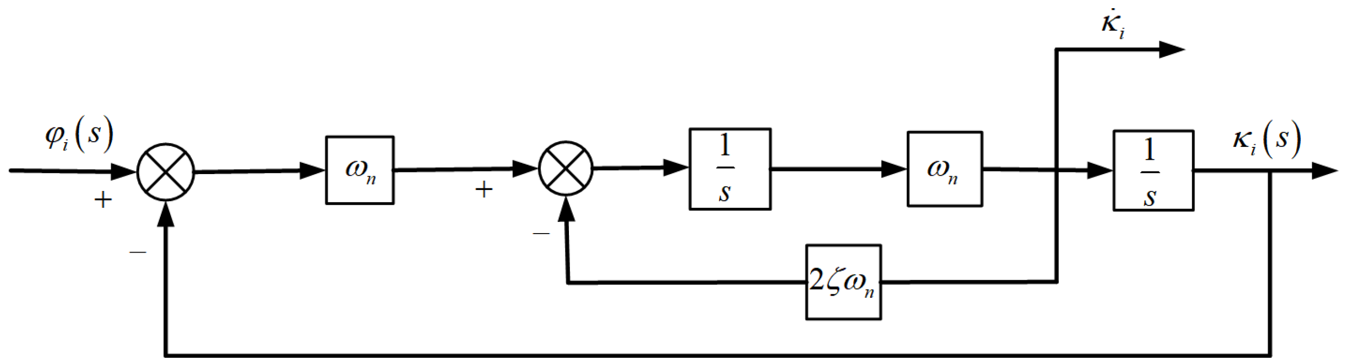
The adoption of the second-order command-filtered method enables the computation of filtered virtual control signals and their derivatives through a command filter, avoiding the need for direct differentiation of virtual control inputs and effectively mitigating the potential issue of computational explosion in control law derivation.

③

A filtering error compensation mechanism is incorporated to reduce errors introduced by the command filter, further improving control accuracy. The proposed control scheme guarantees that the state error of the closed-loop system ultimately converges to a compact set, thereby enhancing the robustness and precision of yaw stability control.

2. Coupled Dynamic Model of Intelligent Vehicles and Problem Formulation

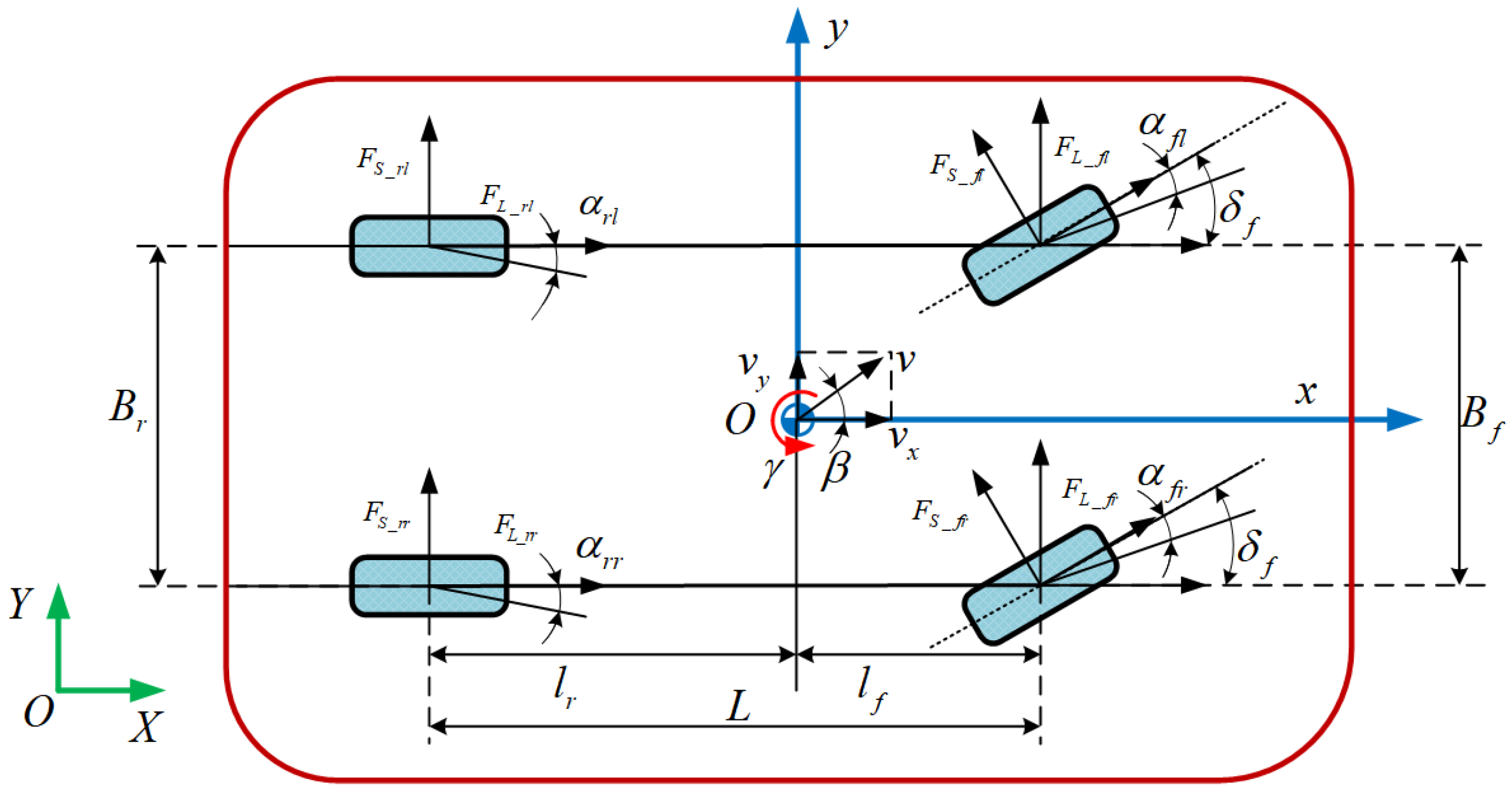
2.1. Coupled Dynamics Model of Intelligent Vehicles

This study investigates the characteristics of intelligent vehicles during steering maneuvers. To simplify computational complexity, vehicle motion in other degrees of freedom is neglected, and it is assumed that the steering angles of both front wheels are identical. A nonlinear vehicle dynamics model is established, incorporating lateral, yaw, and longitudinal dynamics, as well as the rotational dynamics of all four wheels. The standard vehicle coordinate system is adopted, establishing the Oxyz coordinate system, where O represents the origin at the vehicle’s center of mass. The x-axis points in the forward driving direction, the y-axis points in the positive lateral (steering) direction, and the z-axis extends vertically from the center of mass O, perpendicular to the Oxyz plane.

As shown in Figure 1, the motion equations of the intelligent vehicle are derived based on Newtonian mechanics, as follows [26].

Longitudinal motion dynamics along the x-axis:

$$\begin{array}{l}m({\dot{\nu }}_x-{\nu }_y\gamma )={\displaystyle \sum F_{X\_i}}\\ =(F_{L\_fl}+F_{L\_fr})\cos {\delta }_f-(F_{S\_fl}+F_{S\_fr})\sin {\delta }_f+F_{L\_rl}+F_{L\_rr}\end{array}$$

(1)

${\displaystyle \sum F_{X\_i}}$ represents the total sum of the longitudinal force components acting along the x-axis on the wheels.

Lateral motion dynamics along the y-axis:

$$\begin{array}{l}m({\dot{\nu }}_y+{\nu }_x\gamma )={\displaystyle \sum F_{Y\_i}}\\ =(F_{L\_fl}+F_{L\_fr})\sin {\delta }_f+(F_{S\_fl}+F_{S\_fr})\cos {\delta }_f+F_{S\_rl}+F_{S\_rr}\end{array}$$

(2)

${\displaystyle \sum F_{Y\_i}}$ represents the total sum of the lateral force components of the wheels along the y-axis.

Lateral motion dynamics along the z-axis:

$$\begin{array}{l}{I}_z\dot{\gamma }={\displaystyle \sum M_{Z\_i}}\\ ={\displaystyle \frac{B_f}{2}}\left[(F_{L\_fr}-F_{L\_fl})\cos {\delta }_f+(F_{S\_fl}-F_{S\_fr})\sin {\delta }_f\right]+{\displaystyle \frac{B_r}{2}}(F_{L\_rr}-F_{L\_rl})\\ +l_f\left[(F_{L\_fl}+F_{L\_fr})\sin {\delta }_f+l_f(F_{S\_fl}+F_{S\_fr})\cos {\delta }_f\right]-l_r(F_{S\_rl}+F_{S\_rr})\end{array}$$

(3)

where ${\displaystyle \sum M_{Z\_i}}$ is the total yaw moment, $l_f$ is the distance from the car’s center of mass to the front axle, and $l_r$ is the distance from the car’s center of mass to the rear axle; $L=l_f+l_r$ is the wheelbase; ${\delta }_f$ is the steering angle of the front wheels; $\gamma$ is the yaw rate; $v_x$ is the longitudinal (forward) speed; $v_y$ is the lateral speed; $B_f$ and $B_r$ represent the wheelbase of the front and rear axles, respectively; $F_{L\_i}\left(i=fl,\hspace{0.33em}fr,\hspace{0.33em}rl,\hspace{0.33em}rr\right)$ are the longitudinal force on the wheels; $F_{S\_i}\left(i=fl,\hspace{0.33em}fr,\hspace{0.33em}rl,\hspace{0.33em}rr\right)$ are the lateral force on the wheels; m is the total mass of the car; $I_z$ is the moment of inertia of the entire vehicle about the z-axis; $i=fl,\hspace{0.33em}fr,\hspace{0.33em}rl,\hspace{0.33em}rr$, respectively, represent the front left, front right, rear left, and rear right wheels of the car.

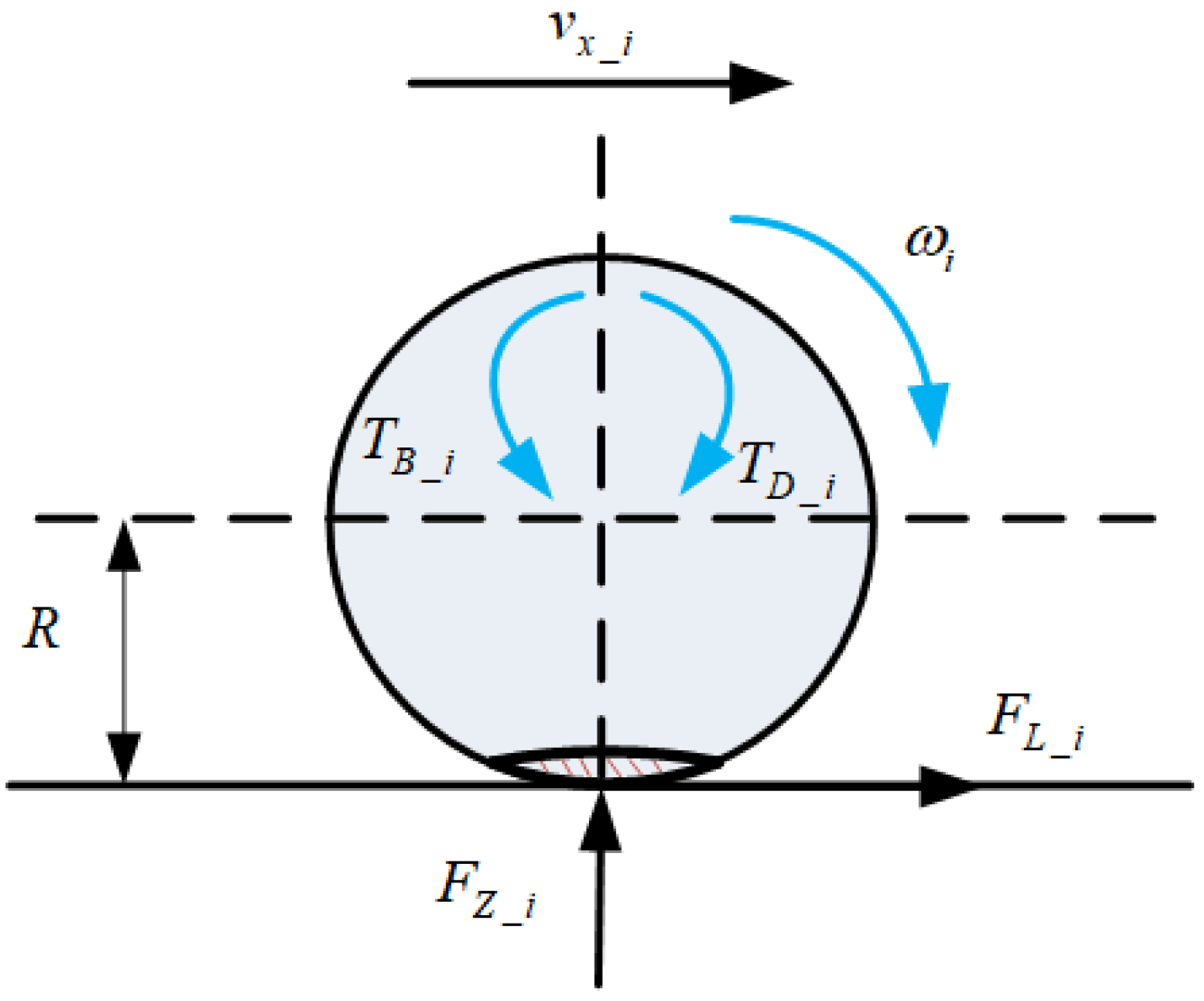
2.1.1. Rotational Dynamics Model of Each Wheel

During vehicle operation, the wheels are subjected to various forces, and their force model is illustrated in Figure 2.

Based on the forces acting on the wheel, we obtain the wheel’s rotational equation:

$$J_i{\dot{\omega }}_i=T_{D\_i}-T_{B\_i}-F_{L\_i}R$$

(4)

where ${\omega }_i$ represents the rotational angular velocity of each wheel, $T_{D\_i}$ denotes the driving torque of each wheel, $T_{B\_i}$ represents the braking torque of each wheel, $J_i$ is the rotational inertia of each wheel, and R is the rolling radius of the wheel.

2.1.2. Vertical Load of Each Wheel

$$\left\{\begin{array}{l}{F}_{Z\_fl}=mg{\displaystyle \frac{l_r}{2L}}-{\displaystyle \frac{m({\dot{\nu }}_x-{\nu }_y\gamma )h_{cg}}{2L}}-{\displaystyle \frac{m({\dot{\nu }}_y+{\nu }_x\gamma )l_r{h}_{cg}}{L{B}_f}}\\ F_{Z\_fr}=mg{\displaystyle \frac{l_r}{2L}}-{\displaystyle \frac{m({\dot{\nu }}_x-{\nu }_y\gamma )h_{cg}}{2L}}+{\displaystyle \frac{m({\dot{\nu }}_y+{\nu }_x\gamma )l_r{h}_{cg}}{L{B}_f}}\\ F_{Z\_rl}=mg{\displaystyle \frac{l_f}{2L}}+{\displaystyle \frac{m({\dot{\nu }}_x-{\nu }_y\gamma )h_{cg}}{2L}}-{\displaystyle \frac{m({\dot{\nu }}_y+{\nu }_x\gamma )l_f{h}_{cg}}{L{B}_r}}\\ F_{Z\_rr}=mg{\displaystyle \frac{l_f}{2L}}+{\displaystyle \frac{m({\dot{\nu }}_x-{\nu }_y\gamma )h_{cg}}{2L}}+{\displaystyle \frac{m({\dot{\nu }}_y+{\nu }_x\gamma )l_f{h}_{cg}}{L{B}_r}}\end{array}\right.$$

(5)

where $h_g$ represents the height of the center of gravity.

2.1.3. Tire Slip Angles of Each Wheel

$$\left\{\begin{array}{l}{\alpha }_{fl}=\arctan ({\displaystyle \frac{v_y+l_f\gamma }{v_x-\frac{B_f}{2}\gamma }})-{\delta }_f\\ {\alpha }_{fr}=\arctan ({\displaystyle \frac{v_y+l_f\gamma }{v_x+\frac{B_f}{2}\gamma }})-{\delta }_f\\ {\alpha }_{rl}=\arctan ({\displaystyle \frac{v_y-l_r\gamma }{v_x-\frac{B_r}{2}\gamma }})\\ {\alpha }_{rr}=\arctan ({\displaystyle \frac{v_y-l_r\gamma }{v_x+\frac{B_r}{2}\gamma }})\end{array}\right.$$

(6)

where ${\alpha }_i\left(i=fl,\hspace{0.33em}fr,\hspace{0.33em}rl,\hspace{0.33em}rr\right)$ is the slip angle of each wheel.

2.1.4. Longitudinal Velocities of Each Wheel

$$\left\{\begin{array}{l}{v}_{x\_fl}=(v_x-{\displaystyle \frac{B_f}{2}}\gamma )\cos {\delta }_f+(v_y+l_f\gamma )\sin {\delta }_f\\ v_{x\_fr}=(v_x+{\displaystyle \frac{B_f}{2}}\gamma )\cos {\delta }_f+(v_y+l_f\gamma )\sin {\delta }_f\\ v_{x\_rl}=(v_x-{\displaystyle \frac{B_r}{2}}\gamma )\\ v_{x\_rr}=(v_x+{\displaystyle \frac{B_r}{2}}\gamma )\end{array}\right.$$

(7)

where $v_{x\_i}\left(i=fl,\hspace{0.33em}fr,\hspace{0.33em}rl,\hspace{0.33em}rr\right)$ denotes the longitudinal velocity of each wheel.

2.1.5. Tire Model

The Dugoff tire model is a tire force model commonly used in vehicle dynamics research, characterized by clear physical significance, high computational efficiency, and easy parameter acquisition. Therefore, this model is widely applied in research areas such as vehicle handling stability analysis, control algorithm design, and dynamic simulation. Given its advantages, this paper selects the Dugoff tire model for calculating the longitudinal and lateral forces of the tire.

Define the slip ratio of each wheel:

$${\lambda }_i={\displaystyle \frac{{\omega }_{i}R-v_{x\_i}}{v_{x\_i}}}\hspace{0.33em}\hspace{0.33em}\hspace{0.33em}\hspace{0.33em}\hspace{0.33em}\hspace{0.33em}{\omega }_{i}R\le v_{x\_i}\hspace{0.33em}\hspace{0.33em}\hspace{0.33em}{v}_{x\_i}\ne 0 \mathrm{for} \mathrm{braking}$$

(8)

$${\lambda }_i={\displaystyle \frac{{\omega }_{i}R-v_{x\_i}}{{\omega }_{i}R}}\hspace{0.33em}\hspace{0.33em}\hspace{0.33em}\hspace{0.33em}\hspace{0.33em}\hspace{0.33em}{\omega }_{i}R\ge v_{x\_i}\hspace{0.33em}\hspace{0.33em}\hspace{0.33em}{\omega }_i\ne 0 \mathrm{for} \mathrm{driving}$$

(9)

Longitudinal and lateral forces on each wheel:

$$\left\{\begin{array}{l}{F}_{L\_i}={\displaystyle \frac{C_s{\lambda }_i}{1-{\lambda }_i}}f\left(l\right)\\ F_{S\_i}={\displaystyle \frac{C_a\tan \left({\alpha }_i\right)}{1-{\lambda }_i}}f\left(l\right)\end{array}\right.$$

(10)

where

$$l={\displaystyle \frac{\mu F_{Z\_i}\left[1-\epsilon v_{x\_i}\sqrt{{{\lambda }_i}^2+\tan {\left({\alpha }_i\right)}^2}\right]\left(1-{\lambda }_i\right)}{2\sqrt{{\left(C_i{\lambda }_i\right)}^2+{\left(C_a\tan \left({\alpha }_i\right)\right)}^2}}}, f\left(l\right)=\left\{\begin{array}{l}l\left(2-l\right)\hspace{0.33em}\hspace{0.33em}\hspace{0.33em}\hspace{0.33em}l<1\\ 1\hspace{0.33em}\hspace{0.33em}\hspace{0.33em}\hspace{0.33em}\hspace{0.33em}\hspace{0.33em}\hspace{0.33em}\hspace{0.33em}\hspace{0.33em}\hspace{0.33em}l\ge 1\end{array}\right.$$

where $C_s$ and $C_a$ represent the longitudinal and lateral stiffness of the tires, respectively; ${\lambda }_i$ is the slip ratio of each wheel; $\mu$ is the road adhesion coefficient; and $\epsilon$ is the speed influence factor.

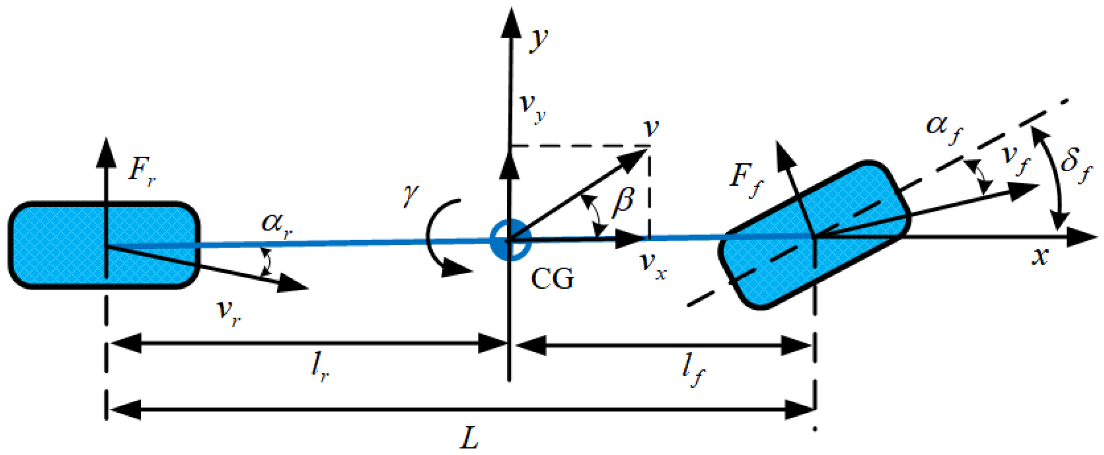
2.2. Model Simplification and Problem Description

Simplification of Coupled Dynamics Model for Intelligent Vehicles

In controller design, using a complex multi-degree-of-freedom intelligent vehicle dynamics model can improve control accuracy. However, the 7-DOF intelligent vehicle model established in this paper involves multiple complex dynamic factors, posing significant challenges to the design and implementation of the controller. Therefore, while ensuring model accuracy, the vehicle model was appropriately simplified to reduce the complexity of the controller design, using a linear two-degree-of-freedom (2-DOF) intelligent vehicle model [26] as the basis for controller design, as shown in Figure 3. The linear 2-DOF intelligent vehicle model has a relatively simple mathematical expression and can effectively describe the two important state variables that directly affect DYC: the sideslip angle and the yaw rate. Therefore, by introducing yaw moment control input based on the 2-DOF model, the simplified model can still meet the requirements of controller design while reducing computational complexity, thereby achieving effective control of vehicle yaw stability.

$$\left\{\begin{array}{l}m\left({\dot{v}}_y+\gamma v_x\right)=F_f\cos {\delta }_f+F_r\\ I_z\dot{\gamma }=l_f{F}_f\cos {\delta }_f-l_r{F}_r+\Delta M\end{array}\right.$$

(11)

$$\left\{\begin{array}{l}{\alpha }_f=-{\delta }_f+\beta +l_f\gamma /v_x\\ {\alpha }_r=\beta -l_r\gamma /v_x\end{array}\right.$$

(12)

Among them, $F_f=C_f{\alpha }_f$ and $F_r=C_r{\alpha }_r$, where $C_f$ and $C_r$ are the lateral stiffness of the front and rear axles, respectively. Assuming the front wheel steering angle is very small, then $\cos {\delta }_f\approx 1$ and $\beta \approx v_y/v_x$.

Thus, the linear 2-DOF model is given as follows:

$$\left\{\begin{array}{l}\dot{\beta }={\displaystyle \frac{k_1+k_2}{m{v}_x}}\beta -{\displaystyle \frac{k_1}{m{v}_x}}{\delta }_f+\left({\displaystyle \frac{l_f{k}_1-l_r{k}_2}{m{v_x}^2}}-1\right)\gamma \\ \dot{\gamma }={\displaystyle \frac{l_f{k}_1-l_r{k}_2}{I_z}}\beta +{\displaystyle \frac{{l_f}^2{k}_1-{l_r}^2{k}_2}{I_z{v}_x}}\gamma -{\displaystyle \frac{l_f{k}_1}{I_z}}{\delta }_f+{\displaystyle \frac{1}{I_z}}\Delta M\end{array}\right.$$

(13)

The state variables $x_1=\beta$ and $x_2=\gamma$ and the state equations are defined as follows:

$$\left\{\begin{array}{l}{\dot{x}}_1=f_1\left(x_1\right)+g_1{x}_2\\ {\dot{x}}_2=f_2\left(x_1,\hspace{0.33em}{x}_2\right)+du\\ y=x_1\end{array}\right.$$

(14)

where $f_1\left(x_1\right)={\displaystyle \frac{k_1+k_2}{m{v}_x}}{x}_1-{\displaystyle \frac{k_1}{m{v}_x}}{\delta }_f$, $g_1={\displaystyle \frac{l_f{k}_1-l_r{k}_2}{m{v_x}^2}}-1$, $f_2\left(x_1,\hspace{0.33em}{x}_2\right)={\displaystyle \frac{l_f{k}_1-l_r{k}_2}{I_z}}{x}_1+{\displaystyle \frac{{l_f}^2{k}_1-{l_r}^2{k}_2}{I_z{v}_x}}{x}_2-{\displaystyle \frac{l_f{k}_1}{I_z}}{\delta }_f$, $d={\displaystyle \frac{1}{I_z}}$, $u=\Delta M$.

The control logic in this paper involves designing an upper-level additional yaw moment control law, $u=\Delta M$, through a lower-level additional yaw moment distribution strategy, ensuring that the vehicle’s center of gravity sideslip angle $x_1$ can track the desired trajectory $x_{1d}$. At the same time, it ensures that the error variables $v_i\left(i=1,2\right)$ are constrained within the compact set ${\Omega }_v=\left\{-k_{ai}<v_i<k_{bi}, i=1,2\right\}$ and that the state variables are constrained within the compact set ${\Omega }_x=\left\{-k_{di}<x_i<k_{ci}, i=1,2\right\}$ to guarantee stability.

Assumption 1. 

$x_{1d}$ is the desired tracking signal, and both $x_{1d}$ and its first derivative ${\dot{x}}_{1d}$ are known, smooth, and bounded. There exist normal constants $Y_0$, ${\overline{Y}}_0$, and $Y_1$ such that ${\underset{¯}{Y}}_0\le x_{1d}\le {\overline{Y}}_0$, $\left|{\dot{x}}_{1d}\right|\le Y_1$, $\forall t\ge 0$.

Lemma 1 

([22]). The second-order directive filter used in this paper is defined as

$$\begin{array}{l}{\dot{z}}_{i,1}={\omega }_n{z}_{i,2}\\ {\dot{z}}_{i,2}=-2\zeta {\omega }_n{z}_{i,2}-{\omega }_n\left(z_{i,1}-{\phi }_i\right)\end{array}$$

(15)

where ${\kappa }_i=z_{i,1}$ and ${\dot{\kappa }}_i={\omega }_n{z}_{i,2}$ are the two outputs of the instruction filter; ${\phi }_i$ is the input of the instruction filter. The initial state of the command filter is ${\phi }_i\left(0\right)=z_{i,1}\left(0\right)$, $z_{i,2}\left(0\right)=0$. When $t\ge 0$ is given, if the input signal ${\phi }_i$ satisfies $\left|{\dot{\phi }}_i\right|\le {\rho }_1$, $\left|{\ddot{\phi }}_i\right|\le {\rho }_2$, ${\rho }_1$ and ${\rho }_2$ are normal constants, then for any $\eta >0$, there exist $\zeta \in \left(0,1\right]$ and ${\omega }_n\ge 0$ such that ${\kappa }_i-{\phi }_i\le \eta$, ${\dot{\kappa }}_i-{\dot{\phi }}_i\le \eta$, $i=1,\hspace{0.33em}2,\hspace{0.33em}3$. Theoretically, by adjusting the values of the filter’s damping $\zeta$ and bandwidth ${\omega }_n$, any tracking accuracy can be achieved. The second-order command filter structure is shown in Figure 4.

Lemma 2 

([27]). For any vectors $s_i\in R^n$ and $v_i\in R^n$, if $\left|v_i\right|<s_i$ is satisfied, then the following inequality holds:

$$\log \left({\displaystyle \frac{{s_i}^2}{{s_i}^2-{v_i}^2}}\right)\le {\displaystyle \frac{{s_i}^2}{{s_i}^2-{v_i}^2}}$$

(16)

Lemma 3 

([21]). For any positive functions $k_{ai}$ and $k_{bi}$, $i=1,\cdots ,n$, let $\Gamma :=R^l\times R^n\subset R^{l+n}$ and $B_1:=\left\{\upsilon \in R:-k_{ai}<v_i\left(t\right)<k_{bi},i=1,\cdots ,n,t\ge 0\right\}\subset R^n$ be open sets. Consider system $\dot{\xi }=f\left(\xi ,u\right)$, where $\xi :={\left[f,v_i\right]}^T\in \Gamma$ and $\varphi$ are free state variables, and $v_i$ is a constrained state variable. If $f:=R_{+}\times \Gamma \to R^{l+n}$ is piecewise-continuous and $\xi$ satisfies the local Lipschitz condition, assume that there exist functions $U:R^l\to R_{+}$ and $V_1:B_1\to R_{+}$ that are continuously differentiable and positive definite in their respective domains, then we have

①

when $v_i\to -k_{ai}$ or $v_i\to k_{bi}$, $V_i\left(v_i\right)\to \infty$

②

${\gamma }_1\left(\left|\varphi \right|\right)\le U\left(\varphi \right)\le {\gamma }_2\left(\left|\varphi \right|\right)$

where ${\gamma }_1$ and ${\gamma }_2$ are $k_{\infty }$-class functions. Let $V\left(\xi \right):=V_i\left(v_i\right)+U\left(\varphi \right)$. If the inequality

$$\dot{V}={\displaystyle \frac{\mathsf{\partial }V}{\mathsf{\partial }\xi }}f\le -a_{0}V+b_0$$

(17)

holds and $a_0>0$, $b_0>0$, then for any $t\in \left[0,\infty \right)$, there is $v_i\left(t\right)\in B_1$.

Remark 1. 

For the barrier Lyapunov function $V\left(v_i\right)$, in the set $\Phi$, when $v_i\to -k_{ai}$ or $v_i\to k_{bi}$, there exists $V\left(v_i\right)\to \infty$. Here, the values of $k_{ai}$ and $k_{bi}$ can either be equal ($k_{ai}=k_{bi}$), in which case it is called a symmetric barrier Lyapunov function, or they can be unequal ($k_{ai}\ne k_{bi}$), in which case it is called an asymmetric barrier Lyapunov function.

Remark 2. 

The necessary conditions for the state error constraint boundaries $k_{ai}$ and $k_{bi}$ are as follows: (1) they must be monotonically decreasing and greater than zero; (2) as $t\to \infty$ , they must converge to a stable value; and (3) for any $t\ge 0$, their derivatives must exist and be bounded above and below.

3. Design and Stability Analysis of a State-Constrained Command-Filtered Controller for Vehicle Yaw Stability

3.1. Controller Design

The error variable is defined as

$$e_1=x_1-x_{1d}, e_2=x_2-{\kappa }_1$$

(18)

where ${\kappa }_1$ represents the output signal of the command filter.

The compensated tracking error subsystem is selected as

$$v_1=e_1-{\tau }_1, v_2=e_2-{\tau }_2$$

(19)

where ${\tau }_i\left(i=1,\hspace{0.33em}2\right)$ are the selected filter error compensation signal. A compact set ${\Omega }_v=\left\{-k_{ai}<v_i<k_{bi},\hspace{0.33em}i=1,\hspace{0.33em}2\right\}$ is defined, and $k_{bi}$ is a constant.

Differentiating Equation (19) yields

$${\dot{v}}_1={\dot{x}}_1-{\dot{x}}_{1d}-{\dot{\tau }}_1$$

(20)

Step 1: For the first error subsystem $v_1$, select an asymmetric barrier Lyapunov function:

$$V_1\left(v_1\right)={\displaystyle \frac{\left(1-q_1\right)}{2}}\ln \left({\displaystyle \frac{{k_{a1}}^2}{{k_{a1}}^2-{v_1}^2}}\right)+{\displaystyle \frac{q_1}{2}}\ln \left({\displaystyle \frac{{k_{b1}}^2}{{k_{b1}}^2-{v_1}^2}}\right)$$

(21)

Differentiating Equation (21) yields

$$\begin{array}{l}{\dot{V}}_1\left(v_1\right)=\left(1-q_1\right){\displaystyle \frac{v_1{\dot{v}}_1}{{k_{a1}}^2-{v_1}^2}}+q_1{\displaystyle \frac{v_1{\dot{v}}_1}{{k_{b1}}^2-{v_1}^2}}\\ =\left({\displaystyle \frac{1-q_1}{{k_{a1}}^2-{v_1}^2}}+{\displaystyle \frac{q_1}{{k_{b1}}^2-{v_1}^2}}\right)v_1{\dot{v}}_1\\ =\left({\displaystyle \frac{1-q_1}{{k_{a1}}^2-{v_1}^2}}+{\displaystyle \frac{q_1}{{k_{b1}}^2-{v_1}^2}}\right)v_1\left({\dot{x}}_1-{\dot{x}}_{1d}-{\dot{\tau }}_1\right)\\ =T_1{v}_1\left({\dot{x}}_1-{\dot{x}}_{1d}-{\dot{\tau }}_1\right)\end{array}$$

(22)

where $q_1=\left\{\begin{array}{l}1,\hspace{0.33em}\hspace{0.33em}0<v_1<k_{b1}\hspace{0.33em}\\ 0,\hspace{0.33em}\hspace{0.33em}-k_{a1}<v_1<0\end{array}\right.$, $T_1=\left({\displaystyle \frac{1-q_1}{{k_{a1}}^2-{v_1}^2}}+{\displaystyle \frac{q_1}{{k_{b1}}^2-{v_1}^2}}\right)$.

Select the virtual control law as

$${\alpha }_1={\displaystyle \frac{1}{g_1}}\left(-k_1{e}_1-f_1\left(x_1\right)+{\dot{x}}_{1d}\right)$$

(23)

Select the error compensation signal as

$${\dot{\tau }}_1=-k_1{\tau }_1+g_1\left({\kappa }_1-{\alpha }_1\right)+g_1{\tau }_2$$

(24)

Substituting (23) and (24) yields

$$\begin{array}{l}{\dot{V}}_1\left(v_1\right)=T_1{v}_1\left({\dot{x}}_1-{\dot{x}}_{1d}-{\dot{\tau }}_1\right)\\ =T_1{v}_1\left(f_1\left(x_1\right)+g_1{x}_2-{\dot{x}}_{1d}+k_1{\tau }_1-g_1\left({\kappa }_1-{\alpha }_1\right)-g_1{\tau }_2\right)\\ =T_1{v}_1\left(f_1\left(x_1\right)+g_1{x}_2-{\dot{x}}_{1d}+k_1{\tau }_1-g_1\left({\kappa }_1-{\displaystyle \frac{1}{g_1}}\left(-k_1{e}_1-f_1\left(x_1\right)+{\dot{x}}_{1d}\right)\right)-g_1{\tau }_2\right)\\ =T_1{v}_1\left(f_1\left(x_1\right)+g_1{x}_2-{\dot{x}}_{1d}+k_1{\tau }_1-g_1{\kappa }_1+\left(-k_1{e}_1-f_1\left(x_1\right)+{\dot{x}}_{1d}\right)-g_1{\tau }_2\right)\\ =T_1{v}_1\left(g_1\left(x_2-{\kappa }_1\right)+k_1\left({\tau }_1-e_1\right)-g_1{\tau }_2\right)\\ =T_1{v}_1\left(g_1{e}_2-k_1{v}_1-g_1{\tau }_2\right)\\ =-k_1{T}_1{v_1}^2+T_1{v}_1{v}_2{g}_1\end{array}$$

(25)

Step 2: For the second error subsystem $v_2$, select an asymmetric barrier Lyapunov function:

$$V_2\left(v_1,\hspace{0.33em}{v}_2\right)=V_1\left(v_1\right)+{\displaystyle \frac{\left(1-q_2\right)}{2}}\ln \left({\displaystyle \frac{{k_{a2}}^2}{{k_{a2}}^2-{v_2}^2}}\right)+{\displaystyle \frac{q_2}{2}}\ln \left({\displaystyle \frac{{k_{b2}}^2}{{k_{b2}}^2-{v_2}^2}}\right)$$

(26)

Taking the derivative of Equation (26) yields

$$\begin{array}{l}{\dot{V}}_2\left(v_1,\hspace{0.33em}{v}_2\right)={\dot{V}}_1\left(v_1\right)+\left({\displaystyle \frac{1-q_2}{{k_{a2}}^2-{v_2}^2}}+{\displaystyle \frac{q_2}{{k_{b2}}^2-{v_2}^2}}\right)v_2{\dot{v}}_2\\ ={\dot{V}}_1\left(v_1\right)+\left({\displaystyle \frac{1-q_2}{{k_{a2}}^2-{v_2}^2}}+{\displaystyle \frac{q_2}{{k_{b2}}^2-{v_2}^2}}\right)v_2\left({\dot{e}}_2-{\dot{\tau }}_2\right)\\ =-k_1{T}_1{v_1}^2+T_1{v}_1{v}_2{g}_1+\left({\displaystyle \frac{1-q_2}{{k_{a2}}^2-{v_2}^2}}+{\displaystyle \frac{q_2}{{k_{b2}}^2-{v_2}^2}}\right)v_2\left({\dot{x}}_2-{\dot{\kappa }}_1-{\dot{\tau }}_2\right)\\ =-k_1{T}_1{v_1}^2+T_1{v}_1{v}_2{g}_1+\left({\displaystyle \frac{1-q_2}{{k_{a2}}^2-{v_2}^2}}+{\displaystyle \frac{q_2}{{k_{b2}}^2-{v_2}^2}}\right)v_2\left(f_2\left(x_1,x_2\right)+du-{\dot{\kappa }}_1\right)\\ =-k_1{T}_1{v_1}^2+T_1{v}_1{v}_2{g}_1+T_2{v}_2\left(f_2\left(x_1,x_2\right)+du-{\dot{\kappa }}_1\right)\end{array}$$

(27)

where $q_2=\left\{\begin{array}{l}1,\hspace{0.33em}\hspace{0.33em}0<v_2<k_{b2}\hspace{0.33em}\\ 0,\hspace{0.33em}\hspace{0.33em}-k_{a2}<v_2<0\end{array}\right.$, $T_2=\left({\displaystyle \frac{1-q_2}{{k_{a2}}^2-{v_2}^2}}+{\displaystyle \frac{q_2}{{k_{b2}}^2-{v_2}^2}}\right)$.

Select the final control law $u$ as

$$u={\displaystyle \frac{1}{d}}\left(-k_2{v}_2-{\displaystyle \frac{T_1{g}_1}{T_2}}{v}_1-f_2\left(x_1,x_2\right)+{\dot{\kappa }}_1\right)$$

(28)

Substituting Equation (28) into Equation (27) yields

$$\dot{V}\left(v_1,\hspace{0.33em}{v}_2\right)=-k_1{T}_1{v_1}^2-k_2{T}_2{v_2}^2$$

(29)

3.2. Stability Analysis

The system’s initial conditions are defined as $-k_{ai}\left(0\right)<v_i\left(0\right)<k_{bi}\left(0\right)$, and the asymmetric barrier Lyapunov function for the entire system is selected.

$$V={\displaystyle \frac{\left(1-q_1\right)}{2}}\ln \left({\displaystyle \frac{{k_{a1}}^2}{{k_{a1}}^2-{v_1}^2}}\right)+{\displaystyle \frac{q_2}{2}}\ln \left({\displaystyle \frac{{k_{b1}}^2}{{k_{b1}}^2-{v_1}^2}}\right)+{\displaystyle \frac{\left(1-q_2\right)}{2}}\ln \left({\displaystyle \frac{{k_{a2}}^2}{{k_{a2}}^2-{v_2}^2}}\right)+{\displaystyle \frac{q_2}{2}}\ln \left({\displaystyle \frac{{k_{b2}}^2}{{k_{b2}}^2-{v_2}^2}}\right)$$

(30)

From Equation (29), we can derive

$$\dot{V}=-k_1{T}_1{v_1}^2-k_2{T}_2{v_2}^2$$

(31)

From Lemma 2, we can derive Equation (32)

$$\dot{V}\le -k_1\left[\ln \left({\displaystyle \frac{{k_{a1}}^2}{{k_{a1}}^2-{v_1}^2}}\right)+\ln \left({\displaystyle \frac{{k_{b1}}^2}{{k_{b1}}^2-{v_1}^2}}\right)\right]-k_2\left[\ln \left({\displaystyle \frac{{k_{a2}}^2}{{k_{a2}}^2-{v_2}^2}}\right)+\ln \left({\displaystyle \frac{{k_{b2}}^2}{{k_{b2}}^2-{v_2}^2}}\right)\right]$$

(32)

Substituting Equation (30) into Equation (32) yields

$$\dot{V}\le -\epsilon V$$

(33)

where $\epsilon =2\min \left\{{\displaystyle \frac{k_1}{1-q_1}},\hspace{0.33em}{\displaystyle \frac{k_1}{q_1}},\hspace{0.33em}{\displaystyle \frac{k_1}{1-q_2}},\hspace{0.33em}{\displaystyle \frac{k_1}{q_2}},\hspace{0.33em}{\displaystyle \frac{k_2}{1-q_1}},\hspace{0.33em}{\displaystyle \frac{k_2}{q_1}},\hspace{0.33em}{\displaystyle \frac{k_2}{1-q_2}},\hspace{0.33em}{\displaystyle \frac{k_2}{q_2}}\right\}$.

From Equation (33), we can obtain

$${\displaystyle \frac{d\left[V\left(t\right)\right]}{dt}}\le -\epsilon \left[V\left(t\right)\right],\hspace{0.33em}\forall \hspace{0.33em}t>0$$

(34)

Multiply both sides of Equation (34) by $e^{\epsilon t}$, and then integrate over the interval $\left(0,t\right]$ to obtain

$$V\left(t\right)\le \left[V\left(0\right)\right]e^{-\epsilon t}\le V\left(0\right),\hspace{0.33em}\forall \hspace{0.33em}t>0$$

(35)

Further obtain

$$-k_{ai}\sqrt{1-e^{-2V\left(0\right)}}\le v_i\le k_{bi}\sqrt{1-e^{-2V\left(0\right)}}$$

(36)

Since $e_i=v_i+{\tau }_i$ and according to Reference [28] $\left|{\tau }_i\right|$ is bounded, suppose $\left|{\tau }_i\right|\le \chi$, where $\chi$ is a positive constant. Then, $-k_{ai}\sqrt{1-e^{-2V\left(0\right)}}-\chi \le e_i\le k_{bi}\sqrt{1-e^{-2V\left(0\right)}}+\chi$. Moreover, the defined Lyapunov function $V$ is also bounded. Since $v_1=e_1-{\tau }_1$ and $-k_{a1}<v_1<k_{b1}$, it follows that $-k_{a1}+\left|{\tau }_1\right|<\left|v_1\right|+\left|{\tau }_1\right|<k_{b1}+\left|{\tau }_1\right|$. Given that $e_1=x_1-x_{1d}$ and $\left|x_{1d}\right|\le Y_0$, we obtain $-k_{a1}\sqrt{1-e^{-2V\left(0\right)}}-\chi -Y_0\le x_1\le k_{b1}\sqrt{1-e^{-2V\left(0\right)}}+\chi +Y_0$. Since ${\kappa }_1$ is a function of $e_1$ and ${\dot{x}}_{1d}$, it is bounded. Let ${\kappa }_1$ satisfy $\left|{\kappa }_1\right|\le {\overline{\kappa }}_1$, where ${\overline{\kappa }}_1$ is a positive constant. Furthermore, since $v_2=e_2-{\tau }_2$ and $-k_{a2}\le v_2\le k_{b2}$, we obtain $-k_{a2}+\left|{\tau }_2\right|<\left|v_2\right|+\left|{\tau }_2\right|<k_{b2}+\left|{\tau }_2\right|$. Given that $e_2=x_2-{\kappa }_1$, it follows that $-k_{a2}\sqrt{1-e^{-2V\left(0\right)}}-\chi -{\overline{\kappa }}_1\le x_2\le k_{b2}\sqrt{1-e^{-2V\left(0\right)}}+\chi +{\overline{\kappa }}_1$. In summary, the system state variables $x_i$ are constrained within the compact set ${\Omega }_v=\left\{-k_{di}<x_i<k_{ci}, i=1,2\right\}$.

4. Distribution of Additional Lateral Yaw Moment in the Lower Layer

In the yaw stability command-filtered control of intelligent vehicles based on state constraints, the additional yaw moment $\Delta M$ obtained from calculations needs to be appropriately distributed to the four wheels in the form of braking torque. Compared to single-wheel braking, applying braking torque to the wheels on one side can generate a greater yaw moment, enhance overall vehicle stability, and reduce the load on individual tires. The distribution rules for the wheels on one side are presented in

Table 1. Braking rules for single-side wheels.

${\mathbf{\delta }}_{\mathit{f}}$	Category	$\mathit{\Delta }\mathit{M}$	Acting Brake
${\delta }_f>0$	Oversteer	$\_$	Right-side wheel
${\delta }_f>0$	Understeer	$+$	Left-side wheel
${\delta }_f<0$	Understeer	$+$	Right-side wheel
${\delta }_f<0$	Oversteer	$+$	Left-side wheel

.

Assuming the left wheel is controlled separately,

$$\Delta M\approx {\displaystyle \frac{B_f}{2}}{F}_{L\_fl}+{\displaystyle \frac{B_r}{2}}{F}_{L\_rl}$$

(37)

Considering that the steering angle ${\delta }_f$ of the vehicle is relatively small and that the difference between the front and rear wheelbases of the vehicle is also very small, Equation (37) can be written as

$${\displaystyle \frac{\Delta M}{\left(B_f+B_r\right)/4}}\approx F_{B\_fl}+F_{B\_rl}$$

(38)

where $F_{B\_fl}$ and $F_{B\_rl}$ represent the braking forces of the left front wheel and the left rear wheel, respectively.

Changes in the vertical load on the tire can cause variations in the tire’s lateral stiffness, which in turn affects the stability of the vehicle. Here, it is assumed that when the wheels are not locked, the tire braking force is approximately proportional to its vertical load, and the dynamic distribution of braking force is carried out according to the following formula:

$$\left\{\begin{array}{l}{F}_{B\_fl}={\displaystyle \frac{F_{Z\_fl}}{F_{Z\_fl}+F_{Z\_rl}}}{\displaystyle \frac{\Delta M}{\left(B_f+B_r\right)/4}}\\ F_{B\_rl}={\displaystyle \frac{F_{Z\_rl}}{F_{Z\_fl}+F_{Z\_rl}}}{\displaystyle \frac{\Delta M}{\left(B_f+B_r\right)/4}}\end{array}\right.$$

(39)

The left wheel requires a braking torque provided by the brake

$$\left\{\begin{array}{l}{T}_{B\_fl}={\displaystyle \frac{F_{Z\_fl}}{F_{Z\_fl}+F_{Z\_rl}}}{\displaystyle \frac{\Delta M}{\left(B_f+B_r\right)/4}}R\\ T_{B\_rl}={\displaystyle \frac{F_{Z\_rl}}{F_{Z\_fl}+F_{Z\_rl}}}{\displaystyle \frac{\Delta M}{\left(B_f+B_r\right)/4}}R\end{array}\right.$$

(40)

Similarly, the braking torque of the front and rear wheels on the right side of the car can be calculated as

$$\left\{\begin{array}{l}{T}_{B\_fr}={\displaystyle \frac{F_{Z\_fr}}{F_{Z\_fr}+F_{Z\_rr}}}{\displaystyle \frac{\Delta M}{\left(B_f+B_r\right)/4}}R\\ T_{B\_rr}={\displaystyle \frac{F_{Z\_rr}}{F_{Z\_fr}+F_{Z\_rr}}}{\displaystyle \frac{\Delta M}{\left(B_f+B_r\right)/4}}R\end{array}\right.$$

(41)

5. Simulation Verification and Result Analysis

5.1. Yaw Stability Control Process of Intelligent Vehicles

Figure 5 illustrates the yaw stability control architecture for intelligent vehicles. The process initiates with the upper-layer state-constrained command-filtered controller, synthesizing an additional yaw moment $\Delta M$ through real-time compensation of the deviation between the desired and measured centroid sideslip angles. This corrective moment is subsequently distributed via unilateral wheel braking strategies, where braking torque allocation algorithms determine actuation commands for specific wheels, thereby achieving precise yaw motion regulation.

5.2. Parameter Settings

To verify the effectiveness of the proposed state-constrained command-filtered control (SC-CFC), as shown in Figure 6, the method is compared with an uncontrolled (NoControl) intelligent vehicle under the same front-wheel steering conditions on dry asphalt roads (friction coefficient: 0.85) and dry gravel roads (friction coefficient: 0.5). The parameter settings for the intelligent vehicle are as follows: m = 1412 kg; $B_f=B_r$ = 1.675 m; $l_f$ = 1.015 m; $l_r$ = 1.895 m; $h_g$ = 0.54 m; g = 9.8 m/s²; $I_z$ = 1536.7 kg·m²; $J$ = 0.9 kg·m²; $R$ = 0.325 m; $C_f$ = −50,000 N/m; $C_r$ = −50,000 N/m.

Considering the steering characteristics of drivers, the longitudinal velocity direction of intelligent vehicles should be as consistent as possible with the driver’s facing direction. Therefore, this study sets the desired vehicle centroid sideslip angle ${\beta }_d$ to 0 [29]. Research indicates that ordinary drivers with limited driving experience can still maintain normal control when $\beta <2^0$. However, as the sideslip angle further increases, the driver’s control ability may deteriorate, thereby affecting driving safety. Consequently, this study constrains the centroid sideslip angle within $\pm 2^0$ [30]. Moreover, the yaw rate is influenced by vehicle speed and road surface adhesion conditions. Given these constraints, when the yaw rate satisfies $\left|\gamma \right|\le 0.85\left(\mu g/{\nu }_x\right)$ [31], the vehicle can maintain stability within the entire operating range without experiencing loss of control.

As stated in the introduction, the vehicle yaw stability control strategy based on state constraints proposed in this study is applicable to both symmetric and asymmetric conditions. To enhance the adaptability and flexibility of the control algorithm and align with practical application requirements, this study adopts a symmetric constraint form for the parameters $\beta$, $\gamma$, $v_1$, and $v_2$.

5.3. Result Analysis

Operating Condition 1. $v_x$ = 60 km/h, $\mu =0.5$. Controller parameters: $k_1=20$, $k_2=20$, $k_{c1}=0.035$, $k_{d1}=-0.035$, $k_{c2}=0.25$, $k_{d2}=-0.25$, $k_{b1}=0.01$, $k_{a1}=-0.01$, $k_{b2}=0.05$, $k_{a2}=-0.05$, $\xi =0.5$, ${\omega }_n=1000$. The simulation results are shown in Figure 7, Figure 8, Figure 9 and Figure 10.

Figure 6 illustrates the bidirectional step input condition for the front wheel steering angle, where the absolute peak value reaches 0.075 rad. From Figure 7, it can be observed that, under the control of the SC-CFC controller, the centroid sideslip angle of the intelligent vehicle closely follows the desired value. Additionally, during the commanded front wheel steering angle transitions, the state variations in the vehicle remain significantly below its constraint boundaries $k_{c1}$ and $k_{d1}$. In contrast, under uncontrolled conditions, when the front wheel steering angle is relatively large, the amplitude of centroid sideslip angle variation is more pronounced. However, at this moment, the vehicle is still within the stability constraint boundaries. From Figure 8, it can be seen that in the absence of the controller, when the front wheel steering angle is large, the vehicle’s yaw rate approaches its constraint boundaries, indicating a potential risk of vehicle loss of control during steering. Conversely, with the SC-CFC controller, the yaw rate remains constrained within the stable region $k_{c2}$ and $k_{d2}$ throughout the entire control process, effectively ensuring the vehicle’s driving stability. Furthermore, from Figure 9 and Figure 10, it is evident that the filtering errors $\left\{\left.v_i\right|i=1,2\right\}$ remain within the constraint boundaries throughout the process, verifying the effectiveness of the SC-CFC controller.

Operating Condition 2. $v_x=90\mathrm{km}/\mathrm{h}$, $\mu =0.85$. Controller parameters: $k_1=12$, $k_2=12$, $k_{c1}=0.035$, $k_{d1}=-0.035$, $k_{c2}=0.28$, $k_{d2}=-0.28$, $k_{b1}=0.02$, $k_{a1}=-0.02$, $k_{b2}=0.15$, $k_{a2}=-0.15$, $\xi =0.5$, ${\omega }_n=1000$. The simulation results are shown in Figure 11, Figure 12, Figure 13 and Figure 14.

In Operating Condition 2, the front wheel steering angle input remains the same as in Operating Condition 1. From Figure 11, it can be observed that, under the control of the SC-CFC controller, the centroid sideslip angle of the intelligent vehicle closely follows the desired value. Additionally, during the commanded front wheel steering angle return for lane change, the vehicle’s state variables remain consistently below their constraint boundaries $k_{c1}$ and $k_{d1}$. However, under uncontrolled conditions, when the front wheel steering angle is relatively large, the variation in centroid sideslip angle increases significantly, even exceeding the stability constraint boundary. This indicates that the intelligent vehicle is highly prone to instability in this scenario, posing a considerable risk of traffic accidents. From Figure 12, further validation can be obtained: under uncontrolled conditions, when the front wheel steering angle is large, the yaw rate essentially approaches its constraint boundaries, further demonstrating the high likelihood of vehicle loss of control. Conversely, under the control of the SC-CFC controller, although the yaw rate exhibits some oscillations throughout the process, it remains constrained within the stable region $k_{c2}$ and $k_{d2}$ at all times, effectively ensuring vehicle driving stability. Similarly, from Figure 13 and Figure 14, it can be observed that the filtering errors $\left\{\left.v_i\right|i=1,2\right\}$ remain constrained within the specified boundaries throughout the entire process.

The simulation results of Operating Conditions 1 and 2 indicate that the yaw stability command-filtered control strategy based on state constraints can effectively constrain the filtering errors $\left\{\left.v_i\right|i=1,2\right\}$ and state variables $\left\{\left.x_i\right|i=1,2\right\}$ within the compact sets ${\Omega }_v=\left\{-k_{ai}<v_i<k_{bi}, i=1,2\right\}$ and ${\Omega }_x=\left\{-k_{di}<x_i<k_{ci}, i=1,2\right\}$. This verifies the correctness and effectiveness of the proposed control algorithm. Compared to the uncontrolled scenario, this control strategy shows significant advantages in enhancing vehicle yaw stability.

6. Conclusions

This study focuses on the yaw stability control of intelligent vehicles. A comprehensive full-vehicle dynamic model and a simplified 2-DOF dynamic model are established. Under the premise of satisfying necessary assumptions, a state-constrained yaw stability command-filtered control method is proposed. This method introduces a BLF to effectively constrain two key state variables: the sideslip angle and the yaw rate, thereby enhancing system stability and safety. Meanwhile, a CFC approach is adopted to reduce computational complexity, and an error compensation mechanism is incorporated to mitigate the adverse effects of filter-induced errors on system performance. To validate the effectiveness and robustness of the proposed control method, simulations are conducted under different vehicle speeds on both dry asphalt and dry gravel road surfaces. The simulation results demonstrate that the proposed method effectively ensures vehicle yaw stability, providing valuable insights for the practical application of yaw stability control in intelligent vehicles.

References

1. Liu, J.; Liu, J. Intelligent and Connected Vehicles: Current Situation, Future Directions, and Challenges. IEEE Commun. Mag. 2018, 2, 59–65. [Google Scholar] [CrossRef]
2. Cao, X.; Huang, K.; Lian, Y.; Tian, Y. Direct Yaw Moment Control of Electric Vehicle for Improving the Vehicle Lateral Stability. In Proceedings of the 2018 IEEE International Conference on Mechatronics and Automation (ICMA), Changchun, China, 5–8 August 2018. [Google Scholar]
3. Pi, D.; Chen, N.; Zhang, B.; Zhong, G. Enhancements in vehicle stability with yaw moment control via differential braking. In Proceedings of the 2009 IEEE International Conference on Vehicular Electronics and Safety (ICVES), Pune, India, 11–12 November 2009. [Google Scholar]
4. Wang, B.; Zhang, J.; Zhang, Y.; Wang, W. The direct yaw-moment control based on adaptive fuzzy LQR for distributed drive electric vehicles. Adv. Mech. Eng. 2024, 16, 16878132241273524. [Google Scholar] [CrossRef]
5. Kong, X.; Deng, Z.; Zhao, Y.; Gao, W. Stability control of distributed drive electric vehicle based on adaptive fuzzy sliding mode. Proc. Inst. Mech. Eng. Part D J. Automob. Eng. 2024, 238, 2741–2752. [Google Scholar] [CrossRef]
6. Sun, C.; Xu, Z.; Deng, S.; Tong, B. Integration sliding mode control for vehicle yaw and rollover stability based on nonlinear observation. Trans. Inst. Meas. Control 2022, 44, 3039–3056. [Google Scholar] [CrossRef]
7. Ding, S.; Liu, L.; Zheng, W. Sliding Mode Direct Yaw-Moment Control Design for In-Wheel Electric Vehicles. IEEE Trans. Ind. Electron. 2017, 64, 6752–6762. [Google Scholar] [CrossRef]
8. Liu, C.; Liu, H.; Han, L.; Wang, W.; Guo, C. Multi-Level Coordinated Yaw Stability Control Based on Sliding Mode Predictive Control for Distributed Drive Electric Vehicles Under Extreme Conditions. IEEE Trans. Veh. 2022, 72, 280–296. [Google Scholar] [CrossRef]
9. Li, J.; Luo, J.; Feng, B.; Zhang, L.; Gao, M. Vehicle stability control based on vehicle motion state and tire force estimation. Trans. Can. Soc. Mech. Eng. 2024. [Google Scholar] [CrossRef]
10. Liang, J.; Feng, J.; Lu, Y.; Yin, G.; Zhuang, W.; Mao, X. A Direct Yaw Moment Control Framework Through Robust T-S Fuzzy Approach Considering Vehicle Stability Margin. IEEE/ASME Trans. Mechatron. 2023, 29, 166–178. [Google Scholar] [CrossRef]
11. Zhang, J.; Sun, W.; Feng, Z. Vehicle yaw stability control via H∞ gain scheduling. Mech. Syst. Signal Process. 2018, 106, 62–75. [Google Scholar] [CrossRef]
12. Chen, J.; Liu, Y.; Liu, R.; Xiao, F.; Huang, J. Integrated control of braking-yaw-roll stability under steering-braking conditions. Sci. Rep. 2023, 13, 21110. [Google Scholar] [CrossRef]
13. Jin, L.; Zhou, H.; Xie, X.; Guo, B.; Ma, X. A direct yaw moment control frame through model predictive control considering vehicle trajectory tracking performance and handling stability for autonomous driving. Control Eng. Pract. 2024, 148, 105947. [Google Scholar] [CrossRef]
14. Guo, N.; Lenzo, B.; Zhang, X.; Zou, Y.; Zhai, R.; Zhang, T. A Real-Time Nonlinear Model Predictive Controller for Yaw Motion Optimization of Distributed Drive Electric Vehicles. IEEE Trans. Veh. Technol. 2020, 69, 4935–4946. [Google Scholar] [CrossRef]
15. Ileš, Š.; Švec, M.; Makarun, P.; Hromatko, J. Predictive direct yaw moment control with active steering based on polytopic linear parameter-varying model. In Proceedings of the 2022 8th International Conference on Control, Decision and Information Technologies (CoDIT), Istanbul, Turkey, 17–20 May 2022. [Google Scholar]
16. Rini, G.; Mazzilli, V.; Bottiglione, F.; Gruber, P.; Dhaens, M.; Sorniotti, A. On Nonlinear Model Predictive Vehicle Dynamics Control for Multi-Actuated Car-Semitrailer Configurations. IEEE Access 2024, 12, 165928–165947. [Google Scholar] [CrossRef]
17. Alyoussef, F.; Kaya, I. A review on nonlinear control approaches: Sliding mode control backsteping control and feedback linearization control. In Proceedings of the International Engineering and Natural Sciences Conference (IENSC 2019), Diyarbakir, Turkey, 6–8 November 2019. [Google Scholar]
18. Pang, H.; Yao, R.; Wang, P.; Xu, Z. Adaptive backsteping robust tracking control for stabilizing lateral dynamics of electric vehicles with uncertain parameters and external disturbances. Control Eng. Pract. 2021, 110, 104781. [Google Scholar] [CrossRef]
19. Park, G. Sideslip angle control of electronic-four-wheel drive vehicle using backsteping controller. Int. J. Automot. Technol. 2022, 23, 729–739. [Google Scholar] [CrossRef]
20. He, Y.; King, E.; Cai, Y.; Yuan, C. Design and analysis of robust state constraint control for direct yaw moment control system. Int. J. Model. Simul. 2022, 42, 551–560. [Google Scholar] [CrossRef]
21. Tee, K.; Ge, S.; Tay, E.H. Barrier Lyapunov functions for the control of output-constrained nonlinear systems. Automatica 2009, 45, 918–927. [Google Scholar] [CrossRef]
22. Farrel, J.; Polycarpou, M.; Sharma, M.; Dong, W. Command filtered backstepping. IEEE Trans. Autom. Control 2009, 54, 1391–1395. [Google Scholar] [CrossRef]
23. Liu, W.; Zhao, H.; Shen, H.; Xu, S.; Park, J. Command-filter Based Predefined-time Control for State-constrained Nonlinear Systems Subject to Preassigned Performance Metrics. IEEE Trans. Autom. 2024, 69, 7801–7807. [Google Scholar] [CrossRef]
24. Hao, R.; Wang, H.; Zheng, W. Time-varying state constrained estimators-based command filtered quantized consensus control for nonlinear multiagent systems. Int. J. Robust Nonlinear Control 2023, 33, 11306–11334. [Google Scholar] [CrossRef]
25. Zhang, T.; Feng, C. Command filter-based adaptive event-triggered control for switched nonlinear systems with full state constraints. Int. J. Robust Nonlinear Control 2024, 34, 3873–3890. [Google Scholar] [CrossRef]
26. Masato, A. Vehicle Handling Dynamics: Theory and Application; Butterworth-Heinemann: Oxford, UK, 2015. [Google Scholar]
27. Ren, B.; Ge, S.; Tee, K.; Lee, T. Adaptive Neural Control for Output Feedback Nonlinear Systems Using a Barrier Lyapunov Function. IEEE Trans. Neural Netw. 2010, 21, 1339–1345. [Google Scholar] [PubMed]
28. Yu, J.; Shi, P.; Zhao, L. Finite-time command filtered backstepping control for a class of nonlinear systems. Automatica 2018, 92, 173–180. [Google Scholar] [CrossRef]
29. Shino, M.; Miyamoto, N.; Wang, Y.; Nagai, M. Traction control of electric vehicles considering vehicle stability. In Proceedings of the 6th International Workshop on Advanced Motion Control, Nagoya, Japan, 30 March–1 April 2000. [Google Scholar]
30. Liu, W.; Ding, H.; Guo, K.; Zhou, B. Application of Side-Slip Angle Phasigram to Vehicle ESC System. Trans. Beijing Inst. Technol. 2013, 33, 42–46. [Google Scholar]
31. Ulsoy, A.; Peng, H.; Çakmakci, M. Automotive Control Systems; Cambridge University Press: Cambridge, UK, 2012. [Google Scholar]
Figure 1. 7-DOF dynamic model of an intelligent vehicle.
Actuators 14 00148 g001
Figure 2. Wheel model.
Actuators 14 00148 g002
Figure 3. 2-DOF model.
Actuators 14 00148 g003
Figure 4. Structure of the second-order command filter.
Actuators 14 00148 g004
Figure 5. Yaw stability control process of intelligent vehicles.
Actuators 14 00148 g005
Figure 6. Front wheel steering angle δ f .
Actuators 14 00148 g006
Figure 7. Sideslip angle β .
Actuators 14 00148 g007
Figure 8. Yaw rate γ .
Actuators 14 00148 g008
Figure 9. Filtering error v 1 .
Actuators 14 00148 g009
Figure 10. Filtering error v 2 .
Actuators 14 00148 g010
Figure 11. Sideslip angle β .
Actuators 14 00148 g011
Figure 12. Yaw rate γ .
Actuators 14 00148 g012
Figure 13. Filtering error v 1 .
Actuators 14 00148 g013
Figure 14. Filtering error v 2 .
Actuators 14 00148 g014