Research on Viewpoints Planning for Industrial Robot-Based Three-Dimensional Sculpture Reconstruction

Abstract

To improve the accuracy and completeness of three-dimensional sculpture reconstruction, this study proposes a global–local two-step scanning method for industrial robot-based scanning. First, a global model is generated through stepped rotary scanning based on the object’s dimensions. Subsequently, local viewpoint planning is conducted to refine regions that were incompletely captured in the initial step, with a genetic algorithm optimizing the scanning paths to enhance efficiency. The local models are then aligned and fused with the global model to produce the final 3D reconstruction. Comparative experiments on sculptures made of different materials were conducted to validate the effectiveness of the proposed method. Compared with CAD-slicing and surface-partitioning methods, the proposed approach achieved superior model completeness, a scanning accuracy of 0.26 mm, a standard deviation of 0.31 mm, and a total scanning time of 152 s. The results indicate that the proposed method enhances reconstruction integrity and overall quality while maintaining high efficiency, making it a viable approach for high-precision 3D surface inspection tasks.

1. Introduction

The development of three-dimensional (3D) sculptures has a long history. They serve as carriers of art and culture, witnesses to history, and custodians of cultural heritage, possessing significant artistic and cultural value. Obtaining digital models of these sculptures using three-dimensional measurement equipment is of great importance. This process not only facilitates the conservation, restoration, and reproduction of these works but also enables the analysis of their structures and supports further design and innovation. Moreover, digital models can be used to create virtual art galleries, promoting the dissemination and exchange of cultural heritage [1,2,3].

In recent years, the integration of robots and 3D scanning equipment has gained widespread application in fields such as reverse engineering, industrial inspection, and heritage conservation, due to its advantages of non-contact operation, high efficiency, high accuracy, and repeatability [4,5,6]. However, limitations in the scanner’s field of view, depth, and angle mean that a single viewpoint can capture only part of a large object’s surface. As a result, multiple scanning viewpoints must be carefully planned. Most existing robotic 3D scanning systems rely on manual viewpoint demonstrations to measure objects. It is not only labor-intensive and empirically challenging, but also, it makes it difficult to ensure the quality, efficiency, and completeness of the scan. Additionally, due to the lack of prior knowledge regarding the geometry and structural dimensions of the object, scanning viewpoints are often planned through estimation. This increases the complexity of the associated algorithms and makes it more challenging to obtain comprehensive data. Therefore, developing effective methods for robotic-scanning-viewpoint planning is crucial for accurate 3D measurement of three-dimensional crafted objects.

The scanning viewpoint planning without a priori information about the object to reconstruct has been studied by many scholars. Karaszewski et al. [6] employed initial, rough, and fine measurements to ensure the integrity of the scan model for automatic measurement of cultural heritage objects, such as large sculptures, and planned a collision-free scan path using inverse kinematics. Kwon et al. [7] obtained a rough model by exploring the motion and then generated hemispherical scan paths for rescanning in areas with large errors and areas with missing scans. Lee et al. [8] proposed an automatic pose generation method where the object’s shape is inferred from initial detection, the scanning viewpoint is determined, and the scanning path is then planned using local confidence assessment. Ozkan et al. [9] proposed a 3D reconstruction method for surface contour-guided scanning of unknown objects. In this method, the scanning viewpoint location is determined from the sampled points in the image passing through the convex hull’s center of mass. The viewpoint orientation is then calculated based on the center of the turntable and the center of mass of the sampled points. A secondary complementary scan is performed to capture the missing areas. Peng et al. [10] proposed a viewpoint-planning algorithm based on estimated occupancy probability, which controls overlap to enhance scan coverage and improve integrity. Yuan et al. [11] used mass vector chain (MVCs) for viewpoint planning, where the next viewpoint is determined by the inverse of the current point cloud ensemble vector, with the ensemble vector being 0 as the planning termination condition. Martins et al. [12] used an incremental model to represent the object’s surface and workspace occupancy, calculating the optimal scan viewpoint and a collision-free scan trajectory. Li et al. [13] used mass vector chains (MVCs) and boundary integrals of vector fields to determine the next best view (NBV), enabling the planning of both the observation direction and the sensor’s precise position in space. Chen et al. [14] modeled the object’s trend surface using surface curvature to predict unknown areas and determine the next viewpoint. Munkelt et al. [15] divided viewpoint planning into two stages: in the first stage, the number of visible voxels is maximized to build a general model of the object quickly with guaranteed accuracy; in the second stage, secondary scanning is performed for occluded voxels and low accuracy voxels in the model to improve the model quality. Zhou et al. [16] used maximum information from the visible surface to predict unscanned areas and determine the visibility of the next viewpoint. Kriegel et al. [17,18] reconstructed the data stream obtained from real-time acquisition into a 3D surface and generated scan paths based on surface trends in its boundary regions. Irving et al. [19] used a utility function to evaluate the goodness of the candidate views and reduced the time to compute the NBV by a multi-resolution search strategy and finally dealt with the uncertainty of localization by re-evaluating the neighboring views based on the real candidate views.

In summary, despite the development of various algorithms, existing scanning-viewpoint-planning methods are often complex and can result in incomplete models, particularly when the object shape is intricate or when key areas are not fully captured in the initial scan. To address this challenge, this study proposes a global–local two-step scanning method to enhance the accuracy and completeness of 3D sculpture reconstruction. Initially, a global model is generated using stepped rotary scanning, and then local viewpoint planning is performed to refine regions with incomplete data, ensuring higher reconstruction fidelity. The genetic algorithm is employed to optimize scanning paths, improving scanning efficiency and enhancing model integrity, making it a viable approach for high-precision 3D surface inspection tasks.

To address these challenges, a two-step scanning-based viewpoint-planning method is proposed. The paper is organized as follows: Section 2 introduces the stepped-rotary scanning-viewpoint planning for constructing the global model; Section 3 presents the local fine-scale viewpoint planning for detailed scanning; Section 4 outlines the experimental setup and discusses the results; Section 5 concludes with a summary of the findings and offers an outlook for future work.

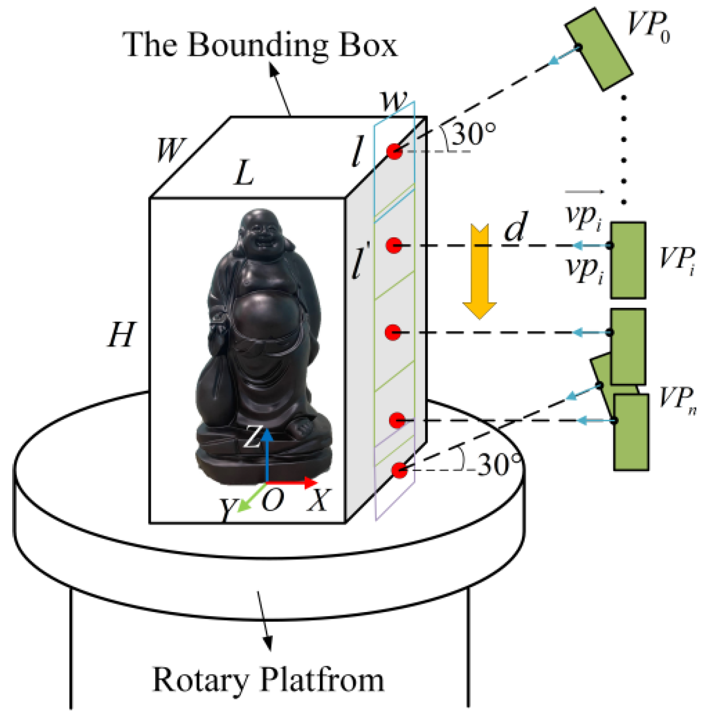
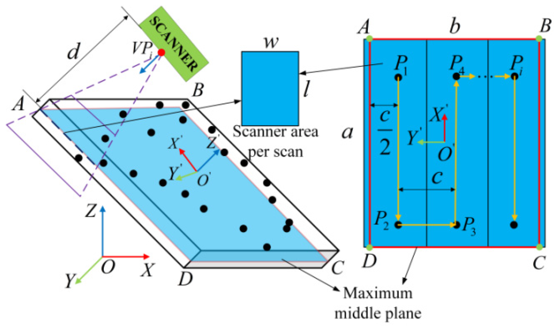
2. Global Viewpoints Planning for Global Model

In the absence of detailed information regarding the object’s size and contour, a global rough model is proposed to capture the surface contour through stepped rotary scanning. This method is inspired by the manual scanning process conducted around the workpiece, as shown in Figure 1.

First, the minimum bounding box is obtained by manually measuring the object’s length, width, and height (L × W × H). Based on this bounding box, the scanning viewpoints are planned: The scanner begins at the initial viewpoint (VP₀) at the top of the bounding box. The turntable completes one full rotation, after which the scanning head proceeds to the next viewpoint. The turntable continues to rotate one full revolution, and this process is repeated until all viewpoints are covered.

To effectively scan both the top and bottom surfaces of the object, the initial(VP₀) and final (VP_n) viewpoints are positioned at a 30° angle relative to the XOY plane. The set of scanned viewpoints $\mathrm{VP}=\{V{P}_i:v{p}_i(x_i,y_i,z_i),\overrightarrow{v{p}_i}(n_{ix},n_{iy},n_{iz})|i=0,1,2\cdots n\}$:

$$k=⌈{\displaystyle \frac{H}{l}}⌉;n=k+2;l^{\prime }={\displaystyle \frac{H}{k}}$$

(1)

$$V{P}_0:\left\{\begin{array}{l}v{p}_0(x_0={\displaystyle \frac{L}{2}}+d*\cos 30°,y_0=0,z_0=H+d*\sin 30°)\\ \overrightarrow{v{p}_0}(n_{0x}=-{\displaystyle \frac{1}{\cos 30°}},n_{0y}=0,n_{0z}=-{\displaystyle \frac{1}{\sin 30°}})\end{array}\right.$$

(2)

$$V{P}_n:\left\{\begin{array}{l}v{p}_n(x_n={\displaystyle \frac{L}{2}}+d*\cos 30°,y_n=0,z_n=d*\sin 30°)\\ \overrightarrow{v{p}_n}(n_{nx}=-{\displaystyle \frac{1}{\cos 30°}},n_{ny}=0,n_{nz}=-{\displaystyle \frac{1}{\sin 30°}})\end{array}\right.$$

(3)

$$V{P}_i:\left\{\begin{array}{l}v{p}_i(x_i={\displaystyle \frac{L}{2}}+d,y_0=0,z_0=H-l^{\prime }*i)\\ \overrightarrow{v{p}_i}(n_{ix}=-1,n_{0y}=0,n_{0z}=0) i=1,2,3\cdots n-1\end{array}\right.$$

(4)

where vp_i is the position of the viewpoint VP_i, $\overrightarrow{v{p}_i}$ is the scanning direction of the viewpoint VP_i, l is the length of a single scan of the scanner, and d is the scanning distance.

3. Local Viewpoints Planning for Local Models

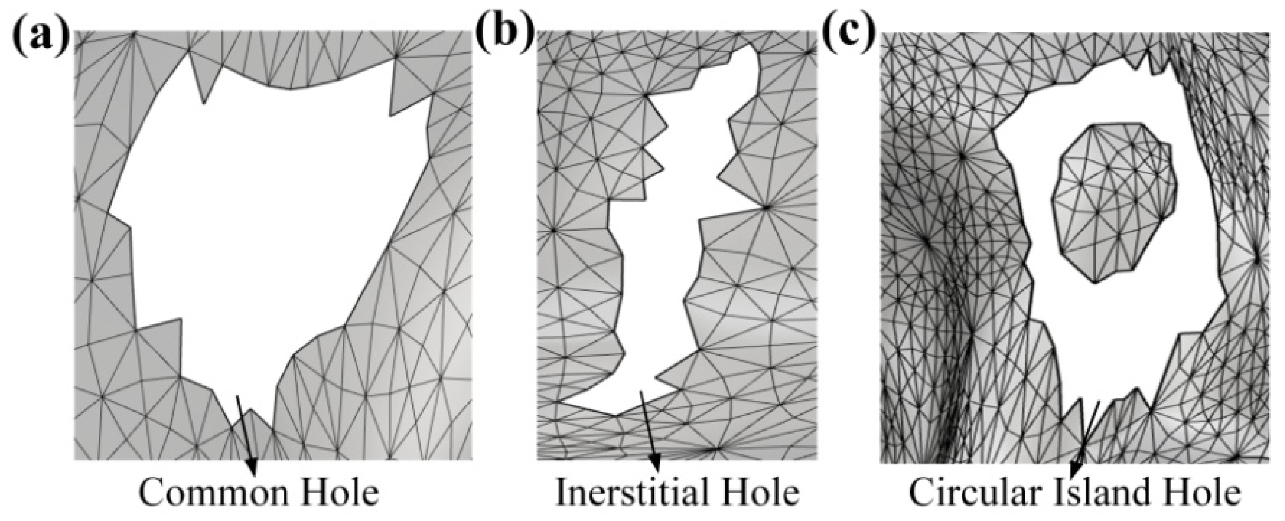
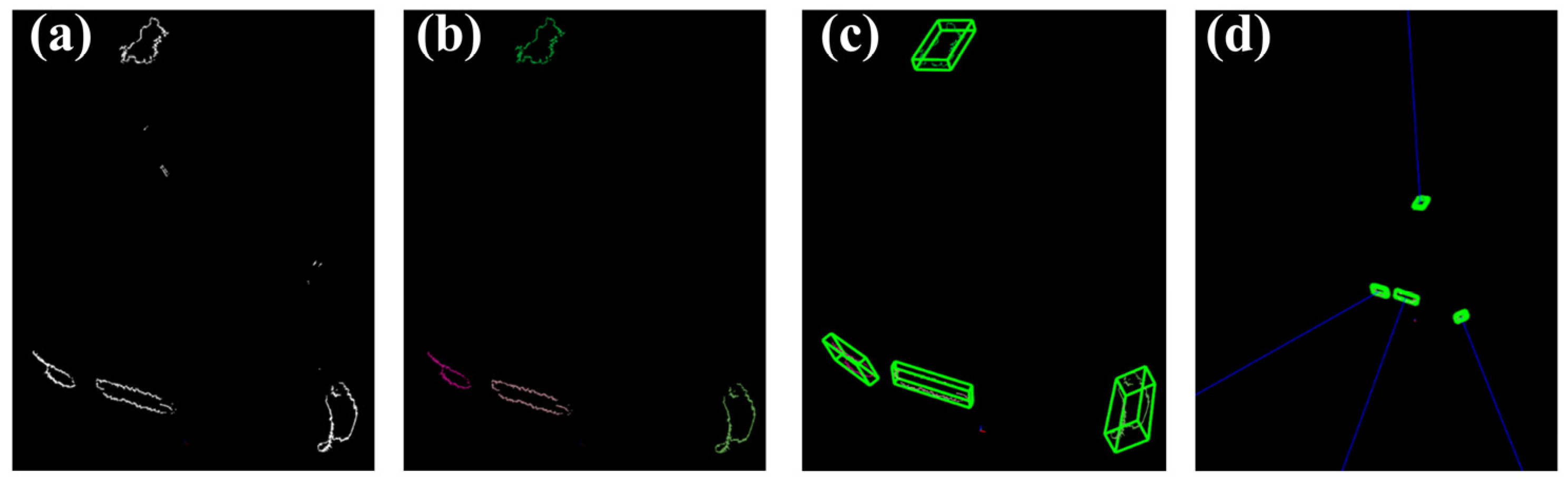
3.1. Left Holes Recognition After Global Scanning

Most of the digitized models obtained after the global scanning process contain areas with missing 3D information, commonly referred to as holes. These holes can be attributed to two main causes. First, during the point cloud data collection process, limitations in the measurement system, the complex and variable shape of the workpiece surface, and external environmental factors during scanning can result in missing data in the point cloud, leading to holes in the scanned model. Second, during the point-cloud-processing stage, poor data quality can contribute to the formation of holes in the reconstructed mesh model. These localized holes can directly impact the accuracy and integrity of the object’s mesh model. To address this issue, a finer second scan is required to fill the gaps, ensuring the model’s completeness and quality.

The boundary of a hole in a model provides information about its location and shape. Based on the position of the holes within the model, the local holes of a scanned and processed mesh model can be classified into two categories: edge holes and internal holes, as shown in Figure 2. Edge holes are characterized by open boundaries located along the model’s exterior, while internal holes have closed boundaries situated within the interior of the model.

Internal holes can be further categorized into common holes, interstitial holes, and circular island holes based on their shape, as shown in Figure 3a–c. Common holes have a regularly shaped, closed boundary. Interstitial holes feature a narrow and elongated closed boundary. Circular island holes, on the other hand, have a circular boundary and contain isolated island-like facets within the hole.

Due to the closed spatial nature of the objects scanned in this study, no edge holes appear in the mesh model generated after the global scanning process. Additionally, annular island holes are absent because the point cloud data from the global scan undergoes outlier removal, eliminating isolated points that would otherwise form such holes. As a result, the mesh model produced by the global scan only contains common holes and interstitial holes.

To accurately determine the position of each local hole, it is necessary to first identify the hole area. A method for identifying hole boundaries based on a point cloud model is proposed. The grid model, generated through stepwise rotation scanning, is converted into a point cloud model. Hole boundaries are identified by analyzing the normal angles of points in the point cloud and their neighbors.

Before calculating the normal vector for each data point, the neighborhood relationship between points needs to be constructed. There are two common types of adjacency between points in discrete point clouds. One is the radius R-nearest neighbor, that is, the set of all points $N_P^r$ within the ball, with point P as the center and r as the radius, as illustrated in Figure 4a. The second is the K-nearest neighbor, i.e., the set $N_P^k$ of k points nearest to point P, with point P as the origin, as illustrated in Figure 4b. Since the points of the $N_P^k$ nearest-neighbor set are biased towards the denser side, which is not conducive to the accuracy of subsequent hole boundary point identification, therefore, the radius R-nearest neighbor approach is used to define the neighborhood of the scattered point cloud.

To enable the rapid identification of neighboring point sets, topological relations for scattered point clouds must be established. A k-d tree is employed to spatially partition the point cloud data and efficiently determine the radius R-nearest neighbors of a point within the local space.

The point cloud normal vector forms the foundation for hole identification. Since the point cloud model obtained from the scanner contains only three-dimensional position information, normal vectors must be computed for each point. To accomplish this, a local surface-fitting method is used to estimate the normals. Notably, the normal directions, derived from the covariance matrix of neighboring points, exhibit ambiguity—some normals point inward, while others point outward. A minimum spanning tree combined with depth-first traversal is employed to ensure the consistent orientation of the point cloud normals.

To identify hole boundary feature points, the uniformity of the distribution of a data point P and its $N_P^r$ neighboring points is analyzed to determine whether P is a boundary feature point. The uniformity is evaluated using the maximum angle principle. The basic idea is that if the neighborhood set $N_P^r$ of point P is distributed on one side, then P is a hole boundary feature, as shown in Figure 5a; on the contrary, if the neighborhood point set $N_P^r$ is evenly distributed around P, then P is an internal point, as shown in Figure 5b.

Once the data point P(x₀,y₀,z₀) and its normal n(a,b,c) are known, a normal vector plane S can be defined with the following plane equation:

$$a(x-x_0)+b(y-y_0)+c(z-z_0)=0$$

(5)

Projecting the set $\{P_i(x_i,y_i,z_i)|i=1,2,\cdots ,k\}$ of $N_P^r$ neighborhood points of the data point P onto this normal vector plane gives the projection point ${P_i}^{\prime }(i=1,2,\cdots ,k)$, as shown in Figure 6a; the coordinates of the projection point ${P_i}^{\prime }({x_i}^{\prime },{y_i}^{\prime },{z_i}^{\prime })$ are the following:

$$\begin{array}{l}{x_i}^{\prime }={\displaystyle \frac{a(a{x}_0+b{y}_0+c{z}_0)+(b^2+c^2)x_i-ab{y}_i-ac{z}_i}{a^2+b^2+c^2}}\\ {y_i}^{\prime }=\left\{\begin{array}{cc}{\displaystyle \frac{b}{a}}({x_i}^{\prime }-x_i)+y_i& a\ne 0\\ y_i& a=0\end{array}\right.\\ {z_i}^{\prime }=\left\{\begin{array}{cc}{\displaystyle \frac{c}{a}}({x_i}^{\prime }-x_i)+z_i& a\ne 0\\ z_i& a=0\end{array}\right.\end{array}$$

(6)

After finding the coordinates of the projection points, a projection point ${P_i}^{\prime }$ is randomly selected, and a vector $P{P_i}^{\prime }$ is constructed and then sorted clockwise, as shown in Figure 6b.

Calculate the angle between the two adjacent vectors $P{P_i}^{\prime }$ and $P{P^{\prime }}_{i+1}$ from the clockwise direction ${\alpha }_i(i=1,2,\cdots ,k)$:

$$\begin{array}{c}{\alpha }_i=\arccos ({\displaystyle \frac{P{P_i}^{\prime }\cdot P{P^{\prime }}_{i+1}}{\left|P{P_i}^{\prime }\right|*\left|P{P^{\prime }}_{i+1}\right|}})\\ \left|P{P_i}^{\prime }\right|=\sqrt{{({x^{\prime }}_i-x_0)}^2+{({y^{\prime }}_i-y_0)}^2+{({z^{\prime }}_i-z_0)}^2}\\ \left|P{P^{\prime }}_{i+1}\right|=\sqrt{{({x^{\prime }}_{i+1}-x_0)}^2+{({y^{\prime }}_{i+1}-y_0)}^2+{({z^{\prime }}_{i+1}-z_0)}^2}\\ P{P_i}^{\prime }\cdot P{P^{\prime }}_{i+1}=({x^{\prime }}_i-x_0)({x^{\prime }}_{i+1}-x_0)+({y^{\prime }}_i-y_0)({y^{\prime }}_{i+1}-y_0)+({z^{\prime }}_i-z_0)({z^{\prime }}_{i+1}-z_0)\end{array}$$

(7)

The maximum vector angle α_max is found and compared with a predefined threshold. If smaller than the threshold, the data point P is classified as an interior point; otherwise, it is identified as a hole boundary feature. The threshold is typically determined by the spatial complexity and distribution density of the point cloud. Setting the threshold to π/4 resulted in more accurate identification of hole boundary feature points.

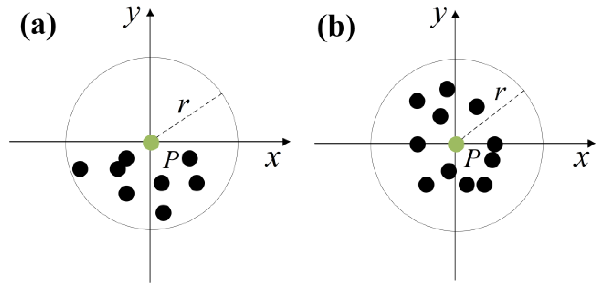
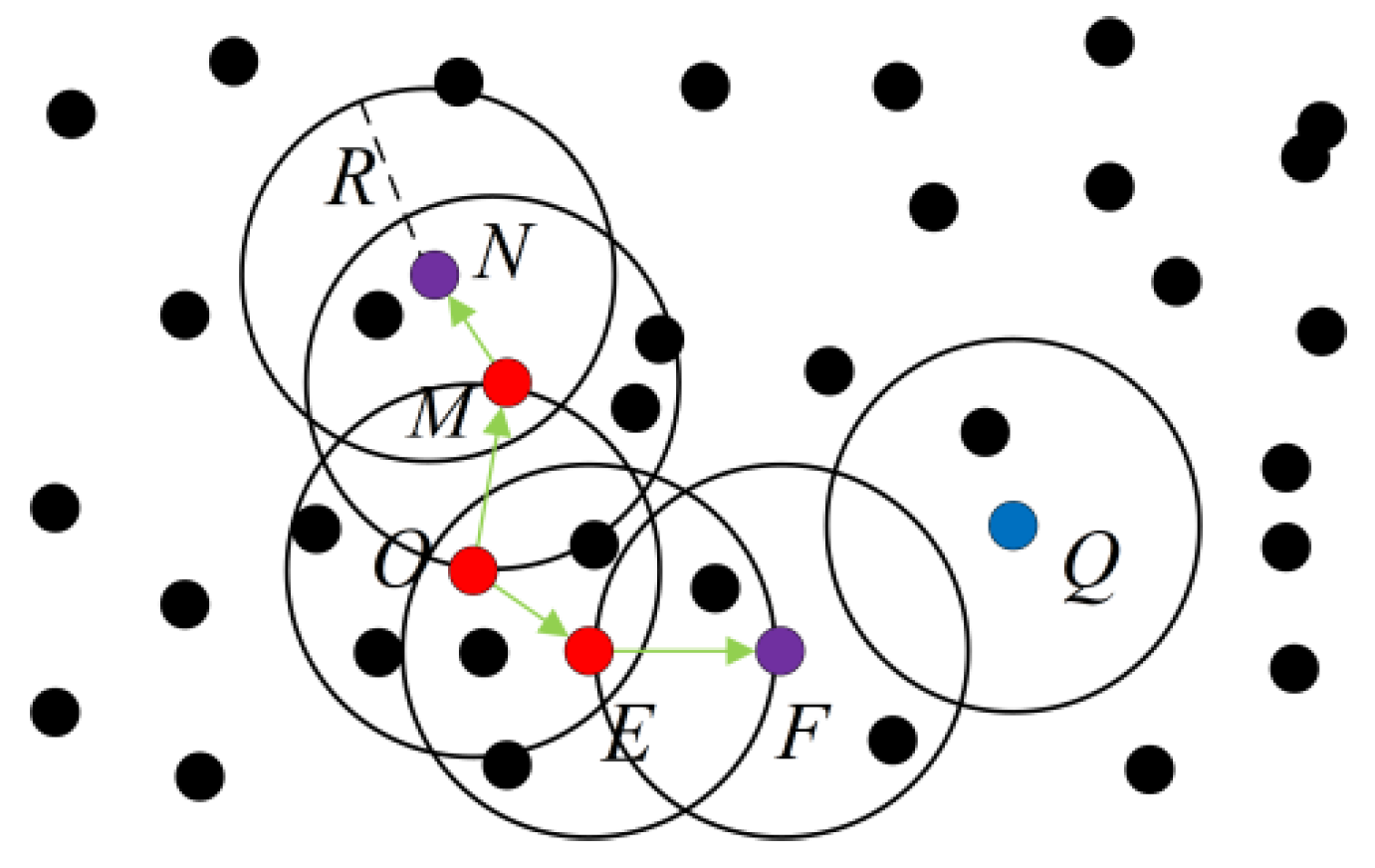
3.2. Holes Clustering

The identified hole boundary feature points in the point cloud model must be clustered to determine both the number of holes and the set of individual boundary feature points. These feature points exhibit characteristics such as a small data volume and significant density variation, which makes DBSCAN [20] an ideal choice for clustering. DBSCAN is a density-based algorithm that does not require a predefined number of clusters. It identifies anomalous points as noise and efficiently scans clusters of arbitrary size and shape based on the spatial density of the data points. Therefore, this study uses the DBSCAN algorithm to cluster the hole boundary feature points.

The DBSCAN clustering algorithm classifies spatial data points into three types: noise points, boundary points, and core points. It defines the relationships between spatial data points as density-connected, density-direct, and density-reachable. Assuming the data set $D=\{x_1,x_2,\cdots ,x_m\}$, the specific density is defined as follows:

(1)

ε-neighborhood: $\forall x_j\in D$, ε-neighborhood contains a subset of sample set D consisting of points no farther than ε from x_j, i.e., $N_{\epsilon }(x_j)=\{x_i\in D|dist(x_i,x_j)\le \epsilon \}$. The number of subsamples in this subset is denoted as $|N_{\epsilon }(x_j)|$;

(2)

Core point: $\forall x_j\in D$, if ε-neighborhood of x_j contains at least MinPts of samples, i.e., then x_j is a core point;

(3)

Boundary point: a point falls within the ε-neighborhood of a core point;

(4)

Noise point: a point that is neither a core point nor a boundary point is considered a noise point;

(5)

Density direct: if x_j is in the ε-neighborhood of x_i and x_i is a core point, then x_j is said to be density direct from x_i;

(6)

Density reachable: for x_j and x_i, x_j is said to be density-reachable by x_i if there exists a sequence of samples p₁, p₂, ∙∙∙, p_n, where p_{1 =} x_i, p_{n =} x_j, and p_i+1 is directly density-reachable from p_i;

(7)

Density connected: For x_j and x_i, x_j and x_i are said to be connected if there exists x_k such that both x_j and x_i are accessible by x_k density.

To illustrate the above concepts, an example is provided, as shown in Figure 7. Where Minpts = 5, neighborhood radius R, red points O, E, and M are core points, purple points N and F are boundary points, and blue point Q is a noise point. E and M are O density-direct, N is M density-direct, F is E density-direct, N and F are O density-reachable, and N and F are density-connected.

The core concept of the DBSCAN clustering algorithm is to identify core points and the sample points that are directly reachable from these core points within a specified ε-neighborhood and a minimum number of sample points, MinPts. The algorithm then assigns all core points to clusters, while classifying sample points that do not belong to any cluster as noise. The specific steps are as follows:

Assume that the data consist of a sample point set $D=(x_1,x_2,\cdots ,x_m)$, a neighborhood parameter $(\epsilon ,MinPts)$, and a cluster family C.

(1)

Initialize the set of core points $\Omega =\varnothing$, the number of clusters k = 0, and initialize the set of unvisited samples $\Gamma =D$. The clusters are then divided into $\mathrm{C}=\varnothing$;

(2)

For $j=1,2,\cdots ,m$, find all the core points as follows:

(a)

Find the ε-neighborhood subsample set $N_{\epsilon }(x_j)$ of sample x_j using the distance metric;

(b)

If the number of samples in the subsample set satisfies $|N_{\epsilon }(x_j)|\ge MinPts$, add sample x_j to the set of core points: $\Omega =\Omega \cup \left\{x_j\right\}$;

(3)

If the set of core points $\Omega =\varnothing$, the algorithm is finished; otherwise, proceed to step (4);

(4)

Select a random core point $o$ from the core point set $\Omega$, initialize the current cluster core point queue ${\Omega }_{cur}=\left\{o\right\}$, initialize the current cluster sample set $C_k=\left\{o\right\}$, and update the unvisited sample set $\Gamma =\Gamma -\left\{o\right\}$;

(5)

If the current cluster core point queue ${\Omega }_{cur}=\varnothing$, generate the current cluster C_k, update the cluster division $\mathrm{C}=\{C_1,C_2,\cdots ,C_k\}$, update the core point set $\Omega =\Omega -C_k$, and proceed to step (3). Otherwise, update the core point set $\Omega =\Omega -C_k$;

(6)

Remove a core point $o^{\prime }$ from the current cluster core point queue ${\Omega }_{cur}$, pass the neighborhood distance threshold ε-neighborhood sub-sample set $N_{\epsilon }(o^{\prime })$, make $\Delta =N\epsilon (o^{\prime })\cap \Gamma$, update the current cluster sample set $C_k=C_k\cup \Delta$, update the unvisited sample set $\Gamma =\Gamma -\Delta$, update ${\Omega }_{cur}={\Omega }_{cur}\cup (\Delta \cap \Omega )-o^{\prime }$, and proceed to step (5).

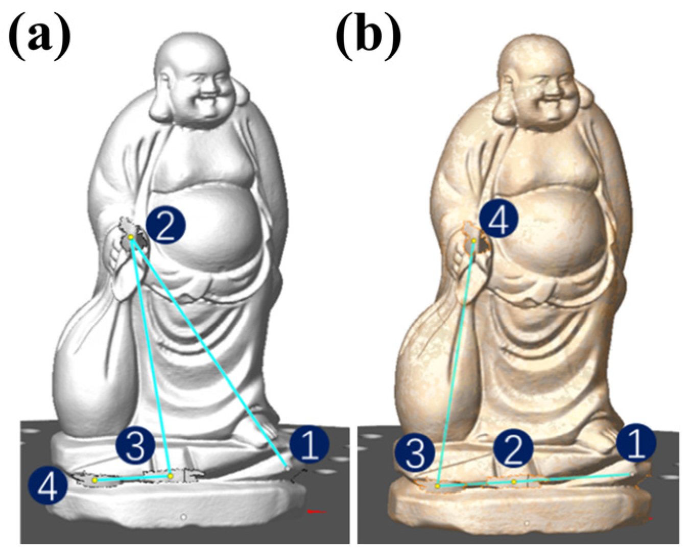
3.3. Local Viewpoints Planning

To improve the efficiency and convenience of viewpoint planning for local holes, the corresponding viewpoint is calculated based on the size of the enclosing bounding box. The bounding-box methods are used to determine the optimal enclosing space for a set of discrete points. Typical examples include the Bounding Sphere (BS), Axis-Aligned Bounding Box (AABB), Oriented Bounding Box (OBB), and Fixed Directions Hulls (FDHs), as illustrated in Figure 8.

Since the OBB algorithm [21] provides good spatial tightness and allows the bounding box to rotate along with the geometric object, it is utilized for each hole boundary feature point set. The scanning viewpoint of the hole area is then determined based on the maximum middle plane of the OBB and the scanning area of the scanner. The relationship between the dimensions (a × b) of the maximum middle plane of the OBB and the dimensions (l × w) of a single scan area of the scanner can be categorized into four cases, as illustrated in Figure 9a–d.

As shown in Figure 10, when the length and width of the largest middle plane of the OBB envelope box at the boundary of the hole is less than the length and width of the scanner in a single scan, only one scan is required to sweep the entire area of the hole. Therefore, only one scanning viewpoint needs to be planned. Coordinates of the position of scanning viewpoint $VP\{vp(x,y,z),\overrightarrow{vp}(n_x,n_y,n_z)\}$ in the O-XYZ coordinate system:

$$\overrightarrow{vp}=-\overrightarrow{O^{\prime }{Z}^{\prime }}$$

(8)

$$vp={}_{O^{\prime }}{}^{O}R*v{p}_{O^{\prime }-X^{\prime }{Y}^{\prime }{Z}^{\prime }}+{O^{\prime }}_{O-XYZ}$$

(9)

where $\overrightarrow{O^{\prime }{Z}^{\prime }}\left(x_{Z^{\prime }},y_{Z^{\prime }},z_{Z^{\prime }}\right)$ is the unit vector of the Z’ axis of the O’-X’Y’Z’ coordinate system, ${}_{O^{\prime }}{}^{O}R$ is the rotation matrix of O’-X’Y’Z’ with respect to the O-XYZ coordinate system, and ${O^{\prime }}_{O-XYZ}$ are the coordinates of the center point O’ of the OBB-enclosing box under O-XYZ. The above parameters are obtained when calculating the OBB-enclosing box, $v{p}_{O^{\prime }-X^{\prime }{Y}^{\prime }{Z}^{\prime }}(0,0,d)$ are the coordinates of the position of the viewpoint VP under the O’-X’Y’Z’ coordinate system, and d is the scanning distance.

As shown in Figure 11, when the length of the largest middle plane of the OBB envelope box at the boundary of the hole is less than the length of the scanner in a single scan and the width is greater than the width of the scanner in a single scan, the hole area can be swept in its entirety by simply moving the scan horizontally. Therefore, only two scanning viewpoints need to be planned. Calculate the scanning direction $\overrightarrow{vp}$ and the coordinate value $v{p}^{\prime }(x^{\prime },y^{\prime },z^{\prime })$ in the O’-X’Y’Z’ coordinate system for the scanning viewpoints VP₁ and VP₂:

$$\overrightarrow{v{p}_1}=\overrightarrow{v{p}_2}=-\overrightarrow{O^{\prime }{Z}^{\prime }}$$

(10)

$$\left\{\begin{array}{l}{x}_1^{\prime }=0\\ y_1^{\prime }=y_A+{\displaystyle \frac{w}{2}}\\ z_1^{\prime }=d\end{array}\right. \left\{\begin{array}{l}{x}_2^{\prime }=0\\ y_2^{\prime }=-y_1^{\prime }\\ z_2^{\prime }=d\end{array}\right.$$

(11)

Once the coordinates of the viewpoint in the O’-X’Y’Z’ coordinate system have been obtained, the coordinates of the position of the scanned viewpoint $V{P}_i\{i=1,2\}$ in the O-XYZ coordinate system $v{p}_i(x_i,y_i,z_i)$ can be obtained according to Equation (9).

As shown in Figure 12, when the maximum middle plane of the OBB envelope at the boundary of the hole is longer than the length of the scanner in a single scan and wider than the width of the scanner in a single scan, the hole area can be scanned in its entirety by simply moving the scan vertically. In this case, again, only two scanning viewpoints need to be planned. Similarly to the above calculation procedure, the scan directions $\overrightarrow{vp}$ for VP₁ and VP₂ and the coordinate values $v{p}^{\prime }(x^{\prime },y^{\prime },z^{\prime })$ in the O’-X’Y’Z’ coordinate system:

$$\overrightarrow{v{p}_1}=\overrightarrow{v{p}_2}=-\overrightarrow{O^{\prime }{Z}^{\prime }}$$

(12)

$$\left\{\begin{array}{l}{x}_1^{\prime }=x_A-{\displaystyle \frac{l}{2}}\\ y_1^{\prime }=0\\ z_1^{\prime }=d\end{array}\right. \left\{\begin{array}{l}{x}_2^{\prime }=-x_1^{\prime }\\ y_2^{\prime }=0\\ z_2^{\prime }=d\end{array}\right.$$

(13)

Also, according to Equation (9), the coordinates of the position of the scanned viewpoint $V{P}_i\{i=1,2\}$ in the O-XYZ coordinate system can be obtained as $v{p}_i(x_i,y_i,z_i)$.

As shown in Figure 13, when the length and width of a single scan by the scanner are less than the length and width of the maximum middle plane of the OBB envelope box, multiple scanning viewpoints need to be planned to ensure that the full hole area is swept.

Firstly, determine the total number of scanned viewpoints:

$$n=2⌈{\displaystyle \frac{b}{w}}⌉ n>2$$

(14)

Based on the number of scanned viewpoints determined, the scanning distance can be obtained as follows:

$$c={\displaystyle \frac{2b}{n}}$$

(15)

Coordinates of the sampling point $P_i({x_i}^P,{y_i}^P,{z_i}^P)$ on its largest intermediate plane in the O’-X’Y’Z’ coordinate system:

$$\left\{\begin{array}{l}{x_1}^P=x_A-{\displaystyle \frac{l}{2}}\\ {y_1}^P=y_A-{\displaystyle \frac{c}{2}}\\ {z_1}^P=0\end{array}\right. i=1$$

(16)

$$\left\{\begin{array}{l}ifi\mathrm{mod}2=0 {x_i}^P=-{x_{i-1}}^P,{y_i}^P={y_{i-1}}^P,{z_i}^P=0\\ ifi\mathrm{mod}2\ne 0 {x_i}^P={x_{i-1}}^P,{y_i}^P={y_{i-1}}^P-c,{z_i}^P=0\end{array}\right. i=2,3,\cdots ,n$$

(17)

where $A(x_A,y_A,0)$ is a vertex on the maximum middle plane.

After obtaining the sample point $P_i({x_i}^P,{y_i}^P,{z_i}^P)$, the scanning direction ${\overrightarrow{vp}}_i$ and the coordinates of the position $v{p}_i^{\prime }(x_i^{\prime },y_i^{\prime },z_i^{\prime })$ in the O’-X’Y’Z’ coordinate system can be calculated for the scanning viewpoint $V{P}_i\{v{p}_i(x_i,y_i,z_i),\overrightarrow{v{p}_i}(n_{ix},n_{iy},n_{iz})\}$:

$$\overrightarrow{v{p}_i}=-\overrightarrow{O^{\prime }{Z}^{\prime }}$$

(18)

$${\displaystyle \frac{\overrightarrow{O^{\prime }{Z}^{\prime }}}{{\overrightarrow{P_{i}VP}}_i}}={\displaystyle \frac{1}{d}}\left\{\begin{array}{l}{x}_i^{\prime }={x_i}^P\\ y_i^{\prime }={y_i}^P\\ z_i^{\prime }=d\end{array}\right.$$

(19)

Finally, according to Equation (9), the coordinates of the position of the scanned viewpoint $V{P}_i\{i=1,2,\cdots ,n\}$ in the O-XYZ coordinate system are obtained.

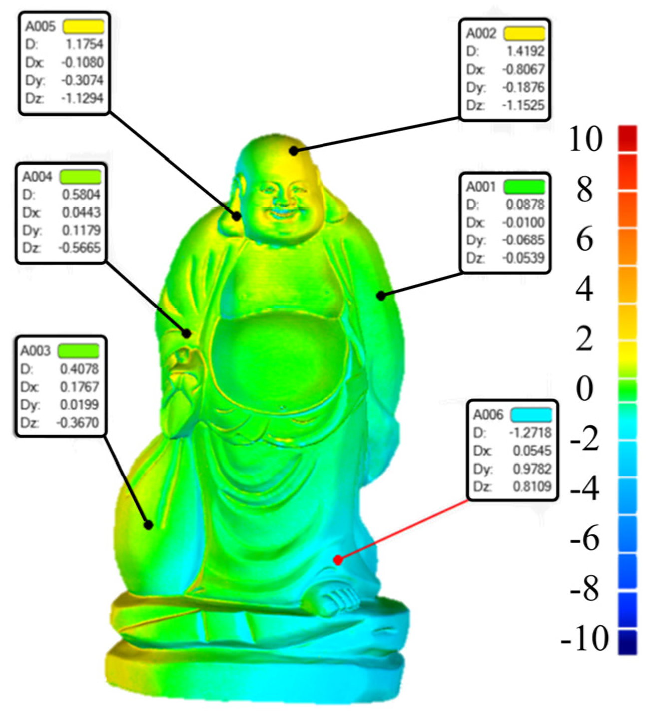
4. Experiment and Discussion

To verify the feasibility and effectiveness of the proposed viewpoint-planning method, an industrial robot-based 3D scanning system was used, as shown in Figure 14. The system consists of a KUKA KR240 R2900 (KUKA Robotics Corporation, Augsburg, Germany) 6-DOF industrial robot, a 3D scanner, a graphics-processing workstation, a V-shaped fixture, a turntable, and other essential components. The industrial robot has a repeated positioning accuracy of ±0.06 mm and a maximum arm span of 2696 mm. The 3D scanner is equipped with a customized V-shaped fixture to facilitate scanning tasks. The workpiece to be scanned is placed on a turntable with a diameter of 1520 mm and a maximum rotational speed of 10 r/min. The performance specifications of the 3D scanner are listed in

Table 1. Performance indicators of 3D scanners.

Key Performance Indicator	Value
Working distance (Zs)	400 ≤ Zs ≤ 1000 mm
Close-range scanning (l1 × w1)	214 × 148 mm
Long-range scanning (l2 × w2)	536 × 371 mm
Scanning-angle range (l × w)	30° × 21°
Highest 3D resolution	0.1 mm
Highest 3D point accuracy	0.05 mm
Maximum 3D distance accuracy	0.03% 100 cm
Maximum 3D reconstruction rate	16 fps
Maximum data acquisition speed	2 × 106 points/s

.

As shown in Figure 15, a 600 mm × 330 mm × 200 mm wood carving was used in the automated scanning experiment. The scanning path was planned using a stepped-rotary-scanning method and then imported into an offline programming software for simulation and optimization.

The scanning-process parameters are provided in

Table 2. Scanning parameters.

Scanning-Process Parameters	Value
Scanning distance	700 mm
Scanning speed	0.1 m/s
Capture frame rate	10 fps
Turntable speed	10 r/min

.

The point cloud model obtained from the stepped rotary scan is pre-processed and 3D reconstructed to generate its global model. Due to impact factors from the scanning system, scanning environment, and the object to reconstruct, the global model may miss data, which manifest as holes. As illustrated in Figure 16, the global model exhibits four distinct holes, marked in red.

The local scan is performed to obtain the missing data from the global scan. The global model was discretized into a point cloud model, which was used for hole identification, clustering, and viewpoint planning as shown in Figure 17a–d.

Once the scan points for a hole are obtained, the scan path is generated by connecting the points in a predefined sequence. To enhance scanning efficiency while considering the space and time complexity of the algorithm, a genetic algorithm is employed to find the shortest scan path for each local scan viewpoint. Figure 18 shows 1–4 scanning points of the holes. Figure 18a shows the random scan path before optimization, while Figure 18b shows the optimized scan path. The initial random scan path has a length of 763.9 mm, which is reduced to 585.7 mm after path optimization. This reduction of approximately 30% in the total scan path length demonstrates an improvement in scanning efficiency, assuming a constant scanning speed.

The planned scan path is imported into the offline programming software for simulation and optimization. For viewpoints where the robot’s articulated arm limits exist, the workpiece is rotated using a rotary table to ensure that all scan viewpoints are safely reachable by the robot. The point cloud obtained from the local scan is processed and subsequently merged with the global scan’s point cloud, as illustrated in Figure 19a. The combined point cloud is then fused to create the final reconstructed object, shown in Figure 19b. To assess the effectiveness of the proposed method, the final reconstruction is compared to the reference model digitized by a coordinate measuring machine (CMM), as depicted in Figure 19c.

The scanning error of 0.77 mm, with a standard deviation of 1.02 mm, is within acceptable limits, with a 100% scan completeness rate and a total scanning time of 202 s. However, the areas with the greatest error, as shown in Figure 20, can be attributed to several factors. These include the precision limitations of the scanning device, which can affect the accuracy in capturing fine details, especially in intricate features. Additionally, errors may arise from the point cloud merging process, where insufficient overlap or imperfect registration of multiple scans can lead to misalignments. Finally, challenges in accurately aligning the scanned data with the reference model, particularly in complex geometries, further contribute to the observed errors in these regions.

To verify the applicability of the method to models of different materials, a white marble sculpture was selected as the test workpiece, as shown in Figure 21. The performance of the proposed algorithm was evaluated by comparing it with the widely used CAD-slicing method [22] and the surface-partitioning method. The model obtained using the proposed algorithm demonstrated a scanning integrity of 100%, a scanning accuracy of 0.26 mm, a standard deviation of 0.31 mm, and a total scanning time of 152 s.

Table 3. Comparison results of three algorithms.

	Scanning Integrity	Scanning Accuracy	Standard Deviation	Scanning Time
CAD-slicing method	89.05%	1.86 mm	2.71 mm	145 s
Surface-partitioning method	97.08%	0.97 mm	1.12 mm	120 s
Two-step scanning method	100%	0.26 mm	0.31 mm	152 s

presents the comparison results of the three algorithms. The test results indicate that the proposed planning algorithm demonstrates superior scanning integrity and quality compared to the original slicing and partitioning methods. Although its scanning efficiency is slightly lower than that of the other two methods, the overall scanning times for all three are comparable. Therefore, the proposed scanning path is both reasonable and effective, yielding complete surface data with high scanning quality, thus meeting the requirements for workpiece surface quality inspection.

5. Conclusions

In this paper, a robotic-scanning-viewpoint-planning method is proposed based on a two-step scanning approach for automated measurement of three-dimensional artifacts. The originality of the method lies in obtaining a global model of the object to reconstruct using a stepwise rotational-scanning-viewpoint-planning technique. Subsequently, local fine scanning viewpoint planning is performed using the DBSCAN clustering algorithm and the OBB algorithm to fill in local holes in the global model caused by missing scan areas. To improve overall scanning efficiency, a genetic algorithm was used to calculate the optimal local fine scanning path. Experiments were conducted using an industrial robot-based 3D scanning system on sculptures made of different materials. The results were compared with those from the CAD-slicing and surface-partitioning methods. The experimental results showed that the proposed method achieved higher scan integrity, with a scanning accuracy of 0.26 mm and a scanning time of 152 s. While the scanning efficiency was slightly lower, the proposed method demonstrated superior scan quality compared to the other methods. Overall, it provided complete, high-quality surface data, meeting the requirements for workpiece inspection.

However, several limitations of the current method warrant further consideration. Notably, the issue of occlusion at scanning viewpoints has not been addressed, and the scanning efficiency may be compromised by frequent reorientation of the robot between different viewpoints. These factors may influence the overall time efficiency and could become more pronounced when scanning more complex or geometrically intricate objects. Future research will focus on mitigating these limitations by developing a viewpoint quality evaluation function, which will incorporate both occlusion and the reorientation of the robot. This enhancement aims to optimize the viewpoint selection process, thereby improving both the quality and efficiency of scanning, and extending the applicability of the proposed method to a wider range of 3D artifacts.

References

1. Pieraccini, M.; Guidi, G.; Atzeni, C. 3D digitizing of cultural heritage. J. Cult. Herit. 2001, 2, 63–70. [Google Scholar] [CrossRef]
2. Zabulis, X.; Meghini, C.; Partarakis, N.; Beisswenger, C.; Dubois, A.; Fasoula, M.; Galanakis, G. Representation and preservation of Heritage Crafts. Sustainability 2020, 12, 1461. [Google Scholar] [CrossRef]
3. Fu, Y. Reflections on the Digital Protection and Dissemination of Traditional Ceramic Handicrafts of Non-Foreign Heritage. Art Perform. Lett. 2023, 4, 78–85. [Google Scholar] [CrossRef]
4. Zhao, Y.; Zhao, J.; Zhang, L.; Qi, L. Development of a robotic 3D scanning system for reverse engineering of freeform part. In Proceedings of the 2008 International Conference on Advanced Computer Theory and Engineering, Phuket, Thailand, 20–22 December 2008; pp. 246–250. [Google Scholar] [CrossRef]
5. Phan, N.D.M.; Quinsat, Y.; Lavernhe, S.; Lartigue, C. Scanner path planning with the control of overlap for part inspection with an industrial robot. Int. J. Adv. Manuf. Technol. 2018, 98, 629–643. [Google Scholar] [CrossRef]
6. Karaszewski, M.; Sitnik, R.; Bunsch, E. On-line, collision-free positioning of a scanner during fully automated three-dimensional measurement of cultural heritage objects. Robot. Auton. Syst. 2012, 60, 1205–1219. [Google Scholar] [CrossRef]
7. Kwon, H.; Na, M.; Song, J.B. Rescan strategy for time efficient view and path planning in automated inspection system. Int. J. Precis. Eng. Manuf. 2019, 20, 1747–1756. [Google Scholar] [CrossRef]
8. Lee, I.D.; Seo, J.H.; Kim, Y.M.; Choi, J.; Han, S.; Yoo, B. Automatic pose generation for robotic 3-D scanning of mechanical parts. IEEE Trans. Robot. 2020, 36, 1219–1238. [Google Scholar] [CrossRef]
9. Ozkan, M.; Secil, S.; Turgut, K.; Dutagaci, H.; Uyanik, C.; Parlaktuna, O. Surface profile-guided scan method for autonomous 3D reconstruction of unknown objects using an industrial robot. Vis. Comput. 2022, 38, 3953–3977. [Google Scholar] [CrossRef]
10. Peng, W.; Wang, Y.; Miao, Z.; Feng, M.; Tang, Y. Viewpoints planning for active 3-D reconstruction of profiled blades using estimated occupancy probabilities (EOP). IEEE Trans. Ind. Electron. 2020, 68, 4109–4119. [Google Scholar] [CrossRef]
11. Yuan, X. A mechanism of automatic 3D object modeling. IEEE Trans. Pattern Anal. Mach. Intell. 1995, 17, 307–311. [Google Scholar] [CrossRef]
12. Martins, F.R.; Garcia-Bermejo, J.G.; Zalama, E.; Peran, J.R. An optimized strategy for automatic optical scanning of objects in reverse engineering. Proc. Inst. Mech. Eng. Part B J. Eng. Manuf. 2003, 217, 1167–1171. [Google Scholar] [CrossRef]
13. Li, Y.F.; He, B.; Bao, P. Automatic view planning with self-termination in 3D object reconstructions. Sens. Actuators A Phys. 2005, 122, 335–344. [Google Scholar] [CrossRef]
14. Chen, S.Y.; Li, Y.F. Vision sensor planning for 3-D model acquisition. IEEE Trans. Syst. Man Cybern. Part B (Cybern.) 2005, 35, 894–904. [Google Scholar] [CrossRef] [PubMed]
15. Munkelt, C.; Kühmstedt, P.; Denzler, J. Incorporation of a-priori information in planning the next best view. In Proceedings of the Vision, Modeling, and Visualization 2006: Proceedings, Aachen, Germany, 22–24 November 2006; p. 261. [Google Scholar]
16. Zhou, X.; He, B.; Li, Y.F. A novel view planning method for automatic reconstruction of unknown 3-D objects based on the limit visual surface. In Proceedings of the 2009 Fifth International Conference on Image and Graphics, Xi’an, China, 20–23 September 2009; pp. 301–306. [Google Scholar] [CrossRef]
17. Kriegel, S.; Bodenmüller, T.; Suppa, M.; Hirzinger, G. A surface-based next-best-view approach for automated 3D model completion of unknown objects. In Proceedings of the 2011 IEEE International Conference on Robotics and Automation, Shanghai, China, 9–13 May 2011; pp. 4869–4874. [Google Scholar] [CrossRef]
18. Kriegel, S.; Rink, C.; Bodenmüller, T.; Narr, A.; Suppa, M.; Hirzinger, G. Next-best-scan planning for autonomous 3d modeling. In Proceedings of the 2012 IEEE/RSJ International Conference on Intelligent Robots and Systems, Algarve, Portugal, 7–12 October 2012; pp. 2850–2856. [Google Scholar] [CrossRef]
19. Vasquez-Gomez, J.I.; Sucar, L.E.; Murrieta-Cid, R.; Lopez-Damian, E. Volumetric next-best-view planning for 3D object reconstruction with positioning error. Int. J. Adv. Robot. Syst. 2014, 11, 159. [Google Scholar] [CrossRef]
20. Ester, M.; Kriegel, H.P.; Sander, J.; Xu, X. A density-based algorithm for discovering clusters in large spatial databases with noise. In Proceedings of the Second International Conference on Knowledge Discovery and Data Mining (KDD-96), Portland, OR, USA, 2–4 August 1996; Volume 96, pp. 226–231. [Google Scholar]
21. Gottschalk, S.; Lin, M.C.; Manocha, D. OBBTree: A hierarchical structure for rapid interference detection. In Proceedings of the 23rd Annual Conference on Computer Graphics and Interactive Techniques, New Orleans, LA, USA, 4–9 August 1996; pp. 171–180. [Google Scholar] [CrossRef]
22. Xi, F.; Shu, C. CAD-based path planning for 3-D line laser scanning. Comput.-Aided Des. 1999, 31, 473–479. [Google Scholar] [CrossRef]
Figure 1. Stepped rotary scanning.
Actuators 14 00139 g001
Figure 2. Mesh model holes.
Actuators 14 00139 g002
Figure 3. Type of internal holes: (a) common hole; (b) interstitial hole; (c) circular island hole.
Actuators 14 00139 g003
Figure 4. Spatial point cloud adjacency: (a) the N p r ; (b) the N p k .
Actuators 14 00139 g004
Figure 5. Hole boundary feature point identification: (a) P is the hole boundary point; (b) P is the internal point.
Actuators 14 00139 g005
Figure 6. Boundary point projection and sorting: (a) data point P-projection; (b) vector sorting.
Actuators 14 00139 g006
Figure 7. DBSCAN clustering algorithm.
Actuators 14 00139 g007
Figure 8. Bounding-box algorithm: (a) BS; (b) AABB; (c) OBB; (d) FDH.
Actuators 14 00139 g008
Figure 9. Four scan possibilities: (a) al, bw; (b) a < l, b > w; (c) a > l, b< w; (d) a > l, b > w.
Actuators 14 00139 g009
Figure 10. Viewpoints planning for the first situation.
Actuators 14 00139 g010
Figure 11. Viewpoints planning for the second situation.
Actuators 14 00139 g011
Figure 12. Viewpoints planning for the third situation.
Actuators 14 00139 g012
Figure 13. Viewpoints planning for the fourth situation.
Actuators 14 00139 g013
Figure 14. Industrial robot 3D scanning system.
Actuators 14 00139 g014
Figure 15. Object to reconstruct.
Actuators 14 00139 g015
Figure 16. Global model holes.
Actuators 14 00139 g016
Figure 17. Local viewpoints planning: (a) hole recognition; (b) hole clustering; (c) OBB; (d) partial scanning viewpoint.
Actuators 14 00139 g017
Figure 18. Local scanning path planning: (a) scan path before optimization; (b) optimized scan path.
Actuators 14 00139 g018
Figure 19. Two scanned models stitched together: (a) two-scan point cloud stitching; (b) final model; (c) the model obtained using a coordinate measuring machine.
Actuators 14 00139 g019
Figure 20. Comparison test results.
Actuators 14 00139 g020
Figure 21. Comparison scanning results.
Actuators 14 00139 g021