Integrated Analytical Modeling and Numerical Simulation Framework for Design Optimization of Electromagnetic Soft Actuators

Abstract

The growing interest in soft robotics arises from their unique ability to perform tasks beyond the capabilities of rigid robots, with soft actuators playing a central role in this innovation. Among these, electromagnetic soft actuators (ESAs) stand out for their fast response, simple control mechanisms, and compact design. Analytical and experimental studies indicate that smaller ESAs enhance the force per unit cross-sectional area (F/CSA) without compromising force efficiency. This work uses the magnetic vector potential (MVP) to calculate the magnetic field of an ESA, which is then used to derive the actuator’s generated force. A mixed integer non-linear programming (MINLP) optimization framework is introduced to maximize the ESA’s F/CSA. Unlike prior methods that independently optimized parameters, such as ESA length and permanent magnet diameter, this study jointly optimizes these parameters to achieve a more efficient and effective design. To validate the proposed framework, finite element-based COMSOL 5.4 is used to simulate the magnetic field and generated force, ensuring consistency between MVP-based calculations and the physical model. Additionally, simulation results demonstrate the effectiveness of MINLP optimization in identifying the optimal design parameters for maximizing the F/CSA of the ESA. The data and code are available at GitHub Repository.

1. Introduction

Inspired by nature, soft robots promise to revolutionize industries with their gentle, safe, and versatile capabilities. Soft robots can surpass traditional, bulky, and rigid robots due to their adaptability to dynamic environments. The flexibility and adaptability of these robots offer key benefits, such as improved safety during human–robot interactions and the ability to fit complex shapes [1]. Soft robotics has applications in various fields, including surgery [2], diagnosis [3], rehabilitation [4,5], and assistive devices [6]. However, developing effective and powerful soft robots remains a significant challenge. A crucial component of such robots is the soft actuator, which is activated by external stimuli to generate desired movements. However, a shortage of powerful soft actuators can operate with lightweight power sources.

Series elastic and variable stiffness actuators (SEA/VSAs) are designed for their ability to reduce large forces from shocks, interact safely with users, and store and release energy through passive elastic elements [7,8,9,10]. However, they consist of rigid elements, making them heavy and bulky. Actuators based on shape memory alloys offer benefits, such as a high power-to-weight ratio and silent actuation, but their non-linear behavior, low energy efficiency, and slow responses limit their use [11]. Pneumatic artificial muscles [12,13] are widely used due to their significant force generation, but their reliance on stationary power sources, such as huge air pumps and valves, limits portability. To address these limitations, newer alternatives such as electromagnetic soft actuators (ESAs) are being developed, providing solutions to these challenges. The ESA is a bio-inspired concept that mimics the muscle contraction mechanism. Muscle contraction is a mechanical process driven by the interaction of actin and myosin filaments, explained by the sliding filament theory. When a muscle receives a signal to contract, the thick myosin filaments attach to the thin actin filaments and form a structural framework. The myosins then pull the actin filaments inward, causing the sarcomere, the fundamental unit of muscle fibers, to shorten. This shortening of multiple sarcomeres along the muscle fiber leads to an overall contraction [14]. This mechanism has inspired the design of our electromagnetic soft actuator (ESA), which mimics the contraction behavior of biological muscles. Instead of actin and myosin interactions, the ESA contracts due to the force interaction between the energized coil and the magnetic core. When an electric current passes through the coil, it generates a magnetic field that attracts or repels the core, causing controlled deflection and relaxation. This bio-inspired ESA approach allows for fast and smooth motion.

ESAs provide a compact design, faster response times, greater portability, and enhanced control precision compared to their counterparts. Their rapid response times and easy controllability make them suitable for various applications, such as ExoMuscle, which mimics human muscle movements in wearable devices, rehabilitation, search, rescue, and mobile robotics [15]. Also, ESAs are scalable, flexible, biocompatible, and generally more portable than pneumatic actuators. These qualities make them particularly useful in mobile and wearable robotics. Building on these advantages, researchers have developed various design strategies to enhance the performance, efficiency, and integration of electromagnetic soft actuators in robotic systems.

Researchers have investigated diverse design strategies for electromagnetic-based actuators to further enhance their controllability, maneuverability, efficiency, and force output. The ESA presented in [1,16] and other advancements reported in [17,18] highlight different magnetic domain structural optimization and programming strategies. For instance, in [17], Wang et al. developed a highly controllable soft electromagnetic actuator, achieving significant improvements in precision and speed, though size reduction was not a primary focus. In [16], the authors introduced soft electromagnetic artificial muscles (SEAMs) with liquid metal coils, enhancing efficiency and rapid response; however, they exhibit a bistable operating mode. Researchers have developed innovative fabrication techniques and material compositions to further enhance the flexibility and integration of electromagnetic actuators within soft robotic systems. In [19], the authors introduced a flat motor winding in flexible fabrics using machine embroidery and 3D printing; however, it interacts with rigid permanent magnets. Mao et al., in [20], advanced the concept of ESA by embedding liquid-metal channels within elastomeric shells, allowing bending motion suitable for swimming robots and soft grippers. In [21], the authors demonstrated the potential of miniature soft electromagnetic actuators made of silicone polymer, liquid-metal alloy, and magnetic powder, which can achieve bending motions with small forces, high speed, and precision. Kohls et al., in [22], developed compliant electromagnetic actuators that integrate liquid gallium–indium metal conductors with flexible permanent magnets and iron compounds for the generation of pulsing motion. Together, these advancements contribute to the ongoing effort to improve the controllability, efficiency, and force output of electromagnetic soft actuators, addressing key challenges in soft robotic actuation. Although these advances have significantly improved electromagnetic soft actuators, key challenges remain in accurately modeling magnetic fields and optimizing actuator size and force efficiency.

Despite these advances, two significant challenges remain. First, recent studies [1,23,24] have utilized the Biot–Savart law to calculate the magnetic field of coils in actuators. Although the Biot–Savart law simplifies computations, it is limited to calculating the magnetic field along the central axis of the coil. Some previous research, including traditional solenoid analyses, has extended on-axis calculations to off-axis regions, which may introduce inaccuracies when modeling magnetic fields and forces across the entire coil surface. This issue is particularly critical in applications requiring precise modeling of the magnetic field distribution [25,26]. Second, previous studies have not explicitly addressed size reduction or the maximization of the force-to-size ratio. Some have optimized actuator structures by treating key parameters, such as the magnet diameter and coil length, independently, often overlooking their interdependencies [20,27,28]. This lack of a holistic approach to key design parameters results in an inherently suboptimal optimization process and hinders the development of compact and efficient ESA designs.

To address these limitations, this study employs the magnetic vector potential (MVP) approach to accurately calculate the magnetic field for any arbitrary location around the coil. This approach significantly enhances the precision of the ESA’s magnetic field and force calculations. Moreover, we propose a non-linear optimization framework based on mixed integer non-linear programming (MINLP). This framework simultaneously optimizes key design parameters—such as the number of turns per layer (which depends on the ESA length) and the permanent magnet diameter—while explicitly accounting for the interdependencies among these parameters, thereby ensuring a globally optimal solution. This approach aims to enhance actuator performance and maximize the F/CSA. Additionally, the optimization results will be validated through simulations in COMSOL Multiphysics [29], ensuring accurate modeling of the ESA’s generated force and further confirming the effectiveness of the proposed design framework. As demonstrated by [30], a widely recognized eddy current nondestructive testing benchmark problem was simulated using COMSOL, and excellent agreement between the COMSOL simulations and experimental measurements was reported.

The remainder of this work is organized as follows. In Section 2, the problem under investigation is described. Section 3 focuses on the analytical method for calculating the actuator force and the design optimization methodology for enhancing the actuator structure. In Section 4, the simulation results of this study are presented. Finally, Section 5 concludes this work by summarizing the key results and implications of the investigation.

2. Problem Statement

The main goal of this research is to optimize the ESA structure to maximize the actuator force while maintaining its compactness, thereby enhancing the force per unit cross-section (F/CSA) area. The proposed ESA consists of two coils and a flexible permanent magnet embedded within them. The coils and the shared permanent magnet are integrated with a soft cover layer, along with a soft and springy linkage, all made of Poly(dimethylsiloxane), PDMS. This linkage allows for relative axial displacement between the coils and the core, ensuring the actuator’s deflection. The schematics of the ESA, shown in Figure 1, illustrate the two coils, sharing the soft permanent magnet core (depicted in green). Applying the current in the same direction to both coils causes them to interact with the magnetic core, generating a force between the coils and the core. This causes the coils to pull the core, and the core pulls them back, resulting in the actuator’s deflection. As shown in Figure 1, the key parameters are defined as follows: R is the average radius of each coil, $\overline{r}$ is the radius of the permanent magnet, and d represents the axial distance from the magnet poles to the midpoint of each coil. These geometric parameters, along with the applied current, are crucial for assessing the performance of the ESA. More details will be provided in the next section.

In prior research, some studies have utilized the Biot–Savart law to calculate the magnetic field of coils in actuators [1,23]. However, this approach has limitations as it calculates the magnetic field along the axis of the coil only. To address this limitation, we adopt a more general method for calculating the coils’ magnetic field at any arbitrary point, known as the MVP approach [31,32]. This method, derived directly from the Maxwell–Ampère law [33], accounts for the variations of the magnetic field as one moves away from the central axis of the permanent magnet. In essence, the Biot–Savart law is a special case of the MVP approach along the axis of the coil.

Based on the force calculated using the MVP approach, the next objective is to optimize the F/CSA. To achieve this, we formulate the problem as an MINLP optimization framework. This formulation is designed to optimize the key parameters of the ESA, ensuring that the force output is maximized while the cross-sectional area (CSA) is minimized. By addressing these objectives simultaneously, our approach aims to enhance the efficiency and compactness of ESA designs, providing a more robust solution for practical applications.

In the ensuing section, the MVP methodology is first proposed in Section 3.1 to derive the force of the ESA, followed by the MINLP framework in Section 3.2 to optimize the F/CSA.

3. Force Modeling and Optimization of an ESA: Theory and Methodology

In this section, the main results of this paper are presented, including the derivation of the ESA force using the MVP method and the formulation of a non-linear optimization framework to maximize the F/CSA.

3.1. Theoretical Model Derivation for ESA Magnetic Field and Force

The force generated by the ESA is governed by the magnetic field acting upon the permanent magnet. The MVP approach is applied to formulate the magnetic field. Since only the axial component of the magnetic field, $B_z(r,z)$, contributes to the axial force and the resulting deflection of the actuator, we first derive it for a single current-carrying loop and then extend the formulation to a multi-loop conductor. $B_z(r,z)$, for a single current-carrying loop, as shown in Figure 2, can be computed as follows:

$$B_z(r,z)={\displaystyle \frac{{\mu }_{0}I}{2\pi }}{\displaystyle \frac{1}{\sqrt{{(a+r)}^2+z^2}}}\left[K+{\displaystyle \frac{a^2-r^2-z^2}{{(a-r)}^2+z^2}}E\right],$$

(1)

where ${\mu }_0$ is the permeability of free space, I denotes the current flowing through the coil, r and z are the radial and axial coordinates, a represents the radius of the loop as defined in Figure 2, and $K\left(k\right)$ along with $E\left(k\right)$ are the complete elliptic integrals of the first and second kinds, respectively, as represented in the following equation:

$$K\left(k\right)={\int }_0^{\pi /2}{\displaystyle \frac{d\theta }{{(1-k^2{sin}^2\theta )}^{1/2}}},E\left(k\right)={\int }_0^{\pi /2}{(1-k^2{sin}^2\theta )}^{1/2}d\theta ,$$

(2)

where k is an elliptic modulus parameter determined by the coordinates and radius of a single loop, as follows:

$$k={\displaystyle \frac{4ar}{{(a+r)}^2+z^2}}.$$

The term $d\theta$ refers to the differential angular element integrated over the loop by accounting for the contributions of all infinitesimal segments. To this end, we used the analytical expression for the magnetic field generated by a single loop at any arbitrary point, as derived in [33].

For a multi-loop coil, the magnetic field $B_{coil}$ in the axial direction is calculated by performing an additional integration over the length of the coil, as expressed in (3):

$$\begin{array}{cc}\hfill B_{coil}& ={\int }_{-l/2}^{l/2}{B}_z(r,z)d{z}^{\prime }\hfill \\ \hfill & ={\displaystyle \frac{{\mu }_{0}I}{2\pi }}{\int }_{-l/2}^{l/2}{\displaystyle \frac{1}{\sqrt{{(a+r)}^2+z^2}}}\left[K+{\displaystyle \frac{a^2-r^2-z^2}{{(a-r)}^2+z^2}}E\right]d{z}^{\prime },\hfill \end{array}$$

(3)

where $d{z}^{\prime }$ represents the differential thickness of the current element on the coil along its axis. So far, we have derived the analytical expression for the axial magnetic field, $B_{coil}$, generated by a multi-loop coil at any arbitrary point using the MVP approach. However, the force exerted on the permanent magnet core by the coils still needs to be determined using the charge model [1], as expressed in the following equation:

$$\begin{array}{c}\hfill F={\mathit{\oint }}_S\sigma B_{coil}ds={\int }_0^{\overline{r}}{\int }_0^{2\pi }M{B}_{coil}rdrd\varphi ={\int }_0^{\overline{r}}{\int }_0^{2\pi }{\displaystyle \frac{B_r}{{\mu }_0}}{B}_{coil}rdrd\varphi ,\end{array}$$

(4)

where $\sigma$ represents the surface charge density, $\overline{r}$ is the radius of the permanent magnet as defined in Figure 1, M is the magnetization of the magnetic core along the z axis (axis of the coil), $B_r$ denotes the residual magnetic flux density, and ${\mu }_0=4\pi \times {10}^{-7}\mathrm{N}/{\mathrm{A}}^2$ refers to the permeability of the vacuum. The permanent magnet is created by pouring a mixture of PDMS and magnetic particles into a 3D-printed cylindrical mold. During the curing process, the mixture is subjected to a strong external magnetic field, which ensures the magnetic particles align in a specific orientation. Once cured, the particles maintain their alignment even after the external field is removed, resulting in a flexible cylindrical material with magnetic properties. The magnetic particles used are neodymium–iron–boron (NdFeB) grade N52, with a residual flux density of $B_r=1.44$ T and an operating temperature of 90 °C.

As mentioned earlier, the actuator comprises two coils with a common permanent magnet core. The interaction between each coil and the core generates the main force of the actuator. Due to the symmetrical design, when the actuator is in its rest position—i.e., the core’s two poles are located at the midpoint of each coil—the forces exerted by the coils on the core are equal in magnitude and opposite in direction. The reaction of the aforementioned forces acts on the coils, pulling them toward the core and causing the deflection of the actuator. The inclusion of the second coil, compared to the traditional solenoid structure, serves to increase the actuator’s stroke rather than the generated force. This is because the two coils are positioned far enough apart that the force interaction between them is negligible compared to the interaction between each coil and the core. Additionally, in the force calculations using the charge model, the magnetic field ($B_{coil}$) at each pole is primarily generated by the coil closest to it. For example, the $B_{coil}$ at the right pole of the core is almost entirely due to the right coil, as the left coil is too distant to significantly contribute to the magnetic field in that spot. In other words, the right pole lies outside the effective range of the magnetic field generated by the left coil.

Therefore, we need to calculate the force interaction between the core and one of the coils using the charge model. Here, we picked the right-side coil. As explained in [1], the volume of the magnetic core and its cylindrical surface do not contribute to the force. Therefore, the charge model needs to be applied to the surfaces of the two poles of the core. In the following, the forces generated by the right-side coil on the surfaces of the N-pole ($F_N$) and S-pole ($F_S$) are calculated. To calculate the force at each pole, it is necessary to determine the magnetic field generated by the coil at each location. $B_{coil@N}$ represents the axial magnetic field at the N-pole, while $B_{coil@S}$ represents the axial magnetic field at the S-pole. The coil exerts an attractive force on the N-pole while applying a weaker repulsive force on the S-pole, as detailed below:

$$\begin{array}{cc}\hfill F_N& ={\mathit{\oint }}_S\sigma B_{coil@N}ds={\int }_0^{\overline{r}}{\int }_0^{2\pi }M{B}_{coil@N}rdrd\varphi \hfill \\ \hfill & ={\int }_0^{\overline{r}}{\int }_0^{2\pi }{\displaystyle \frac{B_r}{{\mu }_0}}{B}_{coil@N}rdrd\varphi ,\hfill \end{array}$$

(5)

and

$$\begin{array}{cc}\hfill F_S& ={\mathit{\oint }}_S\sigma B_{coil@S}ds={\int }_0^{\overline{r}}{\int }_0^{2\pi }M{B}_{coil@S}rdrd\varphi \hfill \\ \hfill & ={\int }_0^{\overline{r}}{\int }_0^{2\pi }{\displaystyle \frac{B_r}{{\mu }_0}}{B}_{coil@S}rdrd\varphi .\hfill \end{array}$$

(6)

Taking into account the calculated forces $F_N$ and $F_S$, the net axial force exerted on the permanent magnet core by the coil is expressed as $F=F_N+F_S$. In this model, when the midpoints of the coil and the permanent magnet coincide at the same point, due to symmetry, the forces $F_N$ and $F_S$ become equal in magnitude but opposite in direction, resulting in a net force F of zero.

3.2. Optimization Methodology

In this subsection, we propose an optimization framework to maximize the F/CSA, enhancing the ESA’s efficiency in generating force while maintaining its compactness. We assume that the total length of the wire for the fabrication of the ESA, L, is provided as input by the user. However, the portion allocated to the coil, $L_{actual}$, is initially undefined and will be determined through the optimization framework, utilizing a methodology that shares similarities with the approach of [34,35,36], who integrated mixed integer non-linear programming (MINLP) with particle swarm optimization (PSO) and a genetic algorithm (GA) in their optimization process, although for a different system. Moreover, to ensure that any actuator configuration resulting from optimization operates with the same electrical power, the current I applied to the coil to generate the force is normalized as $I=I_0\sqrt{L/L_{actual}}$, where $I_0$ is the nominal current. This normalization accounts for variations in the actual wire length used to fabricate the coil, ensuring consistent input power across all configurations.

The ESA force F, derived in Section 3.1, is a function of the following key variables: the coil length l, permanent magnet diameter $d_m$, and distance d between poles and the center of the coils. The simulation results indicate that maximum force generation occurs when the core is aligned symmetrically, with its poles precisely centered at the midpoint of each coil ($d=0$) [1]. Based on this observation, we apply the assumption $d=0$ in our formulation. Moreover, the core length l ($l\in \mathbb{R}$) is covered by $N_{pl}$ ($N_{pl}\in \mathbb{N}$) turns with diameter of $d_w$ such that $l=N_{pl}·d_w$. To calculate the force in optimization, l is replaced by $N_{pl}{d}_w$. Considering $N_{pl}$ as a key variable in the optimization problem ensures that the coil length l, generated as a result of the optimization, is always an integer multiple of $d_w$. Moreover, to maximize F/CSA in the optimization problem, it is necessary to calculate $F/CSA$, where $CSA$ is the cross-sectional area of the ESA.

The cross-sectional area of the coil is defined as $CSA={\displaystyle \frac{\pi d_o^2}{4}}$, where $d_o$ is the external diameter of the coil. The external diameter is given by $d_o=d_i+N_l·d_w$, and $d_i$ represents the diameter of the inner coil. The inner diameter is expressed as $d_i=d_m+2g$, where $d_m=2r$ is the diameter of the permanent magnet ($d_m\in \mathbb{R}$). The parameter g represents the air gap between the permanent magnet and the first layer of winding. In addition, $N_l\in \mathbb{N}$ denotes the number of coil layers.

Furthermore, to ensure the feasibility of the design, the actual wire length used by the optimization framework to form the coil, $L_{actual}$, must not exceed the available length, L. In addition, it is necessary to ensure that each coil layer is fully formed, avoiding incomplete layers. These physical requirements are incorporated through the following constraints:

$$L_{actual}=\sum _{k=1}^{N_{l,max}}{L}_{\mathrm{layer},k}\le L,$$

(7)

where $L_{\mathrm{layer},k}$ denotes the length of the wire needed for the k-th layer and is obtained by $L_{\mathrm{layer},k}=N_{pl}·\pi ·\left(d_i+k·d_w\right)$. Moreover, the maximum number of layers $N_{l,max}$ is constrained by

$$N_{l,max}=⌊{\displaystyle \frac{L}{L_{\mathrm{layer},1}}}⌋=⌊{\displaystyle \frac{L}{\pi N_{pl}(d_i+d_w)}}⌋,$$

where $\lfloor x\rfloor$ denotes the floor function, which rounds x down to the nearest integer.

Considering $F/CSA$ as the cost function, using $N_{pl}$ (an integer variable) and $d_m$ (a continuous variable) as the optimization variables, and incorporating the mentioned constraints, we formulate the following optimization problem, which can be classified as an MINLP problem:

$$\begin{array}{cc}\hfill \underset{N_{pl},d_m}{max}& {\displaystyle \frac{F}{CSA}}(N_{pl},d_m)\hfill \\ \hfill \mathrm{s}.\mathrm{t}.& \\ \hfill & L_{actual}-L\le 0,\hfill \\ \hfill & N_{pl,min}\le N_{pl}\le N_{pl,max},\hfill \\ \hfill & d_{m,min}\le d_m\le d_{m,max},\hfill \end{array}$$

(8)

where $N_{pl,min}$ and $N_{pl,max}$ represent the lower and upper bounds for the number of turns per single layer ($N_{pl}$), and $d_{m,min}$ and $d_{m,max}$ represent the lower and upper bounds for the allowable permanent magnet diameter ($d_m$), respectively. These parameter space bounds are determined by considering fabrication and design constraints.

Remark 1. 

In [1,23], the Biot–Savart law was used to determine the magnetic field at the on-axis locations of the coil and was then extended to the off-axis regions. However, this generalization introduced inaccuracies in modeling magnetic fields and, subsequently, forces across the entire coil surface. Furthermore, the optimization process was performed considering key design parameters, such as the coil length and diameter, independently. This approach neglected the interdependence of these parameters, leading to suboptimal designs that failed to simultaneously maximize the output force and maintain the compactness of the ESA.

4. Results and Discussion

In this section, we present and analyze numerical simulation results, providing visual insights into the actuator’s generated force. The primary objective of this study was to determine the optimal values for key parameters to minimize the size of the ESA while maintaining the desired force output, thus maximizing the F/CSA ratio. The total length of the wire, denoted as L (in meters), is provided based on prior design considerations. The simulations were conducted using specific parameters held constant: the applied current was ($I=0.33\mathrm{A}$), the radial air gap between the magnet core and the coil was ($g=0.2\mathrm{mm}$), the wire gauge AWG34 had a diameter of 0.16 mm, there was a linear resistance of 1.00 $\Omega /\mathrm{m}$, and the residual flux density of the magnet core was $B_r=1\mathrm{T}$. According to the manufacturer’s data sheet, the actual value of $B_r$ for the magnetic material is 1.44 T. However, since the magnetic particles will be mixed with PDMS and molded, a reduction in the residual flux density was expected, and thus, a value of $B_r=1\mathrm{T}$ was assumed. These definite parameters form the basis of the numerical simulations and enable accurate modeling of the ESA’s performance characteristics.

4.1. COMSOL Simulation

COMSOL finite element simulation software is used to validate the theoretical model we developed in the previous section. Multifrontal Massively Parallel Sparse (MUMPS) direct solver is used to solve the stationary Magnetic Fields (mf) Physics in the COMSOL models. Since the force from the charge model depends on calculations of the $B_z$ field, it is critical to verify that the theoretical model can correctly calculate the $B_z$ field due to a multi-loop coil. Both 3D and axisymmetric 2D simulations are performed. Three-dimensional simulations provide a clearer picture of field distributions, while axisymmetric 2D simulations provide more accurate numerical results for magnetic field and force, which is essential for quantitative comparisons. For axisymmetric 2D simulations, the simulation domains are meshed into 500 K triangles with a maximum size of 0.05 mm for the magnet and coil and 0.3 mm for all other areas. The choice of maximum triangle size is a trade-off between simulation speed and accuracy. A less refined mesh for the magnet and coil decreases the accuracy of COMSOL simulation results, giving rise to a larger discrepancy between COMSOL results and theoretical calculations. Since the discrepancy converges toward zero as more refined meshes are used, the numerical results from COMSOL in this work are considered reliable. We will start with a single loop, which is the simplest special case of multi-loop coils, and then we will expand the validation to more general cases.

4.1.1. Axial Magnetic Field of a Single Current-Carrying Coil

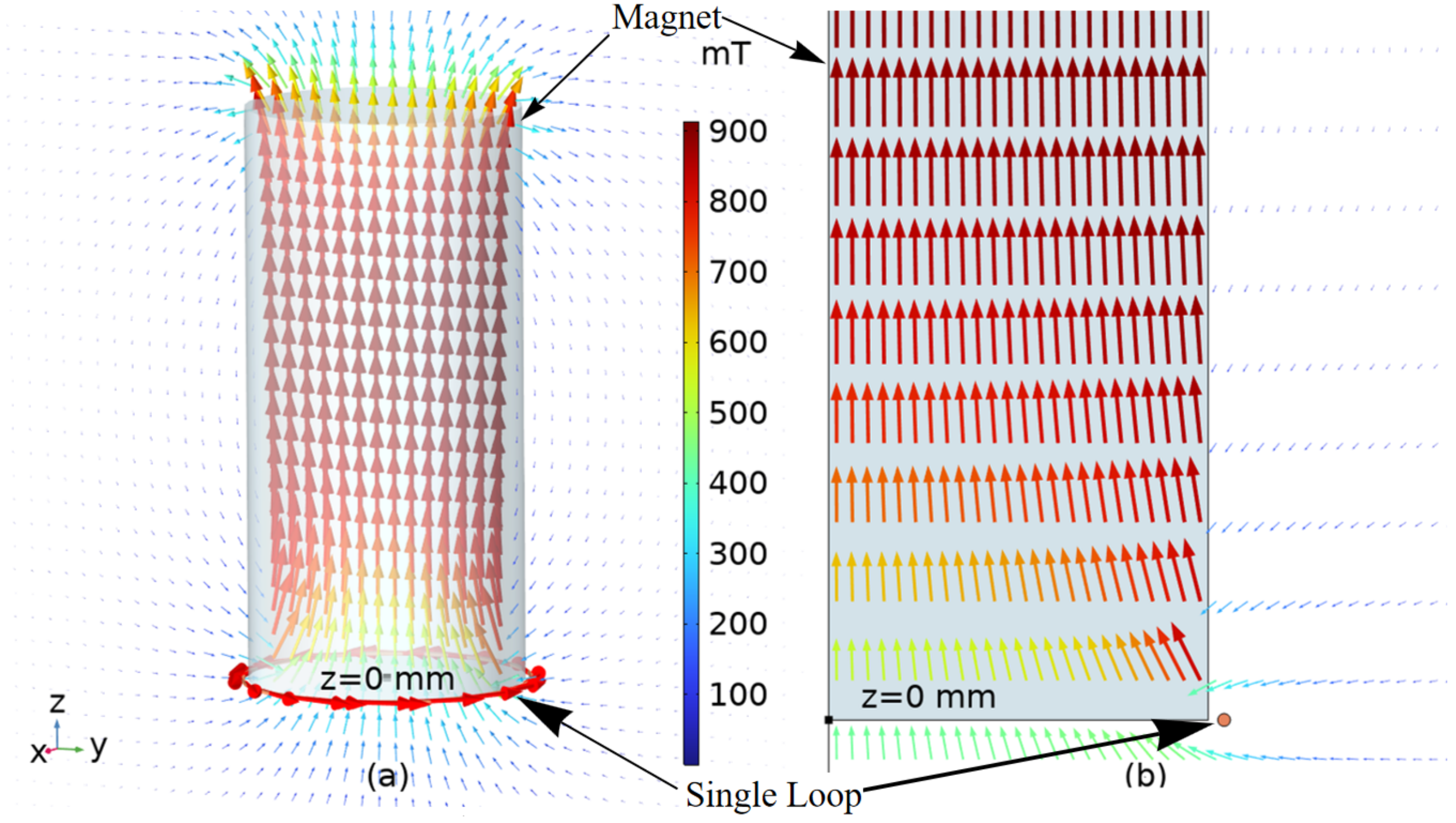
Figure 3 shows the COMSOL models of a single current loop with a radius of 5 mm in both 3D and axisymmetric 2D configurations. A DC current of 0.33 A flows through the loop, generating the magnetic field, B, as depicted in both models. In the 3D model, the current loop lies in the XY plane ($z=0$), with its center aligned with the origin of the Cartesian coordinate system. Based on the direction of the current density vector and the right-hand rule, the direction of the magnetic field on the YZ plane, as shown in the 3D model, is verified. Due to the symmetry of the 3D model about the Z-axis, it can be replaced by the axisymmetric 2D model shown in Figure 3.

The 2D model effectively captures all the key behaviors and properties of the underlying physics while significantly reducing computational memory requirements for a given mesh size, thanks to its lower dimensionality. To improve simulation accuracy, the maximum element size used in this study is set to 0.1 mm, and the discretization is configured as cubic instead of the default quadratic.

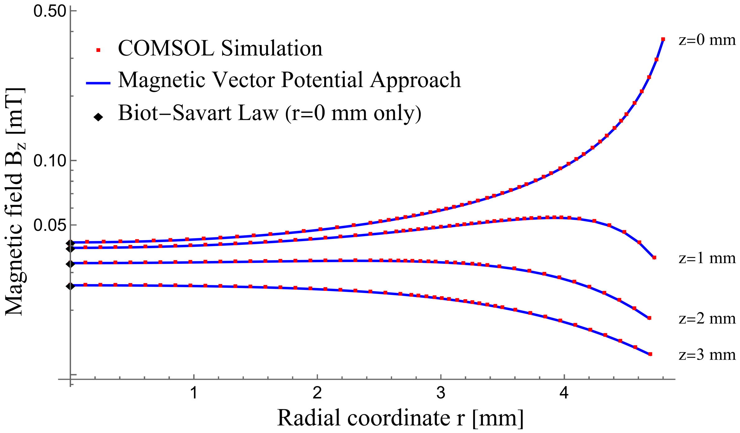
Figure 4 illustrates the axial component of the magnetic field magnitude ($B_z$) at four specific axial distances—$z=0$, 1, 2, and 3 mm from the XY plane—where the single loop is located. The plot shows the variation of the $B_z$ magnitude as a function of the loop’s radius and contains $B_z$ from COMSOL, the MVP approach, and the Biot–Savart law (just at the center) for the four aforementioned z levels. As shown, the COMSOL simulation and the MVP approach are in excellent agreement. Notably, along the axis of the coil, the results from the MVP approach and the Biot–Savart law align closely.

4.1.2. Axial Magnetic Field of a Multi-Loop Coil

In this section, we first model a random multi-loop coil using COMSOL. Figure 5 illustrates the 3D and 2D models of this coil. Specifically, the coil consists of 10 layers of AWG34 wire, with each layer containing 30 turns, resulting in a total of 300 turns. The inner radius of the coil is 5 mm, the outer radius is 6.6 mm, and its height is 4.8 mm. We then compared the $B_z$ from the theoretical model (MVP) with the results from the COMSOL simulations.

Similar to the single-loop case, we focus on the axisymmetric 2D model for the coil. In this model, a 0.33 A DC flows through the coil, generating a magnetic field around it. The direction of the magnetic field follows the right-hand rule.

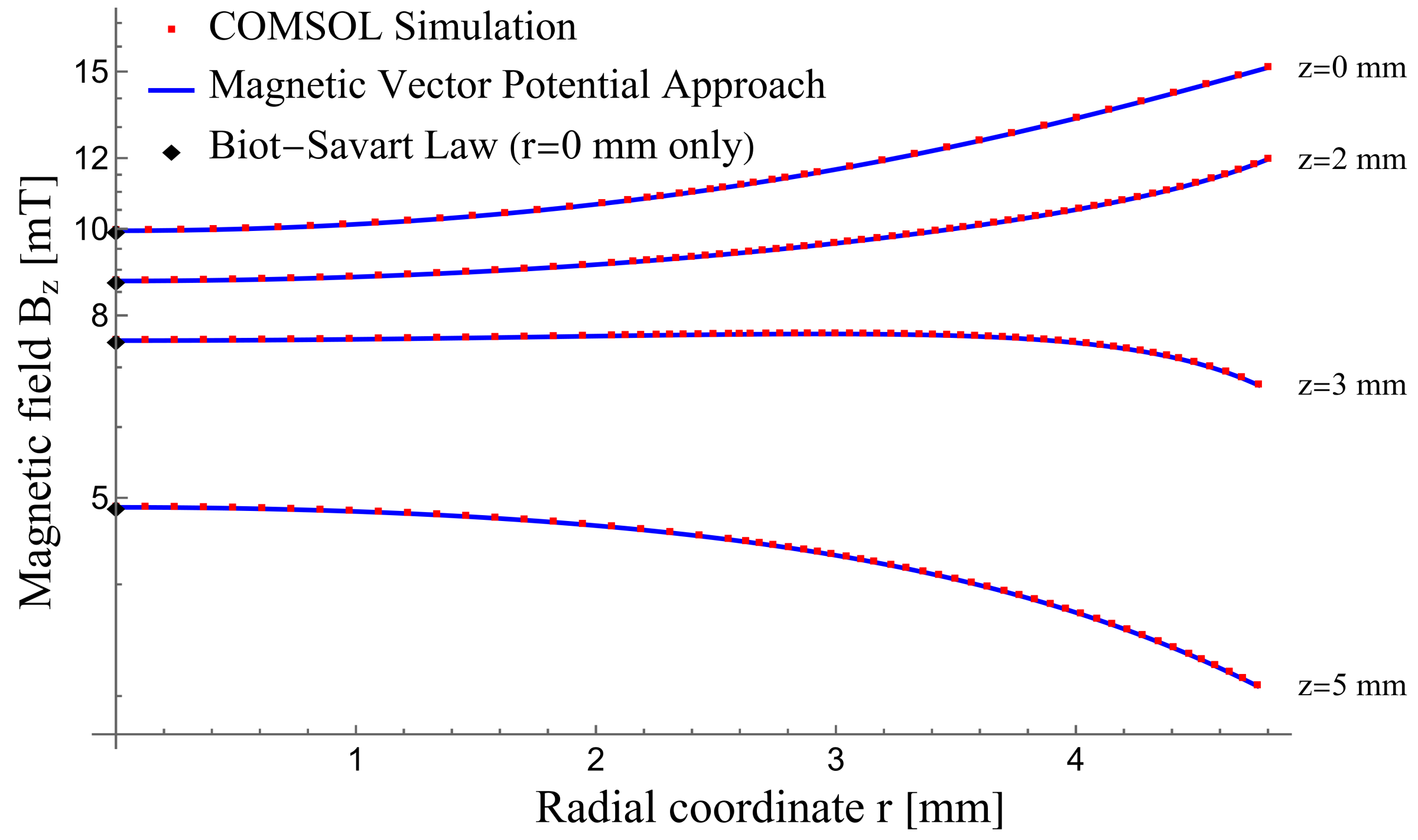
Figure 6 shows the axial component of the magnetic field magnitude ($B_z$) at four specific axial distances—$z=0$, 1, 2, and 3 mm from the XY plane—passing through the midpoint of the coil.

The results show excellent agreement between the COMSOL simulation and the theoretical MVP model. Similar to the previous case, along the axis of the coil, the results from the MVP approach closely align with those from the Biot–Savart law.

4.1.3. Force Generated by a Single Current-Carrying Coil

To investigate the force generated by a single current loop, we begin with the previously discussed single-loop case and then introduce a cylindrical permanent magnet into the model. The magnet has a diameter of 9.6 mm and a height of 20 mm. Its magnetization is defined using the remanent flux density ($B_r$), set to 1 T and oriented in the positive z-direction. Figure 7 shows the 3D and 2D models of this case.

Since COMSOL can compute the force exerted by the coil on the permanent magnet, we conducted a parametric sweep analysis by varying the vertical (z) position of the permanent magnet in 0.1 mm increments. The results are shown in Figure 8.

In Figure 8, the z-coordinate represents the position of the south pole of the permanent magnet. At $z=-10$ mm, since the coil is located exactly in the middle of the magnet, the forces from the south and north poles perfectly cancel each other, resulting in a net force of zero. At $z=0$ mm, the contribution from the south pole reaches its maximum, while the contribution from the north pole becomes negligible. At $z=10$ mm, the net force is significantly reduced due to the 10 mm separation between the south pole and the surface of the single current loop. The forces calculated using COMSOL and the MVP model show excellent agreement, as expected.

4.1.4. Force Generated by a Multi-Loop Current-Carrying Coil

By adding the same permanent magnet to the multi-loop coil, as shown in Figure 9, we can predict the force generated by the ESA based on its configuration.

For the multi-turn coil, we conducted a parametric sweep analysis by varying the vertical (z) position of the permanent magnet in 0.1 mm increments. Figure 10 shows the axial force exerted on the permanent magnet as a function of its position relative to the coil.

As anticipated, the force varies much less in the z-direction compared to the single-loop case. The agreement between the COMSOL simulation and the MVP approach validates that our model accurately predicts the force generated by the ESA. Compared to the COMSOL model, our method requires only a fraction of the computational power, time, and memory, making it highly suitable for parameter optimization.

4.2. Optimization Using MINLP

We conduct a set of simulations to demonstrate the optimization framework’s effectiveness in maximizing the $F/CSA$ of ESA. As detailed in Section 3.2, the optimization is performed using a mixed integer non-linear programming (MINLP) algorithm. For this analysis, the range for $N_{pl}$ was set between 26 and 80, while $d_m$ was varied between 5 mm and 15 mm. The total wire length was constrained to $L=10$ m.

After implementing the MINLP algorithm in MATLAB R2024a, we obtained the optimal design parameters for the ESA. The results indicate that the optimal values are $N_{pl}=53$, $d_m=7.91\mathrm{mm}$, and $N_l=6$. The total wire length used to form the coil is $L_{actual}=8.66\mathrm{m}$, with each wire having a diameter of 0.16 mm. The total number of turns in the coil is $N_{\mathrm{total}}=318$, calculated as $N_{\mathrm{total}}=N_{pl}·N_l$. The length of the coil is $N_{pl}·d_w\mathrm{mm}=8.48\mathrm{mm}$, and the outer diameter of the coil is determined as $d_i+(N_l·d_w)=9.26\mathrm{mm}$. The resulting maximum force per unit cross-sectional area is $F/CSA=5.74{\mathrm{mN}/\mathrm{mm}}^2$.

To validate the optimization results, these parameters were then used to model the same actuator in COMSOL Multiphysics, where we simulated and obtained the F/CSA. The COMSOL result was $5.71{\mathrm{mN}/\mathrm{mm}}^2$, closely matching the optimized value of $5.74{\mathrm{mN}/\mathrm{mm}}^2$. This strong correlation confirms the accuracy and reliability of the proposed optimization method.

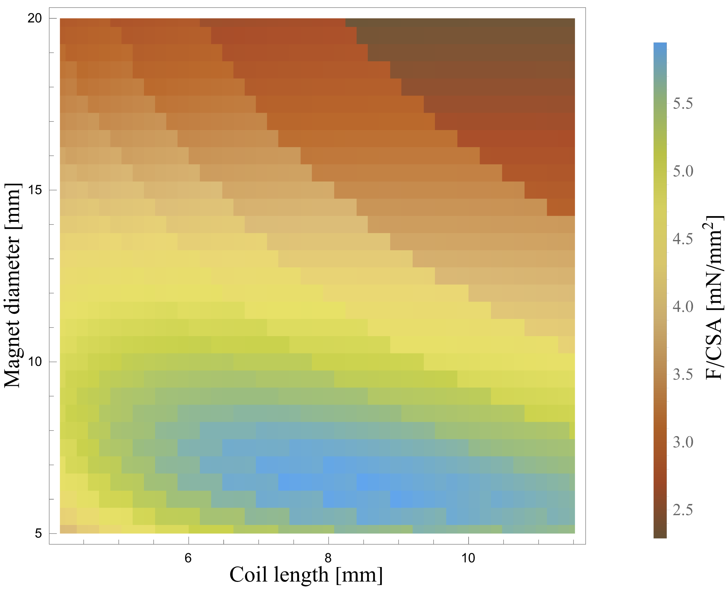
Additionally, a parametric sweep of the F/CSA results from the analytical MVP approach was conducted by varying two variables: the number of turns per layer ($N_{pl}$) and the diameter of the permanent magnet ($d_m$). The results of this sweep are presented in Figure 11. The optimized values from the MINLP algorithm are located within the blue region of these plots, indicating they lie within the high-performance region. This additional validation highlights the consistency and precision of the optimization approach.

5. Conclusions

In this work, we employed the analytical magnetic vector potential (MVP) approach to accurately calculate the magnetic field and generated force of an electromagnetic soft actuator (ESA). Additionally, we introduced a mixed integer non-linear programming (MINLP) optimization framework to maximize the (F/CSA) by jointly optimizing key design parameters, such as the number of turns per layer ($N_{pl}$) and the permanent magnet diameter ($d_m$). COMSOL simulations confirmed the consistency between MVP-based calculations and physical simulations. Furthermore, the results demonstrated the effectiveness of the MINLP optimization framework in identifying optimal design configurations that significantly enhance the F/CSA.

Minimizing the size of ESAs is crucial for developing compact actuator networks that can function as soft muscles in constrained spaces, enabling applications in rehabilitation and assistive technologies. Beyond soft robotics, our developed model also facilitates optimization in broader applications involving the interaction between a permanent magnet and an adjacent circular coil. This includes technologies such as electric motors and other electromagnetic systems, where similar components are essential for improving performance and efficiency. Notably, within these systems, the MVP approach proves valuable in non-destructive evaluation (NDE) techniques that operate within the quasi-DC regime, where displacement current can be neglected, even at high frequencies. In such applications, including eddy current testing (ECT) and electromagnetic acoustic transducers (EMATs), the analytical MVP approach can be used to accurately calculate the magnetic field and Lorentz force, enabling precise evaluations of system performance and material integrity.

Compared to finite element-based COMSOL simulations, the analytical MVP approach offers significant advantages in computational efficiency, requiring considerably less memory and CPU time while maintaining high accuracy. Unlike finite element simulators that require discretization of the entire computational domain—that is, volume in 3D and area in 2D—the MVP approach relies on mathematical expressions that can be evaluated with minimal computational cost. These advantages make the MVP approach not only a powerful tool for model validation but also an effective solution for design optimization, data visualization, and parametric analysis in a variety of applications, including those in electromagnetic system design and evaluation.