Article

Inverse System Decoupling Control of Composite Cage Rotor Bearingless Induction Motor Based on Support Vector Machine Optimized by Improved Simulated Annealing-Genetic Algorithm

1
School of Electrical and Photoelectric Engineering, West Anhui University, Lu’an 237012, China
2
School of Electrical and Information Engineering, Jiangsu University, Zhenjiang 212013, China
3
School of Electronics and Information Engineering, West Anhui University, Lu’an 237012, China
*
Author to whom correspondence should be addressed.
Actuators 2025, 14(3), 125; https://doi.org/10.3390/act14030125
Submission received: 5 January 2025 / Revised: 1 March 2025 / Accepted: 4 March 2025 / Published: 5 March 2025
(This article belongs to the Section Control Systems)

Abstract

:
To address the inherent nonlinearity and strong coupling among rotor displacement, speed, and flux linkage in the composite cage rotor bearingless induction motor (CCR-BIM), an inverse system decoupling control strategy based on a support vector machine (SVM) optimized by the improved simulated annealing-genetic algorithm (ISA-GA) is proposed. First, based on the structure and working principle of CCR-BIM, the mathematical model of CCR-BIM is derived, and its reversibility is rigorously analyzed. Subsequently, an SVM regression equation is established, and the SVM kernel function parameters are optimized using the ISA-GA to train a high-precision inverse system decoupling control model. Finally, the inverse system is cascaded with the original system to construct a pseudo-linear system model, achieving linearization and decoupling control of CCR-BIM. To verify the effectiveness and practicability of the proposed decoupling control strategy, the proposed control method is compared with the traditional inverse system decoupling control strategy through simulation and experimentation. Both simulation and experimental results demonstrate that the proposed decoupling control strategy can effectively achieve decoupling control of rotor displacement, rotational speed, and flux linkage in CCR-BIM.

1. Introduction

The induction motor (IM) exhibits numerous advantages, such as a simple structure, reliable operation, excellent starting performance, high efficiency, high starting torque, and flexible speed control. Consequently, it has been widely applied in various fields, including industrial drives, transportation, wind power generation, mining machinery, and aerospace applications [1,2,3,4]. Traditional IMs utilize mechanical bearings to support their rotating shafts, which is a common design in conventional motor systems. However, as the rotational speed increases, significant friction and wear are generated, leading to reduced lifespan and system reliability [5,6]. To address this issue, a composite cage rotor bearingless induction motor (CCR-BIM) has been proposed [7,8]. Compared to traditional IM, CCR-BIM offers advantages such as the elimination of friction and wear, no lubrication requirements, and prolonged service life. Consequently, the CCR-BIM holds significant potential for application in specialized environments, including cleanrooms, corrosive conditions, and vacuum systems.
However, CCR-BIM is a multivariable, nonlinear, and strongly coupled system. During the operation of the motor, there is a strong coupling relationship between rotor displacement, speed, and magnetic flux. Therefore, a control strategy needs to be designed to achieve decoupling control of CCR-BIM. The key to precise control of CCR-BIM lies in linearizing its nonlinear system, thereby enabling the application of a linear controller for dynamic decoupling control. Inverse system linearization, as an effective method for nonlinear-to-linear transformation, can decouple the original system into multiple pseudo-linear subsystems. Moreover, the support vector machine (SVM) exhibits excellent nonlinear modeling and generalization capabilities, even with small sample sizes [9,10,11,12].
By utilizing the support vector machine (SVM) to approximate the inverse system of CCR-BIM, the controlled object can be compensated to behave as a linear and decoupled pseudo-linear system. The work in [13] introduces a novel decoupling control method that utilizes the inverse of the Least Squares Support Vector Machine (LS-SVM) for Bearingless Synchronous Reluctance Motors (BSRMs). An offline LS-SVM inverse model is constructed to decouple the BSRMs into three single-input, single-output pseudo-linear systems. The work in [14] introduces an innovative approach that employs LS-SVM and an inverse system to establish a decoupling model for the control of driving current and radial force current in a Single-Winding Bearingless Switched Reluctance Motor (SWBSRM). The proposed methodology is rigorously validated through simulations based on an Internal Model Control (IMC) framework. The work in [15] presents an innovative decoupling control strategy for the bearingless synchronous reluctance motor. This method harnesses the strengths of LS-SVM in small sample learning, universal approximation, and identification fitting to derive inverse models of the motor. By integrating these LS-SVM inverse models with the original system in a cascaded manner, the intricate nonlinear multivariable system is decoupled into three single-input, single-output (SISO) pseudo-linear subsystems. Based on the principles of linear control theory, closed-loop controllers are subsequently designed for these decoupled subsystems. The work in [16] introduces an innovative control approach tailored for the bearingless induction motor. This strategy utilizes the LS-SVM first-order inverse system method to accomplish dynamic decoupling control between torque and suspension force. By integrating the inverse system, which is identified through LS-SVM, with the original system in a cascaded configuration, the inherently nonlinear bearingless induction motor system is decoupled into four autonomous pseudo-linear subsystems. Subsequently, linear control system techniques are employed to synthesize and simulate these decoupled subsystems. The research findings demonstrate that this control strategy effectively achieves dynamic decoupling control between torque and suspension forces within the bearingless induction motor.
The decoupling control algorithms proposed in references [13,14,15,16] can achieve inverse decoupling control of various motors, but it does not optimize the performance parameters of support vector machines (SVM), leaving room for further improvement of decoupling accuracy. In this article, a support vector machine (SVM) is employed to identify the inverse system of the CCR-BIM to achieve decoupling control. To enhance the accuracy of the SVM in identifying the inverse system, an improved simulated annealing-genetic algorithm (ISA-GA) is proposed to optimize the SVM kernel function, thereby improving search efficiency and local optimization capabilities, and augmenting the SVM’s ability to identify the inverse system of CCR-BIM. Utilizing the optimized SVM, the inverse system is constructed and cascaded with the original system to form a pseudo-linear system, enabling linearization and decoupling control of the CCR-BIM. The feasibility and effectiveness of this approach are verified through simulations and experiments presented.

2. Suspension Mechanism, Topology, and Mathematical Model of CCR-BIM

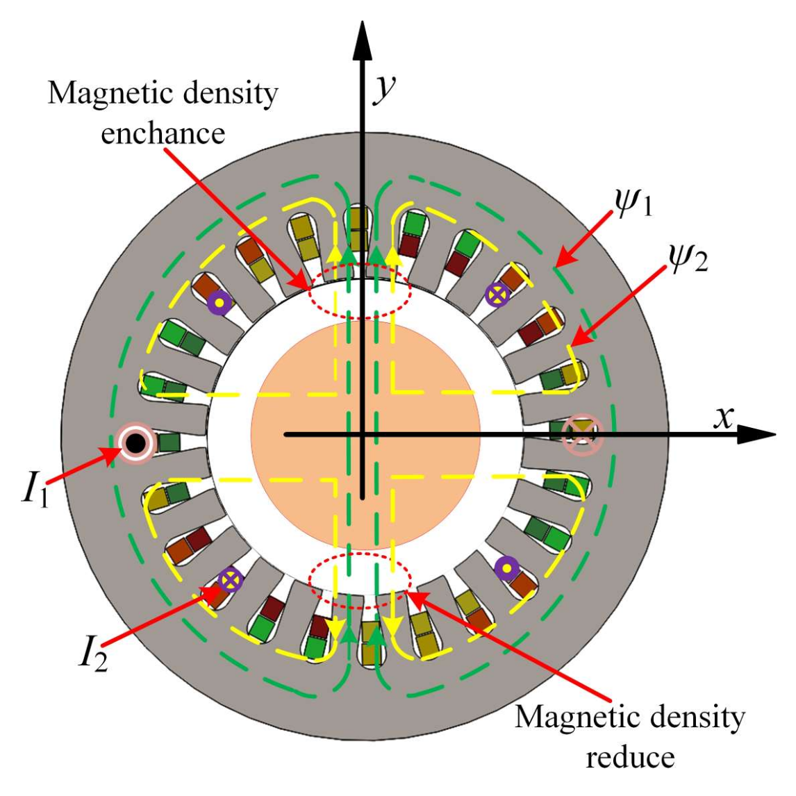
2.1. Suspension Mechanism of CCR-BIM

Compared to IM, the stator of CCR-BIM features two windings: the torque winding and the suspension force winding. The pole pairs of the torque winding and the suspension winding are marked as P1 and P2, respectively. When the condition P1 = P2 ± 1 is satisfied between them, and the electrical angular frequencies of the two windings are equal (dj1 = dj2), an interaction between the magnetic fields generated by the windings with different pole pairs produces controllable radial forces. This interaction enables the stable suspension of the CCR-BIM rotor. The mechanism for generating radial forces is illustrated in Figure 1 [17,18,19,20].

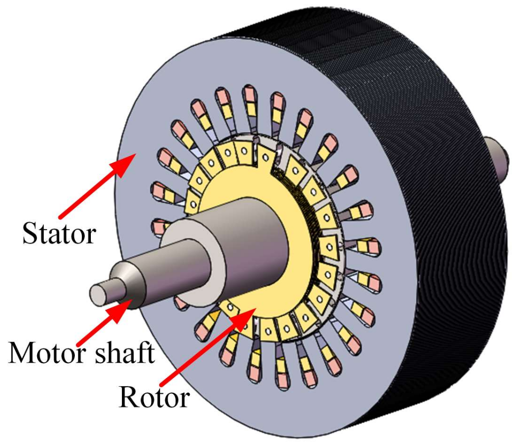
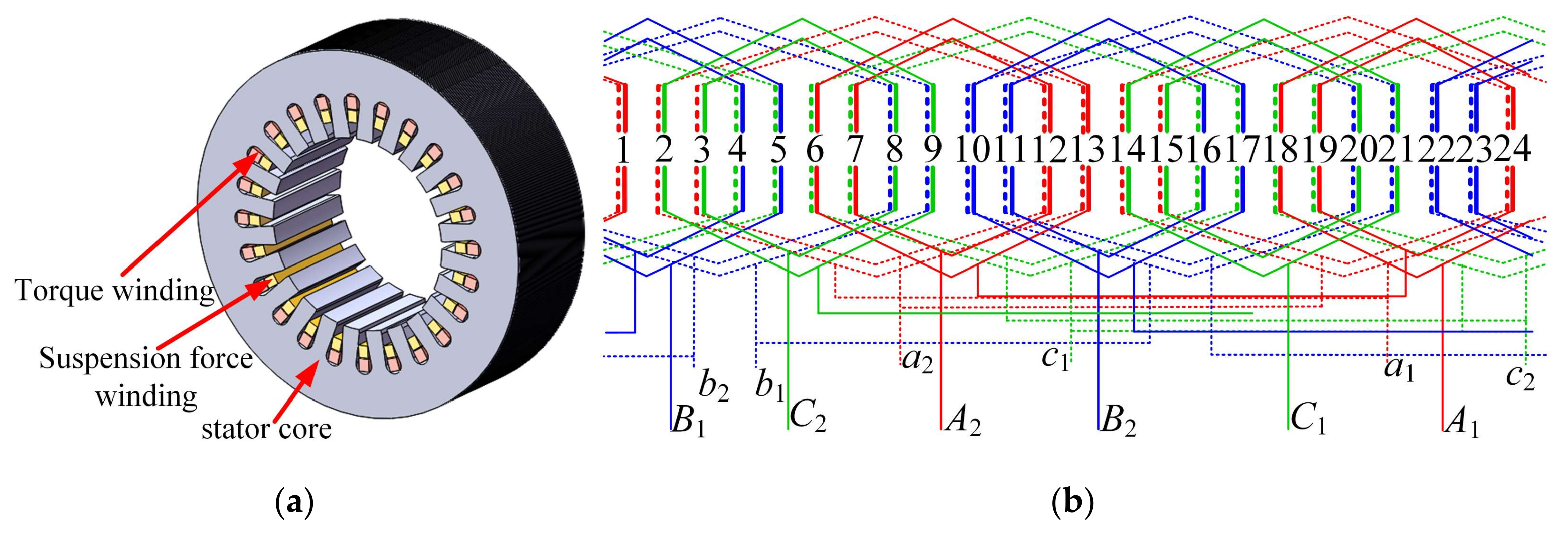
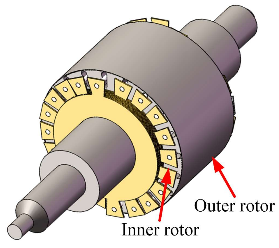
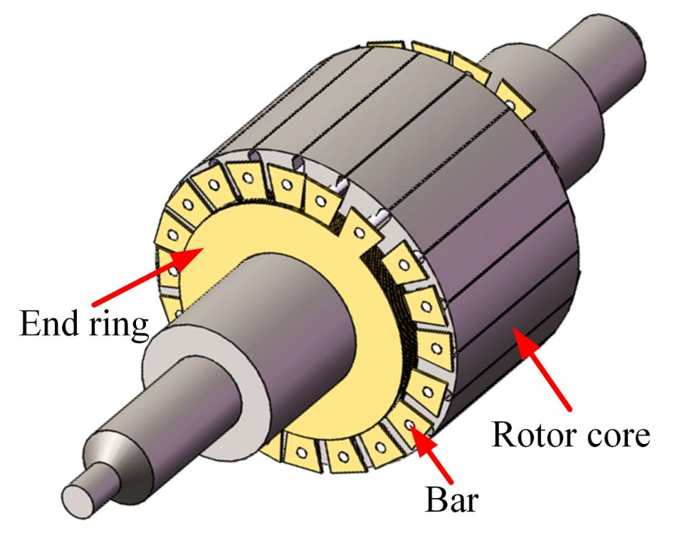
2.2. Topology of CCR-BIM

The CCR-BIM inherits the structural composition of traditional IM in its topological design, primarily consisting of stator, rotor, and shaft. The topology of CCR-BIM is illustrated in Figure 2.
In the CCR-BIM, the stator comprises a stator core and two windings. The stator core slots are embedded with two sets of windings: the torque winding and the suspension force winding. The torque winding provides the driving torque for the composite cage rotor and has a pole pair number of 1, i.e., P1 = 1. The suspension force winding generates sufficient radial force on the composite cage rotor to maintain stable self-suspension of the rotor and has a pole pair number of 2, i.e., P2 = 2. The stator core is composed of 0.5 mm thick silicon steel laminations and fasteners. In the prototype design presented in this article, the stator core has 24 slots. The torque winding is placed at the bottom of the stator core slots, and the suspension force winding is placed at the top of the slots. The structural model of the stator is illustrated in Figure 3a. In the CCR-BIM stator, both windings are arranged in a single-layer concentric distribution. Two separate inverter power supply units power the torque winding and the suspension force winding. Figure 3b shows the distribution of the torque winding and the suspension force winding. The dashed lines represent the distribution of the torque winding, with terminals labeled as a1 and a2, b1 and b2, c1 and c2, respectively. Based on the winding configuration, the torque winding has one pole pair. The solid lines represent the distribution of the suspension force winding, with terminals labeled as A1 and A2, B1 and B2, C1 and C2, respectively. The winding configuration confirms that the number of pole pairs for the suspension force winding is 2.
The rotor of CCR-BIM features a specially designed composite cage structure, consisting of an outer rotor and an inner rotor, as illustrated in Figure 4. The outer rotor consists of a solid layer made of high-permeability silicon steel. Due to the skin effect, the solid structure made of high-permeability silicon steel concentrates the current on its surface, enabling the composite cage rotor to achieve a higher starting torque. This allows the motor to overcome greater resistance during the startup process.
The inner rotor is composed of the rotor core, specially designed bar assemblies, and the end rings. The structure of the inner rotor is illustrated in Figure 5. In the prototype design presented in this paper, the rotor core is constructed by laminating 0.5 mm silicon steel sheets, with 20 slots machined into the rotor core. The bars are made of aluminum and have a radius of 3.5 mm. The end rings are fabricated from copper, offering excellent electrical conductivity and thermal resistance.
The special bar assembly structure of the inner rotor’s squirrel-cage configuration is illustrated in Figure 6a, where each individual bar assembly consists of two symmetrical bars and two end rings at the beginning and end, forming a unique closed-loop bar structure. Given that the inner rotor core is provided with 20 slots, with each set of bar assemblies installed in every two symmetrical slots, a total of 10 sets of bar assemblies are required to fill the slots of the inner rotor core. Figure 6b shows the resulting squirrel-cage bar assembly structure, which is achieved by arranging and installing the bar assemblies sequentially according to a specific pattern.
The induction mechanism of the special squirrel-cage structure is as follows. Within the motor’s magnetic field, which is constructed by the three-phase symmetrical windings of the CCR-BIM, the magnetomotive force (MMF) describes the distribution of the magnetic field in both time and space. The MMF f(x,t) at any circumferential position x of the squirrel-cage rotor can be expressed as [21]:
f ( x , t ) = F cos ( ω t P x )
where F represents the amplitude of the fundamental MMF, and ω represents the angular velocity of the rotating magnetic field.
The analysis focuses exclusively on the distribution of bar currents when only the torque winding and the suspension force winding are energized. Arbitrarily select a point x1 on the circumference of the squirrel-cage structure, with its symmetric position on the circumference marked as x2. Assuming the pole pair number of the torque winding P1 = 1 and the pole pair number of the suspension force winding P2 = 2, the mathematical expression for the MMF can be represented as:
f 1 ( x 2 , t ) = F 1 cos ( ω t x 2 ) = f 1 ( x 1 , t ) , P 1 = 1 f 2 ( x 2 , t ) = F 2 cos ( ω t 2 x 2 ) = f 1 ( x 1 , t ) , P 2 = 2
By analyzing Equation (2), the distribution of induced currents in the bars is illustrated in Figure 7. Within the magnetic field of the torque winding, the induced electromotive forces (EMFs) at points x1 and x2 are in opposite directions, resulting in the formation of a closed current loop within a specific individual bar set. Thus, the torque winding can induce currents in the special squirrel-cage rotor. Conversely, in the magnetic field of the suspension force winding, the EMFs at points x1 and x2 are in the same direction, causing the currents in the enclosed individual bar set to cancel each other out, resulting in a total current of zero. Therefore, the suspension force winding cannot induce currents in the special squirrel-cage rotor.
It is demonstrated that only the induced current generated by the torque winding exists in the specially designed squirrel-cage bars, while the induced current produced by the suspension force winding is canceled out. Consequently, the specially designed squirrel-cage rotor only senses the torque winding, meaning that only the torque winding needs to be considered in the torque mathematical model. Furthermore, the induction of the suspension force winding on the special squirrel-cage rotor is effectively shielded, which enhances the control accuracy of the torque winding.

2.3. Mathematical Model of CCR-BIM

The mathematical model for the suspension force in CCR-BIM is expressed as [8]:
F x F y = B 1 M B 2 M π r l 2 μ 0 cos ( λ ) sin ( λ )
where Fx and Fy represent the resultant force components of the radial forces in the x-axis and y-axis directions, respectively, B1M and B2M represent the electromagnetic inductions of the torque winding and suspension force winding, respectively, r represents the rotor radius, l is the effective length of the rotor, μ0 represents the air permeability, λ is the difference between the initial angle of torque winding current and suspension winding current.
T e = L 1 m ( i 1 d r i 1 q s i 1 d s i 1 q r ) = i 1 q s ψ 1 d i 1 d s ψ 1 q
where ψ 1 d and ψ 1 q represent the air gap flux components along the d-axis and q-axis of the torque winding, respectively, L1m is the self-inductance of the torque winding, i1dr and i1qr represent the rotor current components of the d-axis and q-axis of the torque winding, respectively, i1dsand i1qs represent the stator current components of the d-axis and q-axis of the torque winding, respectively.
The expression for the torque motion equation is:
T e T L = J P 1 d ω ˙ r d t
where TL represents the load torque, and J represents the moment of inertia.

3. Establishment of SVM Inverse System Optimized by ISA-GA

3.1. Reversibility Analysis of CCR-BIM

Based on the inverse system theory, the output variables, state variables, and input variables of the CCR-BIM system are defined as follows:
The output variables are defined as Z = x , y , ω r , ψ , the state variables are defined as V = [ x , y , x ˙ , y ˙ , ω r , ψ 1 r d , ψ 1 r q ] T , the input variables are defined as U = [ i 2 s d , i 2 s q , i 1 r d , i 1 r q ] T , where x and y represent the suspension displacement parameters; 1 represents the torque winding parameter, 2 represents the suspension force winding parameter, s represents the stator parameter, r represents the rotor parameter, d represents the d-axis parameter, and q represents the q-axis parameter.
The state equation of the CCR-BIM can be expressed as:
z ˙ 1 = v ˙ 1 = v 3 z ¨ 1 = v ¨ 1 = v ˙ 3 = K u 1 u 3 K u 2 u 4 + f v / m z ˙ 2 = v ˙ 2 = v 4 z ¨ 2 = v ¨ 2 = v ˙ 4 = ( K u 1 u 4 + K u 2 u 3 f v ) / m z ˙ 3 = v ˙ 5 = ( L 1 m P 2 2 v 6 u 2 L 1 m P 2 2 v 7 u 1 P 1 T L L r ) / J L r z ˙ 4 = ( L 1 m u 2 + L 1 m u 1 v 6 2 v 7 2 ) / T r v 6 2 + v 7 2
By taking the partial derivatives of the input variables U in Equation (6), the Jacobian matrix can be obtained as follows:
A = z ¨ 1 , z ¨ 2 , z ˙ 3 , z ˙ 4 U = K m u 3 u 4 u 1 u 2 u 4 u 3 u 2 u 1 m J K P 2 2 L 1 m v 7 m J K P 2 2 L 1 m v 6 0 0 m K v 6 v 6 2 + v 7 2 L 1 m T r m K v 7 v 6 2 + v 7 2 L 1 m T r 0 0
According to Equation (7), it can be deduced that the determinant of the Jacobian matrix A is not equal to zero, and the corresponding relative degree of the system is α = [ α 1 , α 2 , α 3 , α 4 ] = [ 2 , 2 , 1 , 1 ] , which satisfies the condition α 1 + α 2 + α 3 + α 4 6 . Therefore, the system meets the reversibility criteria for an inverse system.
The inverse system representation of the state equation for the CCR-BIM system is given by:
U = u 1 , u 2 , u 3 , u 4 T = ξ ¯ z 1 , z ˙ 1 , z ¨ 1 , z ˙ 2 , z ˙ 2 , z ¨ 2 , z ˙ 3 , z ˙ 4 , z 4 T
The system model in Equation (7) possesses reversibility, which fulfills the fundamental condition for achieving decoupling control of CCR-BIM. However, in practical control system applications, the complexity of the CCR-BIM state equation is too high for conventional analytical methods to accurately derive its regression model. To realize decoupling control using the inverse system of CCR-BIM, it is necessary to employ SVM to construct a more precise and effective inverse system model for CCR-BIM.

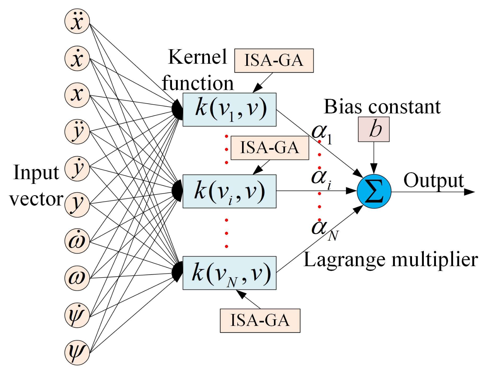
3.2. Establishment of SVM Model

In an n-dimensional space, the expression for the geometric margin between a point and a hyperplane is given by:
d = y ω , v + b ω
where ω = ω 1 2 + + ω n 2 , y i ω , v + b 1 (i = 1, 2, 3, ⋯, n). It can be observed that the scaling of ω and b has a minor impact on the geometric margin. Therefore, we can set dmin = 1. Additionally, the process of solving for max 1 ω is transformed into computing. Hence, the following is the process for solving the min 1 2 ω 2 minimization problem [22,23,24]:
min 1 2 ω 2 s . t .   z i ω , v i + b = d i 1   i = 1 , 2 , , n
Transforming the original problem into a convex quadratic programming problem under linear constraints is achieved through the above process. To solve this problem, a Lagrange function incorporating n training samples is constructed:
L ω , b , α = 1 2 ω 2 i = 1 n α i z i ω , v i + b 1
To ensure that the Lagrange function satisfies the constraint conditions while achieving the maximum value, the parameters are restricted to αi ≥ 0. The objective function expression at this point is:
min ω , b   max α ι 0   L ω , b , α
Equation (11) has a saddle point that satisfies the stationarity, feasibility, and complementary slackness conditions within the Karush–Kuhn–Tucker (KKT) framework. Consequently, Equation (12) can be equivalently transformed into solving a set of dual problems, specifically expressed as:
max α ι 0   min ω , b   L ω , b , α
By fixing the parameter α, the partial derivatives of ω and b are taken to find the minimum value of Equation (11) regarding ω and b. The mathematical expression is:
L ω = ω i = 1 n α i z i v i = 0 L b = i = 1 n α i z i = 0
Substituting Equation (14) into the Lagrange function shown in Equation (11) yields:
L ω , b , α = 1 2 ω 2 i = 1 n α i z i ω , v + b 1 = 1 2 ω T i = 1 n α i z i v i ω T i = 1 n α i z i v i b 0 + i = 1 n α i = i = 1 n α i 1 2 i = 1 n α i z i v i T i = 1 n α i z i v i = i = 1 n α i 1 2 i , j = 1 n α i α j z i z j v i T v j
The objective function in the original Equation (13) is transformed into:
max α i = 1 n α i 1 2 i , j = 1 n α i α j z i z j v i , v j s . t .   α i 0 , i = 1 , 2 , , n   i = 1 n α i z i = 0
Using the Sequential Minimal Optimization (SMO) recursive method to calculate the Lagrange multipliers α, and subsequently calculating ω and b, the maximum margin hyperplane can be determined. The classification function can be expressed as:
f ( v ) = i = 1 n α i z i v i T v + b = i = 1 n α i z i v i , v + b
Figure 8 illustrates the analysis process for nonlinear sample processing. Specifically, when outliers are in the state shown in Figure 8a, the sample points become linearly inseparable. Data measurement errors or noise introduces outliers, which inevitably affect the margin of the maximum margin hyperplane. This situation can be effectively improved by introducing a loss function, whose expression is as follows:
E = i = 1 n e i 2 = i = 1 n 1 z i ω , v + b 2
To ensure that the maximum margin hyperplane meets the constraint conditions at any position, corresponding constraints need to be applied to the deviation. Here, the deviation is squared and then added cumulatively to the objective function. The adjusted optimization objective for the objective function in Equation (10) is:
min 1 2 ω 2 + 1 2 γ i = 1 n e i 2 s . t .   z i ω , v i + b + e i = 1 ,   i = 1 , 2 , , n
where γ is the parameter controlling the weight.
Equation (19) calculates the sum of squares of deviations, and after corresponding adjustments, the Lagrange function is expressed as:
L ( ω , b , e , α ) = 1 2 ω 2 + 1 2 γ i = 1 n e i 2 i = 1 n α i y i ω , v i + b + e i 1
The corresponding objective function is represented as follows:
min ω , b , e , α   L ( ω , b , e , α )
Equation (20) is the optimized Lagrange function, and it can be observed that the original problem has been transformed into solving a system of linear equations after processing.
Figure 8b illustrates a scenario where the two types of samples cannot be separated within the sample space, i.e., the sample points themselves are in a nonlinear state. The solution involves mapping the sample to a higher-dimensional space, as depicted in Figure 8c. The nonlinear sample classification process mainly consists of two stages. First, the sample is mapped to a higher-dimensional feature space, and then a linear learning machine is used for classification in this high-dimensional space.
The specific process is as follows. In a two-dimensional space, the coordinates can be represented as (v1, v2), and any curve equation can be written as:
a 1 v 1 2 + a 2 v 2 2 + a 3 v 1 v 2 + a 4 v 1 + a 5 v 2 + a 6 = 0
Taking a five-dimensional space as an example, let w 1 = v 1 2 , w 2 = v 2 2 , w 3 = v 1 v 2 , w 4 = v 1 , w 5 = v 2 , then the curve equation in the two-dimensional space can be expressed as:
i = 1 5 a i w i + a 6 = 0
Therefore, in the newly constructed coordinate system, by introducing a hyperplane equation, the sample points that were originally linearly inseparable in the low-dimensional space can be linearly separated in the high-dimensional space. The classification function at this time can be reformulated as:
f ( v ) = i = 1 n α i z i λ v i , λ v + b
When the number of input features for SVM is 2, the hyperplane appears as a straight line. When the number of input features increases to 3, the hyperplane becomes a two-dimensional plane. However, when the number of features exceeds 3, the mapped dimensions will increase significantly, leading to a dimensionality explosion. To avoid this, a kernel function k is introduced. Introducing the kernel function allows the samples to be implicitly mapped to a high-dimensional space without explicitly computing the coordinates of the mapped samples. This approach effectively avoids the dimensionality explosion problem while achieving computation results equivalent to those obtained through explicit high-dimensional mapping.
The specific expression of the kernel function k is as follows:
k ( v 1 , v 2 ) = χ v 1 , v 2 = λ v 1 , λ v 2
After dimensionality reduction using the kernel function, the classification function corresponding to Equation (24) can be rewritten as:
f ( v ) = i = 1 n α i z i k ( v i , v ) + b
From the above analysis, it can be seen that SVM has the ability to fit any nonlinear function. The following function fitting result can be obtained:
z ^ i = ω T λ ( v i ) + b , i = 1 , , n
The constraint condition in the above equation is:
z i = ω T λ ( v i ) + b + e i , i = 1 , , n
where zi is the actual output corresponding to vi.
The optimization objective is transformed to:
min 1 2 ω 2 + 1 2 γ i = 1 n e i 2 s . t .   z i = ω T λ ( v i ) + b + e i , i = 1 , , n
Based on Equations (27) and (28), the Lagrange equation is constructed as:
L ( ω , b , e , α ) = 1 2 ω 2 + 1 2 γ i = 1 n e i 2   i = 1 n α i ( ω T λ ( v i ) + b + e i z i )
According to the KKT conditions, the partial differential equation of the above equation is obtained, with the specific expression as follows:
L ω = ω Σ n i = 1 α i λ ( v i ) = 0 L b = Σ n i = 1 α i = 0 L e i = γ e i α i = 0 L α i = ω T λ ( v i ) + b + e i z i = 0   ω = Σ n i = 1 α i λ ( v i ) e i = α i γ Σ n i = 1 α i = 0 z i = ω T λ ( v i ) + b + e i
Solving Equation (31) yields:
0 I n T I n Ω + γ 1 I n b α = 0 z
where Ω is the diagonal matrix of the kernel function, with diagonal elements as k ( v i , v ) ,   i = 1 , 2 , , n ; z = [ z 1 , , z n ] T , and In is the identity matrix.
By selecting a kernel function, the SVM regression equation is obtained as:
z ( v ) = i = 1 n α i k ( v i , v ) + b
The fitting process of the SVM regression equation in Equation (33) heavily relies on the kernel function of the SVM. Therefore, the selection of the kernel width of the kernel function is crucial, as an appropriate kernel width can effectively improve the prediction accuracy of the model. Thus, the ISA-GA is employed to determine the optimal kernel width.

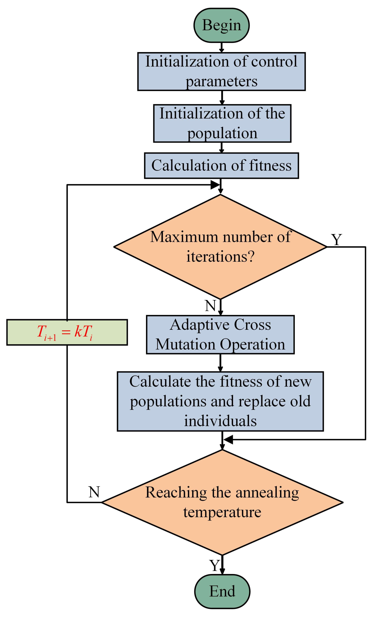
3.3. Optimal Design of Kernel Function Based on ISA-GA

By leveraging the global search capability of genetic algorithms and the local search capability of simulated annealing algorithms, the simulated annealing-genetic algorithm (SA-GA) demonstrates robust performance in solving complex optimization problems. The SA-GA employs two fundamental operations: genetic operations and simulated annealing operations, where genetic operations constitute the global search component of the genetic simulated annealing algorithm. However, genetic algorithms exhibit limitations in local search, often leading to premature convergence to local optimal solutions. Traditional genetic algorithms typically utilize fixed crossover and mutation operators, and despite numerous experimental adjustments to these parameters, it remains challenging to ensure their optimality in every instance. Consequently, this to some extent affects the efficiency and accuracy of the algorithm in finding optimal solutions [25,26]. In light of this, it is necessary to improve the crossover and mutation operators of genetic algorithms to enhance their global search capability.
The parameter optimization process for the improved simulated annealing-genetic algorithm (ISA-GA) supporting the SVM is as follows:
(1)
Initialization of Population: Initialize the population by randomly generating individuals, each representing a potential solution.
(2)
Genetic Operations: Evolve the population using selection, adaptive crossover, and mutation operations to update the fitness of each individual.
(3)
Simulated Annealing Operations: Apply simulated annealing to each individual to conduct a local search for better solutions.
(4)
Stopping Condition Check: Check if the preset stopping conditions for iteration have been met.
(5)
Return Optimal Solution: Return the optimal individual as the final result.
The genetic operations in genetic algorithms are of crucial importance. The primary processes include selection, crossover, and mutation. The selection operation involves choosing the more superior individuals from the old population to form a new population. There are numerous methods for this selection, and in this design, the roulette wheel selection method is employed, with its specific expression given below:
P i = f i k = 1 M f k
where fi represents the fitness of individual i, and M denotes the population size.
This article introduces an adaptive crossover and mutation strategy that dynamically adjusts parameter values at different stages of population evolution to better suit the evolutionary needs of each generation. When there is a significant difference between the current population’s average fitness and the optimal fitness, it indicates a high degree of dispersion and rich diversity within the population. Based on the fundamental principles of genetic algorithms, it is recommended to increase the crossover operator’s value to facilitate more thorough crossover operations within the population, thereby generating more competitive individuals. Meanwhile, to protect high-quality individuals, the mutation operator’s value should be moderately decreased to reduce potential interference with advantageous genes, thereby accelerating the overall convergence speed of the algorithm. Consequently, when the aforementioned difference is small, the crossover operator’s value should be reduced accordingly. The process of constructing the expressions for the adaptive crossover operator and adaptive mutation operator is as follows.
The expression for the adaptive crossover operator with an adaptive coefficient kc is set as:
P c = k c × f a v g f max , f a v g f max < 0.5 k c × ( 1 f a v g f max ) , f a v g f max 0.5
where f a v g represents the average fitness value, f max represents the maximum fitness value, and f a v g f max is used to measure the current population dispersion.
The expression for setting the mutation operator value with an adaptive coefficient k m is given by
P m = k m × ( 1 f a v g f max ) , f a v g f max < 0.5 k m × f a v g f max , f a v g f max 0.5
Prior to performing the simulated annealing operation, the genetic algorithm has already obtained new individuals through a series of selection, crossover, mutation, and other operations. Subsequently, the simulated annealing algorithm compares the fitness value of the new individual obtained by the genetic algorithm with the fitness value of the old individual to determine whether to accept an inferior solution. The specific calculation formula is shown below:
P = e f i t ( x ) f i t ( x ) T , f i t ( x ) < f i t ( x ) 1 , f i t ( x ) f i t ( x )
where f i t ( x ) is the fitness value of the new individual, fit(x) is the fitness value of the old individual, and T is the annealing temperature.
The flowchart of the ISA-GA is shown in Figure 9.

4. Decoupling Control System Based on SVM Inverse System Optimized by ISA-GA

4.1. Design of Control System

The specific implementation process of decoupling control is as follows. A second-order integrator, first-order integrator, and first-order integrator are utilized in the displacement section, speed regulation section, and flux regulation section, respectively. Displacement, speed, and flux subsystems are constructed for both the x and y directions. By sampling the input variables V = [ x ¨ , x ˙ , x , y ¨ , y ˙ , y , ω ˙ , ω , ψ ˙ , ψ ] T , and output variables Z = [ i 2 s d , i 2 s q , i 1 r d , i 1 r q ] T , and employing the designed decoupling control strategy based on the SVM inverse system, dynamic decoupling is achieved.
The sampling process for input and output data is as follows. The sampling time is set to 10 s, with a sampling interval of 1 × 10⁻². Consequently, within the 10 s sampling period, 1000 sets of input–output variables can be obtained. A total of 80% of the sample data are allocated to the Vtrain and its corresponding label set Ztrain, while the remaining 20% are designated as the test set Vtest and its corresponding label set Ztest. The training set is used to construct the regression model, while the test set is employed to evaluate the model’s fit to the data.
To eliminate the influence among parameters of different magnitudes, normalization is performed on both input and output parameters, following the process outlined below:
V train ( n , i ) = V train ( n , i ) V train ( i ) ¯ ) Var ( V train ( i ) ) Z train ( n , i ) = Z train ( n , i ) Z train ( i ) ¯ ) Var ( Z train ( i ) ) V test ( m , i ) = V test ( m , i ) V train ( i ) ¯ Var ( V train ( i ) ) i = 1 , , 8 n = 1 , , N m = 1 , , M
where V train ( i ) ¯ , Var ( Z train ( i ) ) , Z train ( i ) ¯ and Var ( Z train ( i ) ) represent the mean and variance of the i-th column data in the input matrix of the training set, respectively; n represents the number of samples in the training set, and m represents the number of samples in the test set.
Figure 10 illustrates the topology of an SVM optimized by ISA-GA. Following normalization of the input vectors, they are fed into the kernel function for computation. Once the computation is completed, the results are multiplied by the Lagrange multipliers, and the products are accumulated sequentially. After the accumulation is complete, a bias constant is added to obtain the corresponding output variable.
The output variable consists of four components, necessitating the construction of four SVMs. The initial regression model function is given by:
z ( v ) = i = 1 n α i k ( v i , v ) + b
where k ( v i , v ) = exp ( v i v 2 2 σ 2 ) .
Subsequently, the regression results output by the test set undergo post-processing:
Z test ( j ) = Z test ( j ) Var ( Z train ( j ) ) + Z train ( j ) ¯   j = 1 , , 4
The genetic generations, crossover rate, and mutation rate in the ISA-GA are initialized. Based on these initial parameters, the system’s fitness is evaluated. The formula for calculating the fitness function is as follows:
fitvalue = lg 1 M i = 1 M Z ( V test ( i ) ) Z test ( i ) 1
Using Equation (41), the corresponding fitness value of the system can be computed. The selection and adaptive crossover mutation algorithms employed in the lSA-GA algorithm can obtain the corresponding offspring set. This process is iteratively executed until it meets the target requirements or reaches the maximum number of iterations.

4.2. Structure of Control System

The control block diagram of the inverse system structure based on SVM optimized by lSA-GA is illustrated in Figure 11. To satisfy the performance requirements of the CCR-BlM control system, a linear closed-loop controller is designed and cascaded with the SVM inverse system decoupling control strategy optimized by ISA-GA to form a closed-loop controller primarily consisting of a position controller, a speed controller, and a flux controller.
Current regulation employs hysteresis band tracking pulse width modulation (PWM). Among the feedback signals, the displacement signal is acquired through an eddy current sensor. The speed signal is collected using a photoelectric encoder, while the flux signal is calculated using the observation equation as follows:
ψ = ψ 1 r d 2 + ψ 1 r q 2 ψ r 1 d = L d i 1 r d ψ r 1 q = L q i 1 r q
The prototype parameters of CCR-BIM are presented in Table 1.
The decoupling control block diagram of the SVM inverse system optimized by lSA-GA is shown in Figure 12. The control system is divided into two sub-parts: suspension control and rotation control. The suspension part includes displacement control along the x-axis and y-axis, while the rotation control encompasses speed control and flux control. Variables marked with * represent the expected values, while those without * represent the actual values. To meet the control performance requirements of CCR-BIM, displacement PID controllers for the x-axis and y-axis, a speed PID controller, and a flux linkage PID controller are introduced to implement feedback control, thereby realizing inverse decoupling closed-loop control of CCR-BIM. It can be observed that the two displacement controllers, one speed controller, and one flux linkage controller are combined to form a linear closed-loop controller. Finally, by integrating the linear closed-loop controller with the ISA-GA-SVM, inverse, independent control of the CCR-BIM’s radial levitation force, rotational speed, and flux linkage is achieved.

5. Analysis of Simulation and Experimental Results

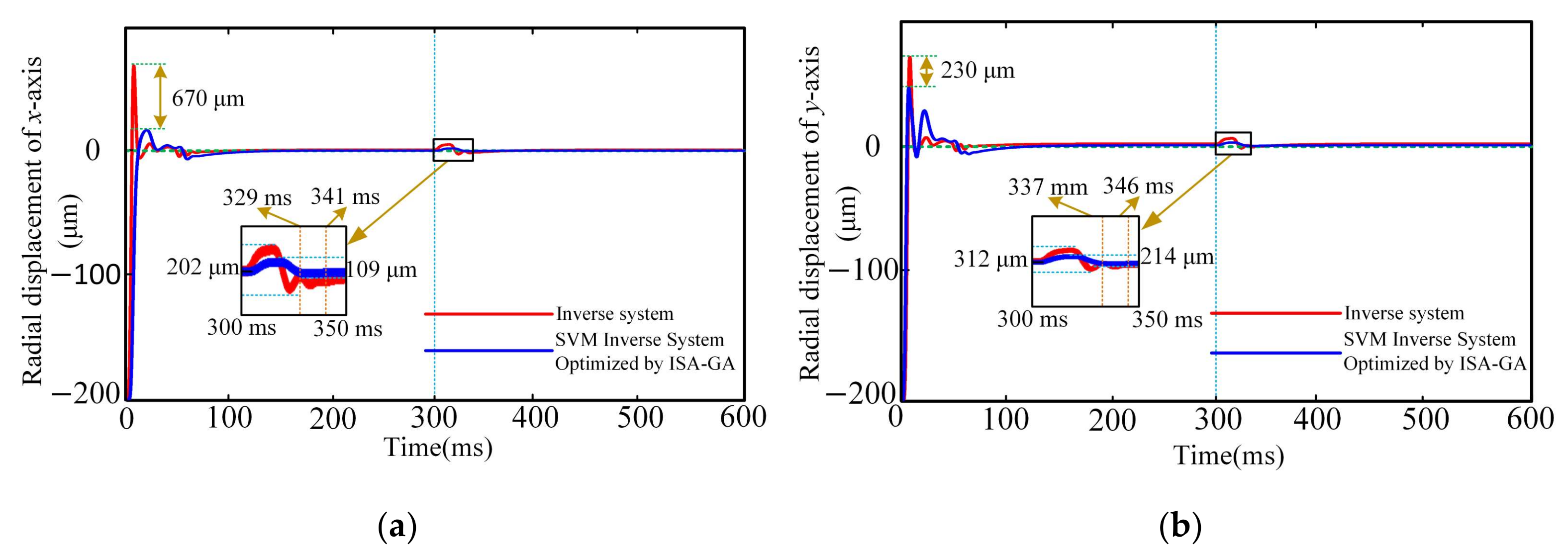
5.1. Analysis of Simulation Results

To verify the effectiveness of the proposed decoupling control strategy, a comparative analysis is conducted on the displacement, speed, and flux linkage response waveforms under both the inverse system decoupling control strategy and the proposed SVM inverse system decoupling control strategy optimized by lSA-GA. The comparison illustrates the superiority of the proposed decoupling control method.
Figure 13 presents the radial displacement responses along the x-axis and y-axis under both inverse system decoupling control strategy and the proposed decoupling control strategy, with the radial displacements of the x-axis and y-axis set to 0 μm, respectively. From Figure 13a, it can be seen that compared with the inverse system decoupling control strategy, the maximum offset of the proposed decoupling control on the x-axis is significantly reduced when the motor is started, and the starting displacement in the x-axis direction is reduced by 670 μm. When t = 300 ms, the set speed suddenly changes from 3000 r/min to 6000 r/min. The proposed decoupling control takes 329 ms to reach the set value state, while the inverse system decoupling control requires 341 ms, reducing the decoupling control time by 3.7%. And under the decoupling control strategy of the inverse system, the x-axis offset value is 202 μm, and the radial x-axis offset of the proposed decoupling control is 109 μm, reducing the deviation by 85.3%. Figure 13b shows the waveform of the y-axis displacement, which changes similarly to the radial displacement of the x-axis. Under the proposed decoupling control, the initial displacement in the y-axis direction is reduced by 230 μm. When t = 300 ms, the set speed suddenly changes from 3000 r/min to 6000 r/min. The proposed decoupling control takes 337 ms to reach the set value state, while the inverse system decoupling control strategy takes 346 ms, reducing the decoupling control time by 2.7%. Under the inverse system decoupling control strategy, the y-axis offset is 312 μm, while under the proposed decoupling control, the y-axis radial offset is 214 μm, reducing the deviation by 45.8%. This indicates that the rotor can maintain stable suspension and have a faster radial displacement response speed under the ISA-GA SVM inverse system decoupling control strategy.
The speed responses for the inverse system decoupling control and the proposed decoupling control are shown in Figure 14. With the given speed signals of 3000 r/min and 6000 r/min, respectively, the speed reaches 3000 r/min in 52 ms under inverse system decoupling control, while it takes only 41 ms to reach the same speed when using the proposed decoupling control, and the time was shortened by 26.8%. At t = 300 ms, when the set speed increases from 3000 r/min to 6000 r/min, the speed reaches 6000 r/min after 97 ms with inverse system decoupling control, whereas it takes only 64 ms with the proposed decoupling control, reducing the time by 51.6%. The proposed decoupling control not only shortens the response time but also enhances the initial performance of CCR-BIM. Figure 15 illustrates the comprehensive evaluation of the performance of both the inverse system decoupling control and the proposed decoupling control. The evaluation involves observing and analyzing the speed response characteristics of the system during normal motor operation and under sudden load conditions. When loads are suddenly applied at t = 150 ms and t = 450 ms, respectively, the speed of CCR-BIM exhibits significant fluctuations under inverse system decoupling control, recovering to the given speed after t = 180 ms and t = 490 ms, respectively. However, under the proposed decoupling control, the speed experiences only slight fluctuations upon sudden load application and recovers to the given speed after t = 160 ms and t = 460 ms. The proposed decoupling control significantly reduces the speed recovery time, demonstrating a faster decoupling control response.
Figure 15 presents the flux linkage responses of two decoupling control strategies with an initial flux linkage of 0.54 Wb. The CCR-BlM is started at t = 0 ms, and during the startup process, the flux linkage response output by the proposed decoupling control is more sensitive. When a load is suddenly applied at t = 300 ms, the flux linkage drops from 0.54 Wb to 0.48 Wb. Under the proposed decoupling control, the flux linkage waveform exhibits smaller fluctuations and recovers more quickly than under the inverse decoupling control. During operation, the flux linkage waveform output by the proposed decoupling method is smoother.
Figure 13, Figure 14 and Figure 15 show that the proposed decoupling control exhibits effective decoupling of x-axis and y-axis radial displacements, velocity responses, and flux linkage, with rapid response times.

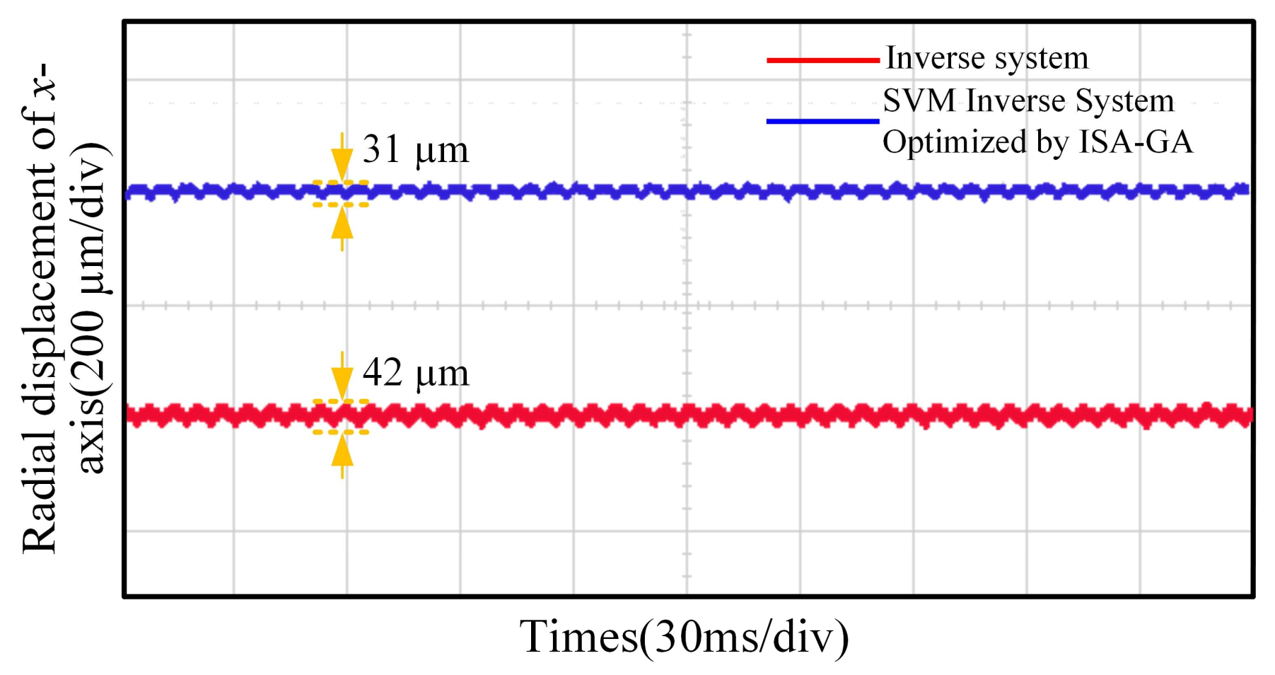
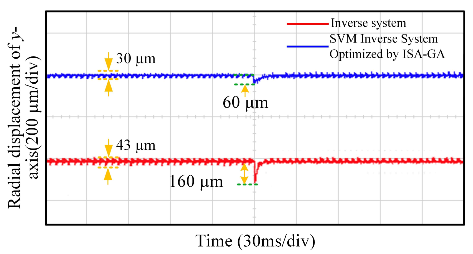
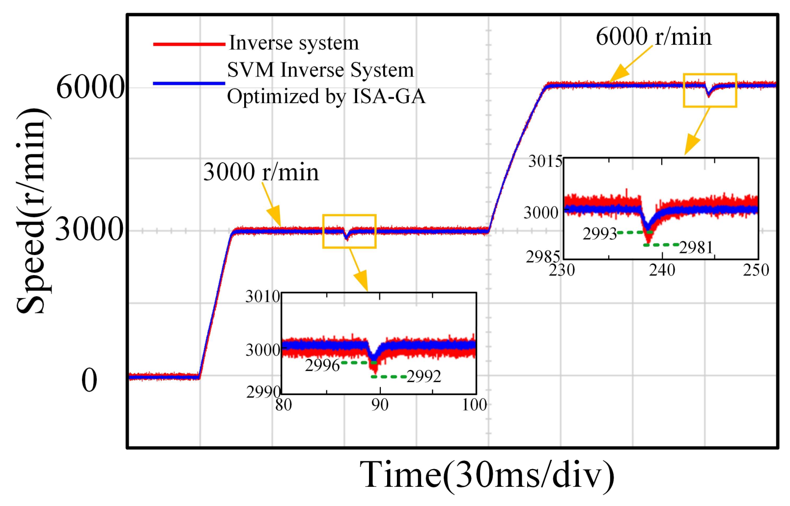
5.2. Analysis of Experimental Results

To further validate the effectiveness of the proposed decoupling control strategy, experimental verification was conducted on a two-degree-of-freedom CCR-BIM. Figure 16 depicts the experimental prototype platform, which primarily consists of CCR-BlM and its peripheral equipment, including control and drive components such as the DSP main control board, power drive circuit board, and interface circuit board. The TMS320F28335 is used with an interrupt frequency of 10 kHz. The torque control algorithm and suspension control algorithm are completed in the same interrupt process. The decoupling control algorithm in this method consumes 10 μs of time; therefore, the real-time performance can meet the control requirements.
To achieve closed-loop feedback control of rotational speed and displacement, the platform integrates monitoring equipment such as optical encoders and eddy current sensors. Additionally, to measure and collect experimental data, the setup includes measurement equipment like a host computer (PC), an oscilloscope, a torque meter, and a dynamometer. The DSP main control board primarily controls the torque and suspension sections. The power drive board drives two sets of windings, while the interface circuit board performs voltage boosting and signal amplification between the DSP main control board and the power drive board. The optical encoder and eddy current sensor are responsible for acquiring and modulating the rotational speed and shaft displacement of CCR-BIM, respectively. The oscilloscope, torque meter, and dynamometer are mainly used to collect or monitor corresponding parameters and transmit them to the PC.
Figure 17 presents the x-axis displacement responses under both the inverse system decoupling control and the proposed SVM inverse control optimized by ISA-GA. In the experimental platform, a position value of 0 μm is given for both cases. Under the inverse decoupling control, the maximum radial deviation of the rotor center in the x-direction is 42 μm. However, under the proposed decoupling control, the maximum radial deviation of the rotor center in the x-direction is only 31 μm, reducing the displacement deviation by 35.5%.
Figure 18 presents the y-axis displacement response under both the inverse system decoupling control and the proposed decoupling control. Under the inverse system decoupling control, the maximum radial deviation of the rotor center in the y-direction is 43 μm. However, under the proposed decoupling control, the maximum radial deviation of the rotor center in the y-direction is only 30 μm, reducing the vibration offset by 43.3%. Additionally, to verify the disturbance rejection performance, a disturbance experiment was conducted in the y-axis direction. Under the same disturbance load conditions, the disturbance deviation with the inverse system decoupling control is 160 μm, and it takes longer to recover to the set value. In contrast, the disturbance deviation with the proposed decoupling control is 60 μm, with a shorter recovery time, reducing the disturbance offset by 62.5%. This indicates that the proposed decoupling control exhibits better decoupling effects and can handle external disturbances more quickly. By comparison, under the proposed decoupling control, the CCR-BlM can achieve displacement decoupling control and exhibit superior disturbance rejection performance.
Figure 19 presents the speed response under both the inverse system decoupling control and the proposed decoupling control. When t = 0 ms, the startup speed reaches its stable value more quickly under the proposed decoupling control. When t = 150 ms, as the speed increases from 3000 r/min to 6000 r/min, the proposed decoupling control achieves a stable speed faster, with smaller speed fluctuations and greater stability. In contrast, under the inverse decoupling control, the speed response waveform exhibits significant jitter. During stable operation at a set speed of 3000 r/min, when a sudden load of 12 N·m is applied to CCR-BlM at t = 90 ms, the speed fluctuation under the proposed decoupling control is 4 r/min, and it recovers to the set speed in a shorter time. Under the inverse system decoupling control, the speed fluctuation is 8 r/min, and the fluctuation has decreased by 50.0%. Similarly, during stable operation at a set speed of 6000 r/min, when a sudden load of 12 N·m is applied to CCR-BIM at t = 240 ms, the speed fluctuation under the proposed decoupling control is 7 r/min, and it recovers to the set speed more quickly. In contrast, under the inverse system decoupling control, the speed fluctuation is 19 r/min, and the fluctuation has decreased by 63.2%. These results demonstrate that the proposed decoupling control is faster and has stronger disturbance rejection capabilities.
In summary, the proposed decoupling control achieves decoupling of radial displacements along the x-axis and y-axis, flux linkage and speed. The control demonstrates rapid decoupling and strong disturbance rejection capabilities. The superiority of the proposed decoupling control is verified.

6. Conclusions

This study presents a novel inverse system decoupling control strategy for the composite cage rotor bearingless induction motor (CCR-BIM) by integrating a support vector machine (SVM) optimized with an improved simulated annealing-genetic algorithm (ISA-GA). The primary objective was to address the inherent nonlinearity and strong coupling among rotor displacement, speed, and flux linkage in CCR-BIM systems. The key contributions are summarized as follows:
(1)
The ISA-GA introduces adaptive crossover and mutation operators, effectively mitigating premature convergence and improving global search efficiency. This enables precise optimization of SVM kernel parameters, resulting in a high-accuracy inverse system model.
(2)
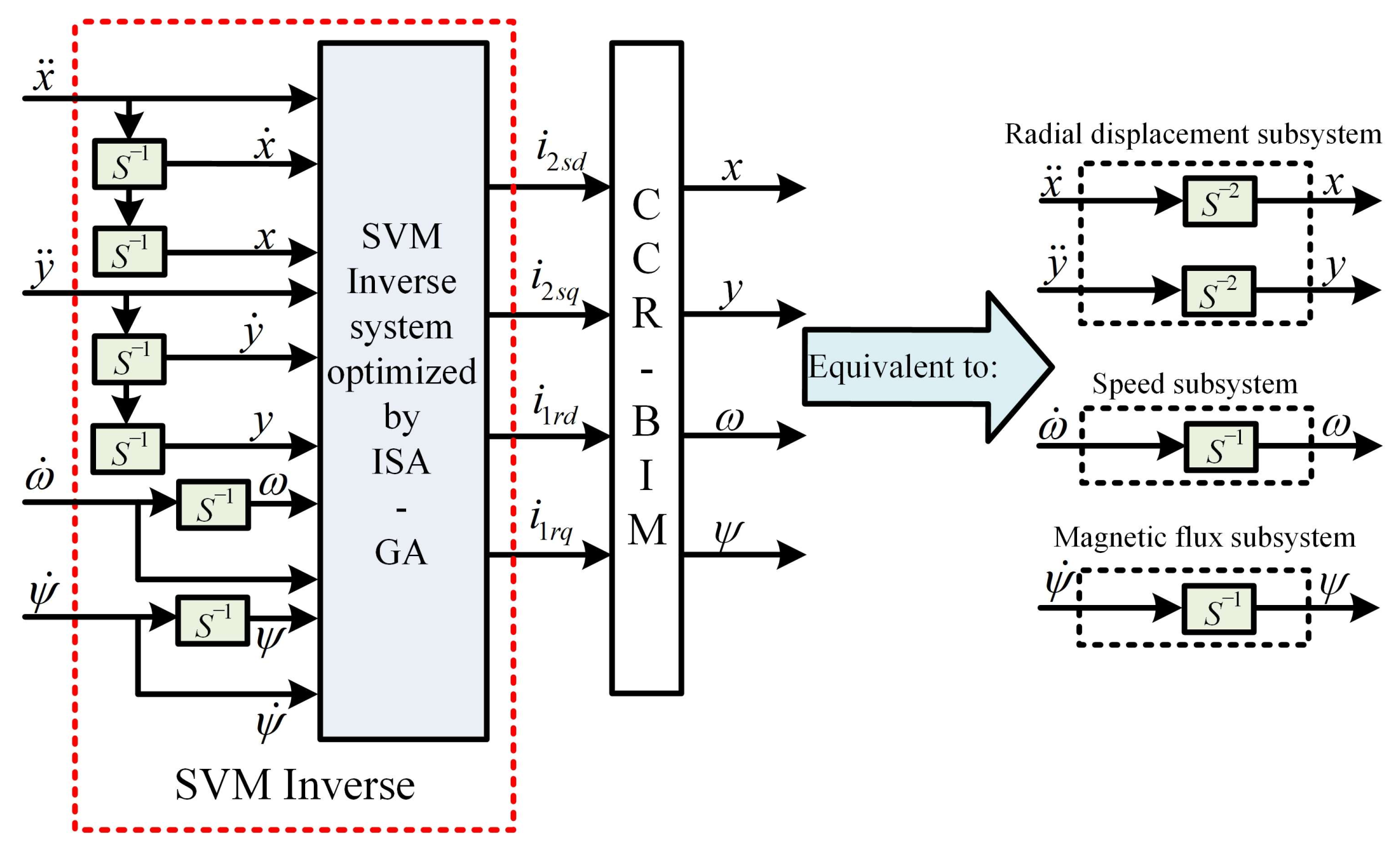
By cascading the optimized SVM inverse model with the original system, the nonlinear CCR-BIM is transformed into a pseudo-linear system, achieving independent control of rotor displacement, speed, and flux linkage.
(3)
Simulation and experimental results demonstrated significant improvements over traditional inverse decoupling control. For instance, radial displacement deviations in the x- and y-axes were reduced by 35.5% and 43.3%, respectively, under dynamic conditions. Additionally, the speed fluctuation decreased by 50.0% and 63.2% at 3000 r/min and 6000 r/min, respectively. These metrics confirm the superior dynamic and static decoupling performance of the proposed strategy.

Author Contributions

C.L.: Data curation, Formal analysis, Methodology, Software, Validation, Writing—original draft; J.C.: Formal analysis, Supervision, Validation, Writing—review and editing; Q.D.: Supervision, Software, Writing—review and editing; G.Z.: Investigation, Funding acquisition, Writing—review and editing; J.F.: Investigation, Project administration, Writing—review and editing; L.Z.: Formal analysis, Software, Visualization; C.D.: Data curation: Formal analysis, Project administration; Y.Z.: Visualization, Writing—review and editing. All authors have read and agreed to the published version of the manuscript.

Funding

This work was supported by the Open Fund of Anhui Undergrowth Crop Intelligent Equipment Engineering Research Center (AUCIEERC-2022-01), Anhui Undergrowth Crop Intelligent Equipment Engineering Research Center (2022AH010091), the Doctoral Research and Innovation Project of Jiangsu Province (KYCX213362), and Start-up Fund for Distinguished Scholars of West Anhui University.

Data Availability Statement

Data available upon a request to the author.

Conflicts of Interest

The author declares no conflicts of interest.

Abbreviations

CCR-BIMComposite Cage Rotor Bearingless Induction Motor
IMInduction Motor
SVMSupport Vector Machine
ISA-GAImproved Simulated Annealing-Genetic Algorithm
MMFMagnetomotive force
(EMEs)Induced Electromotive Forces
KKTKarush–Kuhn–Tucker
SMOSequential Minimal Optimization
PWMPulse Width Modulation

References

  1. Garcia-Calva, T.; Morinigo-Sotelo, D.; Fernandez-Cavero, V.; Romero-Troncoso, R. Early Detection of Faults in Induction Motors—A Review. Energies 2022, 15, 7855. [Google Scholar] [CrossRef]
  2. Yakhni, M.F.; Cauet, S.; Sakout, A.; Assoum, H.; Etien, E.; Rambault, L.; El-Gohary, M. Variable speed induction motors’ fault detection based on transient motor current signatures analysis: A review. Mech. Syst. Signal Process. 2023, 184, 109737. [Google Scholar] [CrossRef]
  3. Shiravani, F.; Alkorta, P.; Cortajarena, J.A.; Barambones, O. An enhanced sliding mode speed control for induction motor drives. Actuators 2022, 11, 18. [Google Scholar] [CrossRef]
  4. Gundewar, S.K.; Kane, P.V. Condition monitoring and fault diagnosis of induction motor. J. Vib. Eng. Technol. 2021, 9, 643–674. [Google Scholar] [CrossRef]
  5. Azab, M. A Review of Recent Trends in High-Efficiency Induction Motor Drives. Vehicles 2025, 7, 15. [Google Scholar] [CrossRef]
  6. Supreeth, D.K.; Bekinal, S.I.; Chandranna, S.R.; Doddamani, M. A review of superconducting magnetic bearings and their application. IEEE Trans. Appl. Supercond. 2022, 32, 3800215. [Google Scholar] [CrossRef]
  7. Lu, C.; Yang, Z.; Sun, X.; Ding, Q. Vibration compensation control strategy of composite cage rotor bearingless induction motor based on fuzzy coefficient adaptive-linear-neuron method. ISA Trans. 2024, 154, 455–464. [Google Scholar] [CrossRef]
  8. Lu, C.; Yang, Z.; Sun, X.; Ding, Q. Design and Multi-Objective Optimization of a Composite Cage Rotor Bearingless Induction Motor. Electronics 2023, 12, 775. [Google Scholar] [CrossRef]
  9. Hearst, M.A.; Dumais, S.T.; Osuna, E.; Platt, J.; Scholkopf, B. Support vector machines. IEEE Intell. Syst. Their Appl. 1998, 13, 18–28. [Google Scholar] [CrossRef]
  10. Cervantes, J.; Garcia-Lamont, F.; Rodríguez-Mazahua, L.; Lopez, A. A comprehensive survey on support vector machine classification: Applications, challenges and trends. Neurocomputing 2020, 408, 189–215. [Google Scholar] [CrossRef]
  11. Tharwat, A. Parameter investigation of support vector machine classifier with kernel functions. Knowl. Inf. Syst. 2019, 61, 1269–1302. [Google Scholar] [CrossRef]
  12. Chen, P.H.; Fan, R.E.; Lin, C.J. A study on SMO-type decomposition methods for support vector machines. IEEE Trans. Neural Netw. 2024, 17, 893–908. [Google Scholar] [CrossRef] [PubMed]
  13. Yang, Z.; Sun, X.; Zhu, H. Decoupling control for bearingless synchronous reluctance motor based on support vector machine inverse. Int. J. Model. Identif. Control. 2015, 23, 24–32. [Google Scholar] [CrossRef]
  14. Yang, K.; Zhu, Z.; Sun, Y. Decoupling control of single winding bearingless switched reluctance motors based on support vector machine inverse system. In Proceedings of the 2014 17th International Conference on Electrical Machines and Systems (ICEMS), Hangzhou, China, 22–25 October 2014; pp. 1829–1833. [Google Scholar]
  15. Xu, B.; Zhu, H.; Wang, X. Decoupling control of outer rotor coreless bearingless permanent magnet synchronous motor based on least squares support vector machine generalized inverse optimized by improved genetic algorithm. IEEE Trans. Ind. Electron. 2021, 69, 12182–12190. [Google Scholar] [CrossRef]
  16. Wang, Z.Q.; Huang, X.L. Nonlinear decoupling control for bearingless induction motor based on support vector machines inversion. Trans. China Electrotech. Soc. 2015, 30, 164–170. [Google Scholar]
  17. Yang, Z.; Wang, D.; Sun, X.; Wu, J. Speed sensorless control of a bearingless induction motor with combined neural network and fractional sliding mode. Mechatronics 2022, 82, 102721. [Google Scholar] [CrossRef]
  18. Pei, T.; Li, D.; Liu, J.; Li, J.; Kong, W. Review of bearingless synchronous motors: Principle and topology. IEEE Trans. Transp. Electrif. 2022, 8, 3489–3502. [Google Scholar] [CrossRef]
  19. Hemenway, N.R.; Gjemdal, H.; Severson, E.L. New three-pole combined radial–axial magnetic bearing for industrial bearingless motor systems. IEEE Trans. Ind. Appl. 2021, 57, 6754–6764. [Google Scholar] [CrossRef]
  20. Sun, C.; Yang, Z.; Sun, X.; Ding, Q. An Improved Mathematical Model for Speed Sensorless Control of Fixed Pole Bearingless Induction Motor. IEEE Trans. Ind. Electron. 2023, 71, 1286–1295. [Google Scholar] [CrossRef]
  21. Ding, Q.; Yang, Z.; Sun, X.; Lu, C. Correction of the suspension force expression and the control compensation study in a bearingless induction motor. Electr. Eng. 2022, 104, 2457–2469. [Google Scholar] [CrossRef]
  22. Roy, A.; Chakraborty, S. Support vector machine in structural reliability analysis: A review. Reliab. Eng. Syst. Saf. 2023, 233, 109126. [Google Scholar] [CrossRef]
  23. Wang, B.; Zhang, X.; Xing, S.; Sun, C.; Chen, X. Sparse representation theory for support vector machine kernel function selection and its application in high-speed bearing fault diagnosis. ISA Trans. 2021, 118, 207–218. [Google Scholar] [CrossRef] [PubMed]
  24. Nguyen, H.; Bui, X.N.; Choi, Y.; Lee, C.W.; Armaghani, D.J. A novel combination of whale optimization algorithm and support vector machine with different kernel functions for prediction of blasting-induced fly-rock in quarry mines. Nat. Resour. Res. 2021, 30, 191–207. [Google Scholar] [CrossRef]
  25. He, F.; Ye, Q. A bearing fault diagnosis method based on wavelet packet transform and convolutional neural network optimized by simulated annealing algorithm. Sensors 2022, 22, 1410. [Google Scholar] [CrossRef]
  26. Okwu, M.O.; Tartibu, L.K. Metaheuristic Optimization: Nature-Inspired Algorithms Swarm and Computational Intelligence, Theory and Applications; Springer: Berlin/Heidelberg, Germany, 2021; pp. 125–132. [Google Scholar]
Figure 1. Principle of the suspension force.
Actuators 14 00125 g001
Figure 2. Topology structure of the CCR-BIM.
Actuators 14 00125 g002
Figure 3. Stator structure and stator winding distribution. (a) Stator structure. (b) Distribution of stator winding.
Actuators 14 00125 g003
Figure 4. Structure of composite cage rotor.
Actuators 14 00125 g004
Figure 5. Structure of inner rotor.
Actuators 14 00125 g005
Figure 6. Special cage structure. (a) Bar assembly structure. (b) Cage structure.
Actuators 14 00125 g006
Figure 7. Current distribution of cage structure. (a) P1 = 1. (b) P2 = 2.
Actuators 14 00125 g007
Figure 8. Sample point processing. (a) Sample points are inseparable. (b) Inseparable within the sample space. (c) Sample points are separable.
Actuators 14 00125 g008
Figure 9. ISA-GA flowchart.
Actuators 14 00125 g009
Figure 10. Topology diagram of SVM optimized by ISA-GA.
Actuators 14 00125 g010
Figure 11. SVM inverse system structure.
Actuators 14 00125 g011
Figure 12. Decoupling control block diagram.
Actuators 14 00125 g012
Figure 13. Radial displacement response of x-axis and y-axis. (a) x-axis. (b) y-axis.
Actuators 14 00125 g013
Figure 14. Speed response waveform.
Actuators 14 00125 g014
Figure 15. Response waveform of magnetic flux.
Actuators 14 00125 g015
Figure 16. Experimental platform for CCR-BIM.
Actuators 14 00125 g016
Figure 17. Response waveform of x-axis displacement.
Actuators 14 00125 g017
Figure 18. Response waveform of y-axis displacement.
Actuators 14 00125 g018
Figure 19. Response waveform of speed.
Actuators 14 00125 g019
Table 1. CCR-BIM parameters.
ParameterValueParameterValue
Rated power (P1/P2)1.5/0.5 kWRated speed3000 r/min
Number of poles (P1/P2)1/2Wire diameter of windings2.5 mm
Number of turns (N1/N2)60/30Rotor outer diameter64.2 mm
Number of stator slots24 Thickness of outer rotor1.8 mm
Number of rotor slots20 Outer diameter of inner rotor60.6 mm
Voltage of torque winding310 VInner diameter of rotor20.5 mm
Current of suspension winding0.5 AInner diameter of stator64.6 mm
Rotor weight2.8 kgRotor length80 mm
Stator and rotor silicon steelDW540_50Air gap length0.4 mm
Moment of inertia7.7 g·m2Outer diameter of stator122 mm
Disclaimer/Publisher’s Note: The statements, opinions and data contained in all publications are solely those of the individual author(s) and contributor(s) and not of MDPI and/or the editor(s). MDPI and/or the editor(s) disclaim responsibility for any injury to people or property resulting from any ideas, methods, instructions or products referred to in the content.

