Coupled Dynamics Modeling and Validation of Maglev Vehicle and Bridge Systems

Abstract

To address the vehicle-bridge coupling vibration issue of the Qingyuan Maglev Tourist Line, it is necessary to establish a maglev vehicle–bridge coupling dynamics simulation model that reflects the actual line conditions. Based on the vehicle and bridge structural parameters of the Qingyuan Maglev Tourist Line, this paper utilizes multi-body dynamics simulation software to create a medium–low-speed maglev vehicle dynamics model, and employs finite element software to construct a bridge model. Using the modal reduction method, the bridge finite element model is imported into the vehicle dynamics model through a rigid–flex coupling interface, establishing a medium–low-speed maglev vehicle suspension system–bridge coupling dynamics model. The accuracy of the established coupling simulation model was verified by comparing the simulation data from the coupling model with the dynamic response measured data from the Qingyuan Maglev Tourist Line. Finally, the impact of different control parameters on the vehicle–bridge coupling system was calculated, and the results indicate that selecting appropriate suspension control parameters can reduce the coupling vibration response between the maglev vehicle and the bridge. The main work of this paper is closely related to engineering, modeling based on the actual maglev line’s vehicle and bridge parameters, and validating the model through the dynamic test results of the line, laying the foundation for the suppression of maglev vehicle–bridge coupling vibration and system optimization.

1. Introduction

In recent years, medium- and low-speed maglev transportation has garnered increasing attention in urban transit due to its advantages such as low noise, low vibration, and pollution-free operation. Scholars both domestically and internationally have conducted research on the dynamic characteristics of maglev train–bridge coupling systems, proposing a series of vibration suppression and vehicle stability optimization methods based on vehicle and track structure parameters as well as suspension control parameters. The Qingyuan Maglev Tourist Line commenced trial operations in February 2024. This paper takes the Qingyuan Maglev Tourist Line as the research subject, conducting dynamic modeling of the coupling system and model validation based on measured data, laying the groundwork for the analysis of medium- and low-speed maglev vehicle–bridge coupling vibration characteristics, vibration suppression, and stability optimization research.

The vibration of the vehicle is directly related to driver safety and passenger comfort. H Nahvi et al. [1] collected vibration signals of vehicles driving on different road surfaces and at various speed conditions, evaluating the characteristics of vibration transmission to passengers by calculating parameters such as power spectral density. Ahn S J et al. [2] experimentally studied the discomfort of seated test subjects under different vertical mechanical shocks, finding that the discomfort growth rate gradually decreases in the range of 0.5 Hz to 4 Hz, and the human body is most sensitive to vibrations in the range of 4 Hz to 12.5 Hz. Zhang Bingqiang [3] established a vehicle–road surface system coupling vibration model, conducting in-depth research on vehicle ride comfort. The results showed that vehicle load rate has a certain impact on ride comfort, suspension stiffness has a significant impact on ride comfort, larger suspension stiffness is detrimental to vehicle ride comfort, and road surface irregularity grade has a considerable impact on ride comfort. Hou Lei et al. [4] studied the ride comfort of full-size high-speed maglev trains under different speed conditions. The research results indicated that the comfort of the passengers on such trains deteriorates with as the speed increases, the ride comfort value at the front of the train is the highest compared to other positions, the rear is the second most comfortable area of the train, and the middle has the best ride comfort overall. At speeds below 380 km/h, lateral comfort is worse than vertical comfort, while at speeds above 380 km/h, vertical comfort is worse than lateral comfort, and longitudinal comfort is always the best.

In terms of the principle of vehicle–track coupling vibration and vibration suppression research, foreign scholars started to study this earlier. Zhang L et al. [5] proposed a method for establishing and validating a vehicle–track coupling dynamics model through in situ vibration tests and model updating, and used it to study the impact of track random irregularities on the distribution of electromagnetic forces in high-speed maglev systems. Wang et al. [6,7,8] used Abaqus software to establish a high-speed maglev vehicle and track model considering elastic supports, achieving coupling dynamics analysis between the vehicle and track through self-programmed procedures, and systematically studied the impact of track geometric parameters such as transition curves on vehicle–bridge coupling vibration. Also focusing on vehicle–bridge coupling, Dmitry Pogorelov, Wang K et al. [9,10] studied vehicle–bridge coupling vibration by coupling bridge models in ANSYS with train models in SIMPACK or UM. However, due to the use of modal superposition or modal synthesis methods, this method has certain limitations with regard to calculating high-frequency local modes and complex bridge vibration responses. Huang J Y [11] proposed three numerical models, conducting in-depth research on the vibration characteristics of maglev trains under different speeds and suspension system parameters. By analyzing resonance and cancellation conditions, they derived dynamic amplification criteria for evaluating guideway responses and emphasized the significant impact of suspension system parameters on ride comfort. Kim K J et al. [12] established a detailed model considering spatial degrees of freedom for maglev vehicles, active control, track irregularities, and flexible tracks, simulating and analyzing the dynamic response of bridges and vehicle suspension stability when maglev trains are statically suspended or passing at low speeds, pointing out that the structural characteristics of track beams and stable control algorithms are crucial for suppressing vehicle–bridge coupling resonance.

Domestic scholars have also achieved many results in research on maglev vehicle–bridge coupling vibration. Zeng Jiewei [13] conducted maglev vehicle–track coupling vibration simulation from the perspective of suspension control characteristics, analyzing the impact of main controller parameters on the vibration of the coupling system, and based on vibration tests of the Changsha Maglev Express Line, demonstrated through simulation and testing that appropriate controller parameters can maintain stable suspension of the vehicle. Zhou Danfeng [14] proposed an adaptive vibration control method with an identifier, which was capable of real-time identification of track modal parameters and input–output gain coefficients, thereby generating corresponding control laws to suppress track self-excited vibration. Wang et al. [15] analyzed the mechanism of vertical resonance of bridges caused by maglev trains, showing that low-degree resonance in bridges is caused by the cyclic loading frequency of adjacent electromagnetic forces, and normal-speed resonance is caused by the inherent frequency of electromagnetic suspension forces. Li Yiyang [16] established a coupling dynamics model of maglev trains and steel box girders with different beam heights, simulating the vibration situation when trains pass bridges at high speeds, and analyzed the reasons for larger vibrations at low speeds. Li Xiaozhen et al. [17,18,19,20,21] found that F-rails have a significant impact on the coupling vibration of medium- and low-speed maglev trains and bridge systems. By establishing detailed numerical models, they conducted in-depth analysis of the impact of F-rails on system dynamic responses and explored the impact of different parameters on the vibration of low-lying beams. Yang Jizhong et al. [22] used Midas and UM software to establish a maglev train–bridge coupling dynamics model that included a maglev control system, simulating the vibration situation when maglev trains pass simply supported box girders at different speeds, and conducted in-depth analysis of the dynamic responses of trains and bridges.

The main aim of this paper is to establish a maglev vehicle–bridge coupling dynamics model that reflects actual line conditions. Taking the Qingyuan Maglev Tourist Line as the research subject, this paper established a dynamics model considering the coupling of vehicles, bridges, and suspension systems, and validated the accuracy of the model through on-site maglev vehicle and bridge dynamic response test data from Qingyuan. Finally, the impact of suspension control parameters on the coupling system was analyzed, providing references for optimizing system design and improving train operating performance.

2. Vehicle Dynamics Model

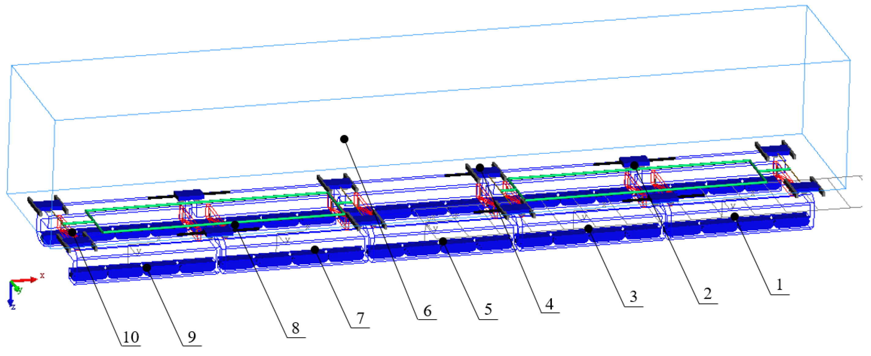
As shown in Figure 1, the suspension frame structure of the Qingyuan maglev vehicle consists of a lateral sliding mechanism, a guidance mechanism, air springs, a traction rod mechanism, suspension modules, anti-roll beams, and electromagnets. Two sets of anti-roll beams connect the left and right suspension modules. The suspension module structure is mainly composed of an upper longitudinal beam, an electromagnet mounting arm, and traction and braking components. The upper longitudinal beam primarily includes a linear traction motor, an air spring base, and support wheels, among other structures. Each set of anti-roll beams is made up of two plate beams, which are connected by two hangers. Each suspension electromagnet module contains four excitation coils and iron cores, as well as inner and outer pole plates. The electromagnetic force generated by the electromagnets allows the vehicle to levitate above the track.

When modeling the dynamics of the maglev vehicle, based on the multi-body dynamics theory, the vehicle structure is appropriately simplified. All vehicle components are treated as rigid bodies, and the suspension system is simulated as spring-damping elements, taking into account the main structures and their relative motion relationships.

A single car body is equipped with five suspension frame modules, which are connected to the car body through air springs at the four corners of the suspension frame. A lateral sliding platform is also installed between the car body and the suspension frame, divided into movable and fixed sliding platforms. Among them, the second and fifth positions are fixed sliding platforms, where the suspension frame is connected to the sliding platform through lateral tie rods, and the car body is fixedly connected to the sliding platform. The first, third, fourth, and sixth positions are movable sliding platforms, where the car body is connected to the movable sliding platform through linear bearings. Additionally, two sets of forced guidance mechanisms are installed, connecting the first and second and the fourth and fifth suspension frames, respectively, to improve the vehicle’s curve negotiation capability. The motion relationships of the main vehicle structures are shown in

Table 1. Degrees of freedom for rigid body motion of maglev vehicles.

Components	Degrees of Freedom
	Longitudinal	Lateral	Vertical	Roll	Pitch	Yaw
Vehicle Body	✓	✓	✓	✓	✓	✓
Left Suspension Module	✓	✓	✓	✓	✓	✓
Right Suspension Module	✓	✓	✓	✓	✓	✓
Middle Slide		✓
Leaf Beam						✓
Suspension Rod				✓
Transverse Tie Rod				✓		✓

. The single-car maglev vehicle dynamics model established in this paper is shown in Figure 2, with a total of 97 degrees of freedom.

3. Bridge Model

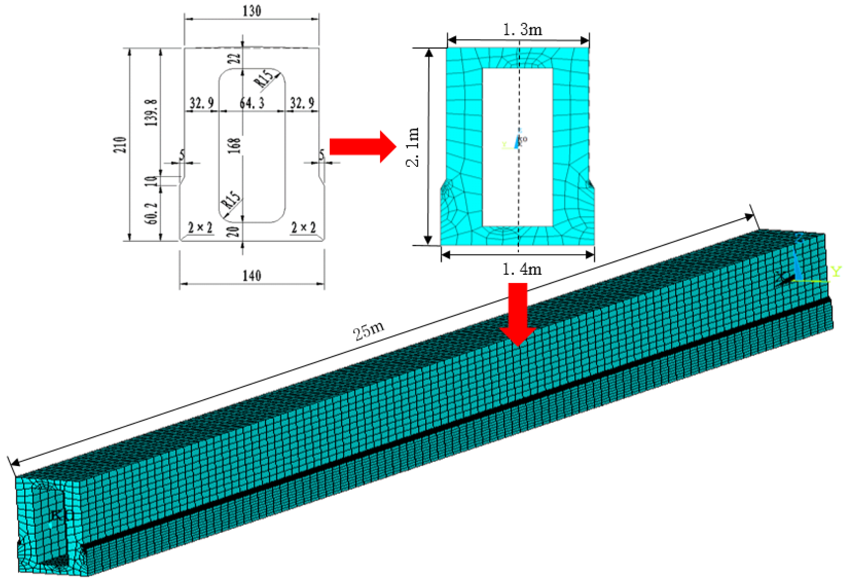
The track girder cross-section type of the Qingyuan Line is a single-box, single-cell, constant-height simply supported girder. The top width of the box girder is 1.3 m, the bottom width is 1.4 m, and the girder height is 2.1 m. The concrete density is 26.5 kN/m³, and the total secondary dead load for a single track is 12 kN/m. The box girder is constructed using C50 concrete, with compressive strength of $f_c=33.5$ MPa, tensile strength of $f_{ct}=3.1$ MPa, and an elastic modulus of $Ec=3.55\times {10}^4$ MPa. The outline of the cross-section of the simply supported girder in the straight section is shown in Figure 3. On the Qingyuan Line, the straight sections consist of simply supported girders with three span lengths: 20 m, 22 m, and 25 m. For this study, a bridge span of 25 m is selected for calculation.

The Beam188 element is used for finite element modeling of the bridge, and spring elements are employed to simulate the support constraints at the ends of the simply supported girder. A constrained modal analysis is performed on the bridge finite element model, and the frequencies of the first 10 modes are summarized in

Table 2. Statistics of the first 10 constrained modal frequencies and mode shapes of the bridge.

Mode Number	Frequency/Hz	Description of Mode Shape
1	5.16	1st Mode—Lateral Bending
2	7.47	1st Mode—Vertical Bending
3	19.57	2nd Mode—Lateral Bending
4	28.44	2nd Mode—Vertical Bending
5	38.27	Longitudinal Stretching
6	40.73	3rd Mode—Lateral Bending
7	41.85	Torsion
8	59.64	3rd Mode Vertical Bending
9	66.11	4th Mode Vertical Bending
10	84.01	Torsion

.

In dynamic simulation calculations, the vibration of the bridge is solved based on the Bernoulli–Euler beam theory using the modal superposition method. By transforming the bridge’s dynamic equations from physical coordinates to modal coordinates, decoupled single-degree-of-freedom system equations are formed and solved. Finally, the calculation results are linearly superimposed and transformed back to physical coordinates to obtain the final vibration response of the bridge. In this paper, the first 10 modes of the bridge are selected for superposition.

The modal superposition method simplifies calculations by reducing the degrees of freedom through the use of the structure’s primary modes. Typically, only low-frequency modes are retained, while high-frequency modes participate less or are truncated during computation, and the influence of high-frequency components is ignored. Complex vibrations in bridges often contain significant high-frequency components, and vehicle–bridge coupling vibrations may involve nonlinear factors, especially during high-frequency vibrations where the nonlinear behavior of the structure may become more pronounced. In such cases, the linear assumptions of the modal superposition method can lead to significant errors in the calculated results.

4. Electromagnetic Force and Control System Model

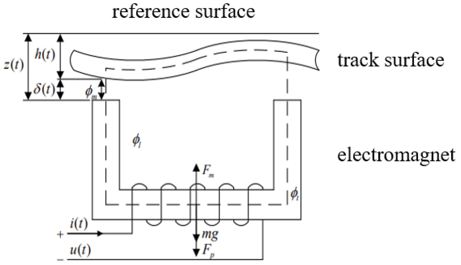
Compared to high-speed maglev trains, medium- and low-speed maglev trains do not have separate guidance electromagnets. Instead, they utilize the lateral component of the levitation force from the levitation electromagnets for guidance, typically with active control only applied to the vertical direction of the electromagnets.

Before deriving the electromagnetic force, the following assumptions are made:

(i)

The lateral displacement of the electromagnets is small.

(ii)

Magnetic leakage is neglected.

(iii)

The magnetic reluctance in the iron core and the guide-way is neglected.

(iv)

The magnetic field intensity in the air gap is uniformly distributed.

In the maglev train, there are a total of 20 levitation control points, each operating independently. The index for these points is set from 1 to 20. The vertical and lateral expressions for the electromagnetic force can be derived as follows:

$$\begin{array}{c}{F}_{y_n}=F_{m_n}{\displaystyle \frac{2{\delta }_n}{\pi W_m}}arctan\left({\displaystyle \frac{\Delta y_n}{{\delta }_n}}\right)(n=1,2,3\dots 20)\end{array}$$

(1)

$$\begin{array}{c}{F}_{z_n}=F_{m_n}\left(1+{\displaystyle \frac{2{\delta }_n}{\pi W_m}}-{\displaystyle \frac{2\Delta y_n}{\pi W_m}}arctan\left({\displaystyle \frac{\Delta y_n}{{\delta }_n}}\right)\right)(n=1,2,3\dots 20)\end{array}$$

(2)

$$\begin{array}{c}{F}_{m_n}={\displaystyle \frac{u_0{N}^{2}A}{4}}{\left({\displaystyle \frac{i_n}{{\delta }_n}}\right)}^2(n=1,2,3\dots 20)\end{array}$$

(3)

The meanings of the symbols in the equation are as follows:

(i)

A represents the effective area of the magnetic pole.

(ii)

N represents the number of turns of the electromagnet coil.

(iii)

i represents the coil current.

(iv)

$\delta$ represents the levitation gap.

(v)

$\Delta y$ represents the displacement of the electromagnet relative to the track.

(vi)

$u_0$ represents the permeability of the air gap.

From the equation, it can be observed that the greater the displacement of the electromagnet, the larger the lateral electromagnetic force and the smaller the vertical electromagnetic force, resulting in a reduced levitation gap. At this point, the controller will increase the current to further adjust the electromagnetic force and levitation gap, continuously making dynamic adjustments.

Unlike traditional wheel-rail trains, maglev trains maintain a certain levitation gap between the vehicle body and the track during operation. The core control objective of the maglev train’s levitation system is to maintain this levitation gap, allowing it to fluctuate around the equilibrium position to ensure the safety and operational comfort of the train, effectively avoiding the risk of collision between the vehicle body and the track. The adjustment of the levitation gap is primarily achieved by controlling the levitation force (i.e., the electromagnetic attraction between the vehicle body and the track). Specifically, the levitation system adjusts the levitation current to change the magnitude of the levitation force, thereby achieving precise control of the levitation gap. Eddy current gap sensors and acceleration sensors are installed on the levitation electromagnets of the maglev train to measure the levitation gap and the acceleration of the electromagnets.

In practical engineering applications, due to significant differences in vehicle structures, track characteristics, and on-site environmental conditions across different maglev lines, the control parameters of the levitation system need to be repeatedly debugged and optimized based on expert experience and the actual operating conditions of the train. This process not only relies on the guidance of theoretical models but also requires dynamic adjustments based on extensive experimental data and operational feedback to ensure the stability and reliability of the system under various working conditions.

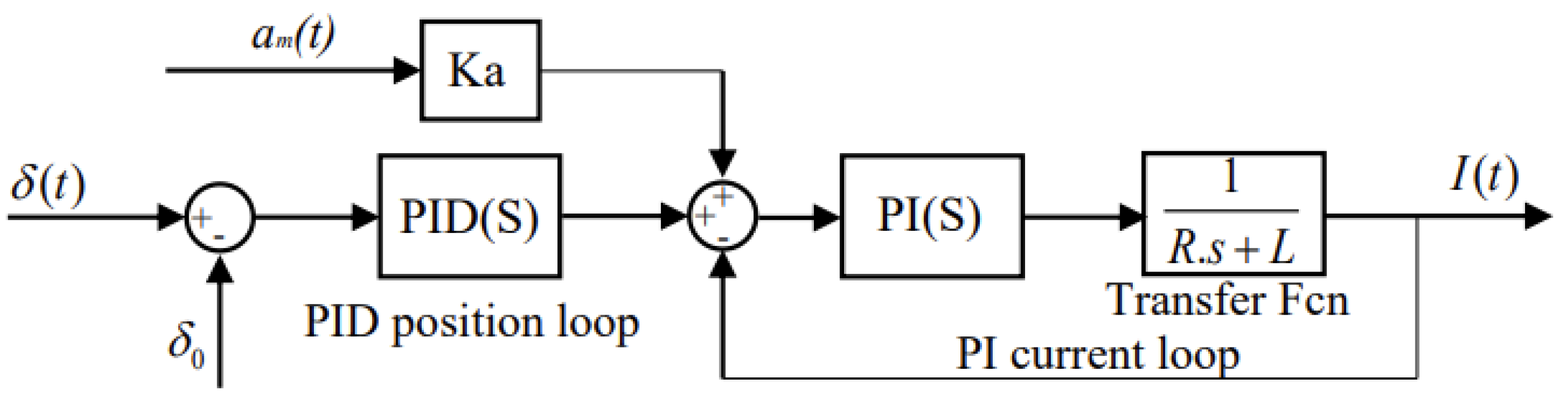
The levitation control system of maglev vehicles adopts a decentralized and independent control approach. The electromagnets of the train are divided into two independent modules, front and rear, each of which is controlled separately. Therefore, when designing the levitation control algorithm, research is conducted on a single module of the electromagnet (referred to as a single-electromagnet system), as shown in Figure 4. Based on Newton’s laws, the vertical dynamic equation of a single electromagnet system can be derived as follows:

$$\begin{array}{c}m\ddot{z}\left(t\right)=mg-F_m(i,\delta )+F_p\left(t\right)\end{array}$$

(4)

In the formula, $F_p\left(t\right)$ represents the external load on the system, and the vertical positional relationships between the reference surface, guide rail, and magnetic pole face are as follows:

$$\begin{array}{c}z\left(t\right)=h\left(t\right)+\delta \left(t\right)\end{array},$$

(5)

According to the principles of electrical circuits, the relationship between the voltage and current in an electromagnet coil is given by the following equation:

$$\begin{array}{c}{u}_n=R_0{i}_n+{\displaystyle \frac{u_0{N}^{2}A}{2{\delta }_n}}{i}_n-{\displaystyle \frac{u_0{N}^{2}A{i}_n}{2{\delta }_n^2}}{\dot{\delta }}_n(n=1,2,3\dots 20)\end{array}$$

(6)

In the equation, $R_0$ represents the resistance of the coil.

Suspension control systems often employ a voltage control strategy. Due to the significant inductance of the electromagnet coil, the inherent delay caused by the inductance can impede the system’s ability to achieve rapid tracking. To address this, a two-level cascade suspension control algorithm, typically consisting of a position loop and a current loop, is generally utilized. The primary position loop facilitates swift adjustment of the suspension gap, while the subsequent current loop ensures that the current can promptly follow the control voltage, thereby mitigating the delay effects induced by the electromagnet’s inductance, the control system is shown in Figure 5.

Primary suspension control typically employs PID control for the suspension gap and acceleration feedback control for the electromagnet. The control law for the electromagnet coil current is as follows:

$$\begin{array}{c}{i}_n\left(t\right)=i_0+k_p\Delta {\delta }_n\left(t\right)+k_d\Delta {\dot{\delta }}_n\left(t\right)+k_i\int \Delta \delta {\left(t\right)}_n+k_a{a}_m(n=1,2,3\dots 20)\end{array}$$

(7)

In the equation, $k_p$, $k_d$, and $k_i$ are the feedback coefficients for the gap, gap velocity, and gap integral, respectively, and $k_a$ represents the feedback coefficient for the electromagnet acceleration.

5. Track Irregularity

The random irregularity of the track is the primary external excitation source affecting the coupled vibration of the maglev vehicle–bridge system. Currently, there is no well-established power spectrum for medium- and low-speed maglev track irregularities that can be directly applied to dynamic calculations. Research by Zhang Geng et al. [23], based on measured data from the Tangshan test line, indicates that the alignment irregularity of medium- and low-speed maglev tracks is close to the German high-disturbance spectrum, while the vertical irregularity is worse than the American Class 6 spectrum. This paper derives spatial samples of irregularities based on the German high-disturbance spectrum and incorporates them into the model for calculation. The roughness coefficient level cutoff frequency of the German track spectrum is shown in

Table 3. Roughness coefficient and cutoff frequency of the German track spectrum.

Track Level	${\mathbf{\Omega }}_{\mathit{c}}$	${\mathbf{\Omega }}_{\mathit{r}}$	${\mathit{A}}_{\mathit{a}}$	${\mathit{A}}_{\mathit{v}}$
Low Interference	0.8246	0.0206	$2.119\times {10}^{-7}$	$4.032\times {10}^{-7}$
High Interference	0.8246	0.0206	$6.125\times {10}^{-7}$	$1.08\times {10}^{-6}$

.

The formula for calculating the power spectral density of German vertical irregularities is as follows:

$$\begin{array}{c}{S}_v(\Omega )={\displaystyle \frac{A_v{\Omega }_c^2}{\left({\Omega }^2+{\Omega }_r^2\right)\left({\Omega }^2+{\Omega }_c^2\right)}}\end{array}$$

(8)

The formula for calculating the power spectral density of alignment irregularities is as follows:

$$\begin{array}{c}{S}_a(\Omega )={\displaystyle \frac{A_a{\Omega }_c^2}{\left({\Omega }^2+{\Omega }_r^2\right)\left({\Omega }^2+{\Omega }_c^2\right)}}\end{array}$$

(9)

6. Maglev Vehicle–Bridge Coupled Dynamics Model

This paper establishes a model based on the structural parameters of the maglev vehicle and track beam from the Qingyuan Maglev Tourist Line. A vehicle dynamics model is developed in Simpack, while a bridge model is created using finite element software. Through the Guyan modal reduction method, the bridge model is imported into Simpack. The dynamic equation for an n-degree-of-freedom system is expressed as follows:

$$\begin{array}{c}M\ddot{u}+Ku=F\left(t\right)\end{array}$$

(10)

In the equation, M represents the mass matrix, K represents the stiffness matrix, u is the displacement vector, and F is the external force. When the degrees of freedom are divided into primary degrees of freedom ($u_m$) and secondary degrees of freedom ($u_s$), the equation is expressed as follows:

$$\begin{array}{c}\left[\begin{array}{cc}{M}_{mws}\hfill & M_{mx}\hfill \\ M_{sw}\hfill & M_{ss}\hfill \end{array}\right]\left[\begin{array}{c}{\ddot{u}}_m\hfill \\ {\ddot{u}}_x\hfill \end{array}\right]+\left[\begin{array}{cc}{K}_{mm}\hfill & K_{mx}\hfill \\ K_{sm}\hfill & K_{sx}\hfill \end{array}\right]\left[\begin{array}{c}{u}_m\hfill \\ u_x\hfill \end{array}\right]=\left[\begin{array}{c}{F}_m\\ F_x\end{array}\right]\end{array}$$

(11)

In the equation, m represents the number of primary degrees of freedom and s represents the number of secondary degrees of freedom. The concept of Guyan reduction is to set $F_s$ = 0 (i.e., neglect the inertial forces of the secondary coordinates). Then, by partitioning the above equation, the coordinate transformation is obtained as follows:

$$\begin{array}{c}{u}_x=-K_{sx}^{-1}{K}_{sm}{u}_m\end{array}$$

(12)

Thus, the displacement relationship is obtained as follows:

$$\begin{array}{c}u=\left[\begin{array}{c}{u}_m\hfill \\ u_s\hfill \end{array}\right]=T{u}_m\end{array}$$

(13)

Where the transformation matrix is

$$\begin{array}{c}T=\left[\begin{array}{c}I\\ -K_{s\mathrm{s}}^{-1}{K}_{sm}\end{array}\right]\end{array}$$

(14)

Substituting the displacement relationship into the original equation, the stiffness matrix and mass matrix after modal reduction are obtained.

$$\begin{array}{c}\begin{array}{c}\hfill K_{red}=T^{\tau }KT\end{array}\end{array}$$

(15)

$$\begin{array}{c}{M}_{red}=T^{\tau }MT\end{array}$$

(16)

At this point, the dynamic equation is simplified to

$$\begin{array}{c}{M}_{red}{\ddot{u}}_m+K_{red}{u}_m=T^{\tau }F\left(t\right)\end{array}$$

(17)

Thus, the free vibration equation after modal reduction is obtained as follows:

$$\begin{array}{c}{M}_{red}{\ddot{u}}_m+K_{rdi}{u}_m=0\end{array}$$

(18)

Assuming a harmonic solution $u_m=\varphi e^{j\omega x}$, substituting it into the equation yields the characteristic equation

$$\begin{array}{c}\left(K_{rd}-{\omega }^2{M}_{rd}\right)\varphi =0\end{array}$$

(19)

Solving this equation yields the natural frequencies $w_i$ and ${\varphi }_i$ modes of the reduced modal system. Using the reduced modes for dynamic calculations, the system’s displacement can be expressed as a linear combination of the modes. By applying Equations (19) and (20), the dynamic response of the system can be determined.

$$\begin{array}{c}{u}_m={\displaystyle \sum _{i=1}^n}{\varphi }_i{q}_i\left(t\right)\end{array}$$

(20)

$$\begin{array}{c}{\ddot{q}}_i+{\omega }^2{q}_i={\varphi }_i^{\tau }{F}_{rdi}\left(t\right)\end{array}$$

(21)

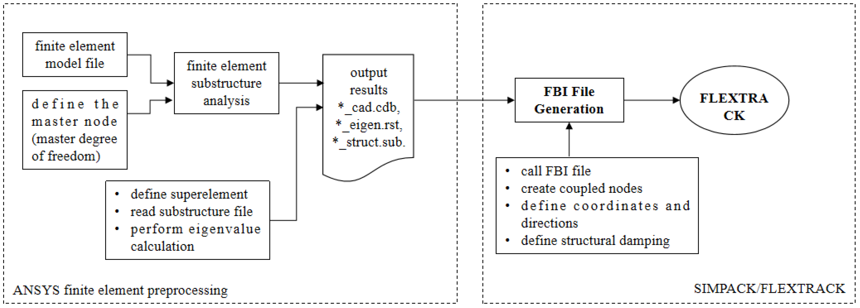
The sub and cdb files generated after modal reduction are processed through SIMPACK’s flexible body coupling interface to generate an FBI file that can be recognized and utilized. Finally, the flexible bridge is imported into SIMPACK using the Flextrack module, and the vehicle is linked to the track through force elements, as shown in Figure 6.

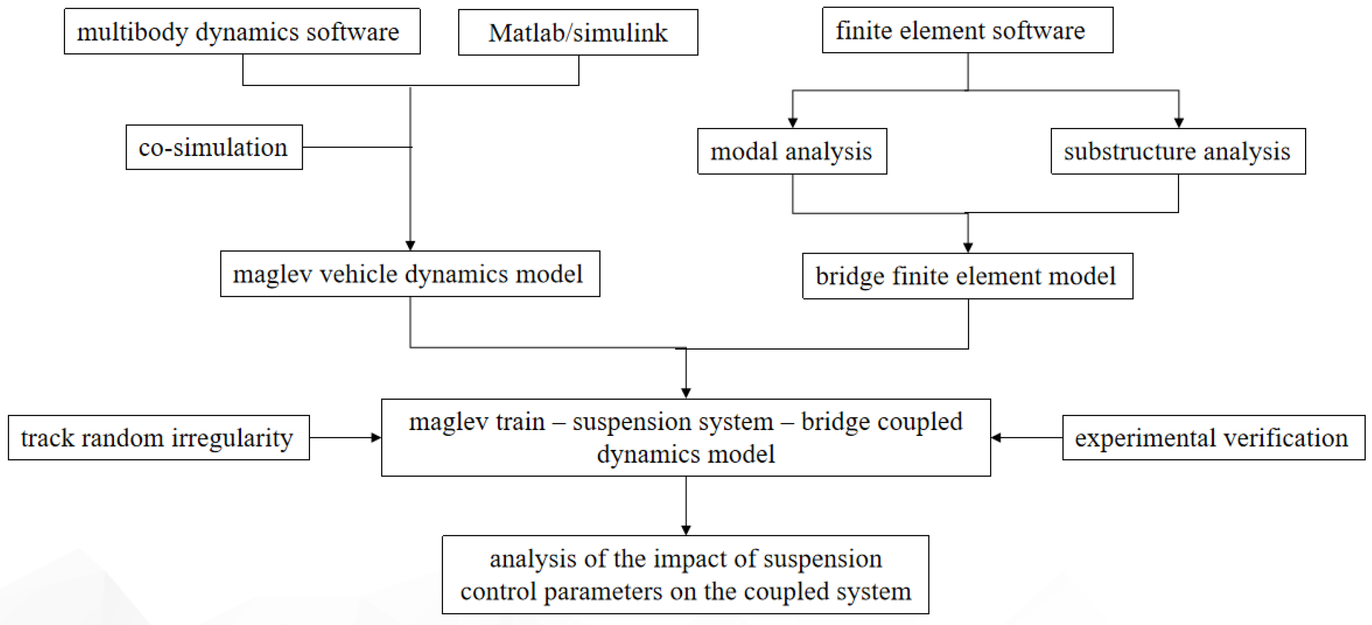
A suspension control system is established in Simulink and coupled with SIMPACK for co-simulation. The track’s random irregularities are introduced into the maglev vehicle dynamics model through external excitation. Ultimately, a coupled dynamic model of the maglev vehicle, suspension system, and bridge is developed, as shown in Figure 7.

The coupled dynamic model of the maglev vehicle, suspension system, and bridge established is shown in Figure 8. A total of three simply supported beam spans are set up 100 m ahead of the maglev vehicle model. Semi-rigid regions are established before and after the simply supported beams as buffer zones. A rigid region is set between the maglev vehicle and the flexible bridge. In the rigid region, the displacement, velocity, and acceleration at the nodes are all set to zero.

7. Model Validation

During the operation of the Qingyuan Maglev Tourist Line, extensive on-site testing was conducted. Vertical acceleration data related to the train body, suspension frame, and bridge span were collected when the train ran at 100 km/h on a straight section, and these results were compared with simulation calculations to verify the accuracy of the model.

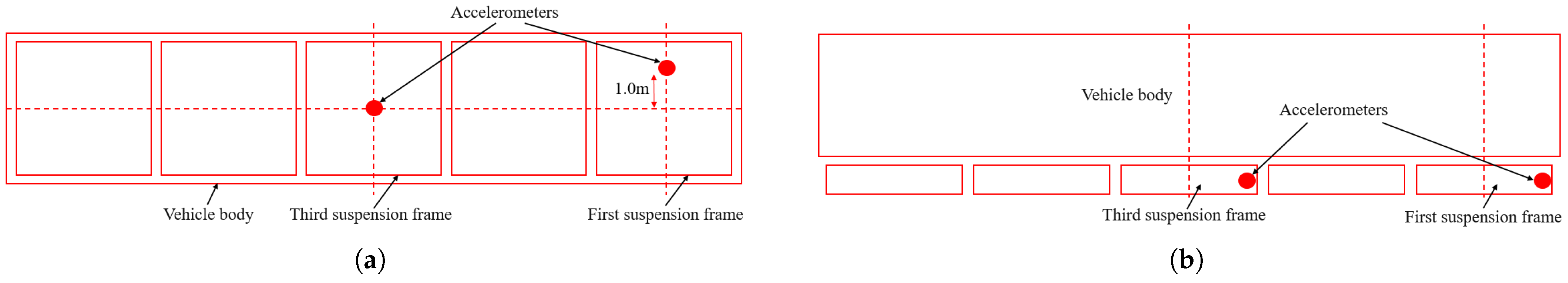
The data acquisition instrument used for the tests was the networked distributed acquisition and analysis instrument from the Beijing Oriental Vibration and Noise Technology Research Institute. The accelerometer sensors selected were the 991B type vibration sensor and the Dytran 3145A piezoelectric accelerometer. The arrangement of the accelerometers on the vehicle is shown in Figure 9, while the accelerometers on the bridge were placed at the mid-span of the beam.

As shown in Figure 10, the amplitude of the vertical acceleration of the vehicle body measured in the tests is relatively close to the simulation results, with the main vibration frequencies of the vehicle body being quite similar. The measured main vibration frequency of the vehicle body is 1.67 Hz, while the simulation result is 1.25 Hz. The test results contain more high-frequency components, mainly because the simulation model is a multi-rigid-body dynamics model, which only includes the rigid body motion of the vehicle body, whereas the actual measurements include some elastic deformation of the vehicle body and local high-frequency vibrations.

From Figure 11, it can be seen that the measured and simulated vertical acceleration of the suspension frame show minimal difference, with their main vibration frequencies being close. The measured results of the suspension frame have a more diverse frequency range.

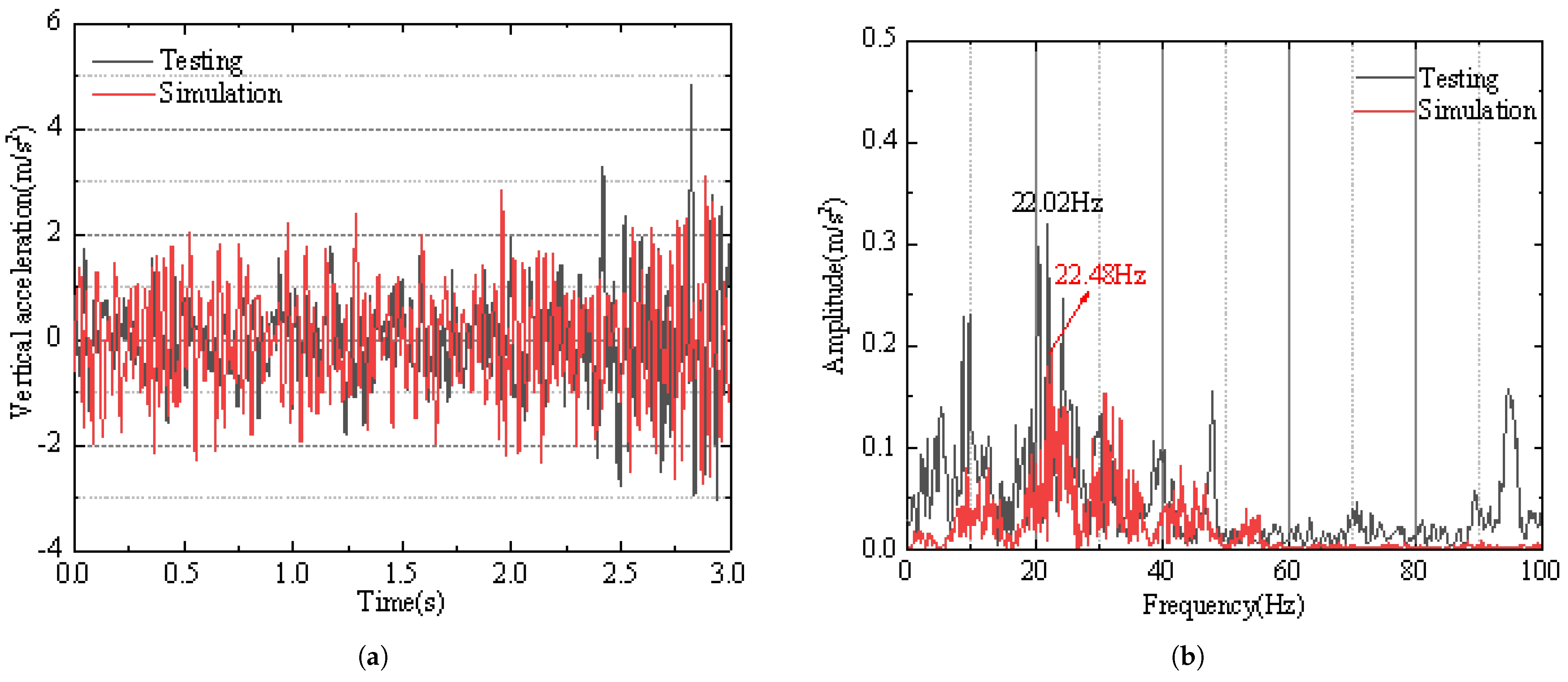
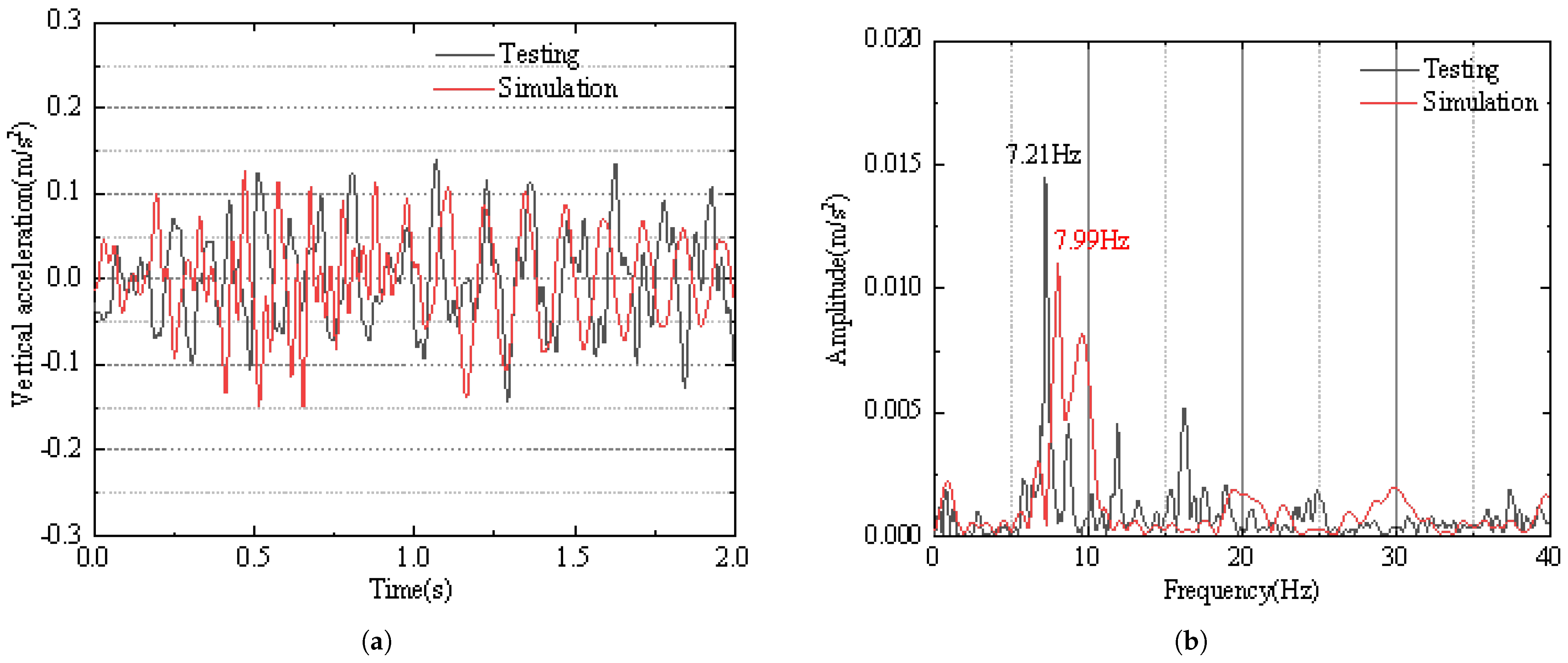
Figure 12 shows a comparison between the test and simulation results for the bridge. It can be observed that the vibration amplitudes of the two are quite similar. The measured main vibration frequency of the bridge is 7.21 Hz, while the simulation result is 7.99 Hz. Both frequencies are close to the first vertical bending mode frequency of the bridge, which is 7.47 Hz.

The comparison between the test and simulation results in this section verifies the accuracy of the mid–low-speed maglev vehicle–bridge coupling dynamic model established earlier in the paper.

8. Analysis of the Impact of Suspension Control Parameters on the Coupled System

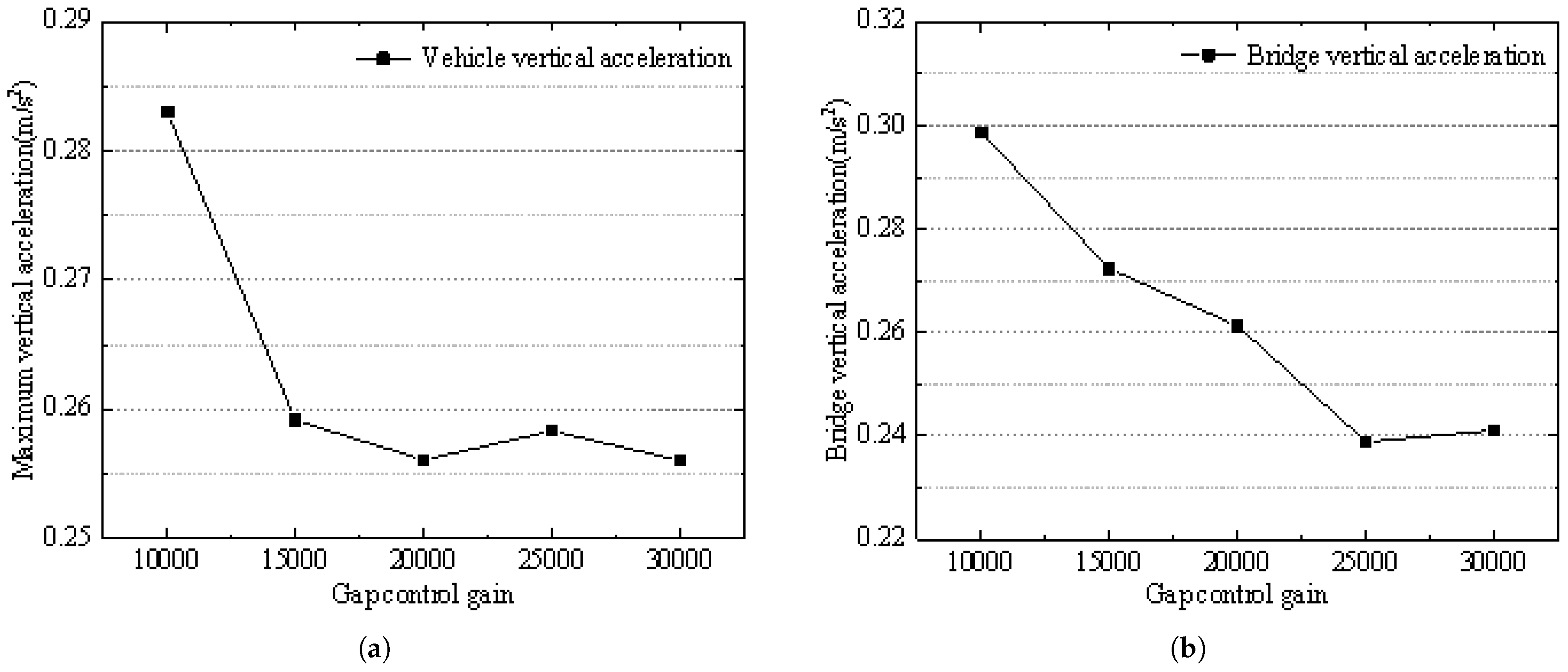
Using the maglev vehicle–suspension system–bridge coupling dynamic model established earlier, an analysis is conducted on the impact of suspension control parameters on the coupled system. Simulation calculations are performed for the dynamic responses of the vehicle, bridge, and suspension system. The vehicle speed is set to 80 km/h, with the gap control gain $k_p$ ranging from 10,000 to 30,000, and the gap velocity control gain $k_i$ ranging from 30 to 70.

As shown in Figure 13 and Figure 14, with the increase in the gap control gain, the vertical acceleration of the vehicle body first decreases and then fluctuates around 0.258 m/s². The vertical acceleration of the bridge shows a gradually decreasing trend, from 0.3 m/s² to 0.24 m/s². The fluctuation of the vehicle’s suspension gap shows a gradual decrease, from 0.376 mm to 0.178 mm.

In the maglev train’s suspension control system, the gap control gain $k_p$ reflects the “stiffness” of the electromagnetic suspension. When other control parameters remain constant, the larger the value of $k_p$, the greater the system’s suspension “stiffness”. In this case, the electromagnetic force’s response speed is faster, the adjustment speed of the suspension gap is improved, and the fluctuation of the suspension gap decreases.

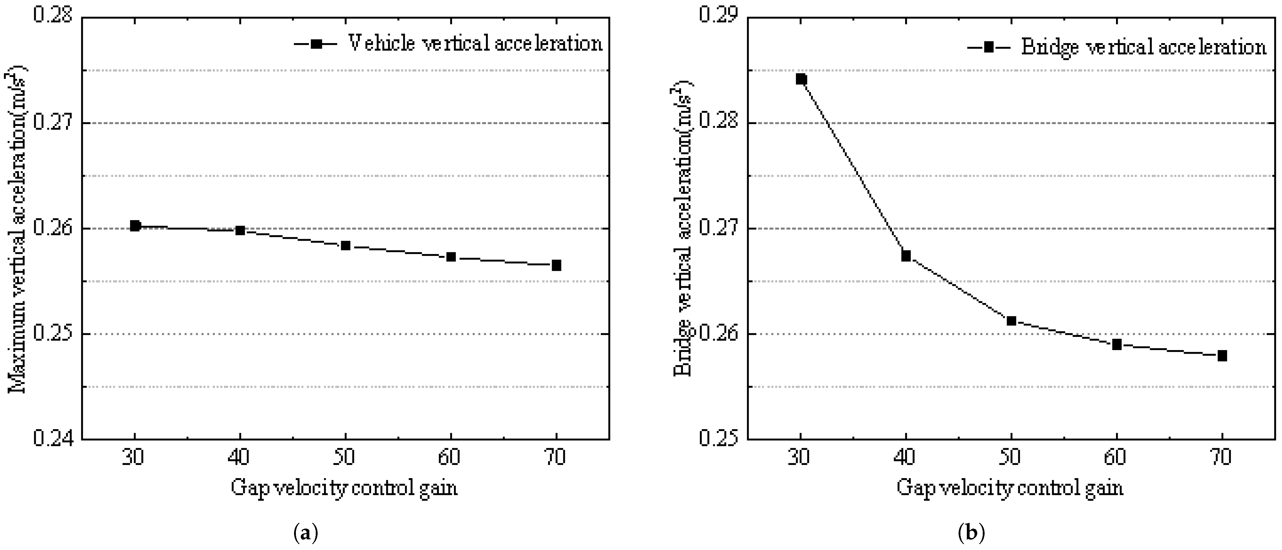
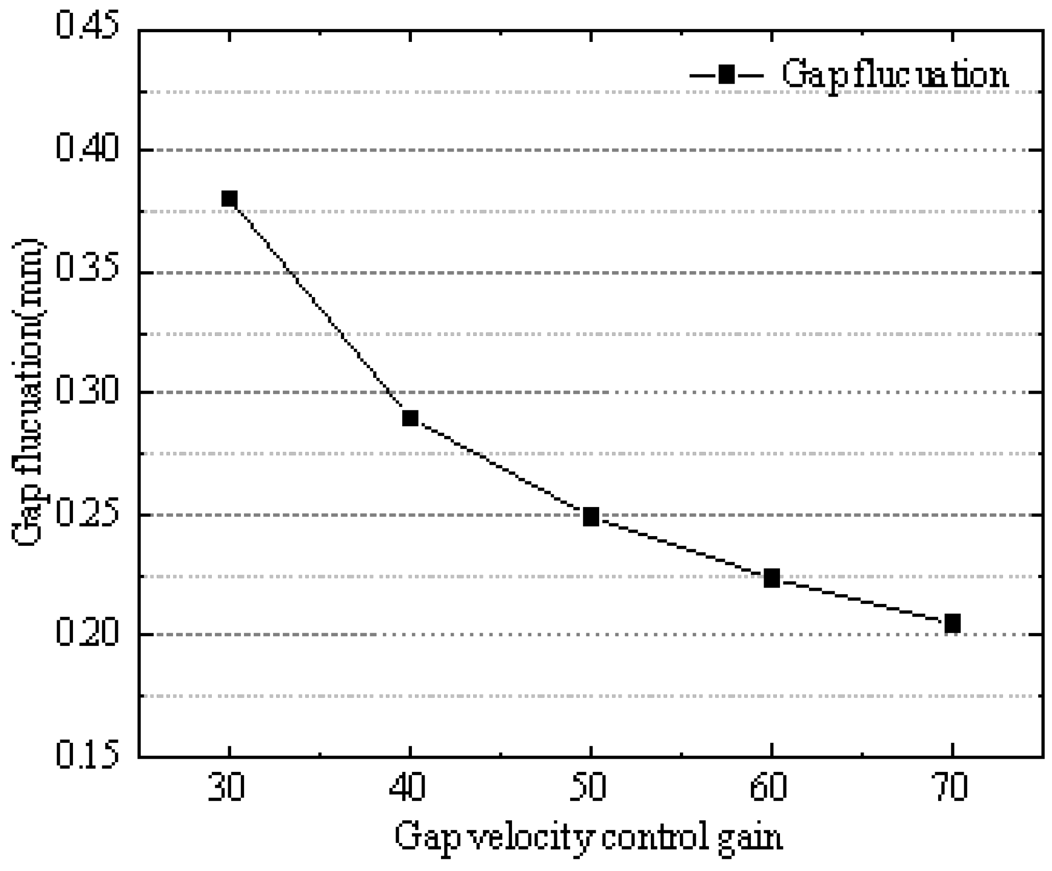
From Figure 15 and Figure 16, it can be seen that the vertical acceleration of the vehicle body slightly decreases as the gap velocity control gain increases. The vertical acceleration of the bridge decreases gradually with the increase in the gap velocity control gain, from 0.284 m/s² to 0.258 m/s². The fluctuation of the suspension gap decreases as the gap velocity control gain increases from 0.38 mm to 0.205 mm.

In the maglev train’s suspension control system, the gap velocity control gain acts as the system’s “damping”. Properly increasing the suspension system’s “damping” helps reduce oscillations, and the fluctuation of the suspension gap gradually decreases.

From the simulation results, it can be concluded that selecting appropriate suspension control parameters can effectively reduce the coupled vibration response between the maglev vehicle and the bridge, decrease the fluctuation of the suspension gap, and minimize the vibrations of the vehicle and bridge.

9. Conclusions

Based on the parameters of the mid–low-speed maglev vehicle and bridge structure of the Qingyuan Maglev Tourist Line, this paper establishes a multi-rigid-body vehicle dynamics model and a bridge finite element model. A mid–low-speed maglev vehicle–control system–bridge coupling dynamic model is then developed using the modal reduction method. The field-measured vibration data of the vehicle and bridge from the Qingyuan Maglev Tourist Line are compared with the simulation model results to verify the accuracy of the model established in this paper. Finally, the influence of suspension control parameters on the coupled system is analyzed. The calculation results show that selecting appropriate suspension control parameters can effectively reduce the coupled vibration response between the maglev vehicle and the bridge.