Article

Route-Preview Adaptive Model Predictive Motion Cueing for Driving Simulators

School of Mechanical Engineering, Yanshan University, Qinhuangdao 066000, China
*
Author to whom correspondence should be addressed.
Actuators 2025, 14(12), 588; https://doi.org/10.3390/act14120588 (registering DOI)
Submission received: 20 October 2025 / Revised: 22 November 2025 / Accepted: 26 November 2025 / Published: 2 December 2025
(This article belongs to the Section Actuators for Surface Vehicles)

Abstract

Motion cueing algorithm (MCA) aims to reproduce the dynamic motion experience of real vehicles for users of driving simulators. Under rough or irregular road conditions, vehicles are subjected to severe shocks and vibrations. However, due to the inherent response delay and limited capability of motion platforms in reproducing high-frequency components, conventional MCA often suffers from slow response and poor tracking accuracy. This mismatch leads to dynamic inconsistency between the visual feedback and the motion cues provided to the driver, which can easily induce discomfort or even aggravate simulator sickness. To address these issues, this study proposes a route-preview MCA based on adaptive model predictive control (RPAMPC). A CNN–LSTM-based vehicle trajectory prediction model is developed by integrating convolutional and recurrent neural networks to exploit forward terrain information. Subsequently, a motion cueing prediction model incorporating actuator stroke and velocity states is formulated, and an AMPC-based MCA is designed to optimize the simulator platform motion under physical constraints. Experimental results on a Stewart motion simulation platform demonstrate that, compared with traditional MCA, the proposed algorithm achieves higher-quality motion cues and significantly reduces sensory errors under complex road conditions.

1. Introduction

Vehicle driving simulators can be categorized into two types based on their functions: training-based and research-based simulators [1,2]. Training-based driving simulators primarily replicate complex driving scenarios, such as adverse weather conditions and emergency events, within virtual environments. Their primary objective is to enhance drivers’ skills and emergency response capabilities, thereby reducing operational errors, mitigating driving risks, and minimizing time and costs associated with training. In contrast, research-based driving simulators are primarily used to test and evaluate vehicle comfort and safety within driving simulation environments, aiming to optimize vehicle design and performance [3,4]. Owing to their significant practical value in both research and application, vehicle driving simulators have become indispensable tools for numerous leading automobile manufacturers.
To enhance the similarity between a simulator’s driving experience and that of a real vehicle, the visual, audio, and motion simulation systems must work in unison [5,6]. In this process, motion cueing algorithms utilize the limited space of the motion simulation platform to deliver a continuous and realistic motion experience for drivers, which is essential for achieving realistic kinetic simulation [7,8,9].
Extensive research has been conducted on MCAs by numerous scholars. In early studies, Conrad et al. [10] proposed the classic washout algorithm. This algorithm separates vehicle signals into high-frequency and low-frequency components using filters. High-frequency signals are simulated through the platform’s linear acceleration, whereas low-frequency signals are reproduced by tilting the platform at angular velocities below the human perception threshold, utilizing gravitational acceleration components. Although the classic washout algorithm features a simple structure and is easy to design, its fixed filtering parameters lead to conservative platform motion and suboptimal motion cueing quality. To address these limitations, researchers [11,12,13,14] have developed adaptive, fuzzy, and fuzzy neural network motion cueing algorithms to enhance the flexibility of filtering parameters. However, as these algorithms fail to account for the workspace limitations of the motion simulation platform in the planning process, improvements in motion cueing quality remain constrained.
In recent years, model predictive control (MPC) has become a research focus in the field of MCAs due to its superior capability for handling system constraints. Numerous studies have combined MCA with MPC and its advanced variants, significantly improving the motion cueing performance of driving simulators. For example. Dagdelen et al. [15] integrated the vestibular system and the workspace of the motion simulation platform to propose an MPC-based MCA. Their research demonstrates that MPC-based motion cueing algorithms effectively adjust input signals to the simulation platform, improving driving perception accuracy and maximizing workspace utilization. Qazani [16] introduced a linear time-varying MPC-based MCA that includes actuator stroke in trajectory planning, achieving more stable and precise control across diverse driving conditions and thereby improving adaptability and trajectory planning efficiency compared to traditional MPC-based approaches. Additionally, Qazani [17] introduced an adaptive MCA integrating fuzzy logic control with MPC for dynamic filter parameter adjustment. Simulation results indicate that this algorithm significantly improves motion cueing quality, optimizes workspace utilization, and reduces motion perception errors. Asadi [18] introduced a decoupled MPC-based MCA that independently controls the tilt and rotational channels. This approach improves response speed and control precision of the motion simulation platform in complex motion scenarios. Simulation results demonstrate that the decoupling method significantly improves motion cueing accuracy and reduces perceptual errors. Biemelt [19] proposed an online reference prediction strategy for MPC-based MCAs. This method incorporates a virtual driver model and a simplified vehicle dynamics model to predict driver inputs and the vehicle’s future trajectory, thereby enhancing MPC performance. Simulation results indicate that, compared to traditional constant reference trajectories, this strategy achieves better control of driving simulator motion, providing a more precise simulation experience. Lamprecht [20] developed an online MPC-based MCA that models the driver as an optimal controller and predicts steering behavior based on road geometry for reference trajectory updates. Experimental results confirm that this online MPC approach significantly enhances driving simulator immersion, particularly during steering scenarios.
Despite significant advancements in MCAs, several challenges and unresolved issues persist. First, most existing MCA studies primarily focus on flat or regular road conditions, with limited emphasis on motion cueing under complex road scenarios. In harsh road environments, vehicles frequently experience significant shocks and intense vibrations, resulting in response delays and reduced tracking accuracy in motion simulation platforms. Second, although current MCAs consider actuator stroke in the motion planning of simulation platforms, they frequently overlook actuator velocity constraints. The motion of the simulation platform is restricted by both actuator stroke limits and velocity boundaries, which must both be incorporated to improve motion cueing accuracy and responsiveness.
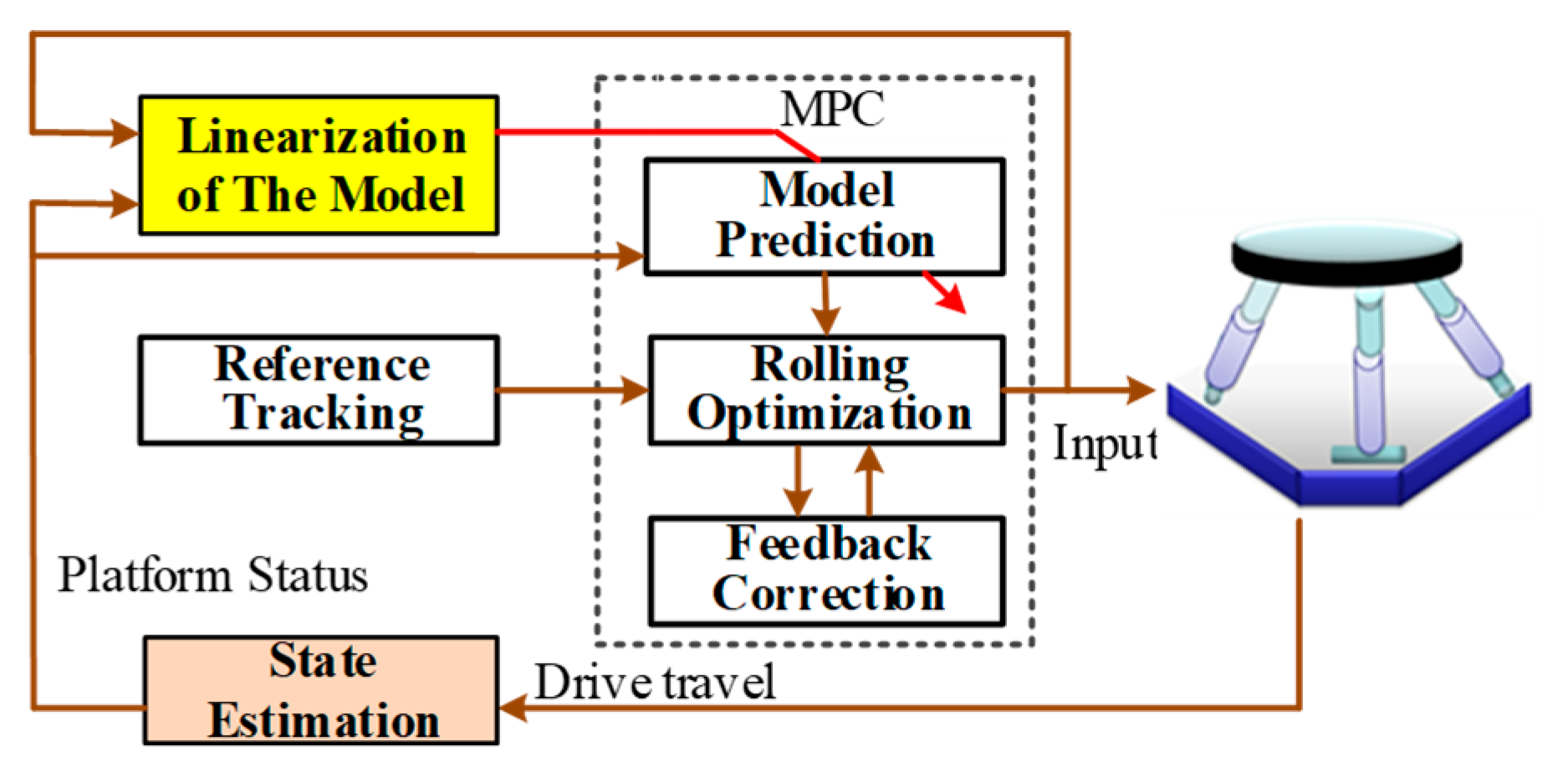
To address these challenges, this paper introduces an MCA based on AMPC with route preview. The overall control framework is illustrated in Figure 1. Specifically, a data-driven prediction model is developed to leverage front road terrain and vehicle state information for predicting the vehicle’s future trajectory, while adaptive model predictive control is employed to compute the optimal motion trajectory for the motion simulation platform. The primary contributions of this study are summarized as follows:
(1)
A route-preview vehicle trajectory prediction framework is presented, in which forward terrain elevation maps are utilized as inputs to a CNN–LSTM deep network. By learning the nonlinear interactions among terrain features, vehicle dynamics, and driver operations, the network enables short-horizon prediction of future vehicle attitudes and accelerations under highly irregular road conditions.
(2)
A motion cueing prediction model is formulated, within which actuator stroke and velocity states are explicitly incorporated. Through the introduction of a dynamics-based platform model and the embedding of actuator stroke and velocity constraints into the prediction process, the physical feasibility of both reference trajectories and control solutions is ensured, thus addressing a key limitation of traditional MCA approaches that neglect actuator-level physical constraints.
(3)
An AMPC motion cueing algorithm integrated with EKF-based state estimation is developed, whereby real-time, filtered platform states are provided to enhance the consistency between the predictive model and the actual system dynamics. This integration enables a closed-loop prediction–estimation–optimization structure, leading to improved robustness and tracking performance under complex road excitations.
The structure of this paper is as follows: Section 2 introduces the dynamic vehicle trajectory prediction model utilizing front road terrain. Section 3 elaborates on the MCA based on AMPC. Section 4 evaluates the proposed algorithm’s performance under diverse road conditions. The conclusions are detailed in Section 5.

2. Vehicle Trajectory Prediction Model

The early forecasting of the vehicle trajectory constitutes a fundamental requirement for enhancing the platform’s response speed and the overall quality of motion cueing. This paper employs deep learning to predict future vehicle trajectories. This approach is driven by two primary factors. First, the mathematical modeling of interactions between wheels and complex terrains is highly intricate, making it challenging to derive analytically. Second, neural network-based prediction methods eliminate the need for explicit modeling and can effectively capture and forecast these dynamic relationships. This section proposes a vehicle trajectory prediction algorithm based on CNN-LSTM.

2.1. Definition of Inputs and Outputs

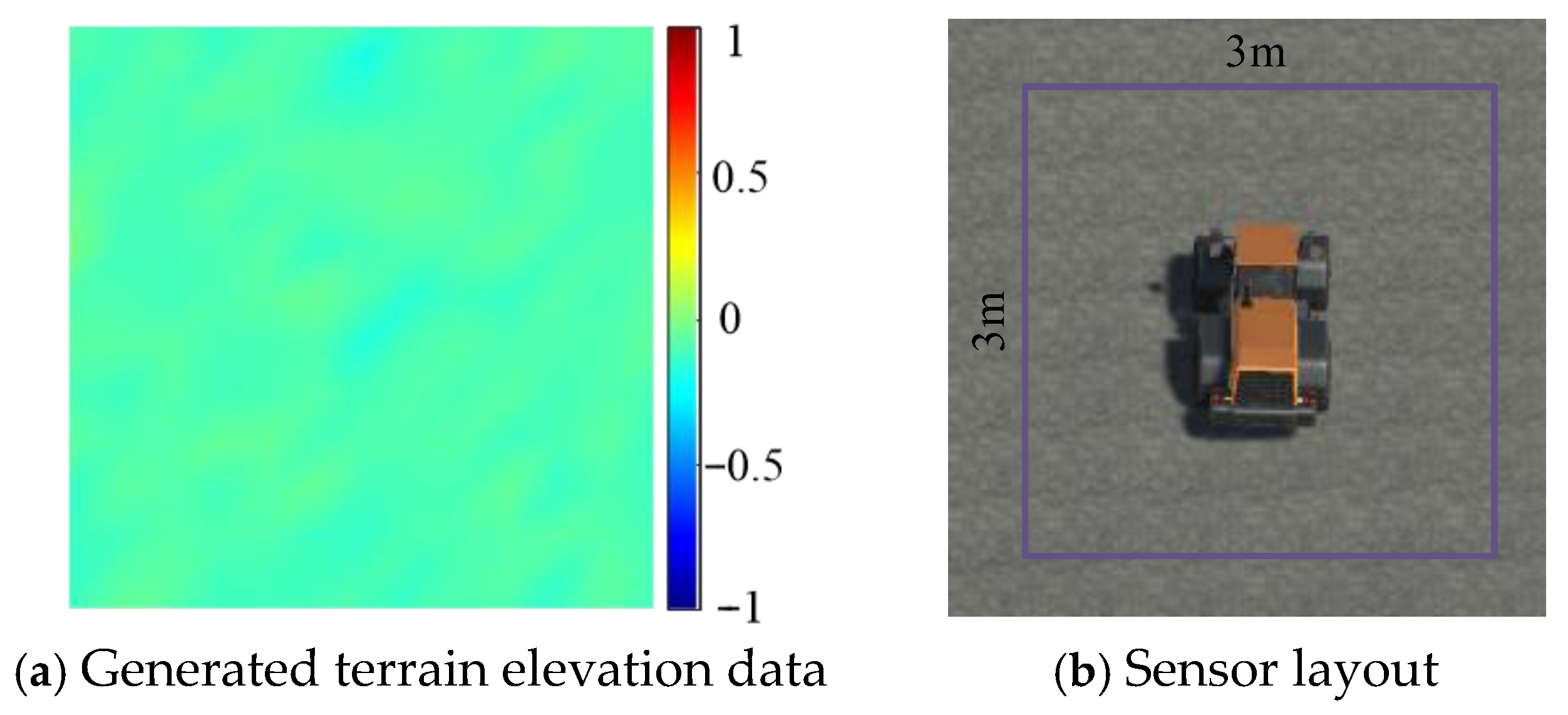
The future trajectory of a vehicle is primarily influenced by the road conditions ahead, the vehicle’s state, and the driver’s actions. In this study, the PhysX engine is used to simulate vehicle dynamics, and virtual sensors (Raycast) provided by Unity are employed to capture the terrain elevation map ahead of the vehicle, as shown in Figure 2.
For road condition information, the state of the road condition at any time t is represented as
s t R = [ r i j ] ( i = 1 , 2 30   ; j = 1 , 2 30 )
where rij is the height map of the terrain ahead of the vehicle, obtained using the onboard sensor, with an area size of 3 × 3 and a pixel size of 30 × 30 .
The vehicle state at any time t can be expressed as
s t V = [ v ¯ x , v ¯ y , v ¯ z , a ¯ x , a ¯ y , a ¯ z , w ¯ x , w ¯ y , w ¯ z ]
where v ¯ x , v ¯ y , v ¯ z , a ¯ x , a ¯ y , a ¯ z , w ¯ x , w ¯ y , w ¯ z is the vehicle’s velocity, acceleration, and angular velocity in the three respective directions.
Since the vehicle generally does not experience frequent acceleration or braking during operation, using the current pedal position at the predicted time as input provides a highly accurate approximation of the driver’s actual input within the short-term prediction interval. Therefore, at any time t, the driver’s state can be represented as
s t H = [ α a c c , α d e c , α s t e ]
where α a c c , α d e c , α s t e is the throttle, brake, and steering wheel inputs, respectively.
Define the road condition, vehicle status, and driving operation status in front of the vehicle at any given time t as xt, and represent its time series Xin as the input to the neural network, as follows:
x t = [ s t R , s t V , s t H ]
X i n = x t t h , x t t h + 1 , x t 1 , x t
where x t = [ s t R , s t V , s t H ] , th denotes the length of historical data.
Define the acceleration and angular velocity of the vehicle as y, and represent its future time series Yout as the output of the neural network, as follows
y t = [ a ¯ x , a ¯ y , a ¯ z , w ¯ x , w ¯ y , w ¯ z ]
Y o u t = y t , y t + 1 , y t + p 1 , y t + p
where tp denotes the prediction length.

2.2. Driving Scenarios Creation

In driving simulators, the road model serves not only as a medium for vehicle motion but also as a stimulus inducing changes in vehicle attitude. The surface contour characteristics of the road are typically described by road roughness, which is represented by power spectral density in the frequency domain. According to the ISO/DIS 8608 and GB7031-86 standards [21,22], roads are classified into eight categories based on the road roughness, as outlined in Table 1.
The power spectral density of road roughness is generally expressed as
G d ( n ) = G d ( n 0 ) ( n n 0 ) w
where n 0 represents the reference spatial frequency, typically set to n 0 = 0.1 m−1, and w is the frequency exponent of the power spectral density, usually set to w = 2.
Within the spatial frequency range n1 < n < n2, the variance σ d 2 of road roughness can be expressed as
σ d 2 = n 1 n 2 G d ( n ) d n
where the wavelength that affects vehicle motion state and driving comfort corresponds to a spatial frequency distribution of 0.011 m − 1 < n < 2.83 m − 1.
Furthermore, by discretizing the selected spatial frequencies into m small intervals of width Δ n i , the variance of road roughness is obtained by taking the central spatial frequency of each interval, G d ( n m i d , i ) , as the representative value.
σ d 2 = i = 1 m G d ( n m i d , i ) Δ n i
The three-dimensional modeling of random road surfaces is achievable using various methods [23], including white noise, harmonic superposition, and inverse Fourier transform methods. This paper utilizes the harmonic superposition method to model the road surface, where the roughness model of the random road surface is derived by superimposing sine functions over m small intervals, as follows:
q ( x , y ) = i = 1 m 2 G d ( n m i d , i ) Δ n i sin ( 2 π n m i d , i x + θ i ( x , y ) )
where θ i is a random number belonging to the interval 0 , 2 π .
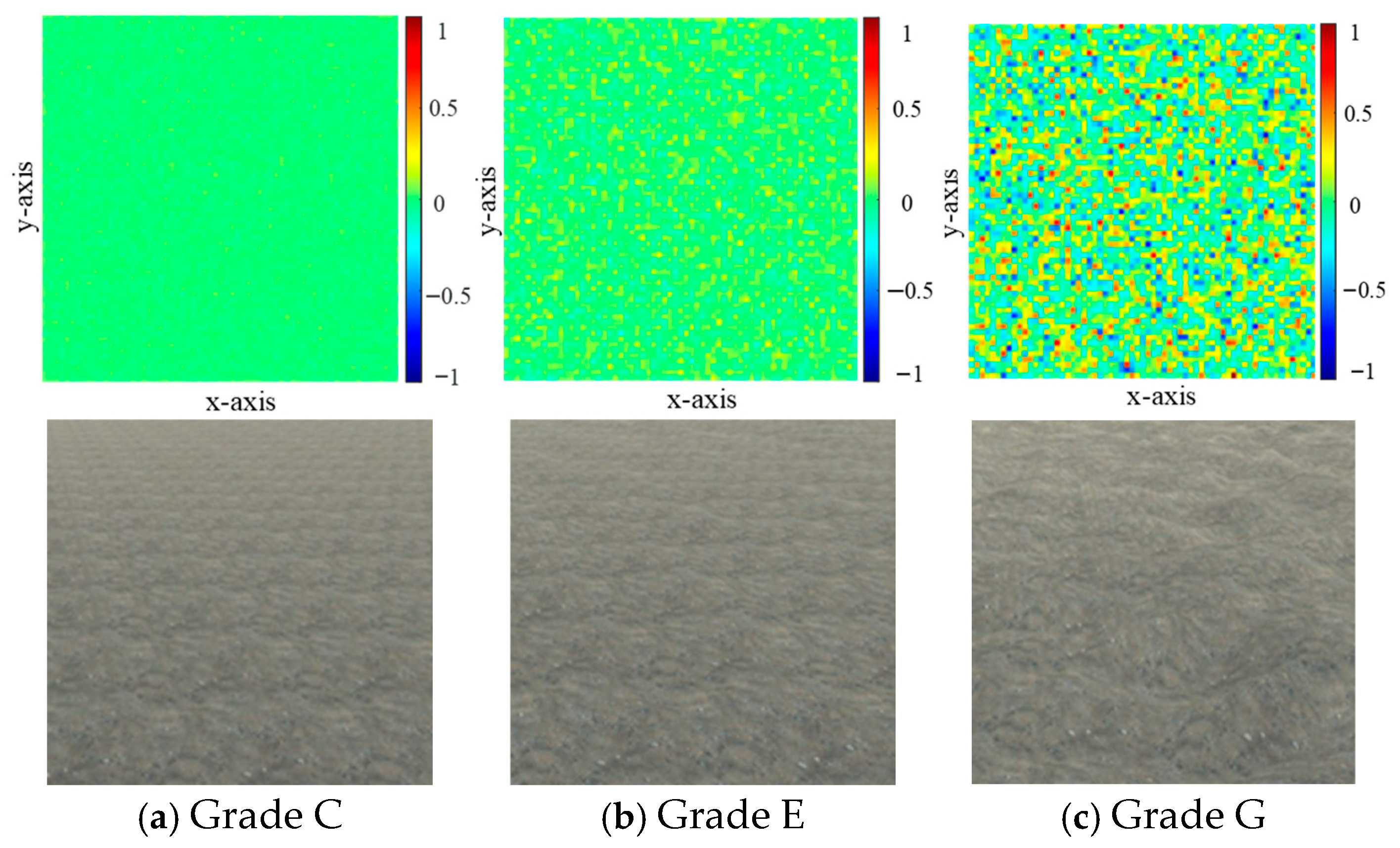
According to Equation (9), elevation maps for three different road surface grades, C, E, and G, are generated within a 129 m × 129 m region. These generated elevation maps are then imported into Unity to create the corresponding road surfaces, as shown in Figure 3. Subsequently, the driver is permitted to operate the vehicle randomly on roads of varying grades. Throughout the driving process, information such as the elevation map in front of the vehicle, the vehicle’s state, and the driver’s operations is recorded. A total of 15,211, 24,148, and 28,250 time series are collected for terrain grades C, E, and G, respectively.

2.3. Architecture and Evaluation of Networks

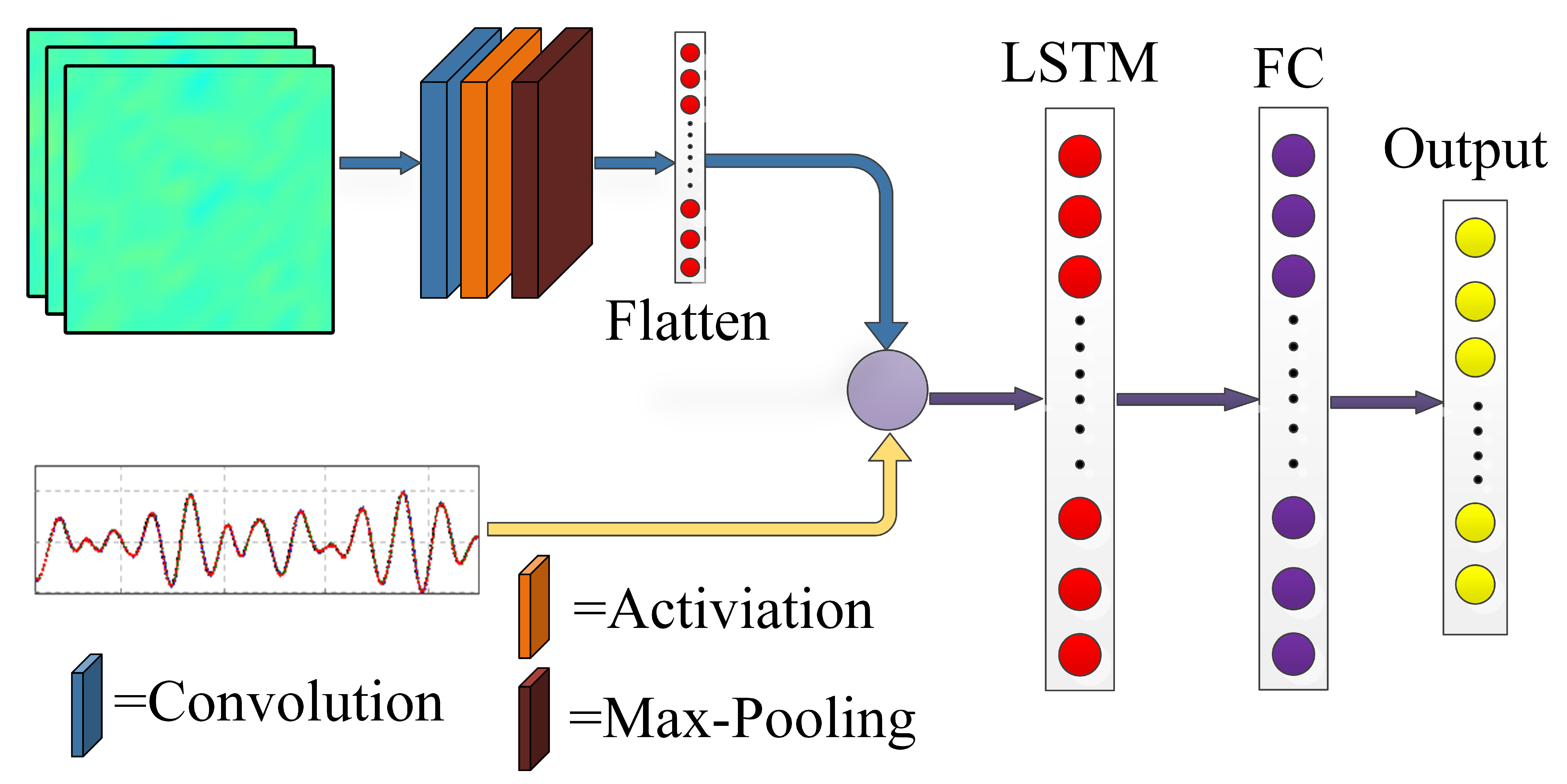
To comprehensively account for both temporal and spatial features in vehicle trajectory prediction and to enhance the robustness and generalization capability of the prediction algorithm, we propose a vehicle trajectory prediction algorithm based on CNN-LSTM. The approach involves extracting spatial features from the elevation map using a CNN and integrating them with temporal signals, including vehicle states, decomposed elevation information, and driver operations. Subsequently, an LSTM network is employed to effectively capture temporal features, thereby improving the overall performance of vehicle trajectory prediction.
The proposed CNN-LSTM architecture is illustrated in Figure 4. This architecture comprises a CNN component with convolutional layers, activation layers, pooling layers, and a flattening layer, followed by an LSTM component. Specifically, the convolutional layers utilize 16 filters of size 2 × 2, the activation layers employ ReLU activation, and the pooling layers have a size of 2 × 2. The output of the CNN component is flattened, combined with temporal signals, and further processed through the LSTM. The LSTM network consists of 200 units and employs stochastic gradient descent with momentum (SGDM) for optimization. In this paper, the sensor sampling period is set to 0.1 s, and the prediction horizon spans 15 time steps into the future, corresponding to tp = 1.5 s. Consequently, the size of the fully connected layer is configured to 90. For detailed specifications of the CNN and LSTM network units, please refer to the relevant literature [24,25].
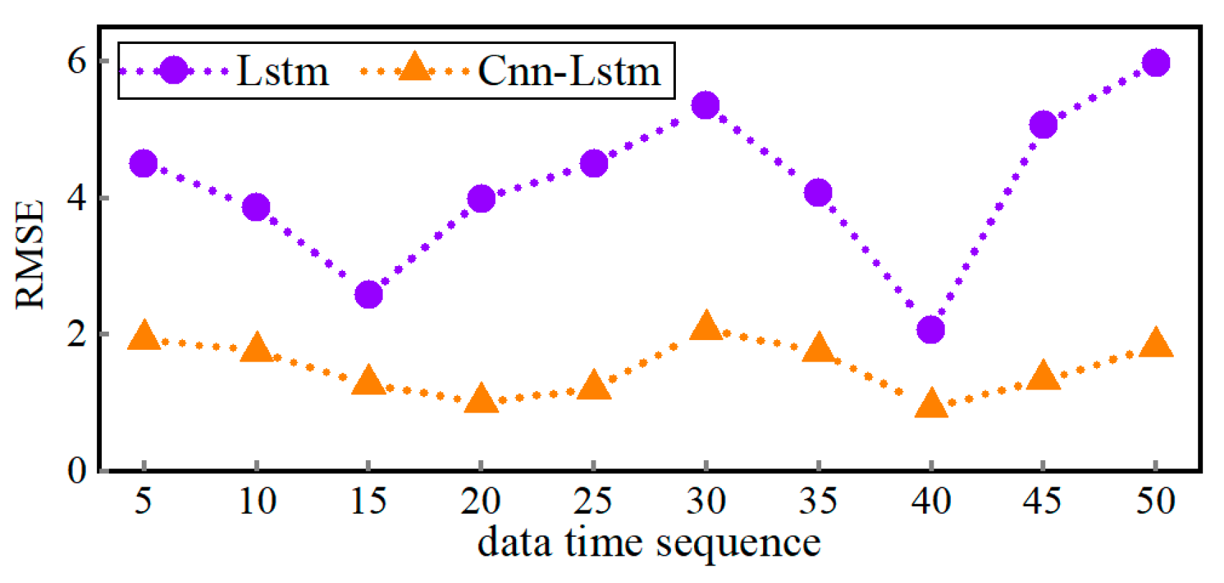
In order to achieve optimal prediction performance, the prediction accuracy of various approaches was compared, with the results shown in Figure 5. The CNN-LSTM-based vehicle trajectory prediction model outperforms the LSTM-based model in terms of predictive accuracy. Furthermore, Figure 5 depicts the prediction accuracy for forecasting the vehicle’s future 15 steps using time-series data of varying lengths. The results show that the smallest error is achieved when the vehicle’s future 15 steps are predicted using data from the past 20 steps. Therefore, in this paper, the value of th is defined as 20.

3. AMPC-Based MCA

In Section 2, a CNN–LSTM-based deep learning model is developed to predict the vehicle’s future accelerations and angular velocities using forward terrain information, vehicle states, and driver inputs, thereby providing feed-forward reference signals for the motion cueing algorithm. Building upon these predictions, this chapter further constructs an AMPC framework for the motion simulation platform. The predicted vehicle trajectory is used as the reference input, and the AMPC optimizes the platform’s motion trajectory and control inputs while simultaneously accounting for human vestibular perception characteristics and the actuator stroke and velocity constraints of the platform.

3.1. Motion Planning Model of the Platform

3.1.1. Human Vestibular System Model

As the human body is unable to effectively differentiate between gravitational and motion acceleration, the MCA simulates acceleration via coordinated tilting. In the driving simulator, the specific force f experienced by the driver is the sum of the platform’s linear acceleration and the gravitational components, as follows:
f T a x + g θ a y g ϕ a z g = a x + g 1 s 2 α y a y g 1 s 2 α x a z g
where a x , a y , a z denote the accelerations of the motion simulation platform in the longitudinal, lateral, and vertical directions, respectively. α x , α y are the angular accelerations of the longitudinal and lateral axes of the platform, respectively. f is the force experienced by the human body, and g is the gravitational acceleration.
According to Young, Ormsby et al. [26,27,28], the transfer function of the otolith model can be expressed as
f ^ f = k o t o ( τ a s + 1 ) ( τ L s + 1 ) ( τ s s + 1 )
The human body primarily relies on the semicircular canals to detect angular velocity. The transfer function between the detected angular velocity w ^ and the true angular velocity w can be expressed as
w ^ w = t 1 t b s 2 ( t 1 s + 1 ) ( t 2 s + 1 ) ( t b s + 1 )
Based on Equations (12)–(14), the state-space representation of the vestibular system is expressed as follows:
x ˙ V = A V x V + B V u y V = C V x V + D V u
where A V , B V , C V , D V , are the state-space matrices for the human vestibule, while a ^ x , a ^ y , a ^ z , w ^ x , w ^ y and w ^ z , are the specific forces and angular velocities perceived by the human body in the three directional axes.
u = ( α y a x α x a y α z a z ) T , A V = A O T O 0 0 A S C C ,   B V = B O T O B S C C , C V = C O T O 0 0 C S C C , D V = 0 , y V = a ^ x a ^ y a ^ z w ^ y w ^ x w ^ z T .

3.1.2. Motion Simulation Platform State Model

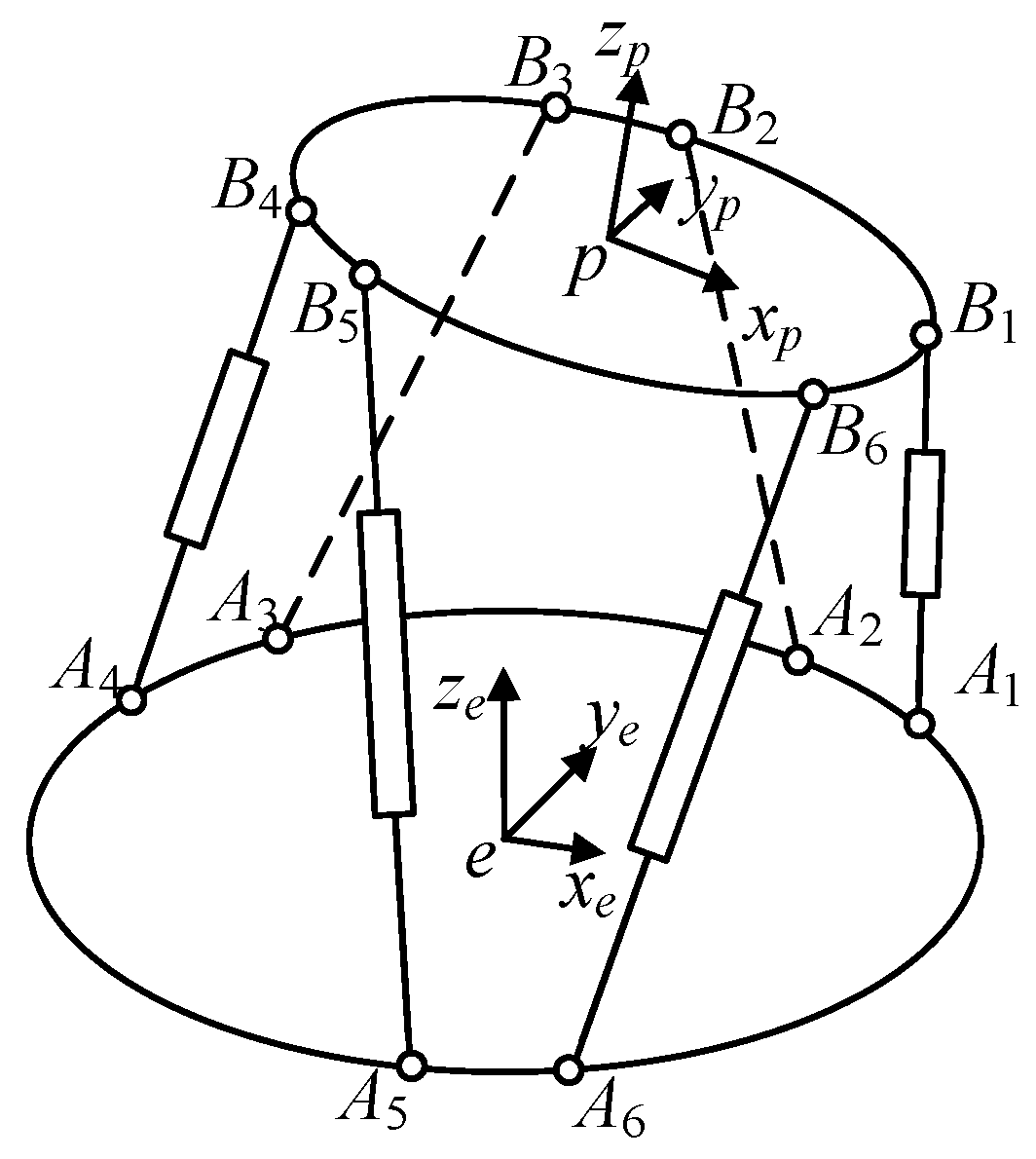
The motion simulation platform is a system with physical constraints, where the constrained variables are the stroke and velocity of the actuators. Therefore, it is necessary to establish a state-space equation that includes the stroke and velocity of the actuators to control the impact of inputs on the actuators. The structure of the motion simulation platform is shown in Figure 6. The state of the motion simulation platform can be expressed as follows:
x ˙ d = A d x d + B d u
where
A d = A       A       A ,   B d = B       B       B , A = 0 1 0 0 0 0 0 0 0 0 0 1 0 0 0 0 ,   B = 0 0 0 1 0 0 1 0 ,
x d = x v x θ y w y y v y θ x w x z v z θ z w z T ,
u = ( α y a x α x a y α z a z ) T .
where x , y , z , v x , v y , v z , θ x , θ y , θ z , w x , w y , w z represent the displacement, velocity, angles, and angular velocity of the motion simulation platform in three directions, respectively.
The length of the actuator rod can be further represented as
l i = s + R b i a i 2 ( i = 1 , 2 , , 6 )
where s = [x y z]T, bi = [xbi ybi zbi]T is a constant representing the position vector of point Bi in coordinate system p-xpypzp, and ai = [xai yai zai]T is a constant representing the position vector of point Ai in coordinate system e-xeyeze.
By squaring both sides of Equation (15) and differentiating with respect to time, the velocity expression for the actuator is derived.
l ˙ i = 1 l i M T N
where rij is the element of the rotation matrix R.
M = x + r 11 r 12 r 13 b i x a i y + r 21 r 22 r 23 b i y a i z + r 31 r 32 r 33 b i z a i , N = v x + r ˙ 11 r ˙ 12 r ˙ 13 b i v y + r ˙ 21 r ˙ 22 r ˙ 23 b i v z + r ˙ 31 r ˙ 32 r ˙ 33 b i .
Based on the principles of kinematics, the differentiation of the vector Rbi results in
( R b i ) = w × ( R b i )
where w = [wx wy wz]T.
According to Equations (18) and (19), the velocity of the actuator can be further expressed as
l ˙ i = n i T ( v + w × ( R b i ) ) = n i T v + n i T ( w × ( R b i ) )
where v = v x v y v z T .
n i = 1 l i x + r 11 r 12 r 13 b i x a i y + r 21 r 22 r 23 b i y a i z + r 31 r 32 r 33 b i z a i  
According to the mixed product property, Equation (20) can be reformulated as
l ˙ i = n i T v + n i T ( w × R b i ) = n i T v + ( R b i × n i ) T w
Equation (22) can be represented in matrix form as
l ˙ i = n 1 T ( R b 1 × n 1 ) T n 2 T ( R b 2 × n 2 ) T n 6 T ( R b 6 × n 6 ) T v w
Taking the derivative of Equation (23) produces the actuator acceleration
l ¨ i = = J ˙ v w + J a α
where J ˙ = n ˙ 1 T ( w × R b 1 × n 1 + R b 1 × n ˙ 1 ) T n ˙ 2 T ( w × R b 2 × n 2 + R b 2 × n ˙ 2 ) T n ˙ 6 T ( w × R b 6 × n 6 + R b 6 × n ˙ 6 ) T ,   J = n 1 T ( R b 1 × n 1 ) T n 2 T ( R b 2 × n 2 ) T n 6 T ( R b 6 × n 6 ) T .
Based on Equations (19) and (21), the expression for n ˙ i is derived as follows:
n ˙ i = 1 l i v x + r ˙ 11 r ˙ 12 r ˙ 13 b i v y + r ˙ 21 r ˙ 22 r ˙ 23 b i v z + r ˙ 31 r ˙ 32 r ˙ 33 b i = v + w × ( R b i ) l i
Furthermore, by combining (19) and (21), the state-space equation for velocity-based actuator planning can be derived as follows:
x ˙ L = A L x L + B L u
where
A L =           A d             0 0 J 11 0 J 14 0 J 12 0 J 15 0 J 13 0 J 16 0 0 J 61 0 J 64 0 J 62 0 J 65 0 J 63 0 J 66 0 0 J ˙ 11 0 J ˙ 14 0 J ˙ 12 0 J ˙ 15 0 J ˙ 13 0 J ˙ 16 0 0 J ˙ 61 0 J ˙ 64 0 J ˙ 62 0 J ˙ 65 0 J ˙ 63 0 J ˙ 66 0
B L =     B d           0 6 × 6       J 15 J 11 J 14 J 12 J 16 J 13 J 65 J 61 J 64 J 62 J 66 J 63 , x L = x d l 1 l 2 l 6 l ˙ 1 l ˙ 2 l ˙ 6 .
According to Equations (15) and (26), the trajectory planning model of the motion simulation platform is derived as follows:
x ˙ T = A T x T + B T u
where
A T = A V     A L ˙ ,   B T = B V B L ˙ , x T = x V x L T .
Since the Jacobian matrix depends on the instantaneous posture of the platform, and the platform posture continuously changes during the motion simulation process, the state-space model in (27) constitutes a linear parameter-varying (LPV) system.

3.2. Adaptive Model Predictive Control

AMPC consists of six components: state estimation, model linearization, model updating, rolling optimization, and feedback correction, as shown in Figure 7.

3.2.1. State Estimation

According to Equation (27), the trajectory planning model of the motion simulation platform is time-varying. To achieve online closed-loop control of the motion cueing algorithm, the state of the motion simulation platform must be acquired in real time. On the one hand, this state information is used for the time-varying linearization of the nonlinear motion planning model. On the other hand, it is utilized for feedback correction to optimize control outputs. This article proposes an online state estimation algorithm for motion simulation platforms based on EKF.
EKF is a state estimation method designed for nonlinear dynamic systems. This method processes data by linearizing the nonlinear system model at each time step and then applying the standard Kalman filtering algorithm. EKF comprises two main stages: prediction of the state and error covariance, and updating of the state and error covariance [28].
Prediction   x ^ k | k 1 = f ( x ^ k | k 1 , u k ) P k | k 1 = Φ k P k 1 | k 1 Φ k T + Q k
Update   K k = P k | k 1 H k T ( H k P k | k 1 H k T + R k ) 1 x ^ k | k = x ^ k | k 1 + K k ( z k H k x ^ k | k 1 ) P k | k = ( I n K k H k ) P k | k 1
where x ^ k | k 1 represents the a priori estimate of the state, and x ^ k | k represents the a posteriori estimate of the state. P k | k 1 denotes the a priori error covariance of the state, and P k | k denotes the a posteriori error covariance of the state. Φ k is the state transfer matrix, Q k is the process noise covariance, z k is the measurement value, H k is the measurement matrix, and R k is the measurement noise covariance. K k is the Kalman gain, and I is the unit matrix.
In the motion simulation platform, the stroke of the actuator can be directly measured by internal sensors; therefore,
z k = l 1 l 2 l 3 l 4 l 5 l 6 .

3.2.2. Model Predictive Control

MPC achieves optimal control by modeling and predicting the system’s behavior. It solves an optimization problem at each control cycle, determining the optimal sequence of control inputs to achieve the desired control objectives.
To obtain the prediction model, the state-space (27) needs to be discretized.
x ˙ d ( k + 1 ) = A d x d ( k ) + B d u d ( k ) y ( k ) = C d x d ( k )
To eliminate the discrepancy between the predicted model and the actual system, an integral term is introduced to obtain the augmented state-space model.
x ˙ ( k + 1 ) = A x ( k ) + B Δ u ( t ) y ( k ) = C x ( k )
where
x ( k ) = Δ x d ( k ) T y ( k ) T , Δ x d ( k ) = x d ( k ) x d ( k 1 ) ,
A = A d 0 C d A d I   , B = B d C d B d   , C = 0 I .
Through recursion, the extended state-space equation is expanded to the state equation with a prediction horizon Np and control horizon Nc as follows:
Y ( k ) = F x ( k ) + Φ Δ U
where Y ( k ) = y ( k + 1 ) y ( k + 2 ) y ( k + N p ) T ,
Δ U ( k ) = u ( k ) u ( k + 1 ) y ( k + N c 1 ) T .
The control objective of the motion simulation platform is to enable the platform to track the reference signal R(k) with high precision at each sampling moment k, while ensuring the platform operates within its physical constraints. Therefore, the objective function is set as
min J = i = 1 N p 1 ( R s ( k ) Y ( k ) ) T Q ( R s ( k ) + Y ( k ) )   + i = 1 N c 1 U ( k ) T S U ( k ) + i = 1 N c 1 Δ U ( k ) T R Δ U ( k )
s . t U min U ( k ) U max Δ U min Δ U ( k ) Δ U max Y min Y ( k ) Y max
where Q, S, and R are the diagonal weighting matrices corresponding to the output, input, and input rate, respectively. Umin and Umax are the lower and upper limits of the input, respectively, and △Umin and △Umax are the lower and upper limits of the input rate. Ymin and Ymax are the lower and upper limits of the output.

3.3. Objective Evaluation

The objective evaluation of motion cueing quality forms the basis for their parameter tuning, assessment, and comparison. The commonly used objective metrics for evaluating motion cueing quality include (1) the correlation coefficient (CC) and (2) the root mean square error (RMSE).
CC ( x , y ) = i = 1 n ( x i x ¯ ) ( y i y ¯ ) i = 1 n ( x i x ¯ ) 2 i = 1 n ( y i y ¯ ) 2
where
  x ¯ = 1 n . i = 1 n x i             y ¯ = 1 n . i = 1 n y i
RMSE ( x , y ) = i = 1 n ( x i y i ) 2 n

4. Results and Discussions

4.1. Design of the Experimental Scheme

Upon completion of the AMPC-based MCA, the control system was simulated in MATLAB, with continuous calibration of the controller parameters. Following the debugging phase of the control system, a closed-loop test for vehicle motion cueing based on route preview was conducted.
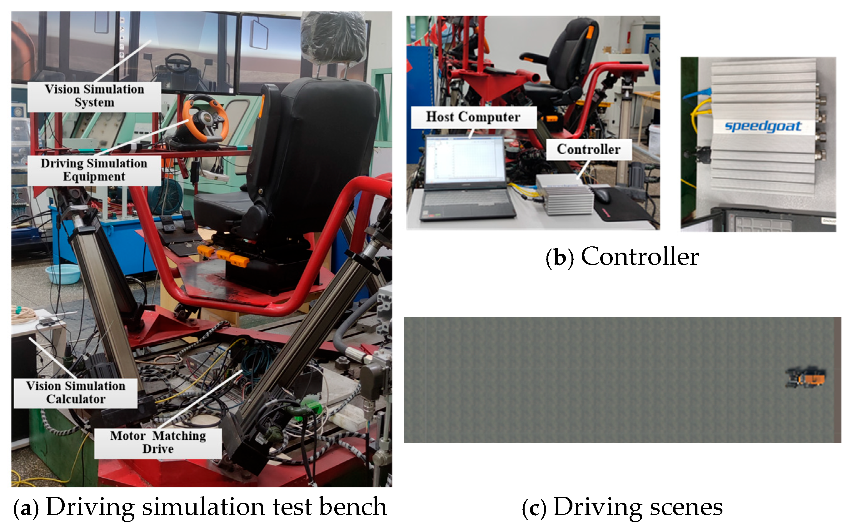
As shown in Figure 8, the driving simulator consists of a visual simulation system, a driving cockpit, a visual simulation computer, a controller, and a motion simulation platform equipped with six electric actuators and their corresponding drivers. Each actuator has a maximum stroke of 0.4 m, a maximum velocity of 0.4 m/s, and a maximum acceleration of 5 m/s2. The simulator controller adopts the basic version of the real-time target machine developed by Speedgoat, which provides seamless integration with MATLAB/Simulink (2021). The real-time target machine is equipped with an Intel Celeron 2 GHz quad-core processor, a 64 GB SSD, and 4 GB RAM, ensuring stable and efficient real-time computation.
To ensure a fair comparison of motion cueing quality across different algorithms, the following procedure was adopted: First, the driver operates the vehicle in a complex road scenario, during which vehicle states and other parameters are recorded and stored in a time-series database. Subsequently, the time-series data is used as input for various algorithmic solutions within the control system, enabling an objective evaluation of the vehicle’s motion perception quality.

4.2. Experimental Results and Analysis

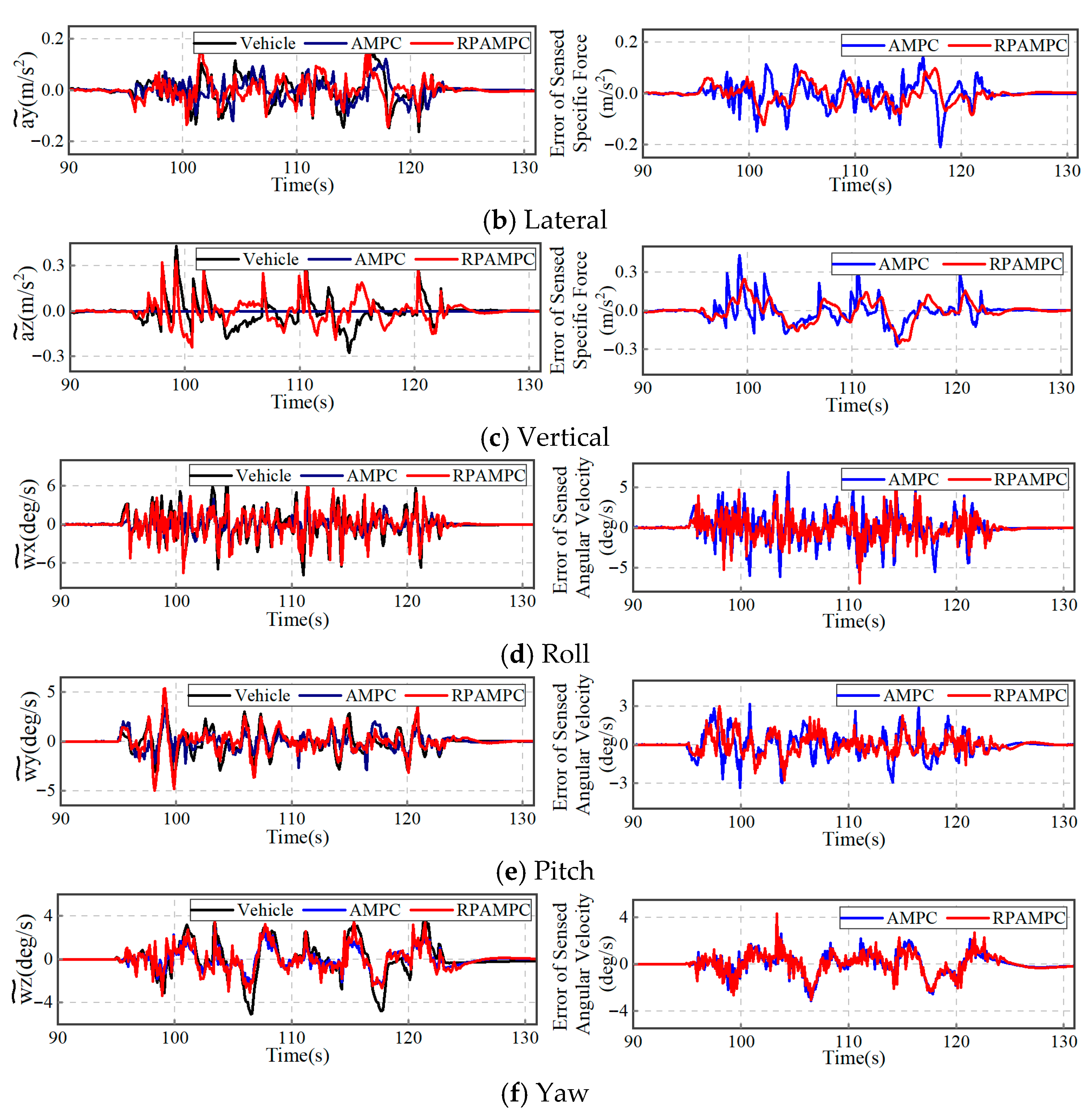
Given the motion range limitations of the simulation platform, the longitudinal, lateral, vertical, transverse, pitch, and yaw signals were scaled by factors of 0.1, 0.15, 0.1, 0.15, 0.15, and 0.15, respectively. This scaling was implemented to prevent excessive acceleration and angular velocity from causing the simulation platform to exceed its operational limits. Figure 9 presents the comparison results between AMPC-MCA, RPAMPC-MCA, and actual perception under road grade G. The results indicate that, compared to AMPC-MCA, RPAMPC-MCA significantly enhances motion cueing quality across all motion channels. Specifically, compared to AMPC-MCA, RPAMPC-MCA improves the correlation with actual perception by 25.11%, 19.99%, 35.82%, 26.43%, 23.51%, and 2.35% in the longitudinal, lateral, vertical, pitch, roll, and yaw channels, respectively. Additionally, in terms of RMSE, RPAMPC-MCA demonstrates lower errors. Compared to AMPC-MCA, RPAMPC-MCA reduces RMSE in the six channels by 25.21%, 18.39%, 7.9%, 19.63%, 23.95%, and 1.13%, respectively. These results clearly demonstrate that incorporating route preview into the AMPC framework significantly enhances the consistency between the motion cues and the actual vehicle motion, thereby effectively reducing the perceptual discrepancies between the real vestibular sensations and the simulated platform motion.
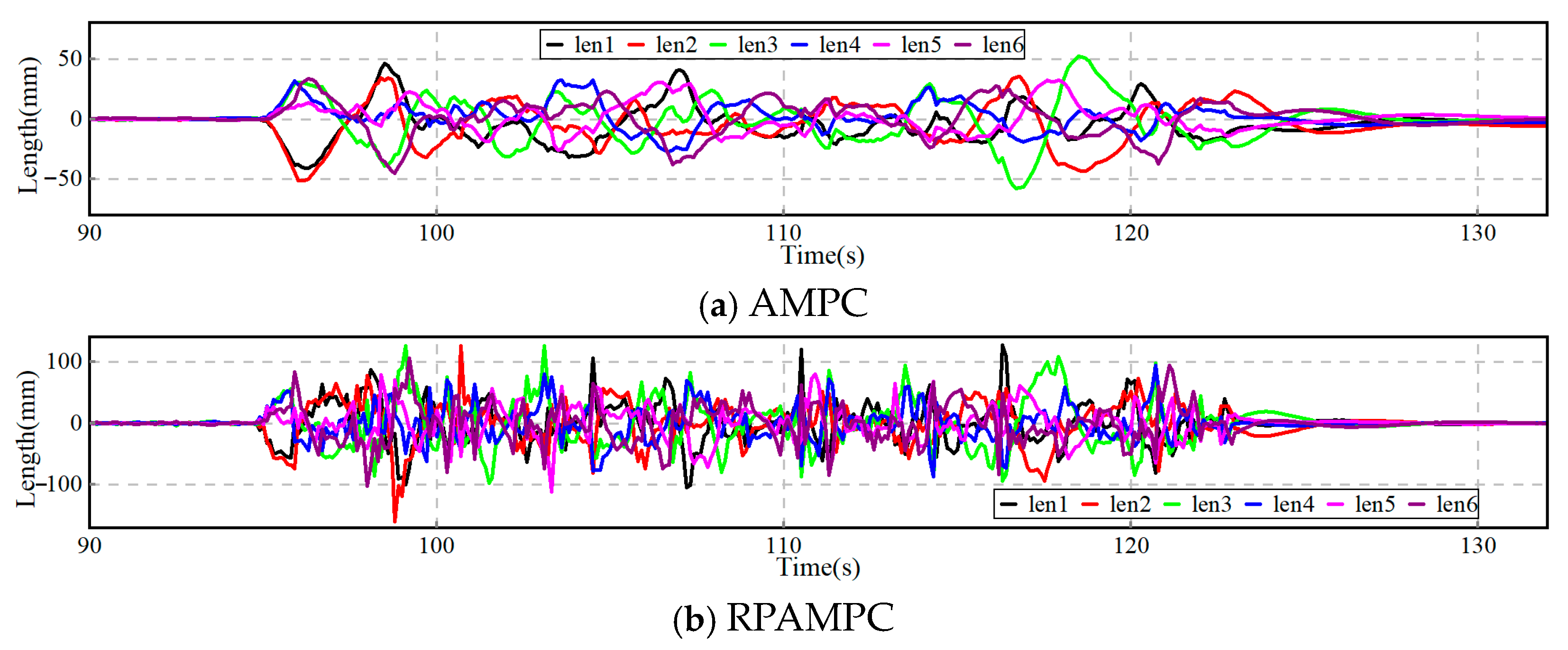
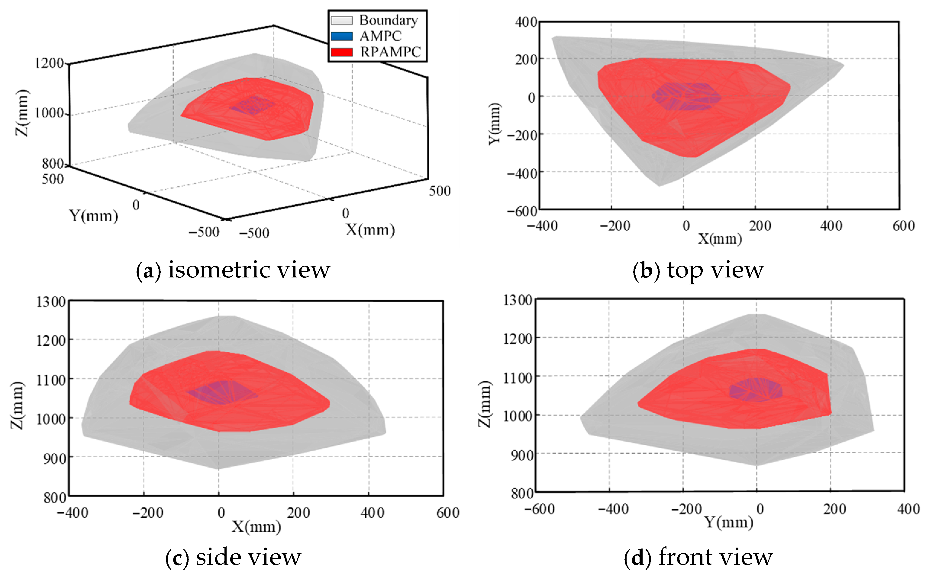
Figure 10 illustrates the actuator motion trajectories under AMPC and RPAMPC. Compared to AMPC, the actuator motion under RPAMPC shows greater amplitudes and more frequent variations. Furthermore, based on the actuator motions derived from the two control strategies, the workspace of the motion simulation platform has been calculated. As shown in Figure 11, the workspace corresponding to RPAMPC is larger than that corresponding to AMPC. Specifically, the workspace envelope area under AMPC is 0.0053 m3, whereas that under RPAMPC is 0.0222 m3, an increase of 318%. Thus, it can be inferred that RPAMPC-MCA utilizes the motion simulation platform’s workspace more efficiently.
Similarly, the motion cueing performance of AMPC-MCA and RPAMPC-MCA was evaluated under road grades C and E, with the results presented in Table 2. Under road grade C, compared to AMPC-MCA, the RPAMPC-MCA approach improved the correlation in the longitudinal, lateral, vertical, pitch, roll, and yaw channels by 8.38%, 4.37%, 24.96%, 11.1%, 10.4%, and 3.2%, respectively. Meanwhile, the RMSE values for these channels were reduced by 4.8%, 5.8%, 1.5%, 18.7%, 13.3%, and 1.12%, respectively. Under road grade E, compared to AMPC-MCA, RPAMPC-MCA improved the correlation in the longitudinal, lateral, vertical, pitch, roll, and yaw channels by 5.39%, 3.38%, 7.05%, 38.65%, 44.75%, and 6.3%, respectively. Correspondingly, the RMSE values decreased by 7.35%, 3.4%, 22.3%, 29.5%, 33.55%, and 7.11%, respectively.
Figure 12 illustrates the relative improvement in motion cueing quality of RPAMPC-MCA over AMPC-MCA under road grades C, E, and G. The results indicate that among the six channels, the vertical, pitch, and roll channels exhibit the most significant enhancements in motion cueing quality, suggesting that these channels are most affected by road conditions. Furthermore, closer observation reveals that the degree of improvement in the vertical, pitch, and roll channels is approximately proportional to the roughness of the road surface. For the longitudinal and lateral channels, the improvements are minimal under road grades C and D but become pronounced under grade E. This suggests that under road grades C and D, longitudinal and lateral motions are mainly governed by driver inputs, but as road roughness increases, road surface factors become the dominant influence. In contrast, the yaw channel exhibits negligible improvement across grades C, D, and E, suggesting its dependence on driver inputs rather than road surface characteristics.

5. Conclusions

To improve motion cueing precision in driving simulators operating under complex road conditions, this paper proposes an AMPC-based MCA with route preview. A dynamic prediction model for vehicle trajectories, driven by front-terrain data, is developed using deep learning techniques. Additionally, the state-space equations of the motion simulation platform are derived, incorporating actuator stroke and velocity states. An AMPC-based MCA is then formulated based on these models. In comparison to traditional AMPC-MCA, the proposed algorithm exhibits significant improvements across six motion channels (longitudinal, lateral, vertical, pitch, roll, and yaw) under road grade G. Specifically, the correlation scores increased by 25.11%, 19.99%, 35.82%, 26.43%, 23.51%, and 2.35%, respectively, while the RMSE decreased by 25.21%, 18.39%, 7.9%, 19.63%, 23.95%, and 1.13%, respectively, and workspace utilization rose by 318%. Furthermore, under road grades C and E, the proposed algorithm achieves consistent enhancements across all six degrees of freedom, with the vertical, pitch, and roll channels exhibiting the greatest improvements, followed by the longitudinal and lateral channels, while the yaw channel shows minimal improvement.
Despite these promising results, several limitations remain. Specifically, the experimental validation was conducted under a fixed and invariant set of road conditions, which may not fully capture the generalizability of the proposed algorithm. Future work may extend the framework to dynamically changing terrains, longer preview horizons, and alternative prediction models. In addition, integrating human-in-the-loop driving experiments and physiological measurements could enable a more comprehensive assessment of motion cueing performance.

Author Contributions

Conceptualization, X.J.; Methodology, X.J.; Software, B.Z. and X.C.; Validation, X.J. and B.Z.; Formal analysis, H.Z.; Investigation, X.J.; Resources, X.C.; Data curation, X.J.; Writing—original draft preparation, X.J.; Writing—review and editing, B.Z.; Visualization, H.Z.; Supervision, L.Z.; Project administration, L.Z.; Funding acquisition, L.Z. All authors have read and agreed to the published version of the manuscript.

Funding

This research was funded by National Natural Science Foundation grant number 51875499.

Data Availability Statement

The data that support the findings of this study are available from the corresponding author upon reasonable request.

Conflicts of Interest

On behalf of all the authors, the corresponding author states that there is no conflict of interest.

References

  1. Olivari, M.; Pretto, P.; Venrooij, J.; Bülthoff, H. Defining the kinematic requirements for a theoretical driving simulator. Transp. Res. Part F Traffic Psychol. Behav. 2019, 61, 5–15. [Google Scholar] [CrossRef]
  2. Jiang, X.; Chen, X.; Jiao, Y.; Zhang, L. Objective Evaluation of Motion Cueing Algorithms for Vehicle Driving Simulator Based on Criteria Importance through Intercriteria Correlation (CRITIC) Weight Method Combined with Gray Correlation Analysis. Machines 2024, 12, 344. [Google Scholar] [CrossRef]
  3. Kim, J.; Lee, S.-M.; Son, H.; Park, T. Effects of unlimited angular motion cue and cue discrepancy on simulator sickness. Expert Syst. Appl. 2023, 213, 119196. [Google Scholar] [CrossRef]
  4. Meyer, M.-A.; Sauter, L.; Granrath, C.; Hadj-Amor, H.; Andert, J. Simulator Coupled with Distributed Co-Simulation Protocol for Automated Driving Tests. Automot. Innov. 2021, 4, 373–389. [Google Scholar] [CrossRef]
  5. Cleij, D.; Venrooij, J.; Pretto, P.; Katliar, M.; Bülthoff, H.H.; Steffen, D.; Hoffmeyer, F.W.; Schöner, H.-P. Comparison between filter-and optimization-based motion cueing algorithms for driving simulation. Transp. Res. Part F Traffic Psychol. Behav. 2019, 61, 53–68. [Google Scholar] [CrossRef]
  6. Berthoz, A.; Bles, W.; Bülthoff, H.H.; Grácio, B.C.; Feenstra, P.; Filliard, N.; Huhne, R.; Kemeny, A.; Mayrhofer, M.; Mulder, M.; et al. Motion scaling for high-performance driving simulators. IEEE Trans. Hum.-Mach. Syst. 2013, 43, 265–276. [Google Scholar] [CrossRef]
  7. Ellensohn, F.; Venrooij, J.; Schwienbacher, M.; Rixen, D. Experimental evaluation of an optimization-based motion cueing algorithm. Transp. Res. Part F Traffic Psychol. Behav. 2019, 62, 115–125. [Google Scholar] [CrossRef]
  8. Jain, V.; Kumar, S.S.; Papaioannou, G.; Happee, R.; Shyrokau, B. Optimal trajectory planning for mitigated motion sickness: Simulator study assessment. IEEE Trans. Intell. Transp. Syst. 2023, 24, 10653–10664. [Google Scholar] [CrossRef]
  9. Bruschetta, M.; Cenedese, C.; Beghi, A. A real-time, MPC-based motion cueing algorithm with look-ahead and driver characterization. Transp. Res. Part F Traffic Psychol. Behav. 2019, 61, 38–52. [Google Scholar] [CrossRef]
  10. Conrad, B.; Schmidt, S.F. A Study of Techniques for Calculating Motion Drive Signals for Flight Simulators; No. NASA-CR-114345; NASA Technical Reports Server: Hampton, VA, USA, 1971.
  11. Parrish, R.V.; Dieudonne, J.E.; Bowles, R.L.; Martin, D.J., Jr. Coordinated adaptive washout for motion simulators. J. Aircr. 1975, 12, 44–50. [Google Scholar] [CrossRef]
  12. Asadi, H.; Mohamed, S.; Nahavandi, S. Incorporating human perception with the motion washout filter using fuzzy logic control. IEEE/ASME Trans. Mechatron. 2015, 20, 3276–3284. [Google Scholar] [CrossRef]
  13. Zhiyong, T.; Hu, M.; Zhongcai, P.; Jinhui, Z. Adaptive motion cueing algorithm based on fuzzy tuning for improving human sensation. In Proceedings of the 2016 IEEE Chinese Guidance, Navigation and Control Conference (CGNCC), Nanjing, China, 12–14 August 2016; pp. 1200–1205. [Google Scholar]
  14. Garrett, N.J.; Best, M.C. Evaluation of a new body-sideslip-based driving simulator motion cueing algorithm. Proc. Inst. Mech. Eng. Part D J. Automob. Eng. 2012, 226, 1433–1444. [Google Scholar] [CrossRef]
  15. Pais, A.V.; Wentink, M.; van Paassen, M.M.; Mulder, M. Comparison of three motion cueing algorithms for curve driving in an urban environment. Presence 2009, 18, 200–221. [Google Scholar] [CrossRef]
  16. Qazani, M.R.C.; Asadi, H.; Khoo, S.; Nahavandi, S. A linear time-varying model predictive control-based motion cueing algorithm for hexapod simulation-based motion platform. IEEE Trans. Syst. Man Cybern. Syst. 2019, 51, 6096–6110. [Google Scholar] [CrossRef]
  17. Qazani, M.R.C.; Asadi, H.; Mohamed, S.; Lim, C.P.; Nahavandi, S. A time-varying weight MPC-based motion cueing algorithm for motion simulation platform. IEEE Trans. Intell. Transp. Syst. 2021, 23, 11767–11778. [Google Scholar] [CrossRef]
  18. Asadi, H.; Bellmann, T.; Qazani, M.C.; Mohamed, S.; Lim, C.P.; Nahavandi, S. A novel decoupled model predictive control-based motion cueing algorithm for driving simulators. IEEE Trans. Veh. Technol. 2023, 72, 7024–7034. [Google Scholar] [CrossRef]
  19. Biemelt, P.; Link, C.; Gausemeier, S.; Trächtler, A. A model-based online reference prediction strategy for model predictive motion cueing algorithms. IFAC-PapersOnLine 2020, 53, 6082–6088. [Google Scholar] [CrossRef]
  20. Lamprecht, A.; Steffen, D.; Nagel, K.; Haecker, J.; Graichen, K. Online model predictive motion cueing with real-time driver prediction. IEEE Trans. Intell. Transp. Syst. 2021, 23, 12414–12428. [Google Scholar] [CrossRef]
  21. ISO 8608:2016; Mechanical Vibration—Road Surface Profiles—Reporting of Measured Data. International Organization for Standardization: Geneva, Switzerland, 2016.
  22. Harrison, M.F. Low-Frequency Vibrations in Disk Braking Systems—Controlling the Creep-Groan Phenomenon in Road Vehicles; Professional Engineering Publishing Ltd.: Westminister, UK, 2004. [Google Scholar]
  23. Grigoriu, M. On the spectral representation method in simulation. Probabilistic Eng. Mech. 1993, 8, 75–90. [Google Scholar] [CrossRef]
  24. Min, H.; Xiong, X.; Wang, P.; Zhang, Z. A Hierarchical LSTM-Based Vehicle Trajectory Prediction Method Considering Interaction Information. Automot. Innov. 2024, 7, 71–81. [Google Scholar] [CrossRef]
  25. Yang, N.; Song, Z.; Amini, M.R.; Hofmann, H. Internal Short Circuit Detection for Parallel-Connected Battery Cells Using Convolutional Neural Network. Automot. Innov. 2022, 5, 107–120. [Google Scholar] [CrossRef]
  26. Ormsby, C.C. Model of Human Dynamic Orientation. Ph.D. Thesis, Massachusetts Institute of Technology, Cambridge, MA, USA, 1974. [Google Scholar]
  27. Qazani, M.R.C.; Asadi, H.; Bellmann, T.; Mohamed, S.; Lim, C.P.; Nahavandi, S. Adaptive washout filter based on fuzzy logic for a motion simulation platform with consideration of joints’ limitations. IEEE Trans. Veh. Technol. 2020, 69, 12547–12558. [Google Scholar] [CrossRef]
  28. Xu, G.; Chen, M.; He, X.; Liu, Y.; Wu, J.; Diao, P. Research on state-parameter estimation of unmanned Tractor—A hybrid method of DEKF and ARBFNN. Eng. Appl. Artif. Intell. 2024, 127, 107402. [Google Scholar] [CrossRef]
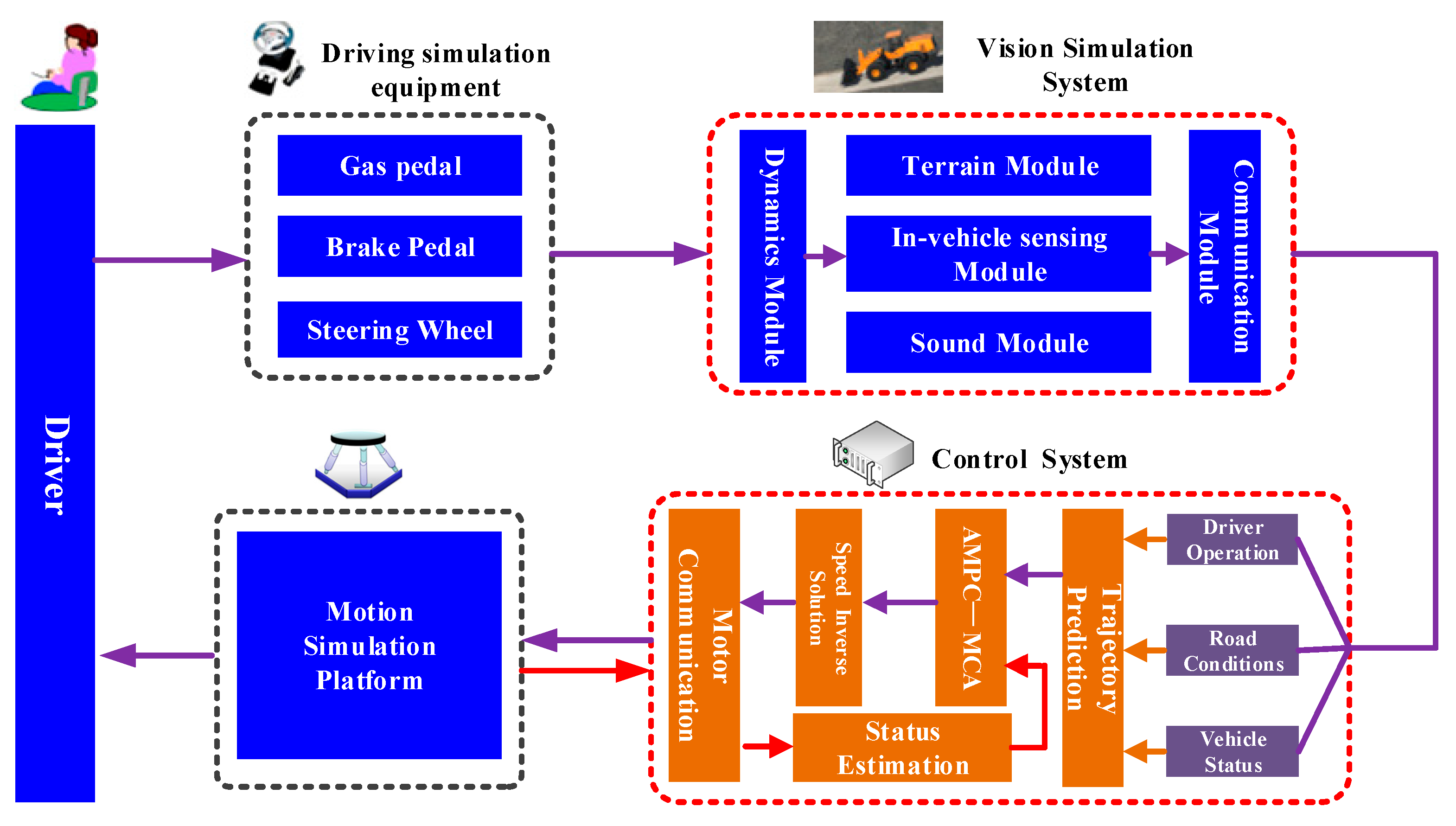
Figure 1. Overall control framework of the route-preview AMPC-based MCA for the driving simulator. The trajectory module predicts the vehicle’s future accelerations and angular velocities by exploiting forward terrain information together with the vehicle’s states and driver inputs. The AMPC-MCA module subsequently computes the optimal platform control inputs based on the current platform states and the predicted future vehicle motion.
Actuators 14 00588 g001
Figure 2. Vehicle sensor layout and measurement.
Actuators 14 00588 g002
Figure 3. Different grade elevation maps and their corresponding road scenes.
Actuators 14 00588 g003
Figure 4. The network structure for vehicle trajectory prediction.
Actuators 14 00588 g004
Figure 5. Prediction accuracy under different lengths of time series.
Actuators 14 00588 g005
Figure 6. Motion simulation platform structure sketch.
Actuators 14 00588 g006
Figure 7. Adaptive model predictive control block diagram.
Actuators 14 00588 g007
Figure 8. Driving simulator-related physical objects and driving scenes.
Actuators 14 00588 g008
Figure 9. Comparison of motion cueing based on AMPC and RPAMPC with actual vehicle motion perception and its perception error.
Actuators 14 00588 g009aActuators 14 00588 g009b
Figure 10. Motion travel of the actuators based on AMPC and RPAMPC.
Actuators 14 00588 g010
Figure 11. Position of the workspace based on AMPC and RPAMPC.
Actuators 14 00588 g011
Figure 12. Comparison of the relative improvement in motion cueing quality achieved by RPAMPC-MCA compared to AMPC-MCA for road grades C, E, and G.
Actuators 14 00588 g012
Table 1. Road roughness coefficient.
IndexABCDEFGH
G d ( n 0 ) 16642561024409616,38465,536262,144
G d ( n 0 ) : Road roughness coefficient, with units of 10−6 m2/m−1 and n 0 = 0.1 m−1.
Table 2. Objective evaluation based on AMPC and RPAMPC.
CCRMSE
AMPCRPAMPCAMPCRPAMPC
a x ˜ C0.48880.57260.06570.0625
E0.6410.69490.05440.0504
G0.49280.75390.02300.0172
a y ˜ C0.31060.35430.03420.0322
E0.57390.60770.050.0483
G0.49590.69580.02230.0182
a z ˜ C0.20610.45570.0460.0453
E0.60770.67820.03810.0296
G0.17770.53590.0430.0396
w x ˜ C0.49720.60821.27521.0362
E0.36080.74731.57051.1072
G0.47110.73540.87060.6997
w y ˜ C0.18210.28610.76940.6670
E0.23770.68520.99680.6623
G0.57410.80920.45340.3448
w z ˜ C0.63590.63910.73560.7219
E0.87230.87862.02701.8828
G0.82490.80140.44360.4386
Disclaimer/Publisher’s Note: The statements, opinions and data contained in all publications are solely those of the individual author(s) and contributor(s) and not of MDPI and/or the editor(s). MDPI and/or the editor(s) disclaim responsibility for any injury to people or property resulting from any ideas, methods, instructions or products referred to in the content.