Abstract
A fault-tolerant controller design for reusable launch vehicles (RLVs) is discussed in this paper. The control precision of RLVs is very important, since it must be ensured that an RLV’s speed reaches zero while flying to the target point. More seriously, the rocket’s thrust system may suffer from faults, so the fault-tolerant control of RLVs is very important. The landing dynamic model of RLVs is very complex, and the thrust is coupled with time-varying states, which make the controller design of RLVs very difficult. Based on the specific control requirements of rocket landing, the control design problem is first transformed into a normal model in this paper. Then, considering potential thrust faults, an optimal fault-tolerant controller is designed using reinforcement learning. Considering sensor faults and actuator faults, this paper presents the corresponding fault-tolerant controller design method. Considering that the analytical problem of the proposed fault-tolerant controller is difficult to solve, this paper presents an approximation method for the analytical solution based on a neural network. The simulation results demonstrate that the proposed controller ensures the safe and stable landing of the rocket in both nominal and fault scenarios.
1. Introduction
With the global development of outer space, RLVs have become a prominent focus of research [1]. RLVs have significant advantages, including rapid deployment, large load carrying capacity, and reusability, and all of these advantages substantially reduce the cost of space transportation and exploration. However, to enable reuse ability, RLVs must perform vertical landings with high precision, placing stringent demands on their guidance and control systems [2,3].
In the vertical recovery of RLVs, the control force is provided by the rocket’s thrust. During the landing process, the control objective of RLVs is to ensure that they reach the target landing point smoothly while minimizing fuel consumption. In this phase, the only adjustable control input is the magnitude and direction of the thrust. However, the system must simultaneously control the rocket’s position to the target and reduce its velocity to zero, which means that there are six outputs to be controlled and three control inputs. This mismatch between the number of control inputs (thrust magnitude and direction) and controlled outputs (position and velocity states) makes the rocket landing problem a typical underactuated control problem. However, to ensure a smooth landing, both the position and velocity of the rocket must be simultaneously regulated. The recovery of launch vehicles represents a typical underactuated control problem.
The design of the optimal controller for an underactuated system is challenging [4,5]. To achieve this, a trajectory tracking control law based on the dynamic inversion method combined with an online trajectory update strategy is proposed in [6]; by using this method, effective reentry guidance tracking is achieved. Sliding mode dynamic surface control is employed to design a precise vertical recovery control strategy, ensuring high control accuracy during vertical recovery [7]. A two-point boundary value approach, formulating the rocket’s initial and desired states as boundary conditions to optimize the trajectory, is introduced in [8,9]; subsequently, an indirect method was used to design the rocket’s optimal flight path. However, the indirect method faces challenges in real-time implementation and convergence guarantees. A direct method for designing controllers for rocket recovery by solving convex optimization problems to achieve landing control is proposed in [10,11]. Nevertheless, both direct and indirect methods require accurate knowledge of the rocket’s nonlinear model and disturbances. In practice, due to the complex atmospheric environment and machining accuracy limitations, the RLV model inevitably contains uncertainties. Moreover, the rocket operates over a large envelope, and states of RLVs are coupled with each other, which leads to the complexity of the controller design of RLVs [12,13].
For the rocket landing control problem under uncertainties and model deviations, the indirect method is improved by neural networks [14,15]. A large set of rocket landing sample data is obtained by extensive training, and then neural networks are used to fit the data; thus a new empirical control law that achieves rocket landing control is derived. By applying reinforcement learning, a staged reward function is built [16]. The staged reward function is solved by Q-learning, and then a rocket landing controller is optimized under energy constraints. Ref. [17] analyzes the uncertain factors of RLVs and presents a design method for parameterized controllers.
The rocket landing control problem has attracted widespread attention. Researchers have designed landing controllers using methods such as direct approaches, indirect approaches, neural networks, and reinforcement learning. However, in practical applications, rocket thrust systems may experience faults, which significantly complicate landing control under fault conditions. The attitude FTC problem for faulty rocket systems is proposed, and a robust control method based on fixed-time observers is proposed [18]. An adaptive FTC technique for rocket attitude control systems is presented in [19]. The FTC problem of the attitude control system during rocket reentry is discussed in [20]. Nevertheless, fault-tolerant control in the rocket landing and recovery process remains relatively underexplored and lacks a comprehensive solution. In summary, although the rocket landing problem has received considerable attention, existing studies have yet to address fault-tolerant control in rocket landing guidance.
Based on the above discussion, this paper discusses the fault-tolerant landing controller designing of RLVs. Uncertainties such as inaccurate nonlinear rocket models and unknown external disturbances are taken into account. While considering these uncertainties and disturbances, neural networks are employed to construct the performance function and control law within the rocket controller, and a model-free fault-tolerant control design method is proposed. The contributions of this paper can be summarized as follows:
- A data-based FTC method for RLVs is proposed in this paper. The proposed method can realize the accurate control of RLVs without complete information on the RLV’s nonlinear model.
- Both the uncertainties and external interference of RLVs are considered in this paper. The proposed method can deal with not only the faults of RLVs but also their uncertainties and external interference.
- Both sensor faults and partial failure faults are considered and addressed simultaneously within the proposed FTC method.
2. Landing Model of Reusable Launch Vehicle
2.1. Nonlinear Landing Model of Reusable Launch Vehicle
The rocket landing problem can be described by the following nonlinear dynamic equations:
where represents the position vector of the rocket; represents the velocity vector; denotes the mass of the rocket; represents the consumption rate of mass, that is, the consumption rate of fuel; and is the gravitational acceleration at the rocket’s location. denotes the thrust vector of the rocket, and represents the rocket’s exhaust velocity, which is a constant. stands for the aerodynamic drag experienced by the rocket, which depends on the vehicle’s velocity and is calculated simultaneously using the following equation:
where is the atmospheric density, which depends on the rocket’s position; is the aerodynamic reference area of the rocket; is the drag coefficient, which is related to the rocket’s Mach number.
To ensure control accuracy, is closely related to the rocket’s altitude. In practical applications, is calculated using the following formula:
where is the Earth’s gravitational constant, and is the vector from the Earth’s center to the surface.
2.2. Control Requirements
The control objective can be formulated as the following optimal control problem:
where denotes the initial time, and represents the final landing time. correspond to the position, velocity, and mass at the initial time, respectively. denotes the exhaust velocity. The rocket’s intrinsic constraints are taken into account; specifically, the thrust is bounded as , where are positive real numbers.
3. Model Transformation
By examining Equations (1)–(3) and considering the control requirements, the variables to be controlled include the position and velocity in three directions, as well as the rocket’s mass. However, the available control input is limited to the rocket’s thrust, so this problem is a typical underactuated control problem. To facilitate controller design, the model is transformed according to the control requirements.
3.1. Selection of Control Variables
To facilitate the controller design, the RLV’s position and velocity are decomposed in the North–East–Up coordinate frame. In this coordinate system, both the position and velocity of the rocket are represented as three-dimensional state variables. Meanwhile, the thrust of the rocket is also decomposed accordingly. Assuming that the rocket does not rotate in space, the thrust can be expressed as a three-dimensional control input vector.
where denotes the angle between the thrust vector and the east direction in the “north-east” plane, while represents the angle between the thrust vector and the “upward” (zenith) axis. Under this configuration, the constraints on the three input variables of the rocket are given as follows:
3.2. Fully Actuated System
To facilitate controller design, the rocket landing model is transformed based on control requirements. Let and , where denotes the position vector of the rocket expressed in the local East–North–Up coordinate system, and represents the velocity vector in the same coordinate frame. The nonlinear dynamics of the rocket can then be rewritten as follows:
where
At this stage, the rocket landing problem is transformed into a control problem with three inputs and three outputs, where the control objectives achieve and while maximizing the remaining fuel.
To address the above control problem, new output variables are selected as follows:
where represents the coupling between position and velocity. The value of r is a positive number, and the specific value is determined by the importance of position control accuracy and speed control accuracy. Then the new equation can be expressed as follows:
The specific form of is determined by Equations (1), (2) and (5).
4. Fault Description of RLVs
The RLV’s thrust is controlled by an onboard computer. The thrust system itself may exhibit deviations. In particular, the erosion of the thrust system’s nozzle may occur, causing the rocket’s thrust vector to deviate from the desired direction; then the control accuracy of the rocket is affected. In this paper, two common fault modes are considered for the design of a fault-tolerant controller for the rocket.
4.1. Partial Failure Fault
The rocket propulsion system may produce a thrust lower than the expected value. This type of fault can be described as follows:
where denotes the desired thrust of the rocket, i.e., the thrust required under fault-free conditions; represents the actual thrust that the rocket can provide; and indicates the thrust efficiency of the rocket, with . In this scenario, the rocket experiences a partial failure fault. Considering the actual occurrence of faults in the rocket, the efficiency is unknown. Under this fault mode, the rocket control problem can be transformed into the following:
4.2. Sensor Fault
The rocket’s thrust command is generated by converting the electrical signals received from the onboard computer. However, during signal transmission, signal attenuation may occur, causing the electrical signal received by the thrust generation system to be lower than the expected value. As a result, the rocket’s thrust will deviate. The thrust can be expressed as follows:
where denotes the desired thrust of the rocket, and represents the thrust error caused by the sensor fault. is a time-varying variable. This type of fault is defined as a sensor fault, with a critical threshold for thrust loss caused by the fault given by . represents the actual thrust of the rocket. Under this fault mode, the rocket’s control problem can be formulated as follows:
5. Design of Optimal Fault-Tolerant Controller
By analysis, the aforementioned FTC problem is a nonlinear time-varying control problem. Moreover, the inputs are not given in an explicit form, and there is coupling among the input variables; all of this makes the direct FTC design of RLVs challenging. To achieve optimal control for (9) and (11), a model-free optimal fault-tolerant controller is considered, and a data-driven online solution method based on reinforcement learning is employed to implement the optimal controller.
5.1. Optimal Fault-Tolerant Controller Design for Partial Actuator Failures
5.1.1. Optimal Fault-Tolerant Controller Design
Considering the partial failure model of the rocket described in Equation (8), the controllable inputs available from the rocket can be represented as follows:
Since and are unknown, the exact form of cannot be determined. Considering that the optimization objective of rocket landing is to minimize fuel consumption while ensuring a stable landing, the following performance index is selected as the optimization criterion:
where and are positive definite weighting matrices
Remark 1.
Regarding the optimization criterion (9), the control objective is to ensure that the rocket reaches the designated landing point while minimizing fuel consumption. In performance index (12), by appropriately selecting the weighting matrices and , the optimization criterion (9) can be effectively optimized. Therefore, the performance index (12) is reasonable.
For the control system (9), combined with the performance index function established in (12), the following Hamilton–Jacobi–Bellman (HJB) function is defined:
where is the gradient of the performance index . According to optimal control theory, the required optimal controller can guarantee the minimization of the following performance index:
Under the action of this controller,
To solve the above HJB equation, the partial derivatives should equal zero:
The optimal control input which can ensure that the performance index (12) reaches the minimum under given constraints can be obtained
Substituting the optimal control input into Equation (13) yields
By substituting the optimal control input into Equation (13), the optimal control law (14) is obtained, which serves as the optimal controller for the system under partial actuator failures. However, this optimal controller cannot be directly implemented since the gradient of the performance index function (12), denoted as , cannot be solved analytically. To better solve the optimal control input, a policy iteration method from reinforcement learning is employed to compute the system’s optimal control.
The online solution of the optimal controller can be achieved through Algorithm 1.
| Algorithm 1: Policy iterative algorithm of FTC |
| Initialization: Select |
| Step1: pass |
| Calculate |
| Step2: Updated Control Input |
| If , then stop the computation; otherwise, proceed to Step 1. Here, is a sufficiently small positive constant. |
5.1.2. Online Solution Method for Fault-Tolerant Controller
For the nonlinear model (9) proposed in this paper, directly applying Algorithm 1 to iteratively compute the controller solution is highly challenging, since the model parameters are time-varying and the fault variable is unknown. Under such circumstances, this paper proposes an online iterative solution method. Considering the performance index (12) and the controller (14), the following neural network is selected for online approximation:
where denotes the weight matrix of the performance evaluation neural network, and represents its basis function; is the weight matrix of the controller neural network, and denotes its basis function. The terms and represent the approximation errors.
Assuming that both the weights and basis functions in (15) are bounded, the rocket dynamics described in (12) can be rewritten under the conditions of the controller (14). The following can be obtained:
The update law for the optimal control is given by the following:
The HJB equation is as follows:
where and represent the optimal weights of the chosen performance approximation neural network and the controller neural network, respectively. Since the optimal weights are unknown, let and denote the estimates of these optimal weights. Therefore,
Then the HJB equation is
where denotes the estimated total error.
The residual error of the system at this moment is
To better represent the residual error and facilitate subsequent derivations, a new weight vector is defined as follows:
The residual error can be expressed as
where
To address the above issues, the following weight update law is designed:
where denotes the adjustable learning rate.
Theorem 1.
For the RLV landing system (9) subject to partial actuator failures, to achieve the optimal performance index (12), the controller defined by Equation (15) is employed, and the update law for the controller and performance approximation network follows Equation (20). Under these conditions, the landing system remains stable and reaches the desired landing point.
Proof.
Choose the Lyapunov function as follows:
where ; taking the derivative of the above equation yields the following:
Based on Equation (12),
where . Substituting this into the Hamiltonian function yields
Based on the neural network weight formulation,
For Equation (18),
Let and , where ; therefore , and and are bounded normal variables.
For
Therefore, . According to the theory of bounded stability of the system [20], the system is boundedly stable. The proof is completed. □
Remark 2.
In the design of partially faulty controllers, thrust efficiency is unknown. However, during system derivation, neural network approximation treats the input matrix and efficiency as a combined entity, thereby simultaneously addressing the uncertainties in both the input matrix and efficiency.
5.2. Design of Fault-Tolerant Controller for Sensor Failures
In Section 5.1, the optimal controller for the landing rocket under partial failure conditions was obtained. This section analyzes the fault-tolerant control problem of the rocket under sensor failure conditions.
The model of the rocket considering sensor failures, as established in Section 3.2, can represent the overall landing rocket system under this fault mode as follows:
where represents the thrust loss of the rocket caused by the fault. At this point, according to the performance function in Section 5.1, its derivative is taken.
Based on the HJB equation, a further simplification of the above expression yields the following:
It can be seen that the designed fault-tolerant controller needs to compensate for the efficiency loss of the actuators caused by faults. Under the premise that the optimal controller for the nominal condition is known, the fault-tolerant controller for rocket landing is implemented as follows:
Theorem 2.
For the RLV landing system described by (9), to satisfy the optimal performance criterion in (12), a controller as given in (22) is employed. The update laws for both the controller and the performance approximation network follow (20), while the adaptive estimation parameter update law for faults is given by (23). Under these conditions, the landing system remains stable and successfully reaches the desired landing point.
where denotes the maximum value of the function.
Proof.
Choose the Lyapunov function as follows:
where , and is a constant. Taking the derivative of the above equation yields the following:
Based on Equation (12), considering ,
Then, combined with the proof of Theorem 1,
By combining this with the update law of , the system is shown to be bounded and stable, thus completing the proof. □
6. Simulation Results
To verify the performance of the proposed method, it is applied to the landing control of a recoverable rocket. In the simulation, the rocket’s initial position is set to , and the initial velocity is . The mass of the rocket is 48,200 kg, and the rocket’s fault conditions are configured as follows:
(1) For partial failure faults, ;
(2) For the sensor fault, N.
The basis function selected in the controller design is . According to the controller designed in this paper, simulations were first conducted under fault-free conditions. The proposed FTC is marked as , while a normal controller without considering the fault is marked as . The following three cases are considered in the simulation:
Case I: Only the partial failure fault is considered;
Case II: Only the sensor fault is considered;
Case III: Both the partial failure fault and the sensor fault are considered.
The simulation results for the above three cases are shown in the following figures.
Case I: Figure 1 represents the position variation curve, Figure 2 represents the velocity variation curve, Figure 3 shows the rocket’s thrust variation curve, and Figure 4 depicts the rocket’s mass variation curve. As shown in the figures, the designed FTC achieves the stable control of the rocket under fault-free conditions and ensures a stable landing.
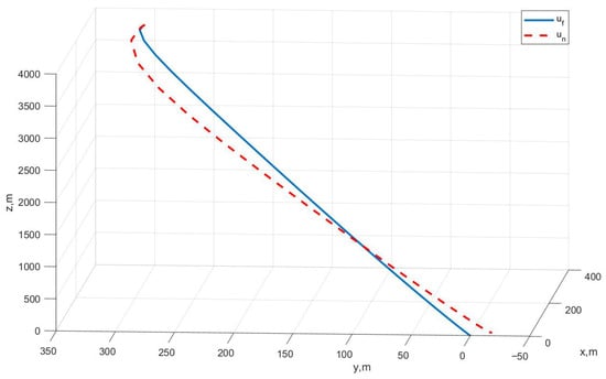
Figure 1.
Variation in rocket position under Case I.
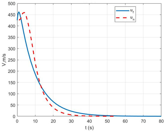
Figure 2.
Variation in rocket velocity under Case I.
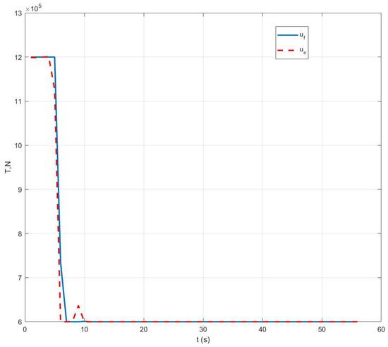
Figure 3.
Variation in rocket thrust under Case I.
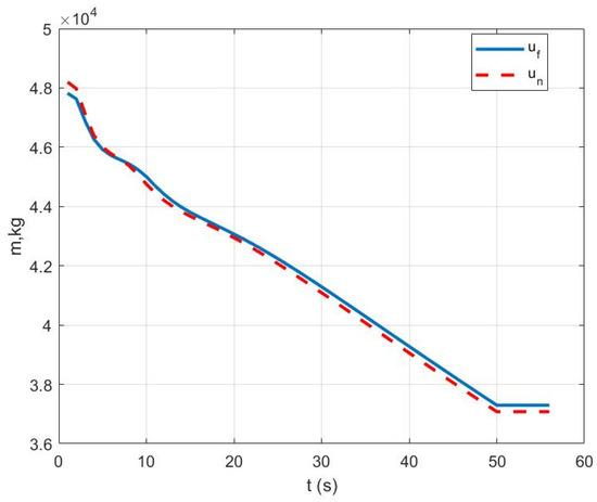
Figure 4.
Variation in rocket mass under Case I.
Case II: Figure 5 represents the position variation curve, Figure 6 represents the velocity variation curve, Figure 7 shows the rocket’s thrust variation curve, and Figure 8 depicts the rocket’s mass variation curve. As shown in the figures, under sensor fault, the designed FTC achieves the stable control of the rocket under fault-free conditions and ensures a stable landing.
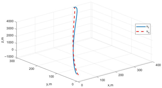
Figure 5.
Variation in rocket position under Case II.
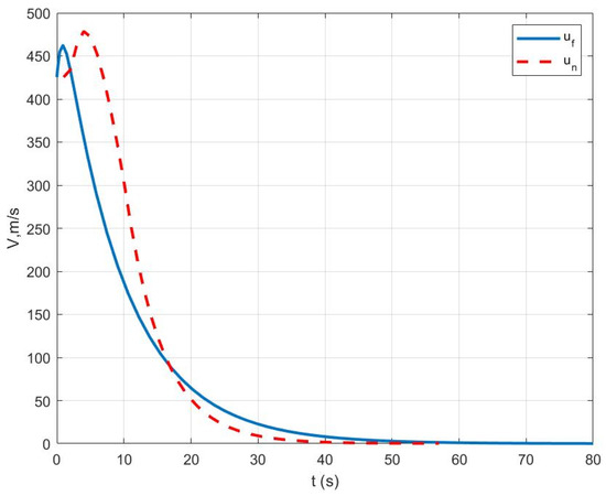
Figure 6.
Variation in rocket velocity under Case II.
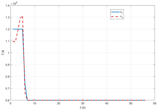
Figure 7.
Variation in rocket thrust under Case II.
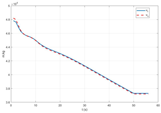
Figure 8.
Variation in rocket mass under Case II.
Case III: Figure 9 represents the position variation curve, Figure 10 represents the velocity variation curve, Figure 11 shows the rocket’s thrust variation curve, and Figure 12 depicts the rocket’s mass variation curve. As shown in the figures, the designed FTC achieves the stable control of the rocket under fault-free conditions and ensures a stable landing under both the partial failure fault and the sensor fault.
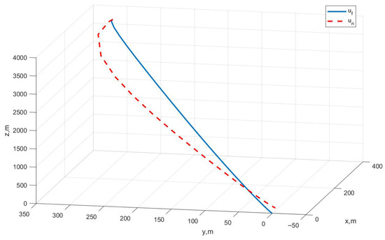
Figure 9.
Variation in rocket position under Case III.
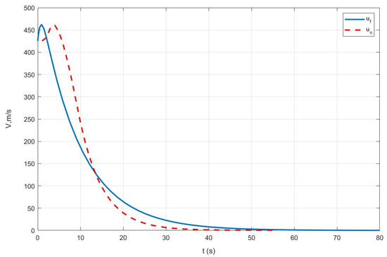
Figure 10.
Variation in rocket velocity under Case III.
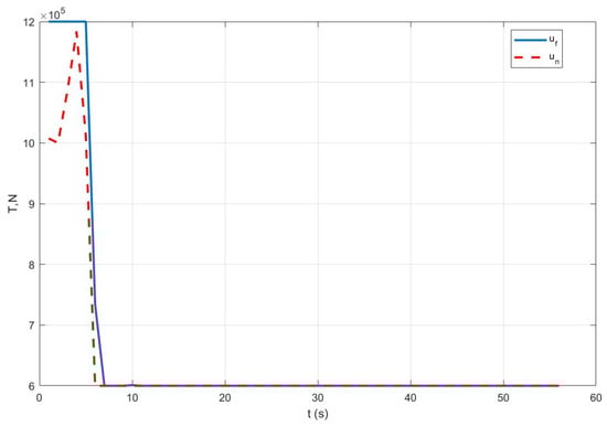
Figure 11.
Variation in rocket thrust under Case III.
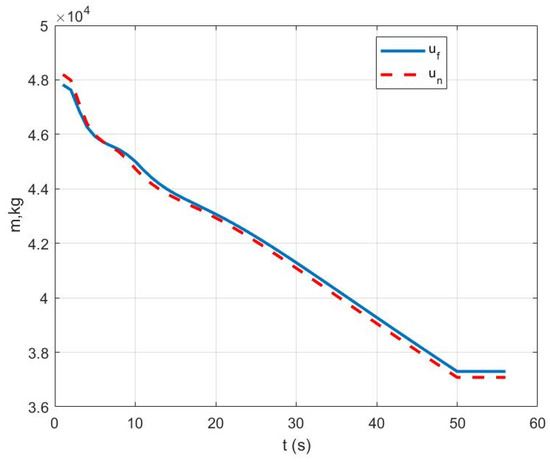
Figure 12.
Variation in rocket mass under Case III.
Based on the simulation results, it can be observed that when the system operates without faults, the designed controller is capable of achieving the safe landing control of the reusable launch vehicle. Furthermore, when faults occur, the designed controller can still ensure the safe landing control of the launch vehicle under fault conditions.
7. Conclusions
This paper addresses the landing problem of RLVs. By analyzing the landing rocket model, the typical underactuated control challenge of the rocket’s control system is identified. Subsequently, through model transformation, a controllable rocket landing model is derived. Considering the presence of uncertainties and external disturbances in the rocket model, a reinforcement learning-based controller is designed. Additionally, a fault-tolerant controller is developed to handle sensor faults in the rocket. The simulation results demonstrate that the proposed controllers ensure the safe and precise landing of the reusable launch vehicle under both fault-free and faulty conditions.
Author Contributions
Conceptualization, J.X. and X.H.; methodology, X.H.; software, Y.X.; validation, Y.W. and J.X.; investigation, X.H.; resources, Y.W.; data curation, C.G. and Y.X.; writing—original draft preparation, J.X.; writing—review and editing, C.G.; visualization, X.H.; supervision, X.H.; project administration, J.X.; funding acquisition, X.H. All authors have read and agreed to the published version of the manuscript.
Funding
This research was funded by the National Natural Science Foundation of China under Grant 61833016, Grant 62073265.
Institutional Review Board Statement
Not applicable.
Data Availability Statement
No new data were created or analyzed in this study.
Acknowledgments
We would like to acknowledge the reviewers for their careful reading, helpful comments, and constructive suggestions, which have significantly improved the presentation of our manuscript.
Conflicts of Interest
The authors declare no conflicts of interest.
References
- Hu, X.; Xiao, B.; Hu, C.; Si, X. Unmeasurable flexible dynamics monitoring and tracking controller design for guidance and control system of hypersonic flight vehicle. J. Frankl. Inst. 2024, 361, 958–977. [Google Scholar] [CrossRef]
- Wu, X.; Xiao, B.; Wu, C.; Guo, Y. Centroidal voronoi tessellation and model predictive control–based macro-micro trajectory optimization of microsatellite swarm. Space Sci. Technol. 2022, 2022, 9802195. [Google Scholar] [CrossRef]
- Gulczynski, M.T.; Vennitti, A.; Scarlatella, G.; Calabuig, G.J.D.; Blondel-Canepari, L.; Weber, F.; Sarritzu, A.; Bach, C.; Deeken, J.C.; Pasini, A.; et al. RLV applications: Challenges and benefits of novel technologies for sustainable main stages. In Proceedings of the International Astronautical Congress, IAC (No. 64293), Dubai, United Arab Emirates, 25–29 October 2021; International Astronautical Federation, IAF: Paris, France, 2021. [Google Scholar]
- Ye, L.; Tian, B.; Liu, H.; Zong, Q.; Liang, B.; Yuan, B. Anti-windup robust backstepping control for an underactuated reusable launch vehicle. IEEE Trans. Syst. Man Cybern. Syst. 2020, 52, 1492–1502. [Google Scholar] [CrossRef]
- Singh, S.; Stappert, S.; Buckingham, S.; Lopes, S.; Kucukosman, Y.C.; Simioana, M.; Pripasu, M.; Wiegand, A.; Sippel, M.; Planquart, P. Dynamic Modelling and control of an aerodynamically controlled capturing device for ‘in-air-capturing’ of a reusable launch vehicle. In Proceedings of the 11th International ESA Conference on Guidance, Navigation & Control Systems, Sopot, Poland, 21–25 June 2021; pp. 22–25. [Google Scholar]
- Cheng, G.; Jing, W.; Gao, C. Recovery trajectory planning for the reusable launch vehicle. Aerosp. Sci. Technol. 2021, 117, 106965. [Google Scholar] [CrossRef]
- Javaid, U.; Dong, H.; Ijaz, S.; Alkarkhi, T.; Haque, M. High-performance adaptive attitude control of spacecraft with sliding mode disturbance observer. IEEE Access 2022, 10, 42004–42013. [Google Scholar] [CrossRef]
- Lu, P. Propellant-optimal powered descent guidance. J. Guid. Control Dyn. 2018, 41, 813–826. [Google Scholar] [CrossRef]
- Liu, X.F.; Lu, P.; Pan, B.F. Survey of convex optimization for aerospace applications. Astrodynamics 2017, 1, 23–40. [Google Scholar] [CrossRef]
- Xue, X.P.; Wen, C.Y. Review of unsteady aerodynamics of supersonic parachutes. Prog. Aerosp. Sci. 2021, 125, 100728. [Google Scholar] [CrossRef]
- Zhang, X.; Mu, R.; Chen, J.; Wu, P. Hybrid multi-objective control allocation strategy for reusable launch vehicle in re-entry phase. Aerosp. Sci. Technol. 2021, 116, 106825. [Google Scholar] [CrossRef]
- An, S.; Liu, K.; Fan, Y.; Guo, J.; She, Z. Control design for the autonomous horizontal takeoff phase of the reusable launch vehicles. IEEE Access 2020, 8, 109015–109027. [Google Scholar] [CrossRef]
- Cheng, L.; Wang, Z.B.; Jiang, F.H.; Li, J. Fast generation of optimal asteroid landing trajectories using deep neural networks. IEEE Trans. Aerosp. Electron. Syst. 2020, 56, 2642–2655. [Google Scholar] [CrossRef]
- Xue, S.; Wang, Z.; Bai, H.; Yu, C.; Li, Z. Research on Self-Learning Control Method of Reusable Launch Vehicle Based on Neural Network Architecture Search. Aerospace 2024, 11, 774. [Google Scholar] [CrossRef]
- Kim, G.S.; Chung, J.; Park, S. Realizing stabilized landing for computation-limited reusable rockets: A quantum reinforcement learning approach. IEEE Trans. Veh. Technol. 2024, 73, 12252–12257. [Google Scholar] [CrossRef]
- Liang, X.; Wang, Q.; Hu, C.; Dong, C. Fixed-time observer based fault tolerant attitude control for reusable launch vehicle with actuator faults. Aerosp. Sci. Technol. 2020, 107, 106314. [Google Scholar] [CrossRef]
- Wang, C.; Chen, J.; Jia, S.; Chen, H. Parameterized design and dynamic analysis of a reusable launch vehicle landing system with semi-active control. Symmetry 2020, 12, 1572. [Google Scholar] [CrossRef]
- Zhang, L.; Wei, C.; Wu, R.; Cui, N. Adaptive fault-tolerant control for a VTVL reusable launch vehicle. Acta Astronaut. 2019, 159, 362–370. [Google Scholar] [CrossRef]
- Liang, X.; Xu, B.; Hong, R.; Sang, M. Quaternion observer-based sliding mode attitude fault-tolerant control for the Reusable Launch Vehicle during reentry stage. Aerosp. Sci. Technol. 2022, 129, 107855. [Google Scholar] [CrossRef]
- Liang, Y.; Zhang, H.; Duan, J.; Sun, S. Event-triggered reinforcement learning H∞ control design for constrained-input nonlinear systems subject to actuator failures. Inf. Sci. 2021, 543, 273–295. [Google Scholar] [CrossRef]


Disclaimer/Publisher’s Note: The statements, opinions and data contained in all publications are solely those of the individual author(s) and contributor(s) and not of MDPI and/or the editor(s). MDPI and/or the editor(s) disclaim responsibility for any injury to people or property resulting from any ideas, methods, instructions or products referred to in the content. |
© 2025 by the authors. Licensee MDPI, Basel, Switzerland. This article is an open access article distributed under the terms and conditions of the Creative Commons Attribution (CC BY) license (https://creativecommons.org/licenses/by/4.0/).