Data-Driven Controller Design Based on Response Estimation for Multi-Performance Optimization

Abstract

This study presents a novel data-driven controller design method based on response estimation. We estimate the response during the controller adjustment process using only the initial input/output data from the closed-loop experiment. Then, we tune the controller parameters by optimizing an objective function based on the estimated response data. Our proposed tuning method simultaneously improves multiple performances: tracking performance, response speed, and signal smoothness. The proposed method can predict the input/output response of the closed-loop system before applying the tuned controller to the actual system, thus avoiding damage to the machine and reducing the cost of repeated experiments. Furthermore, the total variation denoising method is introduced to handle the initial input/output data that contains noise. Finally, the effectiveness of the proposed method is verified by numerical examples.

1. Introduction

Many controller design techniques rely on accurate dynamic models of the system, including state-space and transfer function representations [1,2]. As the industry has developed, the system has become increasingly complex, making it harder to establish an accurate model. Therefore, a data-driven control (DDC) approach is proposed [3,4]. The DDC method does not depend on the system model, but directly uses system input/output data to design the controller. Typical DDC methods include Virtual Reference Feedback Tuning (VRFT) [5,6], Iterative Feedback Tuning (IFT) [7], Non-iterative Correlation-Based Tuning (NCbT) [8], and Fictitious Reference Iterative Tuning (FRIT) [9,10], which attracted significant attention in the field of control [11,12,13,14]. In recent years, DDC methods have become more important in industrial automation and intelligent systems [15,16,17].

The typical DDC methods [3,4,5,6,7,8,9,10,11,12,13,14] mentioned above cannot predict the response of the system after the controller is tuned, which can only be determined by experimental verification of a machine. This trial-and-error process can result in high experimental costs. Furthermore, if the designed controller is unsuitable, it can cause the system to diverge and then damage the machine [18,19]. Response estimation methods are proposed to predict the input/output response before machine experiments. In [20], a reference model-free tuning method was proposed based on response estimation data. This approach considers time-domain performance constraints rather than model-matching, which has been extended to the two-degree-of-freedom (2-DOF) control system [21]. Ref. [22] introduced a novel controller design method based on a response estimation scheme and validated it using a Ball-and-Beam system. Ref. [19] proposed a new control design approach using response estimation data that only considers the model-matching error between the reference model output and the system output. In [23], an Estimated Response Iterative Tuning (ERIT) method was presented to update the feed-forward controller for the 2-DOF control system. All of these DDC methods [19,20,21,22,23] can estimate the system response in advance, but the controller design methods are different.

The DDC methods [9,10,19,24] focus on minimizing the model-matching error between the reference model output and the actual system output, thus ensuring that the system output matches the reference model output. However, tracking the reference model output alone does not guarantee that the actual system output will converge to the reference input signal. Therefore, it is necessary to explicitly consider both the response speed and the reference tracking performance in control system design. In [25], the aim is to optimize the reference tracking error between the reference input and the output of the reference model, subject to model-matching errors and input constraints. However, these methods cannot effectively suppress abrupt responses or smooth the input signal. The works in [26,27,28,29] include the term of input variation in the objective function to improve input smoothness; however, none of them are controller design approaches based on response estimation data.

Motivated by the observations above, we propose a novel controller design method that achieves multi-performance optimization using response estimation data. The proposed method simultaneously tracks both the reference model output and the reference input, ensuring accurate model-matching, improving response speed, and reducing steady-state deviation from the reference input. Additionally, we introduce input variation to smooth the input signal and determine whether to apply input constraints based on the design requirements.

The main contributions of this work can be summarized as follows.

• Contrary to traditional DDC methods [3,4,5,6,7,8,9,10,11,12,13,14], our approach can estimate the input/output response during the controller parameter tuning process and before applying updated controllers to practical systems. Hence, it avoids machine wear or damage caused by inappropriate controllers and saves on experimental costs. Moreover, we consider input/output data with noise and introduce a total variation denoising method to remove the noise from the initial data.
• The proposed method utilizes response estimation data to simultaneously optimize the model-matching error, reference tracking error, and control input variation. This differs from conventional model-matching approaches [9,10,19,24], which focus solely on minimizing the model-matching output error. By appropriately adjusting the weighting factors, the designer can achieve a desirable balance between model-matching accuracy, tracking performance, response speed, and input smoothness. In addition, control input constraints can prevent actuator overload and avoid potential machine damage, ensuring that the plant operates safely within its allowed range.

The remainder of this paper is organized as follows. Section 2 describes the system and the problem statement. Section 3 presents the proposed approach. Section 4 provides simulation examples. Section 5 concludes this study.

Notation: In this study, some mathematical notations are defined here. The Laplace variable and the Z-variable are represented by s and z, respectively. We denote ${\mathbb{R}}^N$ as the N-dimensional Euclidean space. Let $A\in {\mathbb{R}}^{N\times N}$ represent a real matrix of dimensions N by N. ${\mathbb{Z}}_{+}$ represents the set of positive integers. ${\parallel ·\parallel }_2$ denotes the Euclidean norm. $I_n$ is the identity matrix of size $n\times n$. k denotes the time step in a discrete-time system. $C(z,{\theta }^0)$ is the initial controller, which is preset and is not updated during optimization. $C(z,\theta )$ is the tunable controller during optimization, whose parameters $\theta$ are adjusted to minimize the cost function. $C(z,{\theta }^{*})$ is the optimized controller after tuning.

2. System Description and Problem Statement

Consider a discrete-time linear-time invariant (LTI) system as shown in Figure 1. $G\left(z\right)$ denotes the controlled object whose model is unknown. $u\left(k\right)$ and $y\left(k\right)$ represent the control input and the system output, respectively. $r\left(k\right)$ and $y_m\left(k\right)$ indicate the reference input and the desired output (reference model output), respectively. Here, $u\left(k\right)$, $y\left(k\right)$, $r\left(k\right)$, and $y_m\left(k\right)$ are scalar. $M\left(z\right)$ denotes the desired reference model, which the designer predefined to achieve specific performance objectives. $C(z,\theta )$ denotes the feedback controller, in which the parameter $\theta ={[{\theta }_0{\theta }_1\dots {\theta }_{p-1}]}^T\in {\mathbb{R}}^p$ and p is the number of parameters.

We aim to obtain the controller parameters by optimizing the following model-matching problem

$$J\left(\theta \right)={\displaystyle \frac{1}{n}}\sum _{k=0}^{n-1}{∥W^{1/2}\left[\begin{array}{c}{\epsilon }_1\left(k\right)\\ {\epsilon }_2\left(k\right)\\ \mathsf{\Delta }u\left(k\right)\end{array}\right]∥}_2^2,W=\mathrm{diag}({\lambda }_1,{\lambda }_2,{\lambda }_3),$$

(1)

where ${\epsilon }_1\left(k\right)$ is the model-matching error between the output of the reference model and the output of the system. ${\epsilon }_2\left(k\right)$ is the reference tracking error between the reference input and the system output. $\mathsf{\Delta }u\left(k\right)$ is the input variation. The weighting matrix W balances these three performance indices in optimization.

When the plant model is unknown, the actual output value $y\left(k\right)$ of the tuning process is unknown, which means that (1) has no solution. Thus, we can predict the output $y\left(k\right)$ using the response estimation method, which will be presented later to optimize the objective function.

3. Main Results

This section introduces a controller parameter tuning method based on response estimation data from the initial input/output dataset. The initial input/output data set $\{u_0\left(k\right),y_0\left(k\right){\}}_{k=0,1,\dots ,n-1}$ collected through a closed-loop experiment with initial controller parameters ${\theta }^0={[{\theta }_0{\theta }_1\dots {\theta }_{p-1}]}^T\in {\mathbb{R}}^p$ and the reference input sequence $\mathit{r}={[r\left(0\right)r\left(1\right)\dots r(n-1)]}^T\in {\mathbb{R}}^n$, where n is the total length of the vector. It is assumed that the initial feedback controller $C(z,{\theta }^0)$ stabilizes the closed-loop system. This assumption is reasonable and can be commonly found in many DDC control strategies [18,19]. The initial controller $C(z,{\theta }^0)$ is selected based on prior knowledge or by conventional tuning methods to ensure that the initial closed-loop system is stable.

3.1. Data-Based Response Estimation Method

For a discrete-time LTI system $G\left(z\right)$, the output $y\left(k\right)$ is the convolution of the input $u\left(k\right)$ with the system impulse response $g\left(k\right)$:

$$\begin{array}{c}\hfill G:y\left(k\right)=g\left(k\right)\ast u\left(k\right)=\sum _{i=0}^{\infty }g(k-i)u\left(i\right),\end{array}$$

(2)

where $g\left(k\right)$ is the impulse response of $G\left(z\right)$, the symbol ∗ denotes the convolution, and i is the index variable. From (2), it is known that for the finite-length control input sequence $\mathit{u}={[u\left(0\right)u\left(1\right)\dots u(n-1)]}^T\in {\mathbb{R}}^n$, and the corresponding output sequence $\mathit{y}=\left[y\right(0\left)y\right(1)\dots$  ${y(n-1)]}^T\in {\mathbb{R}}^n$ can be expressed as

$$y\left(k\right)=\sum _{i=0}^{k}g(k-i)u\left(i\right),k=0,1,\dots ,n-1.$$

Or equivalently, in the following form:

$$\left\{\begin{array}{c}y\left(0\right)=g\left(0\right)u\left(0\right)\hfill \\ y\left(1\right)=g\left(1\right)u\left(0\right)+g\left(0\right)u\left(1\right)\hfill \\ y\left(2\right)=g\left(2\right)u\left(0\right)+g\left(1\right)u\left(1\right)+g\left(0\right)u\left(2\right)\hfill \\ ⋮\hfill \\ y(n-1)=g(n-1)u\left(0\right)+\dots +g\left(0\right)u(n-1),\hfill \end{array}\right.$$

and the matrix form is as follows:

$$\underset{\mathit{y}}{\underbrace{\left[\begin{array}{c}y\left(0\right)\\ y\left(1\right)\\ ⋮\\ y(n-1)\end{array}\right]}}=\underset{G}{\underbrace{\left[\begin{array}{cccc}g\left(0\right)& 0& \dots & 0\\ g\left(1\right)& g\left(0\right)& \dots & 0\\ ⋮& ⋮& \ddots & ⋮\\ g(n-1)& g(n-2)& \dots & g\left(0\right)\end{array}\right]}}\underset{\mathit{u}}{\underbrace{\left[\begin{array}{c}u\left(0\right)\\ u\left(1\right)\\ ⋮\\ u(n-1)\end{array}\right]}},$$

where n is the data length. That is, $\mathit{y}=G\mathit{u}$.

Consequently, for any input sequence of finite length ${\mathit{u}}_{\mathbf{\ell }}={[u_{\ell }\left(0\right)u_{\ell }\left(1\right)\dots u_{\ell }(n-1)]}^T\in {\mathbb{R}}^n$, the corresponding output sequence ${\mathit{y}}_{\mathbf{\ell }}={[y_{\ell }\left(0\right)y_{\ell }\left(1\right)\dots y_{\ell }(n-1)]}^T\in {\mathbb{R}}^n$ of the plant can be determined as

$$\begin{array}{c}\hfill {\mathit{y}}_{\mathbf{\ell }}=G{\mathit{u}}_{\mathbf{\ell }}.\end{array}$$

(3)

Next, we explain how to estimate the corresponding system output sequence ${\mathit{y}}_{\mathbf{\ell }}$ for an arbitrary input sequence ${\mathit{u}}_{\mathbf{\ell }}$ only using the initial input/output data set $\{u_0\left(k\right),y_0\left(k\right){\}}_{k=0,1,\dots ,n-1}$ when the plant model $G\left(z\right)$ or its impulse response $g\left(k\right)$ is unknown.

According to the superposition principle of the LTI system, there exists a coefficient vector $\sigma ={[{\sigma }_0{\sigma }_1\dots {\sigma }_{n-1}]}^T\in {\mathbb{R}}^n$, satisfying

$$\begin{array}{cc}\hfill & {\sigma }_0{\mathit{y}}_0+{\sigma }_1{\mathit{y}}_1+\dots +{\sigma }_{n-1}{\mathit{y}}_{n-1}\hfill \\ \hfill & =G({\sigma }_0{\mathit{u}}_0+{\sigma }_1{\mathit{u}}_1+\dots +{\sigma }_{n-1}{\mathit{u}}_{n-1}),\hfill \end{array}$$

where

$$\begin{array}{cc}\hfill {\mathit{y}}_{\mathbf{\ell }}& ={\sigma }_0{\mathit{y}}_0+{\sigma }_1{\mathit{y}}_1+\dots +{\sigma }_{n-1}{\mathit{y}}_{n-1}\hfill \\ \hfill & =\mathit{Y}\sigma ,\hfill \end{array}$$

(4)

$$\begin{array}{cc}\hfill {\mathit{u}}_{\mathbf{\ell }}& ={\sigma }_0{\mathit{u}}_0+{\sigma }_1{\mathit{u}}_1+\dots +{\sigma }_{n-1}{\mathit{u}}_{n-1}\hfill \\ \hfill & =\mathit{U}\sigma ,\hfill \end{array}$$

(5)

$$\begin{array}{cc}\hfill \mathit{Y}& =[{\mathit{y}}_0{\mathit{y}}_1\dots {\mathit{y}}_{n-1}]\in {\mathbb{R}}^{n\times n},\hfill \end{array}$$

(6)

$$\begin{array}{cc}\hfill \mathit{U}& =[{\mathit{u}}_0{\mathit{u}}_1\dots {\mathit{u}}_{n-1}]\in {\mathbb{R}}^{n\times n}.\hfill \end{array}$$

(7)

To estimate the input and output sequence ${\mathit{u}}_{\mathbf{\ell }}$ and ${\mathit{y}}_{\mathbf{\ell }}$, we make the matrices $\mathit{Y}$ and $\mathit{U}$ of (6) and (7) consist of the initial data. Then, the matrix $\mathit{Y}$ is expressed as

$$\mathit{Y}=\left[\begin{array}{cccc}{y}_0\left(0\right)& 0& \dots & 0\\ y_0\left(1\right)& y_0\left(0\right)& \dots & 0\\ ⋮& ⋮& \ddots & ⋮\\ y_0(n-1)& y_0(n-2)& \dots & y_0\left(0\right)\end{array}\right]\in {\mathbb{R}}^{n\times n},$$

and the matrix U is represented as

$$\mathit{U}=\left[\begin{array}{cccc}{u}_0\left(0\right)& 0& \dots & 0\\ u_0\left(1\right)& u_0\left(0\right)& \dots & 0\\ ⋮& ⋮& \ddots & ⋮\\ u_0(n-1)& u_0(n-2)& \dots & u_0\left(0\right)\end{array}\right]\in {\mathbb{R}}^{n\times n},$$

when $u_0\left(0\right)\ne 0$ ($\mathit{U}$ is an invertible matrix). Substitute (5) into (4) to eliminate $\sigma$, and calculate to obtain (8). Therefore, the output sequence ${\mathit{y}}_{\mathbf{\ell }}$ for any input sequence ${\mathit{u}}_{\mathbf{\ell }}$ can be estimated by

$$\begin{array}{c}\hfill {\mathit{y}}_{\mathbf{\ell }}=\mathit{Y}{\mathit{U}}^{-1}{\mathit{u}}_{\mathbf{\ell }}.\end{array}$$

(8)

Further, we present an estimation method for the response of the closed-loop system $\{\widehat{u}\left(k\right),\widehat{y}\left(k\right){\}}_{k=0,1,\dots ,n-1}$ in Figure 1. The output $\widehat{y}\left(k\right)$ of the closed-loop system for a reference input $\widehat{r}\left(k\right)$ is given by

$$\begin{array}{c}\hfill \widehat{y}(k,\theta )={\displaystyle \frac{G\left(z\right)C(z,\theta )}{1+G\left(z\right)C(z,\theta )}} \widehat{r}\left(k\right)=T(z,\theta )\widehat{r}\left(k\right).\end{array}$$

(9)

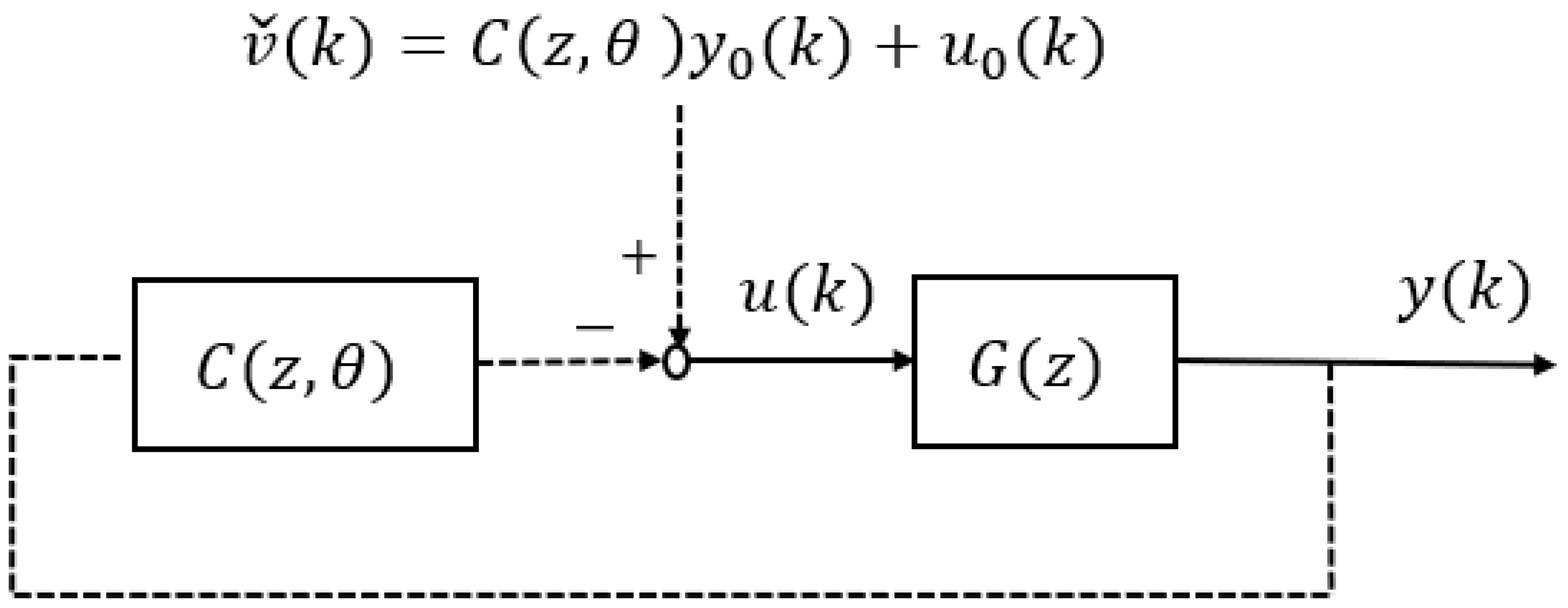
Here, we introduce the fictitious disturbance signal $\check{v}\left(k\right)$ as shown in Figure 2, which is expressed as

$$\check{v}\left(k\right)=C(z,\theta )y_0\left(k\right)+u_0\left(k\right).$$

In the z-domain, the transfer function from fictitious disturbance signal $\check{v}\left(k\right)$ to system output $\widehat{y}\left(k\right)$ is given as

$$\begin{array}{c}\hfill \check{S}(z,\theta )={\displaystyle \frac{Y\left(z\right)}{\check{V}(z,\theta )}}={\displaystyle \frac{G\left(z\right)}{1+C(z,\theta )G\left(z\right)}},\end{array}$$

(10)

where

$$\check{V}=[{\check{\mathit{v}}}_{\mathbf{0}}{\check{\mathit{v}}}_{\mathbf{1}}\dots {\check{\mathit{v}}}_{n-1}]\in {\mathbb{R}}^{n\times n}.$$

Calculating (9) and (10) yields the following results.

$$\begin{array}{c}\hfill \widehat{y}(k,\theta )=T(z,\theta )\widehat{r}\left(k\right)=C(z,\theta )\check{S}(z,\theta )\widehat{r}\left(k\right).\end{array}$$

(11)

According to the relationship between (3), (8), and (11), if $\check{v}\left(0\right)\ne 0$, the output $\widehat{\mathit{y}}$ for the arbitrary reference input $\widehat{\mathit{r}}$ and the tunable controller $C(z,\theta )$ can be estimated by

$$\begin{array}{c}\hfill \widehat{\mathit{y}}=C(z,\theta )\mathit{Y}{\check{V}}^{-1}\widehat{\mathit{r}},\end{array}$$

(12)

i.e.,

$$\begin{array}{c}\hfill \underset{\widehat{\mathit{y}}}{\underbrace{\left[\begin{array}{c}\widehat{y}\left(0\right)\\ \widehat{y}\left(1\right)\\ ⋮\\ \widehat{y}(n-1)\end{array}\right]}}=C(z,\theta )\underset{\mathit{Y}}{\underbrace{\left[\begin{array}{cccc}{y}_0\left(0\right)& 0& \dots & 0\\ y_0\left(1\right)& y_0\left(0\right)& \dots & 0\\ ⋮& ⋮& \ddots & ⋮\\ y_0(n-1)& y_0(n-2)& \dots & y_0\left(0\right)\end{array}\right]}}\\ \hfill \times {\underset{{\check{V}}^{-1}}{\underbrace{\left[\begin{array}{cccc}\check{v}\left(0\right)& 0& \dots & 0\\ \check{v}\left(1\right)& \check{v}\left(0\right)& \dots & 0\\ ⋮& ⋮& \ddots & ⋮\\ \check{v}(n-1)& \check{v}(n-2)& \dots & \check{v}\left(0\right)\end{array}\right]}}}^{-1}\underset{\widehat{\mathit{r}}}{\underbrace{\left[\begin{array}{c}\widehat{r}\left(0\right)\\ \widehat{r}\left(1\right)\\ ⋮\\ \widehat{r}(n-1)\end{array}\right]}}.\end{array}$$

The corresponding input $\widehat{\mathit{u}}$ can be estimated as

$$\begin{array}{c}\hfill \widehat{\mathit{u}}=C(z,\theta )\mathit{U}{\check{V}}^{-1}\widehat{\mathit{r}},\end{array}$$

(13)

i.e.,

$$\begin{array}{c}\hfill \underset{\widehat{\mathit{u}}}{\underbrace{\left[\begin{array}{c}\widehat{u}\left(0\right)\\ \widehat{u}\left(1\right)\\ ⋮\\ \widehat{u}(n-1)\end{array}\right]}}=C(z,\theta )\underset{\mathit{U}}{\underbrace{\left[\begin{array}{cccc}{u}_0\left(0\right)& 0& \dots & 0\\ u_0\left(1\right)& u_0\left(0\right)& \dots & 0\\ ⋮& ⋮& \ddots & ⋮\\ u_0(n-1)& u_0(n-2)& \dots & u_0\left(0\right)\end{array}\right]}}\\ \hfill \times {\underset{{\check{V}}^{-1}}{\underbrace{\left[\begin{array}{cccc}\check{v}\left(0\right)& 0& \dots & 0\\ \check{v}\left(1\right)& \check{v}\left(0\right)& \dots & 0\\ ⋮& ⋮& \ddots & ⋮\\ \check{v}(n-1)& \check{v}(n-2)& \dots & \check{v}\left(0\right)\end{array}\right]}}}^{-1}\underset{\widehat{\mathit{r}}}{\underbrace{\left[\begin{array}{c}\widehat{r}\left(0\right)\\ \widehat{r}\left(1\right)\\ ⋮\\ \widehat{r}(n-1)\end{array}\right]}}.\end{array}$$

3.2. Controller Design Method Based on Response Estimation Data

We intend to tune the controller parameters using the response estimation data described in the previous subsection. The traditional DDC method [9] only considers model-matching error, while our proposed method also accounts for the reference tracking error and input variation. In addition, designers can limit the input amplitude as needed. The following optimization problem adjusts the controller parameters:

$$\begin{array}{c}\hfill {\theta }^{*}=\underset{\theta }{\arg \min }J\left(\theta \right),\end{array}$$

(14)

where the objective function:

$$\begin{array}{cc}\hfill J\left(\theta \right)=& {\displaystyle \frac{1}{n}}\sum _{k=0}^{n-1}({\lambda }_1{(\widehat{y}\left(k\right)-y_m\left(k\right))}^2+{\lambda }_2{(r\left(k\right)-\widehat{y}\left(k\right))}^2\hfill \\ \hfill & +{\lambda }_3{(\widehat{u}\left(k\right)-\widehat{u}(k-1))}^2),\hfill \end{array}$$

subject to

$$\left\{\begin{array}{c}{\lambda }_1+{\lambda }_2+{\lambda }_3=1\hfill \\ \widehat{u}\left(k\right)\in [u_{\min },u_{\max }],\hfill \end{array}\right.$$

where ${\lambda }_1$, ${\lambda }_2$, and ${\lambda }_3$ are scalar weighting factors used to adjust the importance of each term of the function. The smaller $\widehat{y}\left(k\right)-y_m\left(k\right)$ is the higher accuracy of the model-matching. The smaller the value of $r\left(k\right)-\widehat{y}\left(k\right)$, the stronger the ability to track the target reference signal. At the same time, tracking the reference model and the reference input can improve model-matching accuracy and system response speed, and prevent the system from deviating from the reference input signal. The input variation $\mathsf{\Delta }\widehat{u}$ can smooth the input signal and suppress drastic input changes. The designer only adjusts the weight factors of the objective function to achieve the desired performance index. Moreover, actuators in actual control systems have physical limits, such as the input voltage of a motor, which cannot exceed certain values. Hence, our proposed method limits the input range to $u_{\min }$ and $u_{\max }$, the lower and upper input bounds, respectively, which the designer determined according to the control requirements. $J\left(\theta \right)$ is generally non-convex with respect to $\theta$ because both the predicted output $\widehat{y}\left(k\right)$ and the control signal $\widehat{u}\left(k\right)$ depend nonlinearly on the controller parameters. The system controller parameters are obtained by minimizing the cost function using the MATLAB R2021a nonlinear solver $\mathtt{fmincon}$.

Remark 1.

The objective function $J\left(\theta \right)$ is locally convex around the optimal controller parameters. Hence, if the initial parameters ${\theta }^0$ are chosen such that the closed-loop system is stable and the corresponding performance is reasonable, the non-linear solver $\mathtt{fmincon}$ can reliably converge to the optimal solution ${\theta }^{*}$, despite the possible non-convexity of $J\left(\theta \right)$ in the global parameter space. Refer to Section 4 for a more detailed discussion.

Here, we summarize the algorithm for the approach proposed in this paper. In addition, we also provide an overview of the FRIT algorithm to compare it with the proposed method.

The proposed data-driven design algorithm can be summarized as follows.

Algorithm 1: Proposed controller design approach.

1. Get the initial response dataset ${\{u_0\left(k\right),y_0\left(k\right)\}}_{k=0,1,\dots ,n-1}$ by a closed-loop experiment with initial controller $C(z,{\theta }^0)$.  2. Deal with the noise of the initial data by (17) and (18).  3. Estimate the response ${\{\widehat{u}\left(k\right),\widehat{y}\left(k\right)\}}_{k=0,1,\dots ,n-1}$ by (12) and (13).  4. Optimize the controller parameters by (14) using the response estimation data from step 3. The step 3 response estimation data are updated in real time during the optimization process in step 4. This process continues iteratively until the optimal controller parameters ${\theta }^{*}={[{\theta }_0^{*}{\theta }_1^{*}\dots {\theta }_{p-1}^{*}]}^T$ are determined.

The FRIT algorithm [9] for the control system depicted in Figure 1 can be described as    

Algorithm 2: FRIT approach.

1. Set the desired transfer function $M_{\mathrm{FRIT}}\left(z\right)$. Given the initial controller parameters ${\theta }^0={[{\theta }_0{\theta }_1\dots {\theta }_{q-1}]}^T$, where q is the number of the parameters. Acquire the initial input/output data $u_{ini}$ and $y_{ini}$ by an experiment.  2. The controller parameter ${\theta }^{*}$ is determined by solving the optimization problem: ${\theta }^{*}=\underset{\theta }{\arg \min }{J}_{\mathrm{FRIT}}\left(\theta \right)$, objective function: $J_{\mathrm{FRIT}}\left(\theta \right)={\displaystyle \frac{1}{n}}{\sum }_{k=0}^{n-1}{\left(y_{ini}\left(k\right)-M_{\mathrm{FRIT}}\left(z\right)\tilde{r}\left(k\right)\right)}^2$ where $\tilde{r}\left(k\right)=C{(z,\theta )}^{-1}{u}_{ini}\left(k\right)+y_{ini}\left(k\right)$ is the fictitious reference signal.

A comparison of the Algorithms 1 and 2 shows that the objective function of the FRIT method considers only the tracking performance of the reference model M. In contrast, our method simultaneously considers reference model tracking performance, reference input tracking performance, and input signal smoothing. The designer can adjust the weighting parameters to optimize multiple performance indices rather than only matching the reference model.

3.3. Dealing with Noise

In industrial applications, actual experiments are affected by noise, leading to noisy initial data. In this section, a denoising method is introduced. When the initial data are corrupted by noise, they are first denoised, and then the controller is designed following the procedure described in Section 3.2.

The input and output with the noise of the closed-loop system are expressed as

$$\begin{array}{cc}\hfill u_0\left(k\right)& ={\displaystyle \frac{C(z,\theta )}{1+G\left(z\right)C(z,\theta )}}(r\left(k\right)-Q\left(k\right)),\hfill \\ \hfill y_0\left(k\right)& ={\displaystyle \frac{G\left(z\right)C(z,\theta )r\left(k\right)+Q\left(k\right)}{1+G\left(z\right)C(z,\theta )}},\hfill \end{array}$$

where $u_0\left(k\right)$ and $y_0\left(k\right)$ are the initial input and output data, respectively, with Gaussian white noise $Q\left(k\right)$.

The total variation denoising method is introduced to address the noise of the initial input/output data [18,30]. The regularization of the $L_2$ norm is more suitable for dealing with time-series data, so the denoising problem can be described as follows:

$$\begin{array}{cc}\hfill & \underset{{\mathit{u}}_{\mathit{w}}}{min}\Vert {\mathit{u}}_{\mathit{w}}-{\mathit{u}}_{\mathbf{0}}{\Vert }_2^2+\mathsf{\Lambda } {\Vert H{\mathit{u}}_{\mathit{w}}\Vert }_2^2,\hfill \end{array}$$

(15)

$$\begin{array}{cc}\hfill & \underset{{\mathit{y}}_{\mathit{w}}}{min}\Vert {\mathit{y}}_{\mathit{w}}-{\mathit{y}}_{\mathbf{0}}{\Vert }_2^2+\mathsf{\Lambda } {\Vert H{\mathit{y}}_{\mathit{w}}\Vert }_2^2,\hfill \end{array}$$

(16)

where ${\mathit{u}}_{\mathit{w}}={[u_w\left(0\right)u_w\left(1\right)\dots u_w(n-)]}^T\in {\mathbb{R}}^n$ and ${\mathit{y}}_{\mathit{w}}={[y_w\left(0\right)y_w\left(1\right)\dots y_w(n-)]}^T\in {\mathbb{R}}^n$ represent the denoised finite-length control input and output sequence. ${\mathit{u}}_{\mathbf{0}}={[u_0\left(0\right)u_0\left(1\right)\dots u_0(n-)]}^T\in {\mathbb{R}}^n$ and ${\mathit{y}}_{\mathbf{0}}={[y_0\left(0\right)y_0\left(1\right)\dots y_0(n-)]}^T\in {\mathbb{R}}^n$ represent the initial input and output sequences with noise. $\Vert {\mathit{u}}_{\mathit{w}}-{\mathit{u}}_{\mathbf{0}}{\Vert }_2^2$ and $\Vert {\mathit{y}}_{\mathit{w}}-{\mathit{y}}_{\mathbf{0}}{\Vert }_2^2$ are the data fitting terms, ensuring that the denoised data is close to the initial data. H denotes the discrete difference matrix as below:

$$H=\left[\begin{array}{ccccc}-1& 1& 0& \dots & 0\\ 0& -1& 1& \dots & 0\\ ⋮& ⋮& \ddots & \ddots & ⋮\\ 0& \dots & 0& -1& 1\\ 0& \dots & 0& 0& 0\end{array}\right]\in {\mathbb{R}}^{n\times n}.$$

$\Vert H{\mathit{y}}_{\mathit{w}}{\Vert }_2^2$ is the regularization term that limits the signal variation for smoothing. The value of the regularization parameter $\mathsf{\Lambda }$ determines the degree of denoising.

$\mathsf{\Lambda }\to 0$: Almost no denoising. The denoise data $\{{\mathit{u}}_{\mathit{w}},{\mathit{y}}_{\mathit{w}}\}$ are almost equal to the initial data $\{{\mathit{u}}_{\mathbf{0}},{\mathit{y}}_{\mathbf{0}}\}$.

$\mathsf{\Lambda }\to \infty$: Excessive denoising makes the output overly smooth.

Solving (15) and (16) by the least squares method yields

$$\begin{array}{cc}\hfill {\mathit{y}}_{\mathit{w}}^{*}& ={\left(I_n+\mathsf{\Lambda }{H}^{T}H\right)}^{-1}{\mathit{y}}_{\mathbf{0}},\hfill \end{array}$$

(17)

$$\begin{array}{cc}\hfill {\mathit{u}}_{\mathit{w}}^{*}& ={\left(I_n+\mathsf{\Lambda }{H}^{T}H\right)}^{-1}{\mathit{u}}_{\mathbf{0}}.\hfill \end{array}$$

(18)

For now, we can handle the noise in the initial input/output data by (17) and (18).

4. Simulation Example

We use a dead-time control system for numerical simulation because many industrial systems have delays.

The controlled plant is

$$\begin{array}{cc}\hfill G\left(z\right)& =z\left(G\right(s\left)\right),\hfill \end{array}$$

where

$$\begin{array}{cc}\hfill G\left(s\right)& ={\displaystyle \frac{s+6}{s^2+6s+3}}{e}^{-L_{1}s},\hfill \end{array}$$

and $L_1>0$ is the constant dead-time. The reference model for the proposed method is given by

$$\begin{array}{cc}\hfill M\left(z\right)& =z\left(M\right(s\left)\right),\hfill \end{array}$$

where

$$\begin{array}{cc}\hfill M\left(s\right)& ={\displaystyle \frac{1}{0.95s+1}}{e}^{-L_{2}s},\hfill \end{array}$$

and $L_2>0$ is the constant dead-time.

The reference model $M\left(z\right)$ is a first-order plus dead-time (FOPDT) system because it can effectively approximate a wide range of practical industrial processes while keeping the model simple. The choice of the reference model usually depends on the desired closed-loop performance, such as rise time, settling time, and overshoot, which can be intuitively tuned through the model parameters. Although the second-order model could also be used, the FOPDT model provides a good balance between precision, design simplicity, and robustness, which makes it suitable for the proposed control framework.

The structure of the controller is expressed as

$$C(z,\theta )=\left[\begin{array}{ccc}1& {\displaystyle \frac{1}{1-z^{-1}}}& {\displaystyle \frac{z^{-1}}{1-z^{-1}}}\end{array}\right]{\left[\begin{array}{ccc}{\theta }_0& {\theta }_1& {\theta }_2\end{array}\right]}^T.$$

In the simulation, we set the sampling time $T_s=0.5\mathrm{s}$, the total simulation time $T=60\mathrm{s}$, the dead-time $L_1=0.15\mathrm{s}$ and $L_2=0.2\mathrm{s}$.

First, we consider the ideal noise-free situation. We verify the effectiveness of the response estimation method. Set the initial controller parameters ${\theta }^0={\left[0.37-0.120.33\right]}^T$, and the controller parameters after adjustment are ${\theta }^{*}={\left[0.850.230.02\right]}^T$. To verify that the response estimation method is effective for different forms of reference input signals, here we set the reference input signals to be the following three waveforms:

(1) Unit step signal: $r\left(k\right)=1$.

(2) Square wave: $r\left(k\right)=sgn(sin(0.2\pi k\left)\right)$.

(3) Sine wave: $r\left(k\right)=sin\left(0.2\pi k\right)+1$.

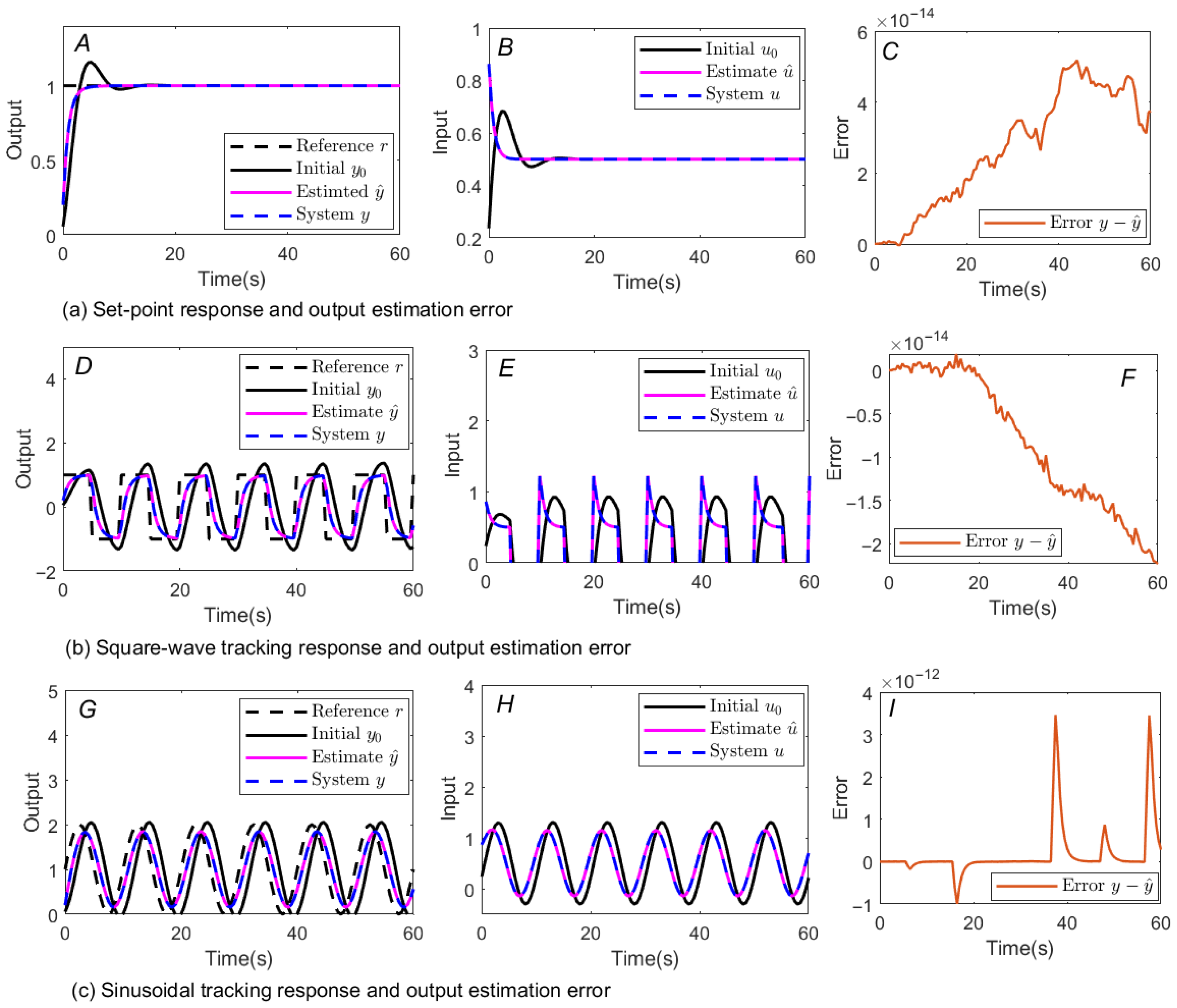
The closed-loop responses and output estimation error for all types of reference signals (step, square, and sine) are shown in Figure 3. In Figure 3A,D,G, we can see the good tracking performance between the actual system output y and the estimated output $\widehat{y}$, where the estimated response $\widehat{y}$ (red solid line) is consistent with the system output $y\left(k\right)$ (blue dashed line), thus verifying the effectiveness of the proposed response estimation method. In addition, Figure 3C,F,I show that the error between the estimated and actual system outputs is minimal and can be ignored. We can demonstrate that the estimated response closely aligns with the actual output of the control system. Furthermore, the mean squared error (MSE) values can evaluate the magnitude of the difference between the estimated and actual output values, where $\mathrm{MSE}={\displaystyle \frac{1}{N}}{\sum }_{k=1}^N{\left(y\left(k\right)-\widehat{y}\left(k\right)\right)}^2$. In Figure 3A,D,G, the MSE of the three reference input cases are ${\mathrm{MSE}}_1=9.7922\times {10}^{-28}$, ${\mathrm{MSE}}_2=1.2679\times {10}^{-28}$, and ${\mathrm{MSE}}_3=4.4888\times {10}^{-25}$, respectively. These MSE values are very small and almost negligible. This indicates that the response estimation method is valid when the step response, square wave, and sine wave are reference input signals, respectively.

Next, we discuss the effectiveness of the controller design method based on response estimation data. The reference signal $r\left(k\right)$ is set here and used for subsequent simulations until the noise simulation section.

$$r\left(k\right)=\left\{\begin{array}{cc}1.0,\hfill & 0\le k\le 20\hfill \\ 2.0,\hfill & 20\le k\le 40\hfill \\ 1.5,\hfill & 40\le k\le 60.\hfill \end{array}\right.$$

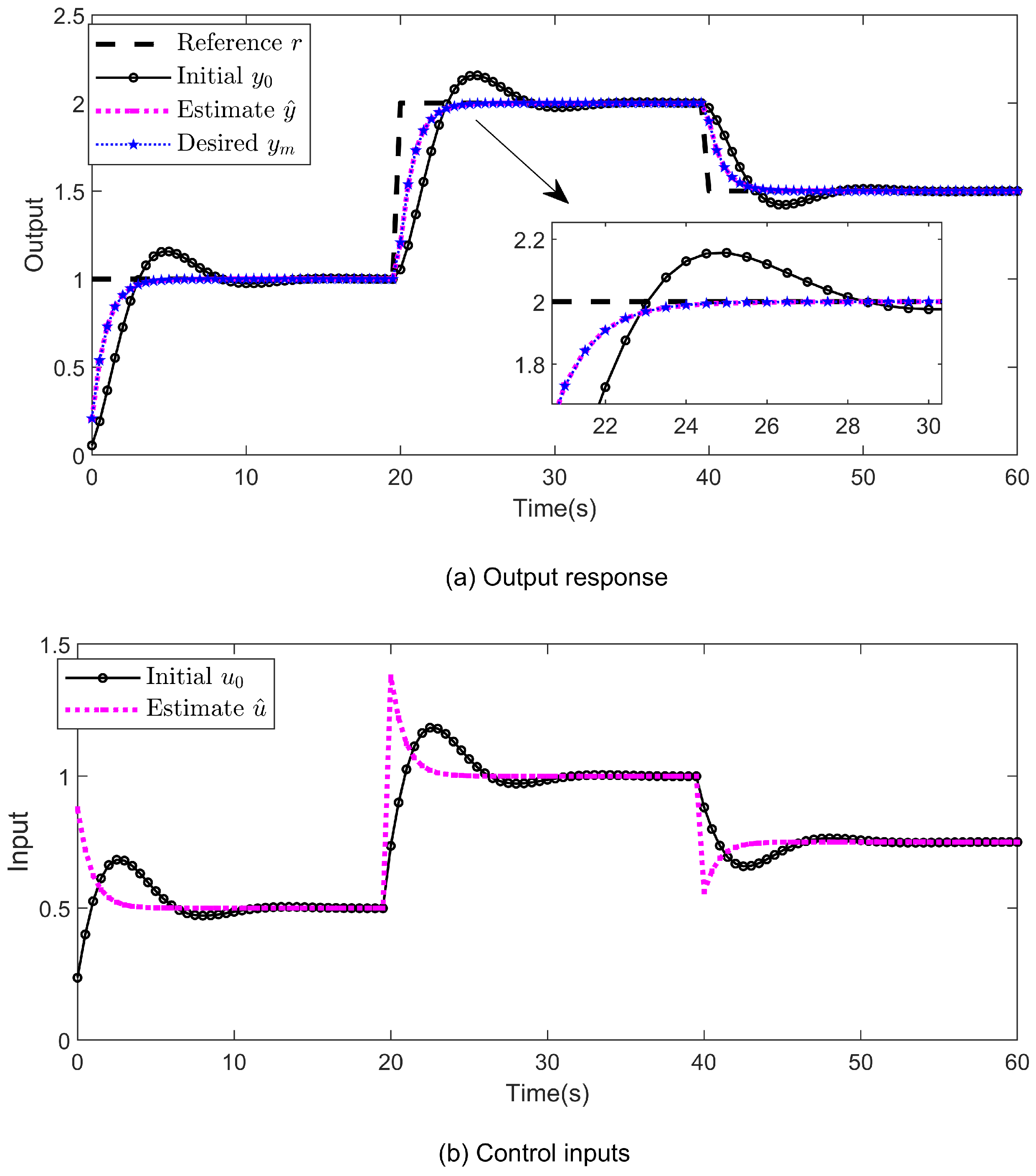
We take the initial controller parameters ${\theta }^0={\left[0.37-0.120.33\right]}^T$. The tuned controller parameters ${\theta }^{*}={\left[0.9191-0.18050.0811\right]}^T$ when ${\lambda }_1=1$, ${\lambda }_2=0$, and ${\lambda }_3=0$ and without input constraints. As shown in Figure 4, the estimated output curve (red dashed line) of the proposed tuning method is consistent with the desired reference output curve (blue dashed line). In addition, the optimized estimated output plot has a shorter rise time than the initial output (black solid line), and its values converge quickly.

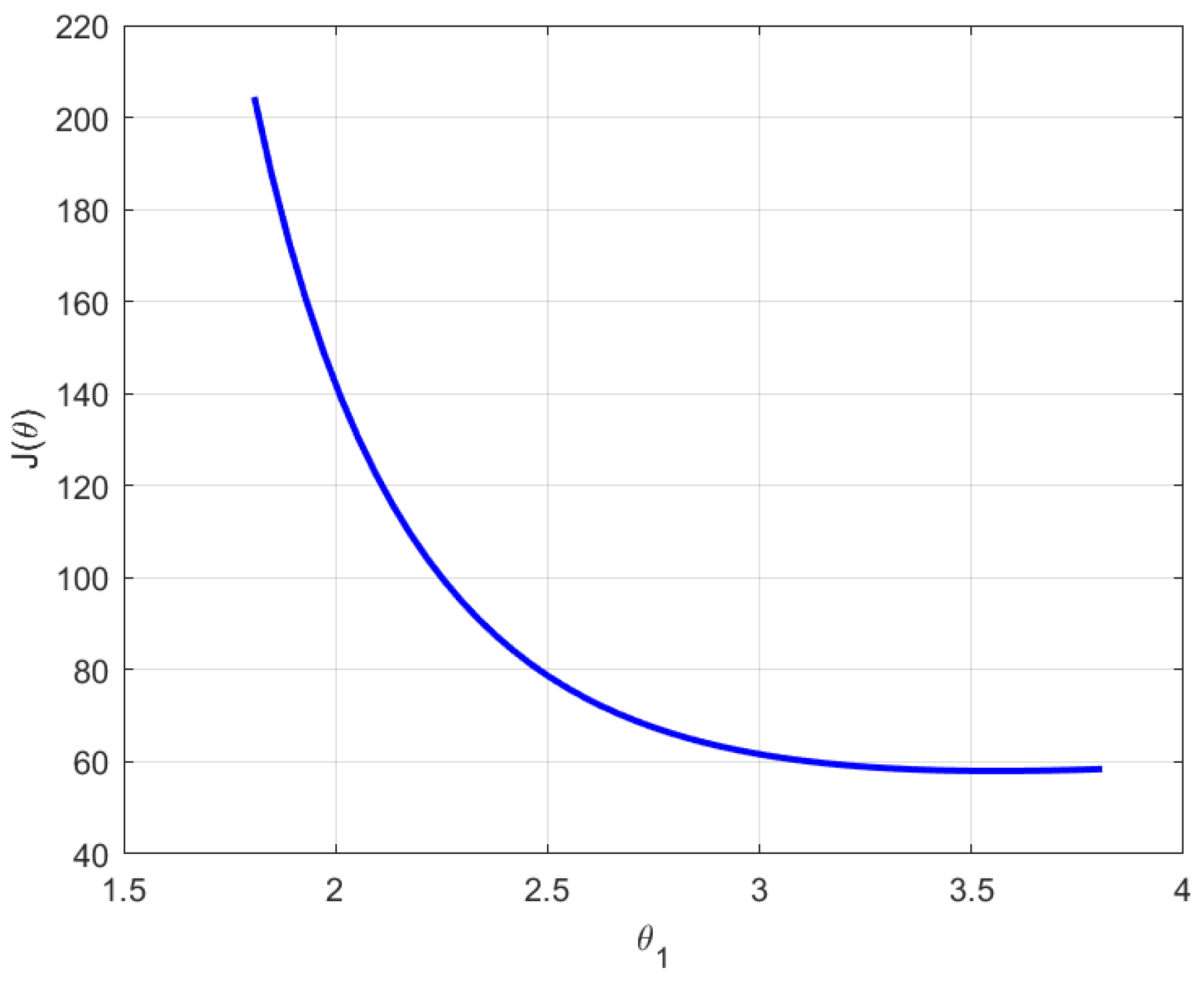
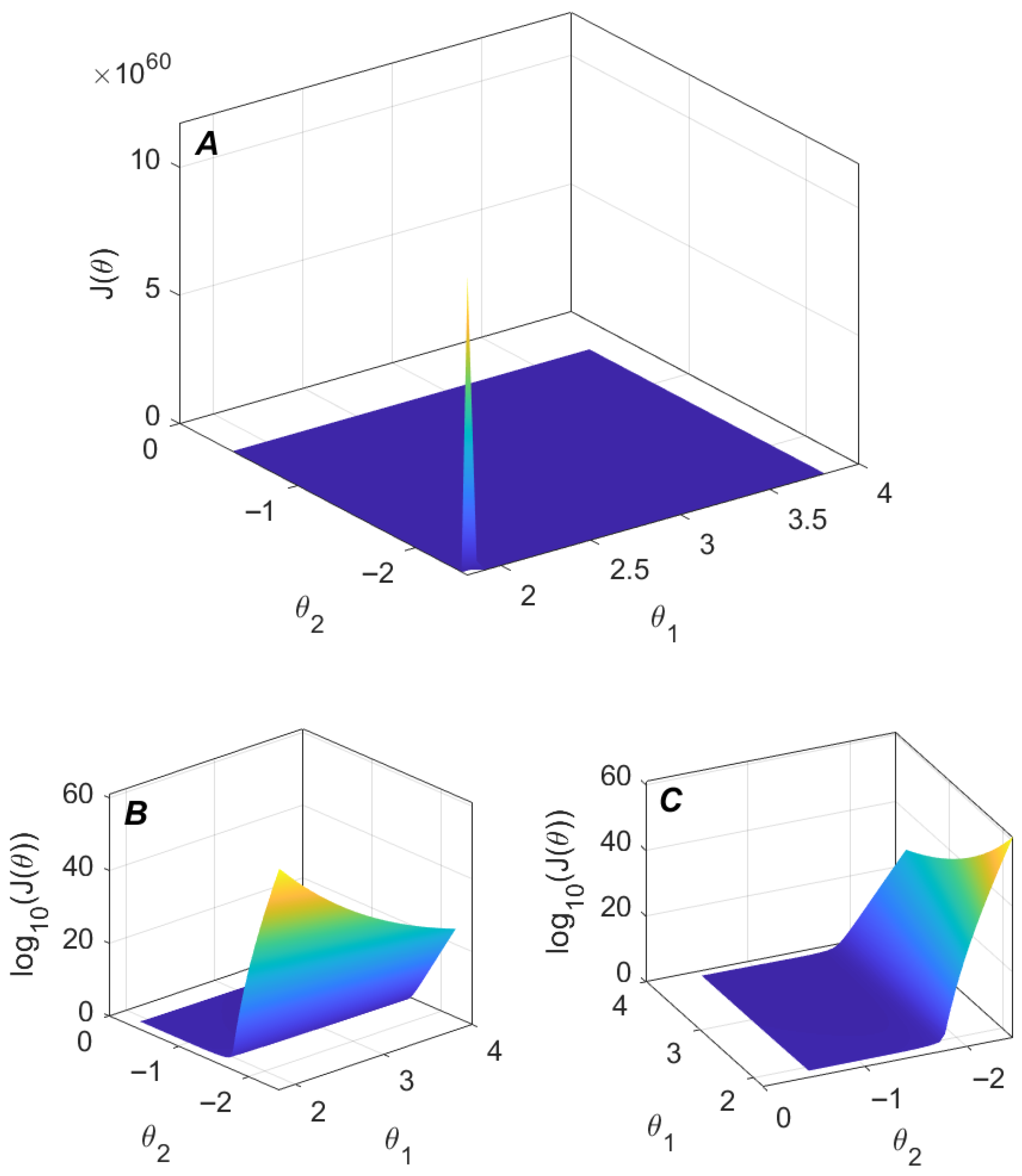
To further analyze the characteristics of the objective function $J\left(\theta \right)$ and its impact on the convergence of optimization, we examine the one-dimensional and two-dimensional profiles of $J\left(\theta \right)$ around the optimal controller parameters. Figure 5 shows the variation of the objective function with respect to the parameter ${\theta }_1$, with the other parameters fixed at their optimal values. The curve is smooth and monotonically decreasing toward the optimal solution, indicating local convexity in this parameter direction and supporting the reliable convergence of the proposed optimization method. Figure 6 presents the surface of the objective function $J({\theta }_1,{\theta }_2)$ around the optimal solution, with ${\theta }_3$ fixed at its optimal value. Figure 6A shows the surface on a linear scale, where a sharp peak is observed near the optimum. Figure 6B,C illustrate the same surface on a logarithmic scale, offering a clearer view of the overall landscape. Although an isolated sharp peak remains in regions far from the optimal point, the surface near the optimal point exhibits a flat bottom. This indicates that the optimization problem is locally convex around the optimum, allowing the nonlinear solver to converge reliably despite potential non-convexity in the global parameter space.

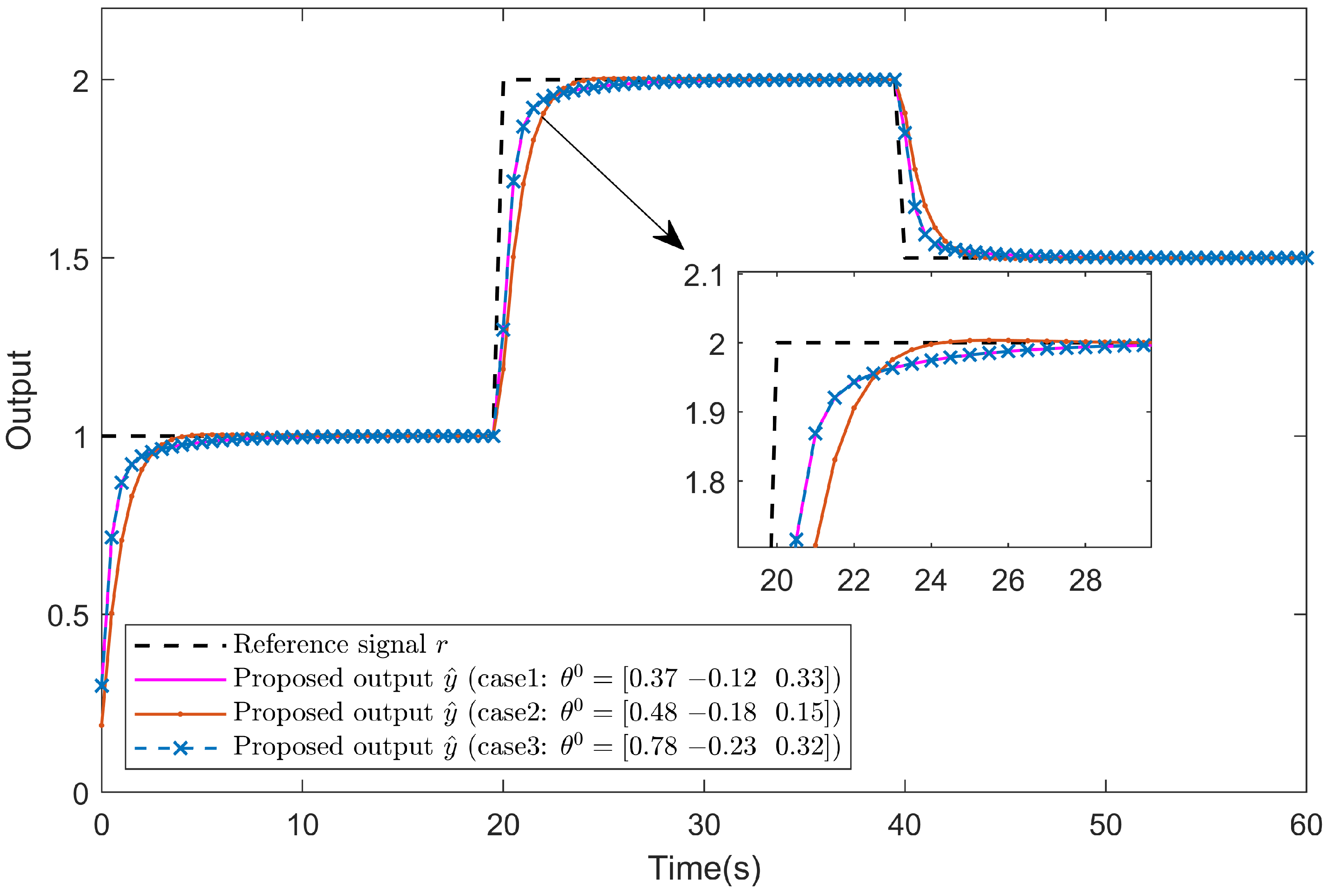
To investigate the influence of the initial controller parameters on convergence, several simulations were performed with different sets of initial parameters: case 1: ${\theta }^0={\left[0.37-0.120.33\right]}^{\mathrm{T}}$, case 2: ${\theta }^0={\left[0.48-0.180.15\right]}^{\mathrm{T}}$, and case 3: ${\theta }^0={\left[0.78-0.230.32\right]}^{\mathrm{T}}$. Figure 7 compares the corresponding closed-loop responses. In all cases, the optimization procedure consistently converges to steady-state responses. Although the transient behaviors exhibit slight differences at the beginning, all trajectories smoothly converge toward the reference signal r, demonstrating that the proposed optimization method is robust to the choice of ${\theta }^0$. This observation further confirms that the local convexity of the cost function $J\left(\theta \right)$ around the optimum ensures a reliable convergence of the nonlinear solver.

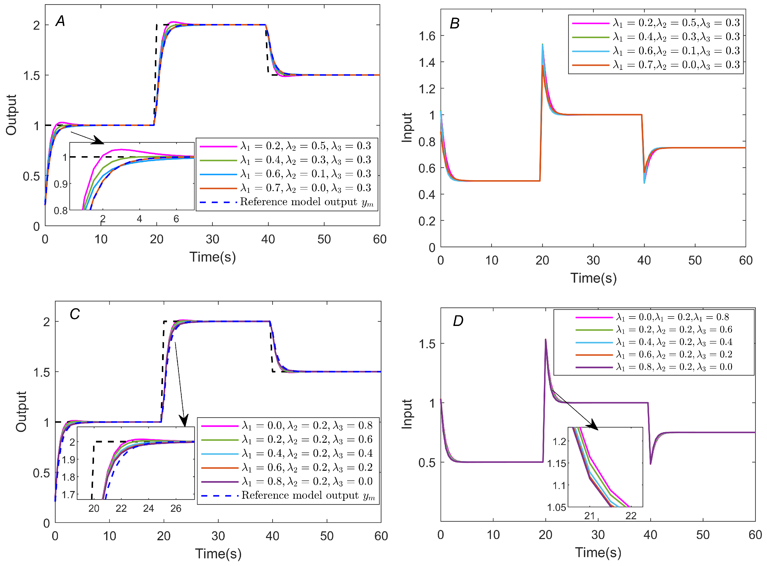
Figure 8 represents the effect of adjusting different weight factors of ${\lambda }_1$, ${\lambda }_2$, and ${\lambda }_3$ on the input/output results. The solid and blue dashed lines indicate the trajectories of the estimated and reference model outputs, respectively. When adjusting ${\lambda }_1$ and ${\lambda }_2$ with fixed ${\lambda }_3=0.3$, the smaller ${\lambda }_1$ and the larger ${\lambda }_2$, the response of the system is shorter in rise time; the larger ${\lambda }_1$ and the smaller ${\lambda }_2$, the longer the rise time, and the estimated output is closer to the output of the reference model. When adjusting ${\lambda }_1$ and ${\lambda }_3$ while fixing ${\lambda }_2=0.2$, the smaller ${\lambda }_1$ and the larger ${\lambda }_3$, the control input is smoother; however, the tracking performance of the reference model degrades; the larger ${\lambda }_1$ and the smaller ${\lambda }_3$, the more accurately the output signal tracks the reference model signal but causes abrupt changes for the control input. There is a trade-off relationship between them: ${\lambda }_1$ affects the reference tracking performance of the system and the response speed, ${\lambda }_2$ affects the model-matching accuracy, and ${\lambda }_3$ affects the input control smoothness of the system. Designers can combine application scenarios to analyze and set appropriate weight parameters.

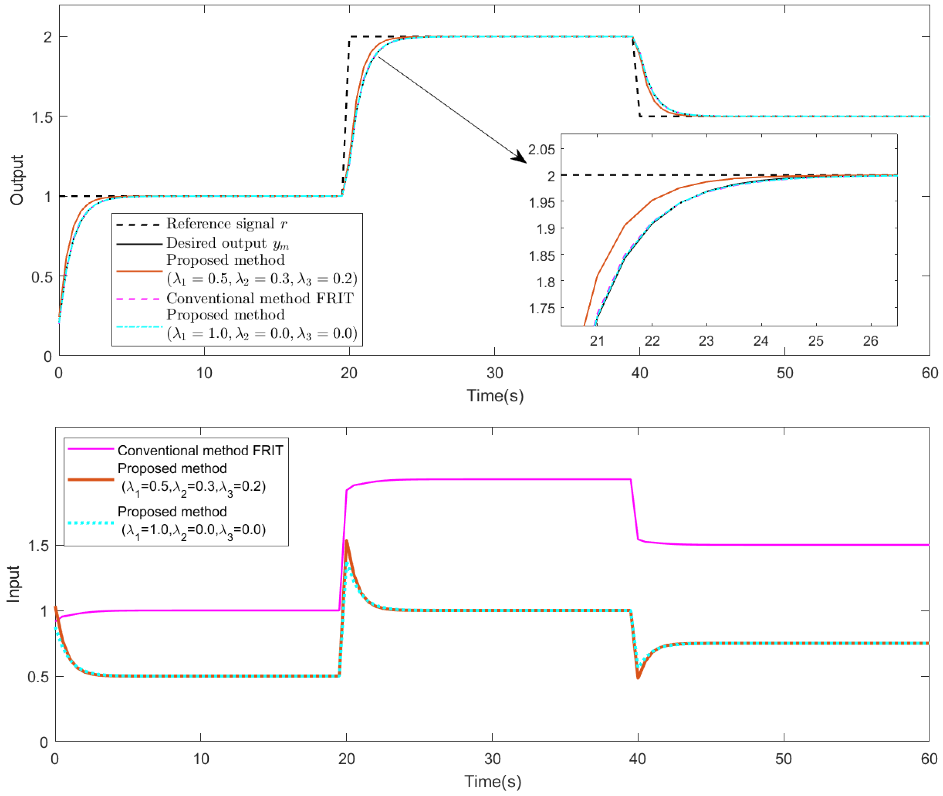
Now, we set $\tau =0.95$ and $L_3=0.2$ to compare with the FRIT method. As shown in Figure 9, the proposed method can meet design requirements by adjusting the weighting factors ${\lambda }_1$, ${\lambda }_2$, and ${\lambda }_3$. In contrast, the traditional FRIT method only considers reducing the reference output error when tuning the controller parameters.

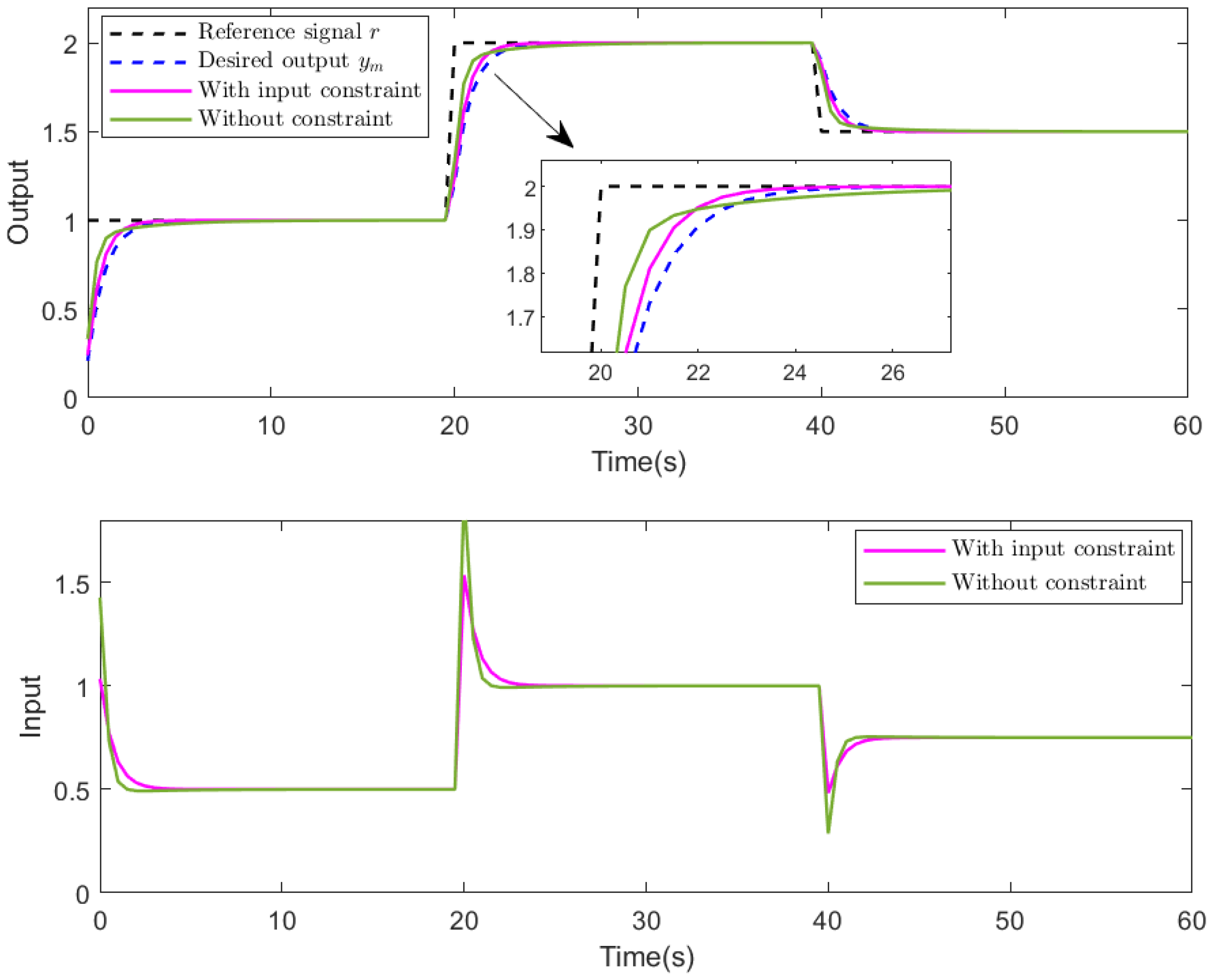
In control system design, it is sometimes necessary to consider input constraints. Here, the control input limit is $-2\le u\le 2$ compared to the case without input constraint. Set ${\lambda }_1=0.5$, ${\lambda }_2=0.3$, and ${\lambda }_3=0.2$. The input/output results after tuning are shown in Figure 10. When the input limit is applied, the control input is reduced and remains within the given range, while the output response converges faster.

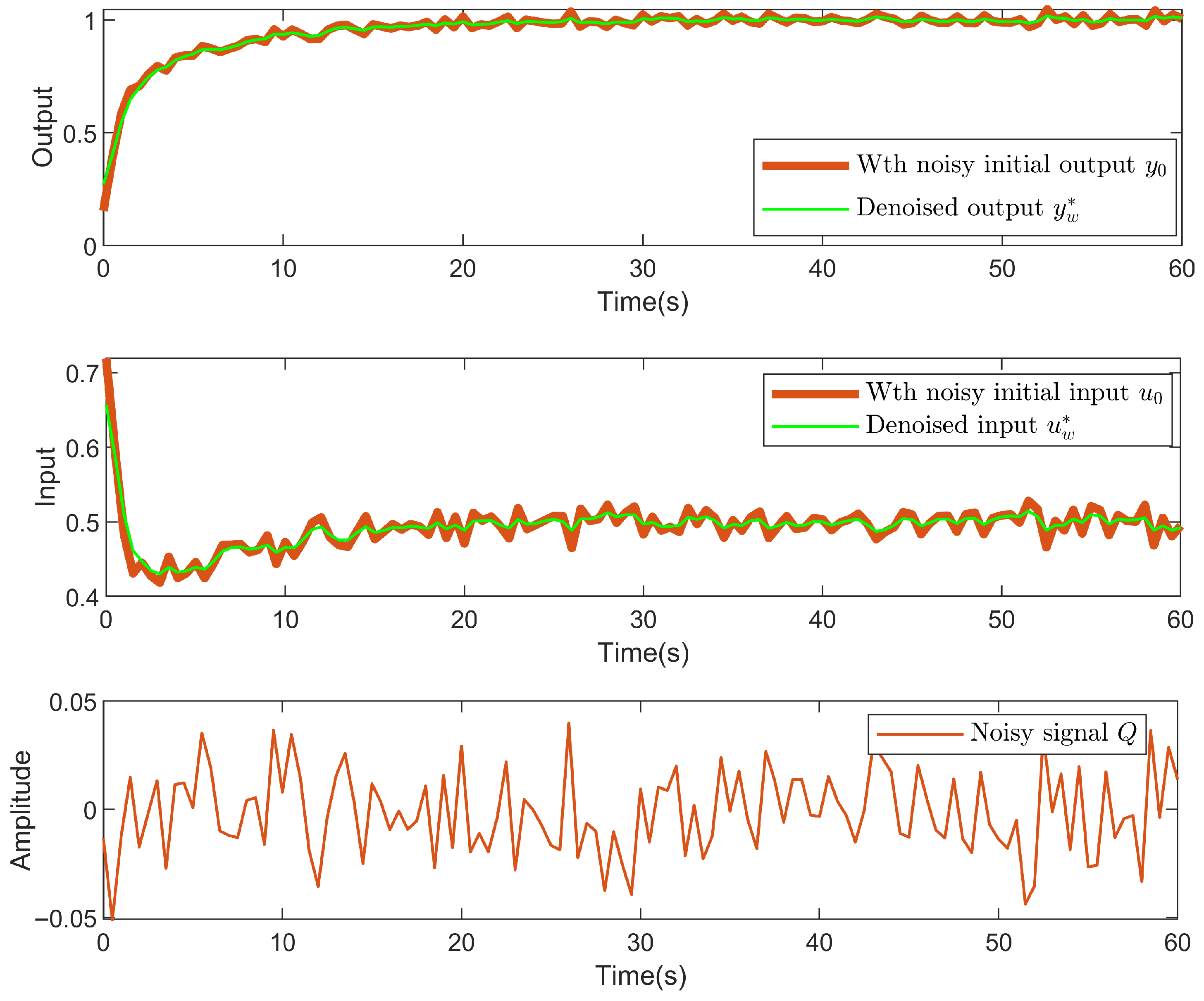
Lastly, we discuss the case where the input/output signal is affected by noise. Here, the noise is Gaussian white noise with a variance of 0.005 and a signal-to-noise ratio $\mathrm{SNR}=15$. The initial controller parameters given are ${\theta }^0={\left[0.97-0.120.21\right]}^T$. The reference input signal is $r\left(k\right)=1$. To deal with the noise in the initial dataset, set $\mathsf{\Lambda }=0.9$. The results of noise dealing are shown in Figure 11. Let the weight factors ${\lambda }_1=0.3$, ${\lambda }_2=0$, and ${\lambda }_3=0.7$, and the input without limits. The results of the proposed method after tuning are shown in Figure 12. The black solid line represents the initial input/output data with noise, the red solid line represents the actual input/output after tuning (with noise), and the green solid line represents the results of the proposed method after tuning (denoised data). The output of the proposed method can track the output of the reference model. Figure 11 and Figure 12 demonstrate the effectiveness of the proposed denoising and controller design methods.

5. Conclusions

This study introduces a novel data-driven approach based on response estimation technology for linear systems. We can predict the input/output response of the tuned controller before implementing it on the machine, thereby avoiding machine damage and reducing the experimental costs. The designer tunes the controller by adjusting the weight factors to balance tracking performance, response speed, and smoothness. The simulation example verifies the proposed method. However, the response estimation method is currently used only for SISO LTI systems. We plan to expand the response estimation method to MIMO LTI systems and nonlinear systems in future work. Furthermore, we will use the data-driven control method proposed in this paper for actual systems and extend it to 2-DOF systems.

References

1. Ren, W.; Duan, G.R.; Li, P.; Kong, H. Set-Based Fault-Tolerant Control for Continuous-Time Nonlinear Systems: A Fully Actuated System Approach. IEEE/ASME Trans. Mechatronics 2025, 1–12. [Google Scholar] [CrossRef]
2. Ren, W.; Duan, G.R.; Li, P.; Kong, H. Observer-Based Active Fault/Disturbance Compensated Control for Fully Actuated Systems. Sci. China Inf. Sci. 2025. [Google Scholar]
3. Hou, Z.S.; Wang, Z. From model-based control to data-driven control: Survey, classification and perspective. Inf. Sci. 2013, 235, 3–35. [Google Scholar] [CrossRef]
4. Precup, R.E.; Roman, R.C.; Safaei, A. Data-Driven Model-Free Controllers; CRC Press: Boca Raton, FL, USA, 2021. [Google Scholar]
5. Campi, M.C.; Lecchini, A.; Savaresi, S.M. Virtual reference feedback tuning: A direct method for the design of feedback controllers. Automatica 2002, 38, 1337–1346. [Google Scholar] [CrossRef]
6. Lecchini, A.; Campi, M.C.; Savaresi, S.M. Virtual reference feedback tuning for two degree of freedom controllers. Int. J. Adapt. Control Signal Process. 2002, 16, 355–371. [Google Scholar] [CrossRef]
7. Hjalmarsson, H.; Gevers, M.; Gunnarsson, S.; Lequin, O. Iterative feedback tuning: Theory and applications. IEEE Control Syst. Mag. 1998, 18, 26–41. [Google Scholar]
8. Karimi, A.; Van Heusden, K.; Bonvin, D. Non-iterative data-driven controller tuning using the correlation approach. In Proceedings of the 2007 European control conference (ECC), Kos, Greece, 2–5 July 2007; IEEE: Piscataway, NJ, USA, 2007; pp. 5189–5195. [Google Scholar]
9. Soma, S.; Kaneko, O.; Fujii, T. A new method of controller parameter tuning based on input-output data–Fictitious Reference Iterative Tuning (FRIT)–. IFAC Proc. Vol. 2004, 37, 789–794. [Google Scholar] [CrossRef]
10. Kaneko, O.; Yamashina, Y.; Yamamoto, S. Fictitious reference tuning of the feed-forward controller in a two-degree-of-freedom control system. SICE J. Control. Meas. Syst. Integr. 2011, 4, 55–62. [Google Scholar] [CrossRef]
11. Vrančić, D.; Moura Oliveira, P.; Bisták, P.; Huba, M. Model-Free VRFT-Based Tuning Method for PID Controllers. Mathematics 2023, 11, 715. [Google Scholar] [CrossRef]
12. Yonezawa, A.; Yonezawa, H.; Yahagi, S.; Kajiwara, I. Practical one-shot data-driven design of fractional-order PID controller: Fictitious reference signal approach. ISA Trans. 2024, 152, 208–216. [Google Scholar] [CrossRef]
13. Sakatoku, T.; Yubai, K.; Yashiro, D.; Komada, S. Constraints to Guarantee Gain and Phase Margins for Data-Driven Controller Tuning Methods. J. Mar. Sci. Technol. 2020, 28, 8. [Google Scholar]
14. Wildhagen, S.; Berberich, J.; Hertneck, M.; Allgöwer, F. Data-driven analysis and controller design for discrete-time systems under aperiodic sampling. IEEE Trans. Autom. Control 2022, 68, 3210–3225. [Google Scholar] [CrossRef]
15. Mattera, G.; Caggiano, A.; Nele, L. Optimal data-driven control of manufacturing processes using reinforcement learning: An application to wire arc additive manufacturing. J. Intell. Manuf. 2025, 36, 1291–1310. [Google Scholar] [CrossRef]
16. Seuret, A.; Tarbouriech, S. Robust data-driven control design for linear systems subject to input saturation. IEEE Trans. Autom. Control 2024, 69, 6191–6198. [Google Scholar] [CrossRef]
17. Shen, H.; Peng, C.; Yan, H.; Xu, S. Data-driven near optimization for fast sampling singularly perturbed systems. IEEE Trans. Autom. Control 2024, 69, 4689–4694. [Google Scholar] [CrossRef]
18. Yahagi, S.; Kajiwara, I. Direct tuning of the data-driven controller considering closed-loop stability based on a fictitious reference signal. Meas. Control 2021, 54, 1026–1042. [Google Scholar] [CrossRef]
19. Sakai, T.; Yahagi, S.; Kajiwara, I. Two-degree-of-freedom controller design based on a data-driven estimation approach. IEEE Access 2022, 10, 120475–120491. [Google Scholar] [CrossRef]
20. Sakatoku, T.; Yubai, K.; Yashiro, D.; Komada, S. Data-Driven Controller Tuning with Closed-Loop Response Estimation. IEEJ Trans. Electr. Electron. Eng. 2021, 16, 1397–1406. [Google Scholar] [CrossRef]
21. Yang, R.; Yubai, K.; Komada, S.; Yashiro, D.; Ren, W. Response Estimation and Reference Model-free Controller Design Approach for 2-DOF Control Systems. In Proceedings of the 2024 3rd Conference on Fully Actuated System Theory and Applications (FASTA), Shenzhen, China, 10–12 May 2024; IEEE: Piscataway, NJ, USA, 2024; pp. 314–318. [Google Scholar]
22. Sato, T.; Sakai, Y.; Kawaguchi, N.; Hara, M.; Matsuki, T.; Takahashi, M.; Arrieta, O.; Vilanova, R. Data-driven response estimation-based tuning and its validation using a ball-and-beam system. In Proceedings of the 2023 IEEE 28th International Conference on Emerging Technologies and Factory Automation (ETFA), Sinaia, Romania, 12–15 September 2023; IEEE: Piscataway, NJ, USA, 2023; pp. 1–7. [Google Scholar]
23. Kaneko, O.; Nakamura, T.; Ikezaki, T. A New Approach to Update of Feedfoward Controller in the Two-degree-of-freedom Control System—A Proposal of Estimated Response Iterative Tuning (ERIT)—. J. Soc. Instrum. Control Eng. 2018, 54, 857–864. (In Japanese) [Google Scholar] [CrossRef]
24. Yahagi, S.; Kajiwara, I. One-Shot Data-Driven Design for Feedback Controller and Reference Model With BIBO Stability. IEEE Access 2024, 12, 147882–147893. [Google Scholar] [CrossRef]
25. Yahagi, S.; Kajiwara, I. Direct tuning of PID controller and reference model with input constraint. In Proceedings of the 2021 21st International Conference on Control, Automation and Systems (ICCAS), Jeju, Republic of Korea, 12–15 October 2021; IEEE: Piscataway, NJ, USA, 2021; pp. 1424–1429. [Google Scholar]
26. Nakatani, Y.; Kinoshita, T.; Yamamoto, T. Design of a Data-Driven Control System based on Reference Model using Predicted Input/Output Responses. J. Robot. Netw. Artif. Life 2021, 8, 170–174. [Google Scholar] [CrossRef]
27. Kurokawa, R.; Sato, T.; Vilanova, R.; Konishi, Y. Closed-loop data-driven trade-off PID control design. IFAC-PapersOnLine 2018, 51, 244–249. [Google Scholar] [CrossRef]
28. Nishiya, Y.; Kinoshita, T.; Yamamoto, T. Design of a Data-Driven Controller based on Estimated I/O Data using Open-Loop Data. J. Adv. Artif. Life Robot. 2021, 2, 48–52. [Google Scholar]
29. Tasaka, K.; Kano, M.; Ogawa, M.; Masuda, S.; Yamamoto, T. Direct PID tuning from closed-loop data and its application to unstable processes. Trans. Inst. Syst. Control Inf. Eng. 2009, 22, 137–144. (In Japanese) [Google Scholar]
30. You, Y.L.; Kaveh, M. Fourth-order partial differential equations for noise removal. IEEE Trans. Image Process. 2000, 9, 1723–1730. [Google Scholar] [CrossRef]
Figure 1. Block diagram of control system.
Actuators 14 00521 g001
Figure 2. Conceptual diagram of the fictitious disturbance signal.
Actuators 14 00521 g002
Figure 3. The results of responses with different reference input signals and the output error between the actual system output and the estimated output. (a) Set-point response (A,B) and output estimation error (C), (b) square-wave tracking response (D,E) and output estimation error (F), and (c) sinusoidal tracking response (G,H) and output estimation error (I).
Actuators 14 00521 g003
Figure 4. The desired and estimated response of the closed-loop system. (a) Output response: initial output y 0 (black solid line), proposed estimate output y ^ (red dashed line), and desired output y m (blue dashed line); (b) control inputs: initial control input u 0 (black solid line), and proposed estimate input u ^ (red dashed line).
Actuators 14 00521 g004
Figure 5. Objective function profile along θ 1 around the optimal solution.
Actuators 14 00521 g005
Figure 6. Surface of the objective function J ( θ ) near the optimal solution. (A) Linear-scale surface showing a sharp peak near the optimum; (B,C) log-scaled surface for clearer visualization of the global shape.
Actuators 14 00521 g006
Figure 7. Closed-loop responses under different initial controller parameters: case 1 ( θ 0 = [ 0.37 0.12 0.33 ] T ), case 2 ( θ 0 = [ 0.48 0.18 0.15 ] T ), and case 3 ( θ 0 = [ 0.78 0.23 0.32 ] T ).
Actuators 14 00521 g007
Figure 8. Comparison of results for different weighting factors λ 1 , λ 2 , and λ 3 . (A): proposed estimated outputs y ^ (solid lines) when fixed λ 3 ; reference model output y m (blue dashed line). (B): proposed estimated inputs u ^ when fixed λ 3 . (C): proposed estimated outputs y ^ (solid lines) when fixed λ 2 ; reference model output y m (blue dashed line). (D): proposed estimated inputs u ^ when fixed λ 2 .
Actuators 14 00521 g008
Figure 9. Comparison with the conventional FRIT method [9]. The upper and lower plots show the output response and control input, respectively. The black dashed line represents the reference input signal r, the solid black line indicates the desired output y m , the red line is the output and input obtained by the conventional FRIT method, and the solid orange and dashed blue lines correspond to the estimated outputs obtained by the proposed method.
Actuators 14 00521 g009
Figure 10. Comparison of results with and without input constraints. Each subfigure contains: top-response for with input constraint ( 2 u 2 ) and without constraint using the proposed method, where the blue dashed line is the desired output y m and the black dashed line is the reference signal r; bottom-control input of the proposed method with input constraint ( 2 u 2 ) and without constraint.
Actuators 14 00521 g010
Figure 11. The effect of noise handling. Output response (upper), control input (middle), and Gaussian white noise (lower).
Actuators 14 00521 g011
Figure 12. The upper and lower plots show the output response and the control input, respectively. The black solid line represents the initial input/output with noise; the red solid line indicates the tuned actual system input/output; the green solid line represents the estimated input/output obtained by the proposed method; the black dashed line represents the reference signal r; and the blue dashed line corresponds to the reference model output y m .
Actuators 14 00521 g012
Disclaimer/Publisher’s Note: The statements, opinions and data contained in all publications are solely those of the individual author(s) and contributor(s) and not of MDPI and/or the editor(s). MDPI and/or the editor(s) disclaim responsibility for any injury to people or property resulting from any ideas, methods, instructions or products referred to in the content.