Robust Sliding-Mode Control of a Two-DOF Lower-Limb Exoskeleton Using a Cascade-Adaptive Super-Twisting Observer

Abstract

This paper presents an output-feedback sliding-mode control strategy for a two-DOF lower-limb exoskeleton system aimed at rehabilitation assistance for disabled individuals. The core of the approach is a cascade super-twisting observer, beginning with a super-twisting differentiator (STD) that estimates unmeasured angular velocities from measured joint angles. These velocity estimates feed into a second-stage adaptive super-twisting sliding-mode observer (ASTSMO), which accurately reconstructs external load torque disturbances affecting the system. Using these estimates, a sliding-mode controller robustly tracks the exoskeleton’s desired trajectories despite external disturbances. The stability of the proposed control scheme is rigorously established through Lyapunov-based analysis within a sliding-mode framework. Numerical simulations conducted in Matlab R2022/Simulink demonstrate the method’s effectiveness in accurately estimating unmeasured states and unknown disturbances, as well as achieving robust tracking performance in the presence of system uncertainties.

1. Introduction

Lower-limb exoskeleton systems are wearable robotic devices designed to assist, augment, or rehabilitate the motion of the human legs by supporting joint movement at the hip, knee, and/or ankle. These systems typically consist of rigid or semi-rigid mechanical structures attached to the user’s lower limbs, actuators that generate motion (such as electric motors or pneumatic cylinders), sensors (e.g., joint encoders and inertial measurement units) to capture human movement or interaction forces, and an embedded controller to coordinate assistance or resistance [1,2].

The tracking control problem for lower-limb exoskeleton systems has attracted increasing attention in rehabilitation and assistive technology applications. Lower-limb exoskeleton systems are often corrupted by unknown disturbances, such as contact with the environment, friction, muscle irregularities, unknown dynamics, and interaction torques applied by the wearer [3,4]. Due to their several advantages, such as robustness against disturbances and finite-time convergence, sliding-mode control (SMC) and sliding-mode observer strategies have been applied in several applications (see, for instance, references [1,5,6]) and in particular for lower-limb exoskeleton systems to ensure robust tracking control objectives despite the presence of unknown inputs. To further improve stability performance and robustness, researchers have focused on combining sliding-mode control with different types of nonlinear observers, especially sliding-mode observers, whose role is to join unmeasured states (angular velocities) and unknown disturbances corrupting the system dynamics by using partial measurements (joint angles) [7,8,9,10,11], etc.

For example, in [12,13,14], the authors developed different improved strategies to control active disturbance rejection of the robotic rehabilitation exoskeleton of the lower and upper extremities. In [15], the authors presented a robust adaptive fractional-order nonsingular fast terminal sliding-mode control mechanism designed to address unknown external disturbances and uncertainties for a two-DOF lower-limb exoskeleton. Moreover, in [7], a terminal super-twisting sliding-mode control method was proposed for a two-degree-of-freedom serial elastic actuator inspired by lower-limb systems. It utilizes a high-order sliding-mode observer to estimate unmeasured states and disturbances, enabling robust position tracking. In [8], the authors proposed a linear extended state observer aimed at estimating unmeasured angular velocities and unknown uncertainties within a two-DOF lower-limb exoskeleton. The proposed observer was combined with a sliding-mode controller to ensure position tracking control despite the presence of human–exoskeleton impedance torque. Furthermore, in [9], a nonlinear terminal sliding-mode tracking control strategy based on an extended state observer was designed for lower-extremity exoskeletons. The proposed observer allows one to reconstruct disturbances and uncertainties that may impinge on system performance. Furthermore, the authors of [16] developed an output-feedback adaptive high-order sliding-mode control strategy specifically designed for a lower-limb exoskeleton characterized by nine degrees of freedom, with an emphasis on trajectory tracking. In the proposed control strategy, a high-order sliding-mode differentiator is used for the estimation of unmeasured states. Numerical simulations illustrate improved tracking efficacy accompanied by a diminished chattering amplitude. In [10], the authors proposed a robust model-free terminal sliding-mode control strategy for a two-DOF exoskeleton upper-limb system with gravity compensation. In [11], a composite position control method was proposed for a flexible lower-limb exoskeleton using second-order sliding-mode control and employing two finite-time state observers to estimate matched and unmatched disturbances to improve trajectory tracking performance in terms of robustness and reduce chattering phenomena. The experimental results demonstrate the superiority of the proposed control scheme compared to classic PD and sliding-mode control techniques. In the same context, an adaptive neural network-based fixed-time tracking controller was designed in [17] by combining a nonsingular terminal sliding-mode control approach with an adaptive neural network procedure for the upper-limb exoskeleton robotic system. More recently, a neural network-based adaptive control algorithm was proposed in [18] for the Exoskeleton Motion Rehabilitation Robot system with disturbances and uncertain parameters.

In this context, we propose in this article an output-feedback sliding-mode control method based on a cascade super-twisting observer for a two-DOF lower-limb exoskeleton system. The proposed output-feedback strategy leverages a cascade super-twisting observer composed of a super-twisting differentiator (STD) using only joint angle sensors designed for unmeasured angular velocity estimation and a second-order adaptive super-twisting sliding-mode observer (ASTSMO) to estimate unknown external torques using joint angle measurements and angular velocity estimations.

The main contributions of this paper are summarized and highlighted below:

• Cascade Observer Architecture: The main novelty lies in the cascade combination of a super-twisting differentiator (STD) with an adaptive super-twisting sliding-mode observer (ASTSMO). This cascade structure is specifically designed for exoskeleton applications where only position measurements are available. While individual super-twisting observers have been extensively studied [19], the cascade combination for exoskeleton systems with adaptive disturbance estimation represents a novel contribution.
• Output-Feedback Sliding-Mode Control: Unlike existing methods that require full-state feedback [20], our approach uses only joint angle measurements while providing robust disturbance estimation and rejection. This addresses a significant practical limitation in exoskeleton control systems where velocity measurements are often noisy or unavailable [21].
• Adaptive Disturbance Estimation: The adaptive super-twisting observer provides finite-time estimation of unknown external load torques without requiring prior knowledge of disturbance bounds, which is an advancement over several existing approaches [20].
• Mathematical demonstrations have been developed based on a Lyapunov analysis and sliding-mode control theory to prove finite-time state and disturbance estimation as well as robust tracking control for the proposed cascade-adaptive super-twisting observer sliding-mode controller applied to the two-limb exoskeleton system.

The remainder of the paper is organized as follows. The next section presents the model of the two-DOF exoskeleton system and the problem formulation. A super-twisting differentiator (STD) is developed with a stability analysis in Section 3. A super-twisting sliding-mode observer (ASTSMO), as well as its stability proof, is provided in Section 4. In Section 5, we introduce the sliding-mode tracking control and the stability demonstration. Numerical simulations through Matlab/Simulink assert the performance of the proposed output-feedback control scheme in Section 6. Finally, the concluding remarks are summarized in Section 7.

2. Problem Statement

According to the dynamical modeling analysis developed in [22], the state-space representation of a two-DOF lower-limb human exoskeleton system is described by

$$\left\{\begin{array}{c}{\dot{x}}_1=x_2\hfill \\ {\dot{x}}_2=f_2\left(x\right)+g_{21}\left(x\right)(u_1+d_1)+g_{22}\left(x\right)(u_2+d_2)\hfill \\ {\dot{x}}_3=x_4\hfill \\ {\dot{x}}_4=f_4\left(x\right)+g_{41}\left(x\right)(u_1+d_1)+g_{42}\left(x\right)(u_2+d_2)\hfill \end{array}\right.$$

(1)

where x represents the state of the system with $x={[x_1,x_2,x_3,x_4]}^T={[{\theta }_1,{\dot{\theta }}_1,{\theta }_2,{\dot{\theta }}_2]}^T$, where ${\theta }_1$, ${\theta }_2$ are the joint angles and ${\dot{\theta }}_1$ and ${\dot{\theta }}_2$ are the respective angular velocities. The control input vector $u={[u_1,u_2]}^T$ represents the control input torques. ${\tau }_d={\tau }_u+{\tau }_w={[d_1,d_2]}^T$ represents the disturbance vector, where ${\tau }_u$ represents unmodeled dynamics and ${\tau }_w$ denotes interaction torques.

$$\begin{array}{c}{f}_2\left(x\right)={\displaystyle \frac{-M_{22}(C_1\left(x\right)+G_1\left(x\right))+M_{12}\left(x\right)(C_2\left(x\right)+G_2\left(x\right))}{M_{11}\left(x\right)M_{22}\left(x\right)-{\left[M_{12}\left(x\right)\right]}^2}}\hfill \\ g_{21}\left(x\right)={\displaystyle \frac{M_{22}}{M_{11}\left(x\right)M_{22}\left(x\right)-{\left[M_{12}\left(x\right)\right]}^2}}\hfill \\ g_{22}\left(x\right)={\displaystyle \frac{M_{12}\left(x\right)}{M_{11}\left(x\right)M_{22}-{\left[M_{12}\left(x\right)\right]}^2}}\hfill \\ f_4\left(x\right)={\displaystyle \frac{M_{12}\left(x\right)(C_1\left(x\right)+G_1\left(x\right))-M_{11}\left(x\right)(C_2\left(x\right)+G_2\left(x\right))}{M_{11}\left(x\right)M_{22}-{\left[M_{12}\left(x\right)\right]}^2}}\hfill \\ g_{41}\left(x\right)=-{\displaystyle \frac{M_{12}\left(x\right)}{M_{11}\left(x\right)M_{22}-{\left[M_{12}\left(x\right)\right]}^2}}\hfill \\ g_{42}\left(x\right)={\displaystyle \frac{M_{11}\left(x\right)}{M_{11}\left(x\right)M_{22}-{\left[M_{12}\left(x\right)\right]}^2}}\hfill \end{array}$$

(2)

where $M_{11}\left(x\right)$, $M_{12}\left(x\right)$, $M_{21}\left(x\right)$, and $M_{22}$ are the inertia functions; $C_1\left(x\right)$ and $C_2\left(x\right)$ are the Coriolis and centrifugal effects; $G_1\left(x\right)$ and $G_2\left(x\right)$ are the gravitational forces. Their respective expressions are provided by the following equations [22]:

$$\begin{array}{c}{M}_{11}\left(x\right)=m_1{d}_{s1}^2+I_1+m_2\left(l_1^2+d_{s2}^2+2l_1{d}_{2}cos\left(x_3\right)\right)+I_2\hfill \\ M_{12}\left(x\right)=M_{21}=m_2\left(d_{s2}^2+l_1{d}_{s2}cos\left(x_3\right)\right)+I_2\hfill \\ M_{22}=m_2{d}_{s2}^2+I_2\hfill \\ C_1\left(x\right)=-m_2{l}_1{d}_{s2}sin\left(x_3\right)x_4(2x_2-x_4)\hfill \\ C_2\left(x\right)=m_2{l}_1{d}_{s2}sin\left(x_3\right)x_2^2\hfill \\ G_1\left(x\right)=(m_{1}g{d}_{s1}+m_{2}g{l}_1)sin\left(x_1\right)+m_{2}g{d}_{s2}sin(x_1-x_3)\hfill \\ G_2\left(x\right)=m_{2}g{d}_{s2}sin(x_1-x_3)\hfill \end{array}$$

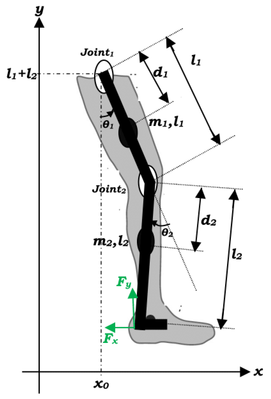
where $I_1$, $m_1$, and $l_1$ (respectively $I_2$, $m_2$, and $l_2$) are the inertia, the mass, and the length of the thigh (respectively of the shank) regarding the distance between the mass center and joint, $d_{s1}={\displaystyle \frac{l_1}{2}}$ and $d_{s2}={\displaystyle \frac{l_2}{2}}$.

The considered exoskeleton scheme is depicted in Figure 1.

It should be noted that the latter state model is established based on the Euler–Lagrange equation of a two-DOF lower-limb human exoskeleton system governed by [23]

$$M\left(\theta \right)\ddot{\theta }+C(\theta ,\dot{\theta })\dot{\theta }+G\left(\theta \right)=u+d$$

(3)

with $\theta ={[{\theta }_1,{\theta }_2]}^T$ and

$$\begin{array}{c}M\left(\theta \right)=\left(\begin{array}{cc}{M}_{11}\left(\theta \right)& M_{12}\left(\theta \right)\\ M_{21}\left(\theta \right)& M_{22}\left(\theta \right)\end{array}\right);C(\theta ,\dot{\theta })\dot{\theta }=\left(\begin{array}{c}{C}_1(\theta ,\dot{\theta })\\ C_2(\theta ,\dot{\theta })\end{array}\right)\mathrm{and}G\left(\theta \right)=\left(\begin{array}{c}{G}_1\left(\theta \right)\\ G_2\left(\theta \right)\end{array}\right)\hfill \end{array}$$

In real-life applications, lower-limb exoskeletons may be corrupted by significant unknown inputs, including unmodeled dynamics and external load torques. In practice, not all states are available for measurement due to economic constraints, such as sensor cost, and technological constraints, such as noise sensitivity or hardware integration. Moreover, external disturbances, such as unexpected torques from the environment or interaction with a human user, can degrade control accuracy if not rejected or compensated.

In this context, let us now focus on the modeling of the disturbance torque.

The reference trajectories the exoskeleton depicted in Figure 1 are provided by

$$\left\{\begin{array}{c}x=x_0+l_{1}sin\left(x_1\right)-l_{2}sin(x_2-x_1),\hfill \\ y=l_1+l_2-l_{1}cos\left(x_1\right)+l_{2}cos(x_2-x_1)\hfill \end{array}\right.$$

(4)

where $x_0$ is the initial state of the thigh joint.

The disturbance torque is provided by the following equation:

$${\tau }_d=J^{T}F=J^T\left(\begin{array}{c}{F}_x\\ F_y\end{array}\right)$$

(5)

with

$$J=\left(\begin{array}{cc}{\displaystyle \frac{\partial x}{\partial x_1}}& {\displaystyle \frac{\partial x}{\partial x_2}}\\ {\displaystyle \frac{\partial y}{\partial x_1}}& {\displaystyle \frac{\partial \mathrm{y}}{\partial x_2}}\end{array}\right)=\left(\begin{array}{cc}{l}_{1}cos\left(x_1\right)-l_{2}cos(x_2-x_1)& l_{2}cos(x_2-x_1)\\ l_{1}sin\left(x_1\right)+l_{2}sin(x_2-x_1)& +l_{2}sin(x_2-x_1)\end{array}\right)$$

$$F_x=k_{11}{x}_1(t-r_{11})+k_{21}{x}_2(t-r_{21})$$

$$F_y=k_{12}{x}_1(t-r_{12})+k_{22}{x}_2(t-r_{22})$$

Using a Taylor development, we obtain the following approximation:

$$\begin{array}{cc}\hfill F_x& \simeq k_{11}{x}_1-k_{11}{\tau }_{11}{x}_2+k_{21}{x}_3-k_{21}{\tau }_{21}{x}_4\hfill \end{array}$$

(6)

$$\begin{array}{cc}\hfill F_y& \simeq k_{12}{x}_1-k_{12}{\tau }_{12}{x}_2+k_{22}{x}_3-k_{22}{\tau }_{22}{x}_4\hfill \end{array}$$

(7)

It follows that

$$\left\{\begin{array}{c}{d}_1\simeq [l_{1}cos\left(x_1\right)-l_{2}cos(x_3-x_1)]·[k_{11}{x}_1-k_{11}{\tau }_{11}{x}_2+k_{21}{x}_3-k_{21}{\tau }_{21}{x}_4]\hfill \\ +[l_{1}sin\left(x_1\right)+l_{2}sin(x_3-x_1)]·[k_{12}{x}_1-k_{12}{\tau }_{12}{x}_2+k_{22}{x}_3-k_{22}{\tau }_{22}{x}_4]\hfill \\ d_2\simeq [l_{2}cos(x_3-x_1)]·[k_{11}{x}_1-k_{11}{\tau }_{11}{x}_2+k_{21}{x}_3-k_{21}{\tau }_{21}{x}_4]\hfill \\ +[l_{2}sin(x_3-x_1)]·[k_{12}{x}_1-k_{12}{\tau }_{12}{x}_2+k_{22}{x}_3-k_{22}{\tau }_{22}{x}_4]\hfill \end{array}\right.$$

(8)

Achieving robust control objectives in the considered exoskeleton model requires the estimation of unmeasured states (angular velocities) and the reconstruction of unknown disturbances.

In this paper, the exoskeleton system dynamics are nonlinear and subject to unknown external torques. In fact, our cascade observer-based control design is fundamentally nonlinear, following established nonlinear control theory, and no linearization of the exoskeleton dynamics is performed in our design, maintaining the full nonlinear model. Moreover, only joint angles are assumed to be measured. The control method to be designed must ensure robust tracking control objectives based on partial measurements despite the presence of disturbances.

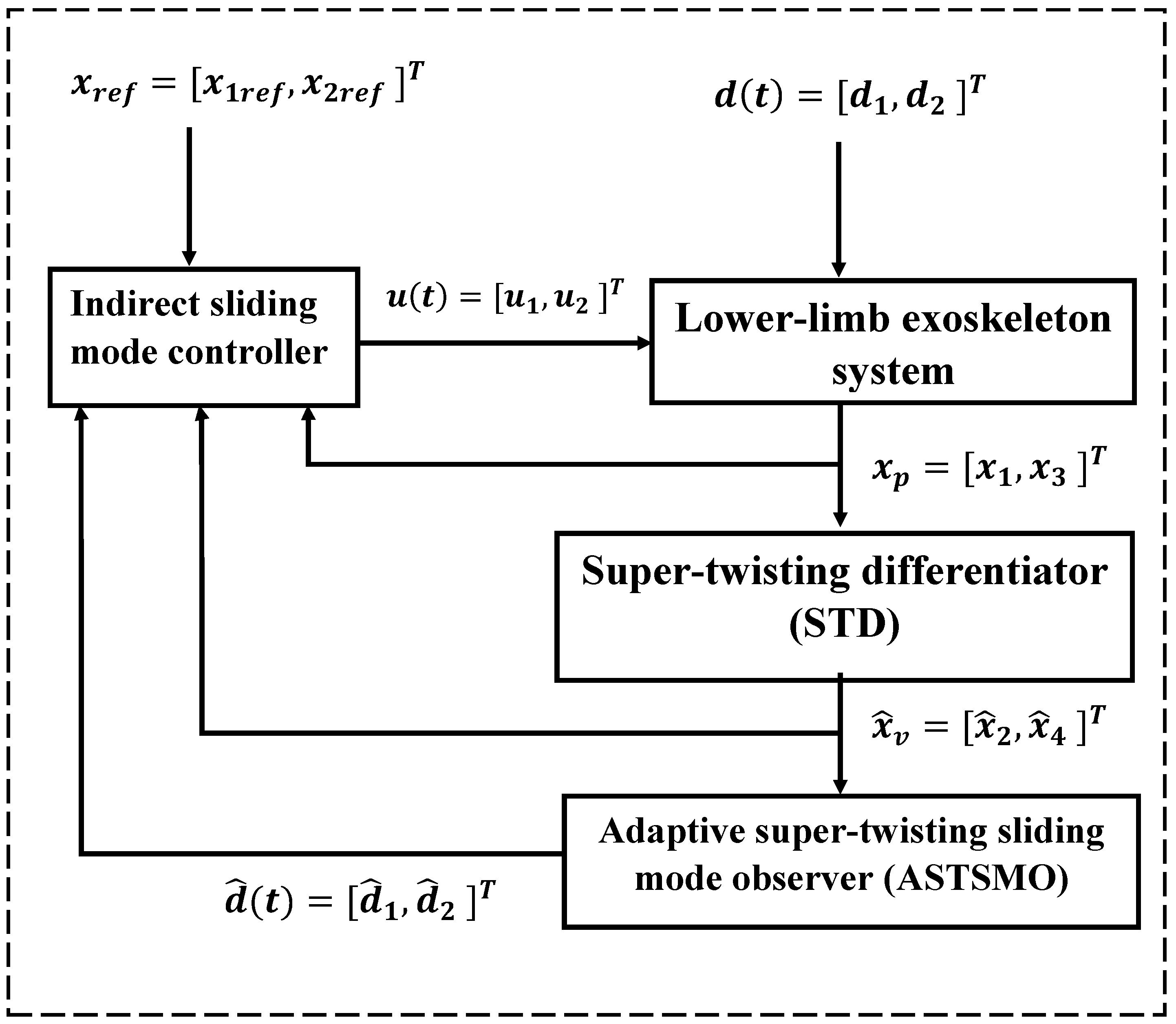
To address these challenges, a three-layer architecture is proposed in this paper. First, a super-twisting differentiator (STD) is synthesized to estimate unmeasured angular velocity states based on joint angle measurements. Second, an adaptive super-twisting sliding-mode observer (ASTSMO) is designed to estimate the external load torques, modeled as unknown disturbances based on the estimated angular velocities from the super-twisting differentiator (STD).

Then, a sliding-mode controller (SMC) uses the reconstructed disturbances and the estimated states to compute the control input: A smooth sliding surface drives the tracking error to zero. The estimated disturbance is used to compensate for the unknown input (including load torques). A saturation-based discontinuous term ensures robustness without excessive chattering. The control approach is chosen for its robustness, low chattering, and compatibility with the proposed cascade super-twisting observer.

Figure 2 represents the proposed cascaded super-twisting observer-based sliding-mode control architecture for the considered exoskeleton, including external load torque perturbations.

3. Super-Twisting Differentiator for the Estimation of Unmeasured States (Angular Velocities)

We consider the estimation of the unmeasured joint velocities $x_2={\dot{\theta }}_1$ and $x_3={\dot{\theta }}_2$, using only the available joint position measurement $x_1={\theta }_1\left(t\right)$ and $x_3={\theta }_2\left(t\right)$.

To this end, we employ a second-order super-twisting differentiator, which provides finite-time estimation of $x_2={\dot{\theta }}_1$ and $x_4={\dot{\theta }}_2$ under mild assumptions.

The second-order super-twisting differentiator that we propose is composed of two parts (a first part for the joint 1 dynamics and a second part for joint 2 dynamics).

The differentiator dynamics (for joint 1) is provided by

$$\begin{array}{ccc}\hfill {\dot{\widehat{x}}}_1\left(t\right)& =& {\widehat{x}}_2\left(t\right)+{\lambda }_1{\left|e_1\left(t\right)\right|}^{1/2}sign\left(e_1\left(t\right)\right)\hfill \end{array}$$

(9)

$$\begin{array}{ccc}\hfill {\dot{\widehat{x}}}_2\left(t\right)& =& {\rho }_{1}sign\left(e_1\left(t\right)\right)\hfill \end{array}$$

(10)

where $e_1\left(t\right)=x_1\left(t\right)-{\widehat{x}}_1\left(t\right)$ such that ${\widehat{x}}_1\left(t\right)$ is the observer estimate of $x_1\left(t\right)$, and ${\widehat{x}}_2\left(t\right)$ is the estimate of $x_2\left(t\right)={\dot{x}}_1\left(t\right)$. ${\lambda }_1>0$, ${\rho }_1>0$ are design parameters.

The differentiator dynamics (for joint 2) is provided by

$$\begin{array}{ccc}\hfill {\dot{\widehat{x}}}_3\left(t\right)& =& {\widehat{x}}_4\left(t\right)+{\lambda }_2{\left|e_3\left(t\right)\right|}^{1/2}sign\left(e_3\left(t\right)\right)\hfill \end{array}$$

(11)

$$\begin{array}{ccc}\hfill {\dot{\widehat{x}}}_4\left(t\right)& =& {\rho }_{2}sign\left(e_3\left(t\right)\right)\hfill \end{array}$$

(12)

where $e_3\left(t\right)=x_3\left(t\right)-{\widehat{x}}_3\left(t\right)$ such that ${\widehat{x}}_3\left(t\right)$ is the observer estimate of $x_3\left(t\right)$, and ${\widehat{x}}_4\left(t\right)$ is the estimate of $x_4\left(t\right)={\dot{x}}_3\left(t\right)$. ${\lambda }_2>0$, ${\rho }_2>0$ are design parameters.

First, we present the Lyapunov-based convergence proof for the joint 1 part of the sliding-mode differentiator.

Define estimation errors:

$$\begin{array}{cc}\hfill e_1\left(t\right)& =x_1\left(t\right)-{\widehat{x}}_1\left(t\right)\end{array}$$

(13)

$$\begin{array}{cc}\hfill e_2\left(t\right)& ={\dot{x}}_1\left(t\right)-{\widehat{x}}_2\left(t\right)\end{array}$$

(14)

Differentiating yields

$$\begin{array}{ccc}\hfill {\dot{e}}_1\left(t\right)& =& {\dot{x}}_1\left(t\right)-{\dot{\widehat{x}}}_1\left(t\right)=e_2\left(t\right)-{\lambda }_1{\left|e_1\left(t\right)\right|}^{1/2}\mathrm{sign}\left(e_1\left(t\right)\right)\hfill \end{array}$$

(15)

$$\begin{array}{ccc}\hfill {\dot{e}}_2\left(t\right)& =& {\ddot{x}}_1\left(t\right)-{\dot{\widehat{x}}}_2\left(t\right)={\ddot{x}}_1\left(t\right)-{\rho }_1\mathrm{sign}\left(e_1\left(t\right)\right)\hfill \end{array}$$

(16)

where $|{\ddot{x}}_1\left(t\right)|\le L$, where L is a known positive constant.

Consider the following Lyapunov function:

$$V(e_1,e_2)={\lambda }_1^2\left|e_1\right|+{\displaystyle \frac{1}{2}}{e}_2^2.$$

(17)

The time derivative of V along the trajectories is

$$\begin{array}{ccc}\hfill \dot{V}& =& {\displaystyle \frac{d}{dt}}\left[{\lambda }_1^2\left|e_1\right|+{\displaystyle \frac{1}{2}}{e}_2^2\right]\hfill \end{array}$$

(18)

$$\begin{array}{ccc}& =& {\lambda }_1^2\mathrm{sign}\left(e_1\right){\dot{e}}_1+e_2{\dot{e}}_2\hfill \end{array}$$

(19)

$$\begin{array}{ccc}& =& {\lambda }_1^2\mathrm{sign}\left(e_1\right)\left(e_2-{\lambda }_1{\left|e_1\right|}^{1/2}\mathrm{sign}\left(e_1\right)\right)+e_2\left({\ddot{x}}_1-{\rho }_1\mathrm{sign}\left(e_1\right)\right)\hfill \end{array}$$

(20)

$$\begin{array}{ccc}& =& {\lambda }_1^2\mathrm{sign}\left(e_1\right)e_2-{\lambda }_1^3|e_1{|}^{1/2}+e_2{\ddot{x}}_1-{\rho }_1\left|e_2\right|.\hfill \end{array}$$

(21)

Using $|{\ddot{x}}_1|\le L$ and the fact that $\mathrm{sign}\left(e_1\right)e_2\le \left|e_2\right|$, we have

$$\begin{array}{ccc}\hfill \dot{V}& \le & {\lambda }_1^2|e_2|-{\lambda }_1^3|e_1{|}^{1/2}+L|e_2|-{\rho }_1\left|e_2\right|\hfill \end{array}$$

(22)

$$\begin{array}{ccc}& =& -{\lambda }_1^3|e_1{|}^{1/2}-({\rho }_1-{\lambda }_1^2-L)\left|e_2\right|.\hfill \end{array}$$

(23)

If the gains are chosen such that

$$\begin{array}{cc}\hfill {\rho }_1& >{\lambda }_1^2+L,\hfill \end{array}$$

(24)

$$\begin{array}{cc}\hfill {\lambda }_1& >0,\hfill \end{array}$$

(25)

then

$$\dot{V}\le -\kappa \left(|e_1{|}^{1/2}+\left|e_2\right|\right),$$

(26)

where $\kappa =min({\lambda }_1^3,{\rho }_1-{\lambda }_1^2-L)>0$.

This proves finite-time convergence of the estimation errors to zero.

An identical proof of convergence is applied for the joint 2 part of the super-twisting differentiator for the estimation $x_4={\dot{\theta }}_2\left(t\right)$.

In fact, for joint 2, we define the estimation errors:

$$\begin{array}{cc}\hfill e_3\left(t\right)& =x_3\left(t\right)-{\widehat{x}}_3\left(t\right)\hfill \\ \hfill e_4\left(t\right)& ={\dot{e}}_3\left(t\right)={\dot{x}}_3\left(t\right)-{\widehat{x}}_4\left(t\right)=x_4\left(t\right)-{\widehat{x}}_4\left(t\right)\hfill \end{array}$$

and we consider the Lyapunov function

$$V(e_3,e_4)={\lambda }_2^2\left|e_3\right|+{\displaystyle \frac{1}{2}}{e}_4^2+{\displaystyle \frac{1}{2}}{\left({\lambda }_2{\left|e_4\right|}^{1/2}\mathrm{sign}\left(e_3\right)-e_4\right)}^2$$

(27)

Proceeding, as in the the convergence proof provided for the joint 1 part of the differentiator, and based on a similar Lyapunov analysis for the joint 2 part of the proposed super-twisting differentiator, we demonstrate the finite-time estimation of unmeasured joint velocity $x_4$ using the measured angle joint $x_3$.

Consequently, we deduce that the proposed super-twisting differentiator provides finite-time estimation of unmeasured joint velocities ($x_2$ and $x_4$) using only position measurements ($x_1$ and $x_3$).

4. Adaptive Super-Twisting Sliding-Mode Observer Design for the Estimation of Disturbances

The nonlinear dynamic model of a two-DOF robotic leg exoskeleton may be rewritten in the form

$$\dot{x}=\psi (x,u)+\zeta \left(t\right),$$

(28)

where $x={[x_1,x_2,x_3,x_4]}^T$, $u={[u_1,u_2]}^T$,

$$\psi (x,u)=\left(\begin{array}{c}{x}_2\\ f_2\left(x\right)+g_{21}\left(x\right)u_1+g_{22}\left(x\right)u_2\\ x_4\\ f_4\left(x\right)+g_{41}(x_1,x_3)u_1+g_{42}\left(x\right)u_2\end{array}\right)$$

(29)

and $\zeta ={[{\zeta }_1,{\zeta }_2]}^T$ denotes an unknown input function depending on the load torque disturbance $d={[d_1,d_2]}^T$ as follows:

$$\begin{array}{ccc}\hfill {\zeta }_1& =& g_{21}\left(x\right)d_1+g_{22}\left(x\right)d_2,\hfill \end{array}$$

(30)

$$\begin{array}{ccc}\hfill {\zeta }_2& =& g_{41}\left(x\right)d_1+g_{42}\left(x\right)d_2.\hfill \end{array}$$

(31)

We propose the following adaptive super-twisting sliding-mode observer, whose objective consists of reconstructing the state $x\left(t\right)$ and the unknown input function $\zeta \left(t\right)$ (which enables deducing the reconstruction of the load torque disturbance $d\left(t\right)$):

$$\left\{\begin{array}{c}{\dot{z}}_2=f_2(x_1,{\widehat{x}}_2,x_3,{\widehat{x}}_4)+g_{21}(x_1,x_3)u_1+g_{22}(x_1,x_3)u_2+{\gamma }_1{|{\widehat{x}}_2-z_2|}^{1/2}sign(x_2-z_2)+{\widehat{\zeta }}_1\hfill \\ {\dot{\widehat{\zeta }}}_1={\sigma }_1(x_2-z_2)\hfill \\ {\dot{z}}_4=f_4(x_1,{\widehat{x}}_2,x_3,{\widehat{x}}_4)+g_{41}(x_1,x_3)u_1+g_{42}(x_1,x_3)u_2+{\gamma }_2{|{\widehat{x}}_4-z_4|}^{1/2}sign(x_4-z_4)+{\widehat{\zeta }}_2\hfill \\ {\dot{\widehat{\zeta }}}_2={\sigma }_2(x_4-z_4)\hfill \end{array}\right.$$

(32)

where ${\widehat{x}}_2$ and ${\widehat{x}}_4$ are the respective estimates of angular velocity states $x_2$ and $x_4$ provided after a finite time from the first super-twisting differentiator described by dynamics (9) and (11).

The proposed adaptive super-twisting sliding-mode observer (32) may be written in the following compact form:

$$\left\{\begin{array}{c}{\dot{z}}_v=\varphi (x_1,{\widehat{x}}_2,x_3,{\widehat{x}}_4)+\Gamma {|x_v-z_v|}^{1/2}sign({\widehat{x}}_v-z_v)+\widehat{\zeta }\hfill \\ \dot{\widehat{\zeta }}=R({\widehat{x}}_v-z_v)\hfill \end{array}\right.$$

(33)

Define $e_v={[e_{v1},e_{v2}]}^T=x_v-z_v$: the estimation error, with ${\widehat{x}}_v={[{\widehat{x}}_2,{\widehat{x}}_4]}^T$ the finite-time estimate of $x_v={[x_2,x_4]}^T$ provided from the first super-twisting differentiator described by dynamics (9) and (11) and $z_v={[z_2,z_4]}^T$. $\Gamma =\mathrm{diag}({\gamma }_1,{\gamma }_2)$, $R=\mathrm{diag}({\sigma }_1,{\sigma }_2)$.

$$\varphi (x_1,{\widehat{x}}_2,x_3,{\widehat{x}}_4,u)=\left(\begin{array}{c}{f}_2(x_1,{\widehat{x}}_2,x_3,{\widehat{x}}_4)+g_{21}(x_1,x_3)u_1+g_{22}(x_1,x_3)u_2\\ f_4(x_1,{\widehat{x}}_2,x_3,{\widehat{x}}_4)+g_{41}(x_1,x_3)u_1+g_{42}(x_1,x_3)u_2\end{array}\right).$$

The error’s system may be written in the following form:

$$\left\{\begin{array}{c}\dot{e_v}=\varphi (x_1,x_2,x_3,x_4,u)-\varphi (x_1,{\widehat{x}}_2,x_3,{\widehat{x}}_4,u)-\Gamma {|{\widehat{x}}_v-z_v|}^{1/2}sign({\widehat{x}}_v-z_v)+\zeta -\widehat{\zeta }\hfill \\ \dot{\widehat{\zeta }}=R({\widehat{x}}_v-z_v)\hfill \end{array}\right.$$

(34)

Using the previous proof of finite-time estimation of angular velocities provided by the first super-twisting differentiator described by dynamics (9) and (11), we assume that, after a finite time $t_f$, ${\widehat{x}}_2\simeq x_2$ and ${\widehat{x}}_4\simeq x_4$, and, consequently, for $t>t_f$, we have ${\widehat{x}}_v\simeq x_v$ (hence, $e_v=x_v-z_v\simeq {\widehat{x}}_v-z_v$) and $\varphi (x_1,x_2,x_3,x_4,u)-\varphi (x_1,{\widehat{x}}_2,x_3,{\widehat{x}}_4,u)\simeq 0$.

Then, for $t>t_f$, the error’s system may be written as

$$\left\{\begin{array}{c}{\dot{e}}_v=-\Gamma {\left|e_v\right|}^{1/2}sign\left(e_v\right)+\zeta -\widehat{\zeta }\hfill \\ \dot{\widehat{\zeta }}=R{e}_v\hfill \end{array}\right.$$

(35)

We consider the Lyapunov function

$$V(e_v,\widehat{\zeta })={\displaystyle \frac{1}{2}}{e}_v^T{e}_v+{\displaystyle \frac{1}{2}}\sum _{i=1}^2{\displaystyle \frac{{({\widehat{\zeta }}_i-{\zeta }_i)}^2}{{\sigma }_i}}$$

(36)

For $t>t_f$, the time derivative of $V(e_v,\zeta )$ along the trajectories of the error’s system is provided by

$$\begin{array}{cc}\hfill \dot{V}& =e_v^T{\dot{e}}_v+\sum _{i=1}^2{\displaystyle \frac{({\widehat{\zeta }}_i-{\zeta }_i)({\dot{\widehat{\zeta }}}_i-{\dot{\zeta }}_i)}{{\sigma }_i}}\hfill \end{array}$$

(37)

$$\begin{array}{cc}\hfill & =e_v^T[\zeta -\widehat{\zeta }-\Gamma |e_v{|}^{1/2}sign\left(e_v\right)]+\sum _{i=1}^2\left[({\widehat{\zeta }}_i-{\zeta }_i)e_{vi}-{\displaystyle \frac{({\widehat{\zeta }}_i-{\zeta }_i){\dot{\zeta }}_i}{{\sigma }_i}}\right]\hfill \end{array}$$

(38)

It follows that

$$\begin{array}{ccc}\hfill \dot{V}& =& -e_v^T\Gamma {\left|e_v\right|}^{1/2}sign\left(e_v\right)+e_v^T(\zeta -\widehat{\zeta })+{(\widehat{\zeta }-\zeta )}^T{e}_v-\sum _{i=1}^2{\displaystyle \frac{({\widehat{\zeta }}_i-{\zeta }_i){\dot{\zeta }}_i}{{\sigma }_i}}\hfill \end{array}$$

(39)

Since ${(\widehat{\zeta }-\zeta )}^T{e}_v=e_v^T(\widehat{\zeta }-\zeta )=-e_v^T(\zeta -\widehat{\zeta })$, the cross terms cancel:

$$\dot{V}=-\sum _{i=1}^2{\gamma }_i{\left|e_{vi}\right|}^{3/2}-\sum _{i=1}^2{\displaystyle \frac{({\widehat{\zeta }}_i-{\zeta }_i){\dot{\zeta }}_i}{{\sigma }_i}}$$

(40)

Assuming $|{\dot{\zeta }}_i|\le {\delta }_i$, where ${\delta }_i$ are small positive design parameters introduced to guarantee finite-time convergence, with $i\in \{1,2\}$, we deduce

$$\dot{V}\le -\sum _{i=1}^2{\gamma }_i|e_{vi}{|}^{3/2}+\sum _{i=1}^2{\displaystyle \frac{{\delta }_i}{{\sigma }_i}}|{\widehat{\zeta }}_i-{\zeta }_i|.$$

(41)

Choosing appropriate positive parameters ${\gamma }_i$ and sufficiently large values of ${\sigma }_i$, we obtain a decreasing Lyapunov function $V\left(t\right)$.

Using classical results of high-order sliding-mode observer stability, we deduce that

$$e_v\left(t\right)\to 0\mathrm{and}\widehat{\zeta }\left(t\right)\to \zeta \left(t\right)\mathrm{in}\mathrm{finite}\mathrm{time}.$$

(42)

Finally, considering Equation (30), highlighting the relation between $\zeta \left(t\right)$ and $d\left(t\right)$, the load torque disturbance $d\left(t\right)$ may be estimated as follows:

$$\widehat{d}={\left[G_m(x_1,x_3)\right]}^{-1}[{\widehat{\zeta }}_1;{\widehat{\zeta }}_2];$$

(43)

where

$$G_m\left(x\right)=\left(\begin{array}{cc}{g}_{21}(x_1,x_3)& g_{22}(x_1,x_3)\\ g_{41}(x_1,x_3)& g_{42}(x_1,x_3).\end{array}\right);$$

(44)

We conclude that the proposed adaptive super-twisting sliding-mode observer ensures robust convergence of estimation errors and enables asymptotic reconstruction of unknown input vector $\zeta \left(t\right)$ as well as the load torque disturbance $d\left(t\right)$ in a two-DOF exoskeleton model.

5. Sliding-Mode Control Design

Robust tracking and disturbance rejection are crucial in robotic exoskeletons operating in uncertain environments. Sliding-mode control (SMC) is well known for its robustness, and, when combined with a robust observer such as the cascade super-twisting observer that we propose in this paper, it can ensure reliable performance with reduced chattering. In this context, we propose a sliding-mode control scheme using estimated disturbances from the designed cascade super-twisting observer.

We recall that the nonlinear dynamic model of a two-DOF robotic leg exoskeleton may be rewritten in the form (28)

$$\dot{x}=\psi (x,u)+\zeta \left(t\right),$$

(45)

where $x={[x_1,x_2,x_3,x_4]}^T$, $u={[u_1,u_2]}^T$, $\psi (x,u)$ is the nonlinear function provided in Equation (29), and $\zeta \left(t\right)$ denotes the unknown input function depending on the load torque disturbance $d\left(t\right)$, as described in Equation (30).

We define the tracking errors as follows:

$$\begin{array}{cccc}\hfill {\tilde{x}}_1& =x_1-x_1^{ref},\hfill & \hfill \hspace{0.25em}\hspace{0.25em}\hspace{0.25em}\hspace{0.25em}\hspace{0.25em}\hspace{0.25em}\hspace{0.25em}\hspace{0.25em}\hspace{0.25em}\hspace{0.25em}{s}_1& ={\dot{\tilde{x}}}_1+{\beta }_1{\tilde{x}}_1,\hfill \end{array}$$

(46)

$$\begin{array}{cccc}\hfill {\tilde{x}}_2& =x_3-x_3^{ref},\hfill & \hfill \hspace{0.25em}\hspace{0.25em}\hspace{0.25em}\hspace{0.25em}\hspace{0.25em}\hspace{0.25em}\hspace{0.25em}\hspace{0.25em}\hspace{0.25em}\hspace{0.25em}{s}_2& ={\dot{\tilde{x}}}_2+{\beta }_2{\tilde{x}}_2,\hfill \end{array}$$

(47)

and propose the control law:

$$u=u_{eq}-\widehat{d}-K\mathrm{sat}\left({\displaystyle \frac{s}{\mu }}\right)$$

where $u_{eq}=M\left(x\right)({\ddot{x}}_p^{ref}-\beta \dot{\tilde{x}})+C\left(x\right)+G\left(x\right)$, with $x_p^{ref}={[x_1^{ref},x_3^{ref}]}^T$

$$\begin{array}{c}M\left(x\right)=\left(\begin{array}{cc}{M}_{11}\left(x\right)& M_{12}\left(x\right)\\ M_{21}\left(x\right)& M_{22}\left(x\right)\end{array}\right);C\left(x\right)=\left(\begin{array}{c}{C}_1\left(x\right)\\ C_2\left(x\right)\end{array}\right)\mathrm{and}G\left(x\right)=\left(\begin{array}{c}{G}_1\left(x\right)\\ G_2\left(x\right)\end{array}\right)\hfill \end{array}$$

$\widehat{d}$ is the estimated disturbance from the adaptive super-twisting sliding-mode observer (ASTSMO). $\mathrm{sat}\left({\displaystyle \frac{s}{\mu }}\right)={\displaystyle \frac{s}{\mu }}$ if $\left|s\right|\le \mu$, else $sign\left(s\right)$.

$$\begin{array}{c}\beta =\left(\begin{array}{cc}{\beta }_1& 0\\ 0& {\beta }_2\end{array}\right);K=\left(\begin{array}{cc}{k}_1& 0\\ 0& k_2\end{array}\right)\hfill \end{array}$$

where ${\beta }_1,{\beta }_2,k_1,k_2$ are positive parameters.

It is important to note here that, in addition to the use of the estimated disturbance $\widehat{d}$ from the super-twisting sliding mode (ASTSMO) observer, the proposed sliding-mode controller also uses the estimated angular velocities ${\widehat{x}}_2$ and ${\widehat{x}}_4$ from the super-twisting differentiator (STD). However, for more simplicity and clarity, we assume that, after a finite time $t_f$, ${\widehat{x}}_2\simeq x_2$ and ${\widehat{x}}_4\simeq x_4$, referring to the demonstration of finite-time estimation of angular velocities provided by the first super-twisting differentiator described by dynamics (9) and (11).

Furthermore, note that, by using the proposed sliding-mode control (SMC) structure (compensation via estimated disturbance and smooth saturation), we avoid direct discontinuous injection compared to standard first-order sliding-mode control, which suffers from high-frequency chattering, damaging actuators, and terminal or adaptive SMCs, which often still inject discontinuities and amplify noise.

For the control input design, we assume that the matrix $M\left(x\right)$ is symmetric positive definite. The disturbance $d\left(t\right)$ is bounded and differentiable.

We consider the candidate Lyapunov function:

$$V={\displaystyle \frac{1}{2}}{s}_1^2+{\displaystyle \frac{1}{2}}{s}_2^2.$$

(48)

Differentiating V, we obtain the following result:

$$\dot{V}=s_1{\dot{s}}_1+s_2{\dot{s}}_2.$$

(49)

Exploiting the model form (3) of exoskeleton system and substituting closed-loop dynamics, for $i\in \{1,2\}$, we have

$${\dot{s}}_i=(d_i-{\widehat{d}}_i)-k_i\mathrm{sat}({\displaystyle \frac{s_i}{\mu }}).$$

(50)

Consequently, we obtain

$$\dot{V}=\sum _{i=1}^2{s}_i\left[(d_i-{\widehat{d}}_i)-k_i\mathrm{sat}\left({\displaystyle \frac{s_i}{\mu }}\right)\right]$$

(51)

Let ${\tilde{d}}_i=d_i-{\widehat{d}}_i$, with $|{\tilde{d}}_i|\le D_i$, and assume $k_i>D_i$.

First, we consider the case where $|s_i|\le \mu$:

$$\mathrm{sat}\left({\displaystyle \frac{s_i}{\mu }}\right)={\displaystyle \frac{s_i}{\mu }}$$

(52)

$$s_i\left[{\tilde{d}}_i-k_i{\displaystyle \frac{s_i}{\mu }}\right]=s_i{\tilde{d}}_i-{\displaystyle \frac{k_i}{\mu }}{s}_i^2.$$

(53)

Using $s_i{\tilde{d}}_i\le \left|s_i\right|D_i\le {\delta }_i{s}_i^2+{\displaystyle \frac{D_i^2}{4{\delta }_i}}$ for any ${\delta }_i>0$:

$$s_i{\tilde{d}}_i-{\displaystyle \frac{k_i}{\mu }}{s}_i^2\le -\left({\displaystyle \frac{k_i}{\mu }}-{\delta }_i\right)s_i^2+{\displaystyle \frac{D_i^2}{4{\delta }_i}}$$

Choose ${\delta }_i={\displaystyle \frac{k_i}{2\mu }}$, so

$$s_i{\tilde{d}}_i-{\displaystyle \frac{k_i}{\mu }}{s}_i^2\le -{\displaystyle \frac{k_i}{2\mu }}{s}_i^2+{\displaystyle \frac{D_i^2\mu }{2k_i}}$$

(54)

Now, we consider the case where $|s_i|>\mu$:

$$\mathrm{sat}\left({\displaystyle \frac{s_i}{\mu }}\right)=sign\left(s_i\right)$$

(55)

$$s_i\left[{\tilde{d}}_i-k_{i}sign\left(s_i\right)\right]=s_i{\tilde{d}}_i-k_i\left|s_i\right|.$$

(56)

Since $k_i>D_i$:

$$s_i{\tilde{d}}_i-k_i|s_i|\le |s_i|D_i-k_i|s_i|=-(k_i-D_i)\left|s_i\right|<0$$

(57)

In summary, in the region $|s_i|\le \mu$ for both i:

$$\dot{V}\le -{\displaystyle \frac{k_1}{2\mu }}{s}_1^2-{\displaystyle \frac{k_2}{2\mu }}{s}_2^2+{\displaystyle \frac{D_1^2\mu }{2k_1}}+{\displaystyle \frac{D_2^2\mu }{2k_2}}$$

(58)

$$\dot{V}\le =-\alpha V+\beta$$

(59)

where

$$\alpha =min\left({\displaystyle \frac{k_1}{\mu }},{\displaystyle \frac{k_2}{\mu }}\right)={\displaystyle \frac{min(k_1,k_2)}{\mu }},\beta ={\displaystyle \frac{D_1^2\mu }{2k_1}}+{\displaystyle \frac{D_2^2\mu }{2k_2}}$$

Outside this region, $\dot{V}\le 0$.

Consequently, we conclude that all trajectories converge to the set $V\le {\displaystyle \frac{\beta }{\alpha }}$; i.e., the system is uniformly ultimately bounded:

$$\underset{t\to \infty }{lim}\left|s_i\left(t\right)\right|\le \sqrt{{\displaystyle \frac{2\beta }{\alpha }}}$$

(60)

If $d_i=0$, then $s_i\to 0$ exponentially.

Note that the sliding surfaces are chosen as $S_i=\dot{{\tilde{x}}_i}+{\beta }_i{\tilde{x}}_i$, where ${\beta }_i$ sets the convergence speed. Gains $k_i$ are selected such that $k_i$>$D_i$, where $D_i$ is the estimated upper bound of disturbances. The boundary layer width $\mu$ is tuned empirically to balance precision and chattering suppression (see also chattering analysis in Section 6).

6. Numerical Simulations

Numerical simulations are carried out using Matlab/Simulink software by applying the cascade-adaptive super-twisting observer-based output-feedback sliding-mode control to the dynamic model of the two-DOF exoskeleton described by Equation (1), with nominal parameters provided in

Table 1. Parameters of the two-DOF lower-limb exoskeleton system.

Parameter	Description	Value
$m_1$	Thigh segment mass	3.0 kg
$m_2$	Shank segment mass	2.0 kg
$l_1$	Thigh segment length	0.5 m
$l_2$	Shank segment length	0.4 m
$d_1=l_1/2$	Distance between mass center of the thigh segment and joint	0.25 m
$d_2=l_1/2$	Distance between mass center of the shank segment and joint	0.2 m
$I_1$	Inertia of the thigh segment	$0.05\mathrm{kg}·{\mathrm{m}}^2$
$I_2$	Inertia of the shank segment	$0.02\mathrm{kg}·{\mathrm{m}}^2$
$k_{11}=k_{12}$	Stiffness-like coefficients	0.1 N/rad
$k_{21}=k_{22}$	Stiffness-like coefficients	0.2 N/rad

.

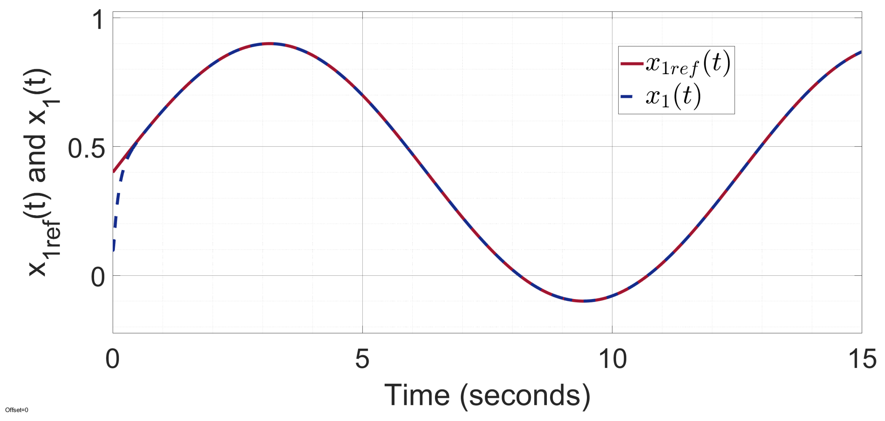
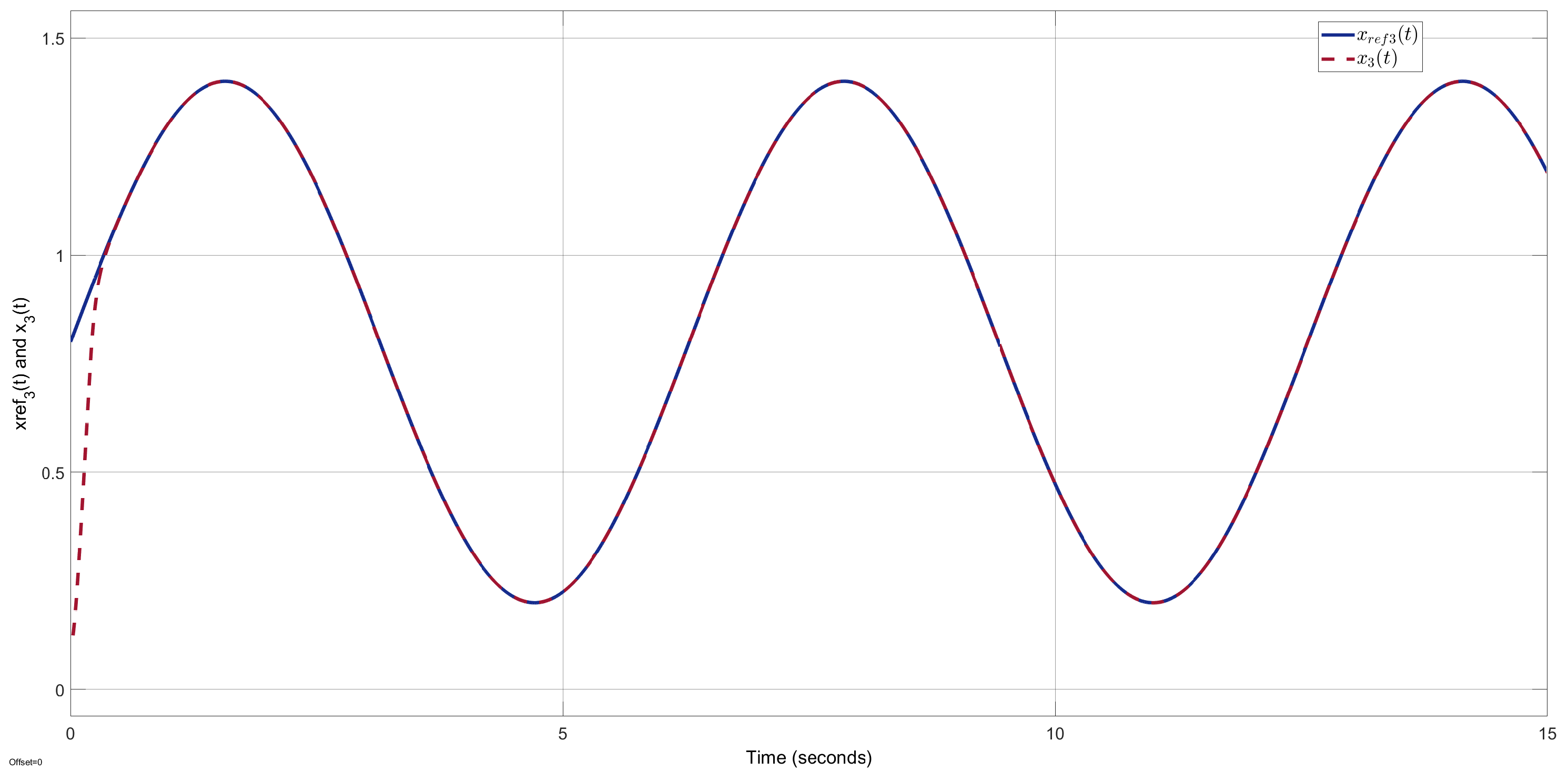
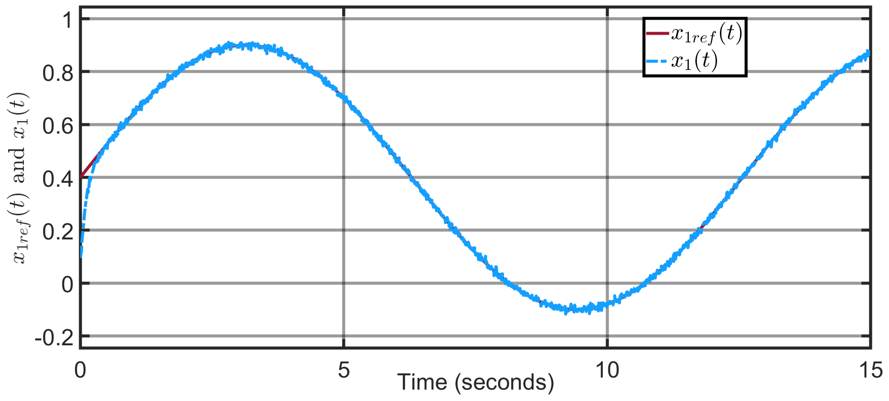
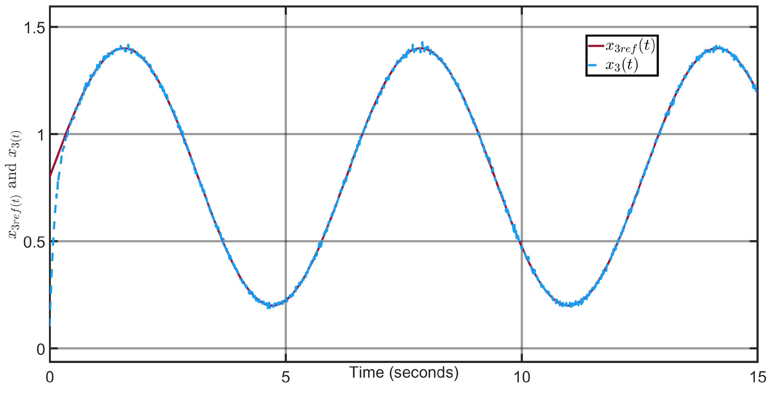
Reference trajectories are defined as $x_1^{\mathrm{ref}}=0.5sin\left(0.4t\right)+0.4$ and $x_3^{\mathrm{ref}}=0.6sin\left(0.7t\right)+0.8.$ The initial conditions for the two-link human–exoskeleton system are set as $x={\left[\begin{array}{c}0.100.10\end{array}\right]}^T.$

The super-twisting differentiator parameters are provided as follows: ${\lambda }_1=40$, ${\lambda }_2=40$, ${\rho }_1=300$, and ${\rho }_2=300$. The initial conditions for the super-twisting differentiator are set as $\widehat{x}={\left[\begin{array}{c}0.20.50.50.5\end{array}\right]}^T.$ Initial values of the super-twisting differentiator are chosen close to zero to avoid bias and ensure finite-time convergence. The adaptive super-twisting sliding-mode observer parameters are provided as follows: ${\gamma }_1=40$, ${\gamma }_2=40$, ${\sigma }_1=300$, and ${\sigma }_2=300$. The initial conditions for the adaptive super-twisting sliding-mode observer are set as $\widehat{x}={\left[\begin{array}{c}0.20.50.50.5\end{array}\right]}^T.$ The sliding-mode controller parameters are provided as follows: ${\beta }_1=10$, ${\beta }_2=10$, $k_1=10$, $k_2=10$, and $\mu =0.01$.

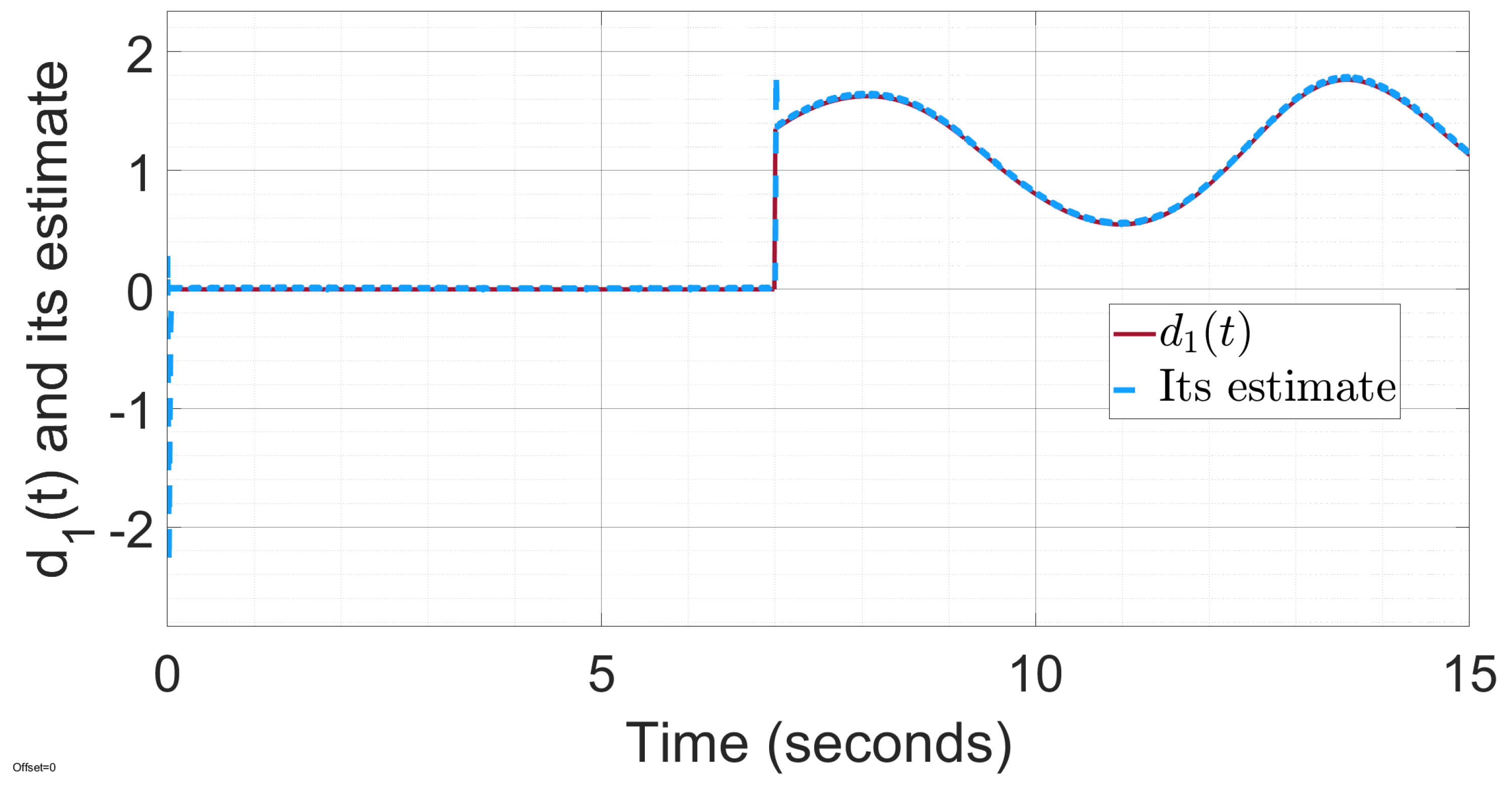
We assume that the exoskeleton system is corrupted by perturbations of two load torques $d_1\left(t\right)$ and $d_2\left(t\right)$ at time $t=7$ s.

Simulations were conducted with a sampling rate of 1 kHz (sampling time $T_s=1$ ms) following typical exoskeleton control requirements [21].

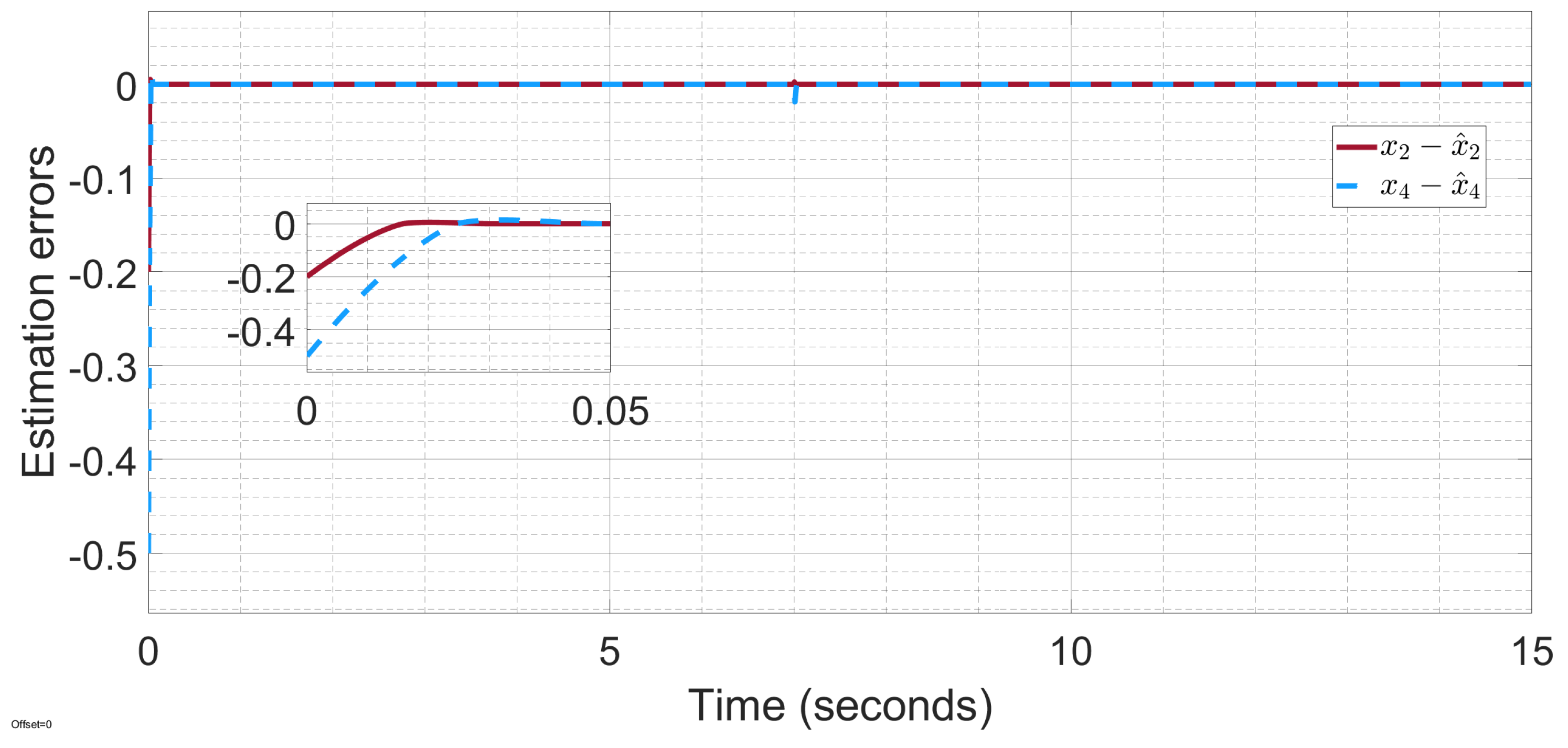
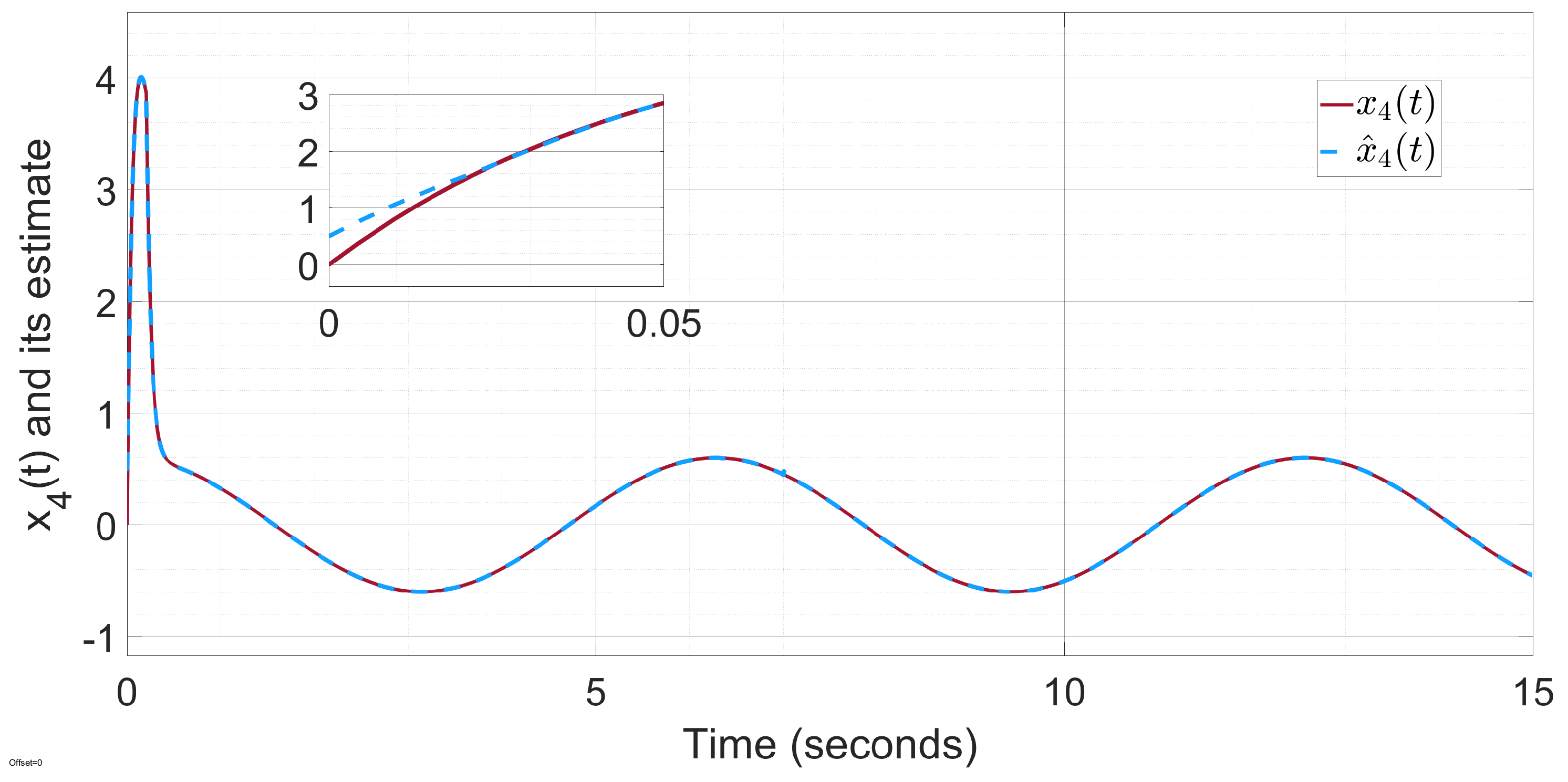
Figure 3 illustrates that the estimation errors of the angular velocity states converge to zero when time goes to infinity. Figure 4 and Figure 5 demonstrate that the unmeasured states $x_2={\dot{\theta }}_1$ and $x_4={\dot{\theta }}_2$ are well reconstructed by the proposed super-twisting differentiator.

Figure 6 and Figure 7 illustrate that the torque disturbances $d_1\left(t\right)$ and $d_2\left(t\right)$ are well reconstructed by the proposed adaptive super-twisting sliding-mode observer (ASTSMO).

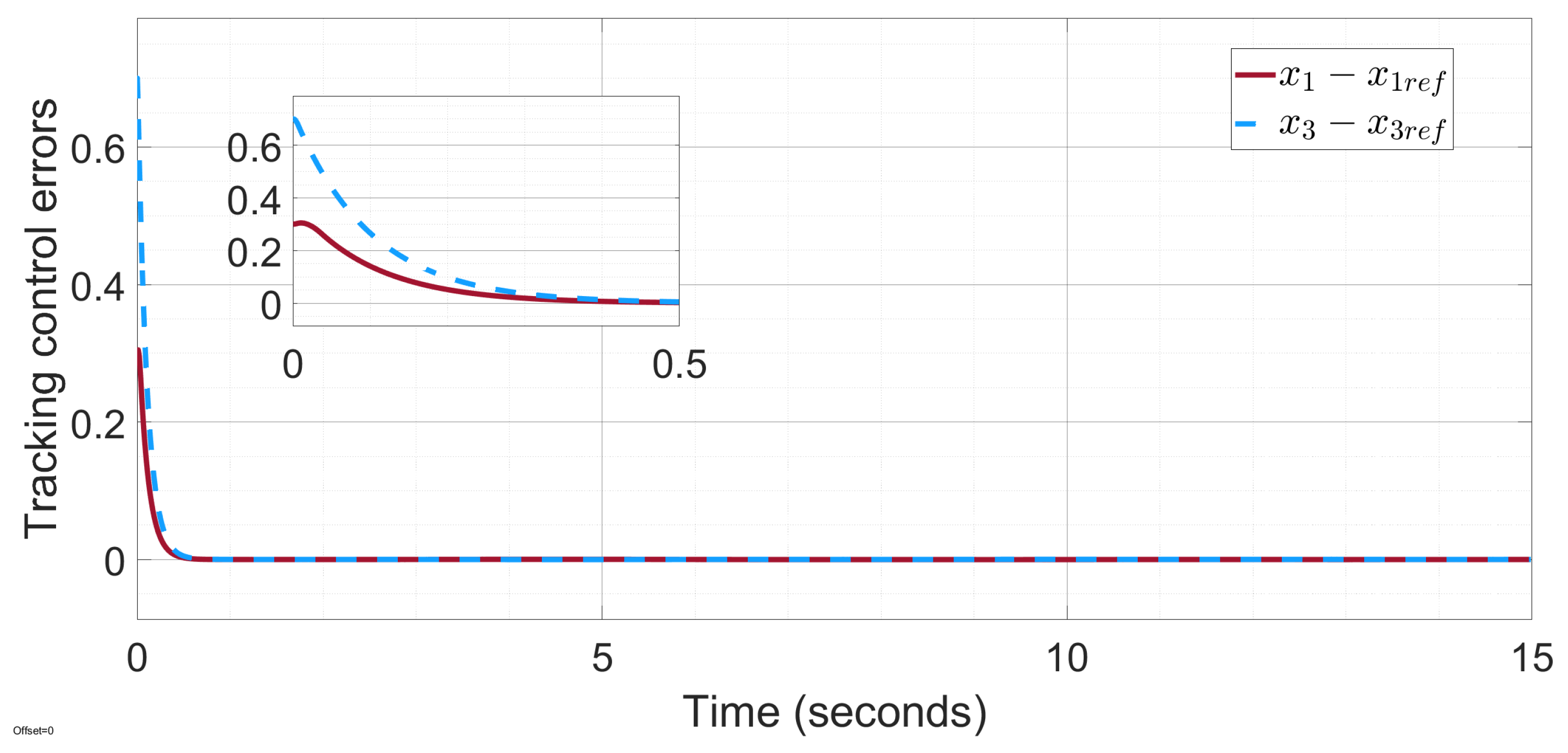
Figure 8 depicts that the tracking errors of the joint angle states converge to zero when time goes to infinity. Figure 9 and Figure 10 illustrate that the output states $x_1={\theta }_1$ and $x_2={\theta }_2$ perfectly follow the reference trajectories $x_1^{ref}$ and $x_2^{ref}$. We deduce that the proposed super-twisting observer-based sliding-mode control scheme guarantees a very satisfactory reference tracking performance despite the presence of external load torque disturbances. Indeed, the effect of latter disturbances is perfectly compensated and canceled thanks to the use of their estimates provided by the proposed adaptive super-twisting sliding-mode observer (ASTSMO).

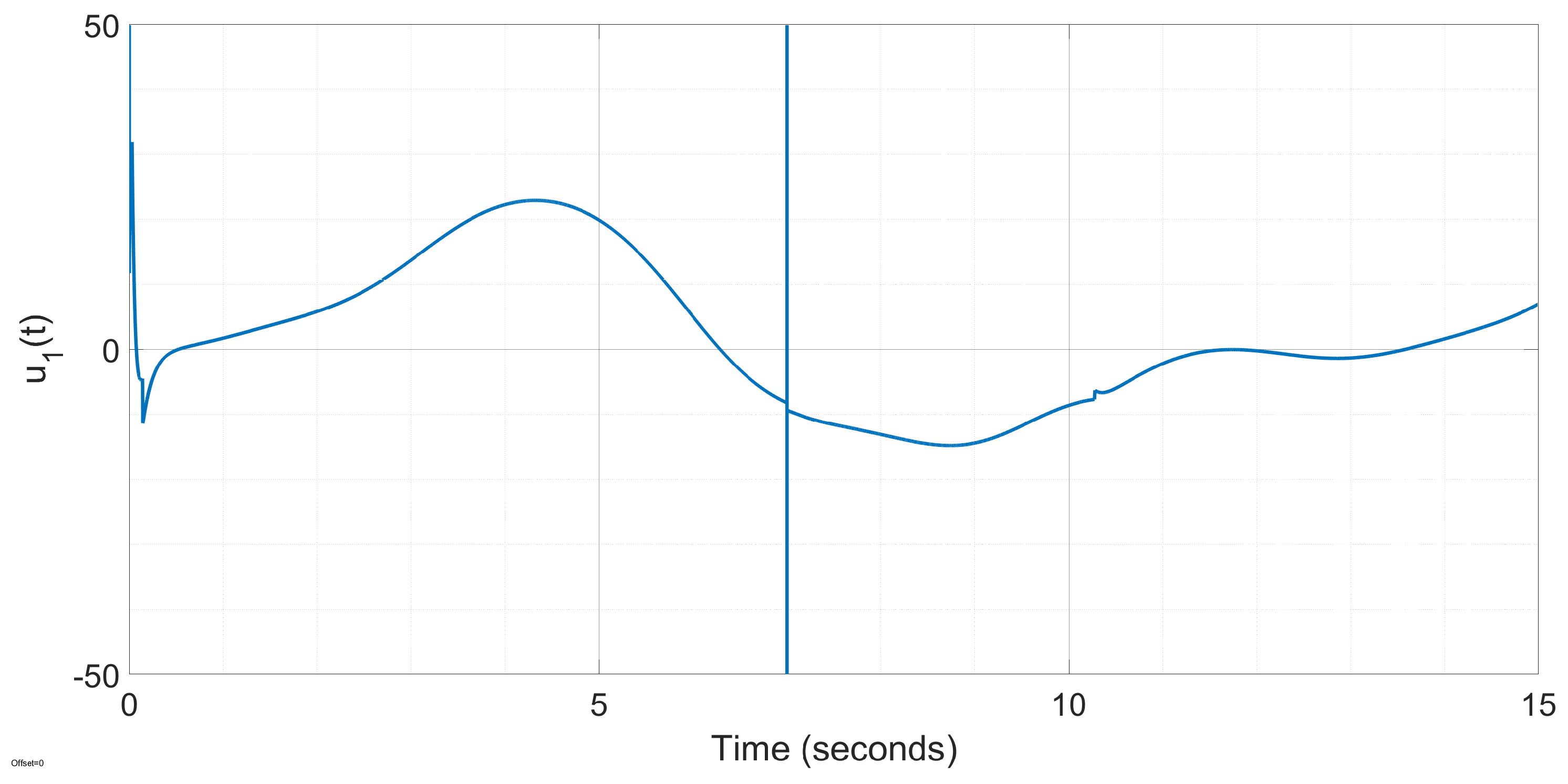
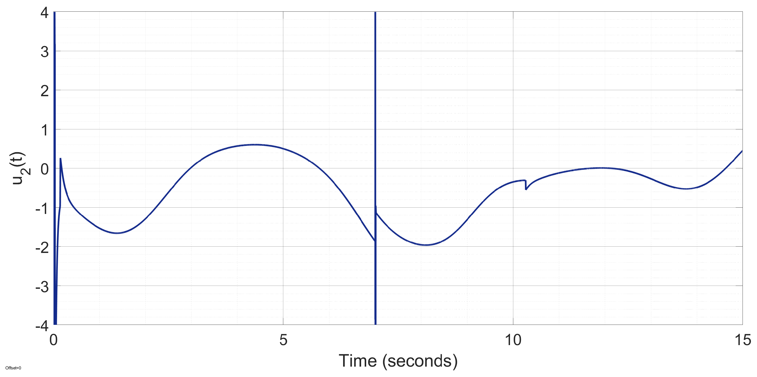
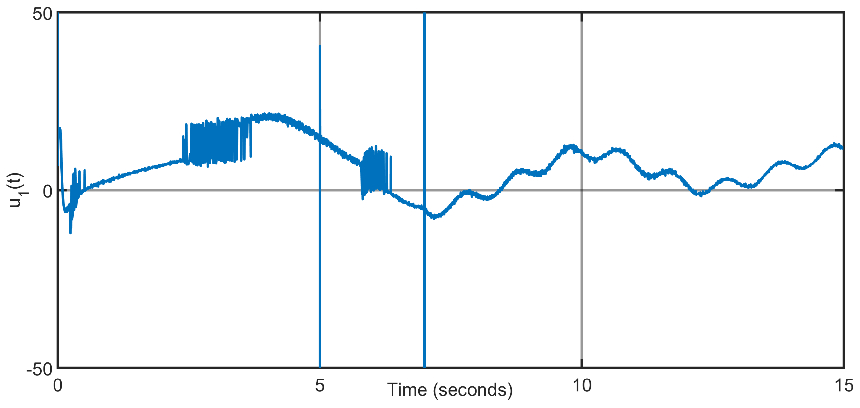
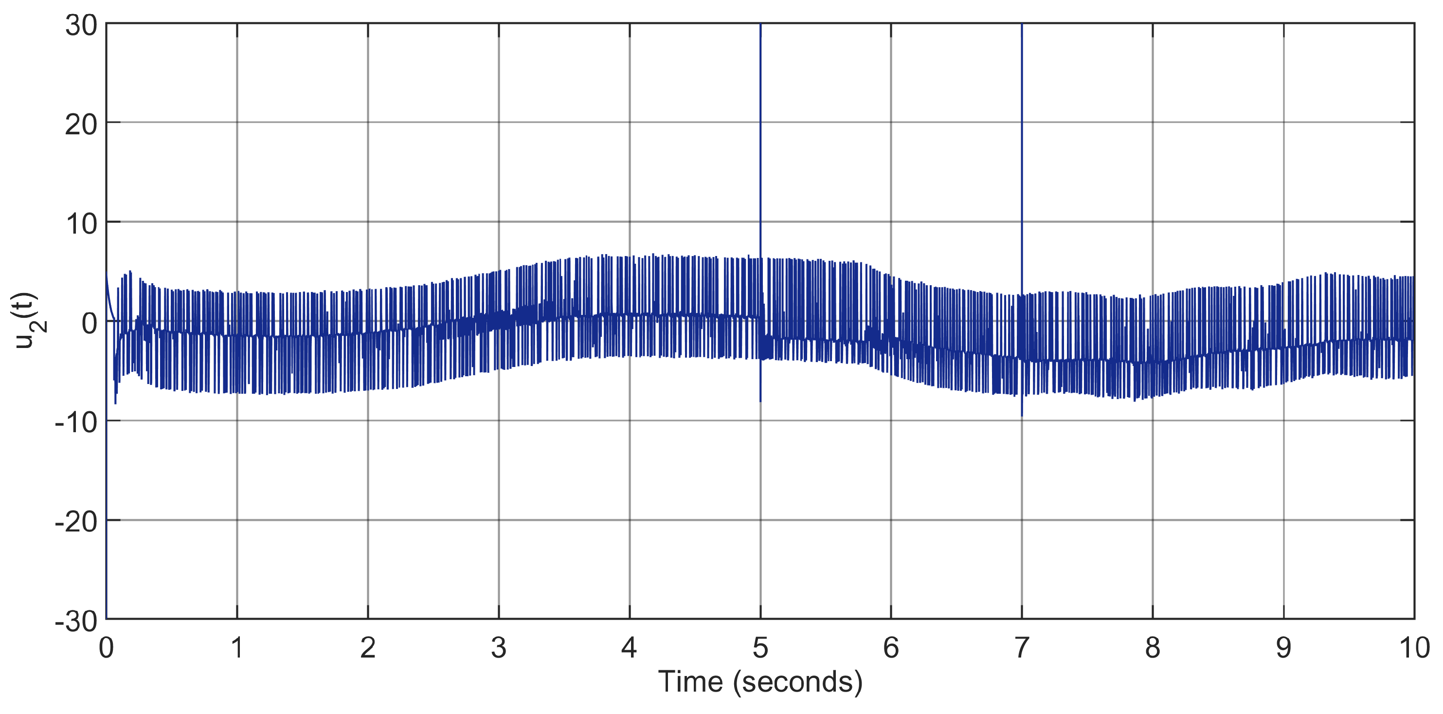
The control input torques, depicted in Figure 11 and Figure 12, exhibit greater adaptability to disturbance variations to preserve the tracking control performance.

6.1. Simulation Analysis Under Various Disturbances and Noise Effects

For more comprehensive analysis and richer testing, we have carried out additional new simulation scenarios following best practices in robust control evaluation.

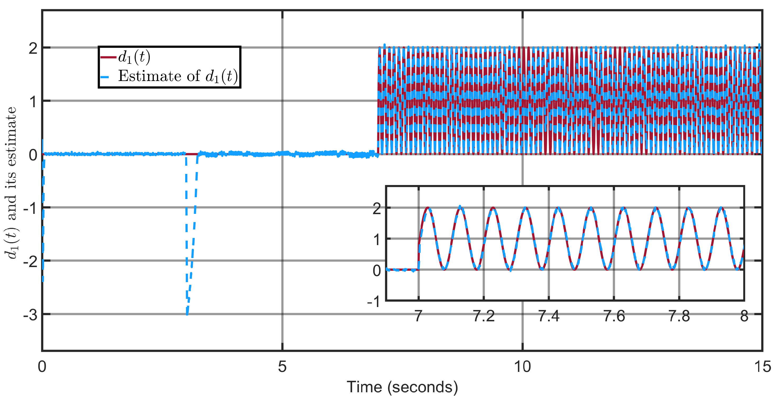
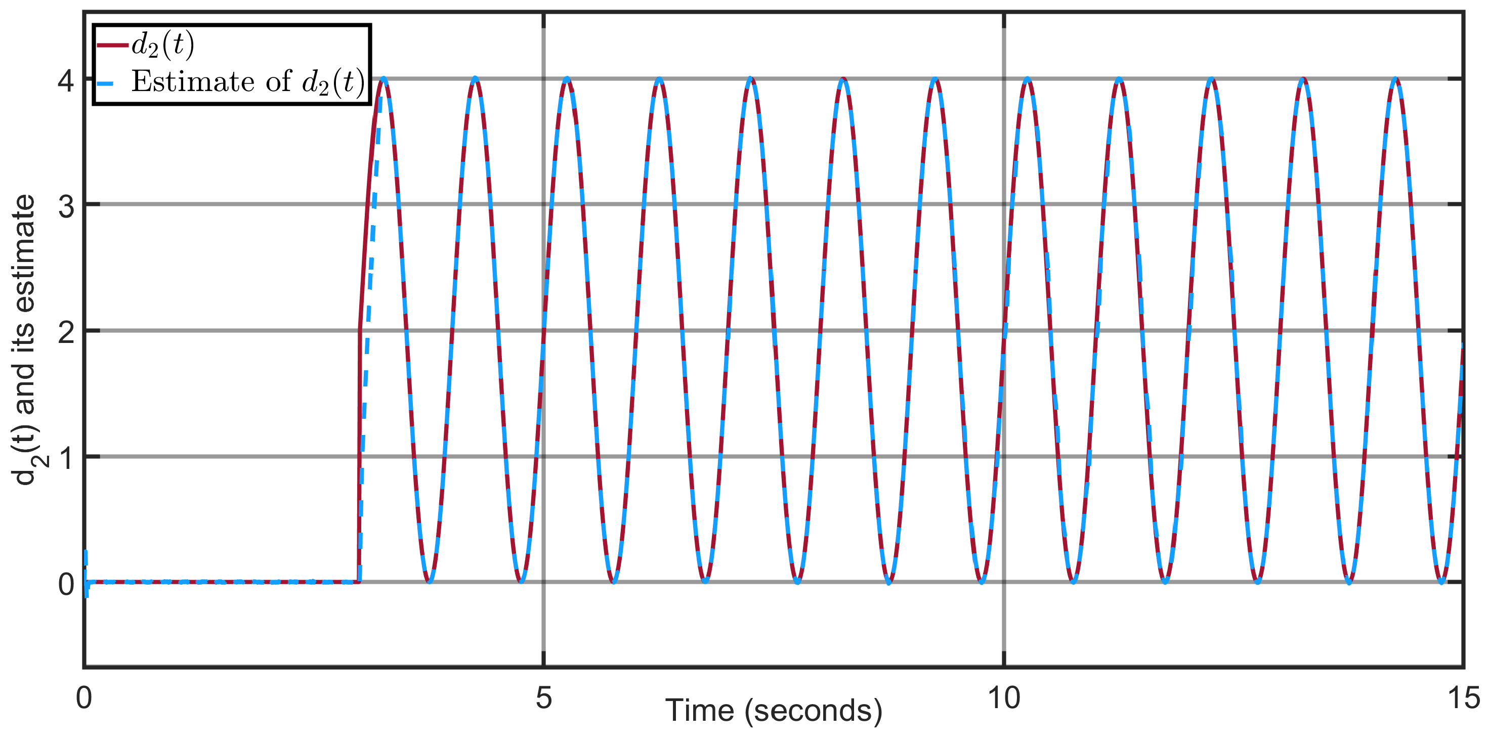
Firstly, we test the robustness of our proposed observer-based control scheme in the case where the exoskeleton system is corrupted by two sinusoidal disturbances of different frequencies and amplitudes: the disturbance $d_1\left(t\right)=2sin\left(2\pi t\right)+1$ occurring at the instant $t=7$ s and $d_2\left(t\right)=4sin\left(2\pi 10t\right)+2$ occurring at the instant $t=3$ s. Figure 13 and Figure 14 illustrate the ability of the proposed cascade observer (STD+ASTSMO) to reconstruct time-varying disturbances of different frequencies and amplitudes with very good precision.

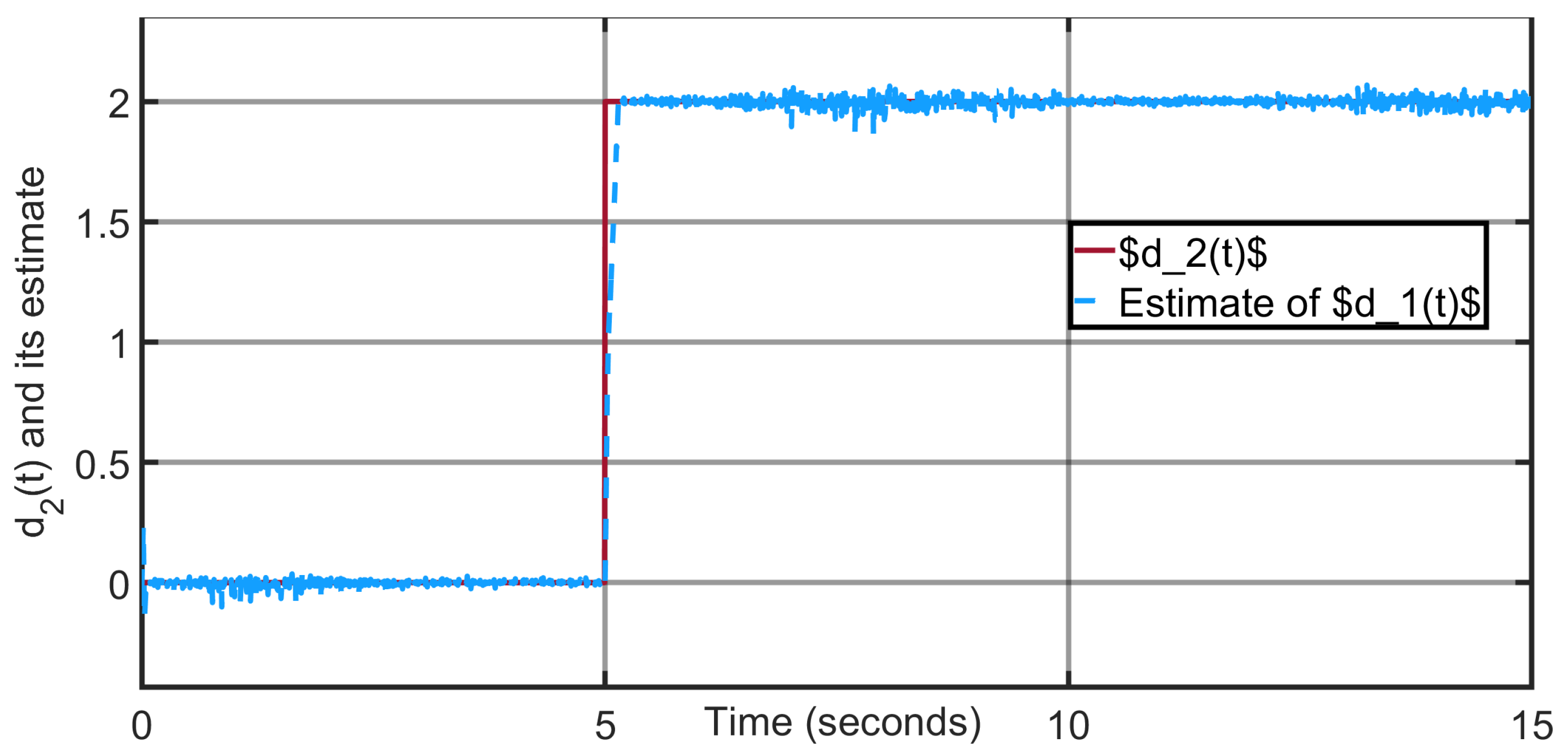
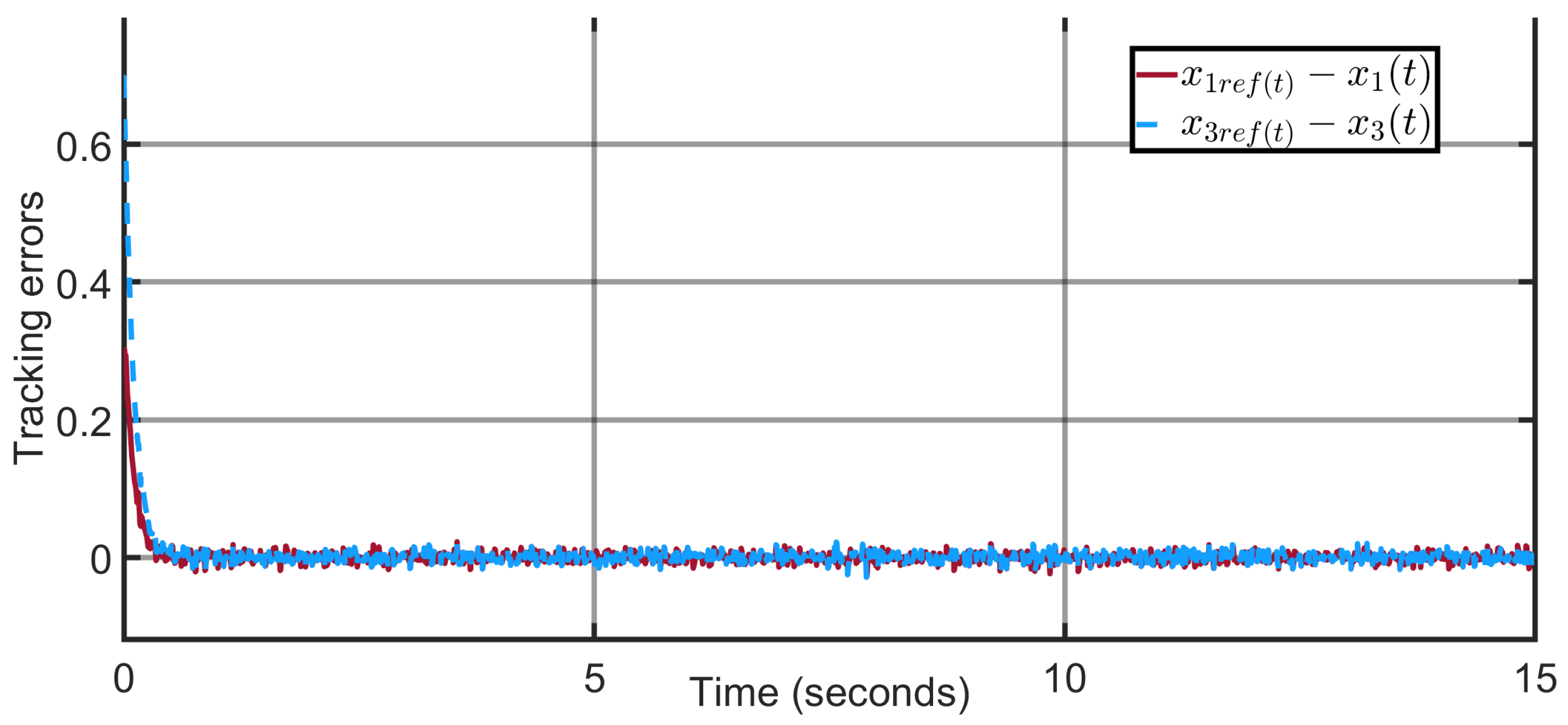
Moreover, to emulate sensor noise, an additive Gaussian noise of a power equal to ${10}^{-6}$ was added to the measured joint angles. The estimates of disturbances (Figure 15 and Figure 16), the tracking errors (Figure 17), the joint trajectories (Figure 18 and Figure 19), and the control input signals (Figure 20 and Figure 21) show that the proposed cascade observer-based sliding-mode controller maintains good performance in terms of disturbance estimation and tracking accuracy despite the presence of Gaussian noise.

6.2. Simulation Analysis Under Various Loads

In practical rehabilitation scenarios, the effective load applied to an exoskeleton joint is not strictly constant but may change due to several factors, such as the patient carrying an additional object, variations in muscle activation, or sudden shifts in limb dynamics.

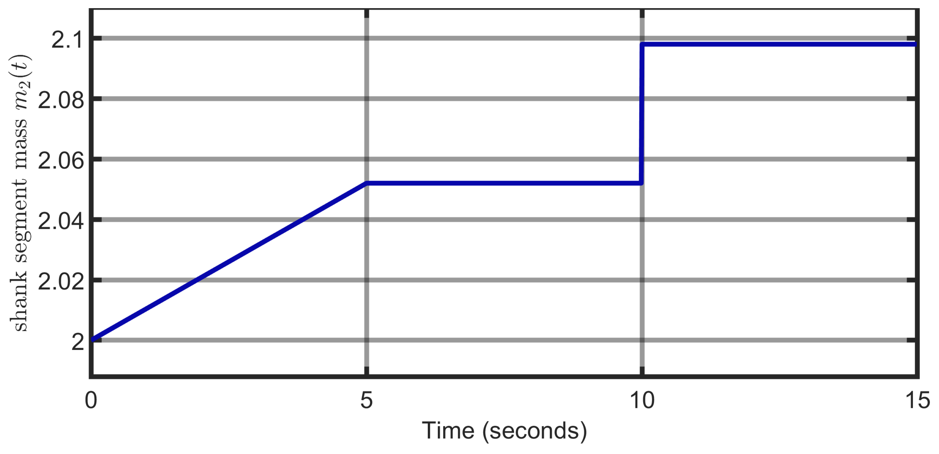
To further evaluate robustness, a disturbance scenario involving both progressive and sudden payload changes was simulated. Specifically, an additional mass of 0.1 kg was applied to the mass of shank segment $m_2$, which gradually increased in the time interval $[0,5]$ s (progressive change), followed by sudden change at time 10 s (see Figure 22).

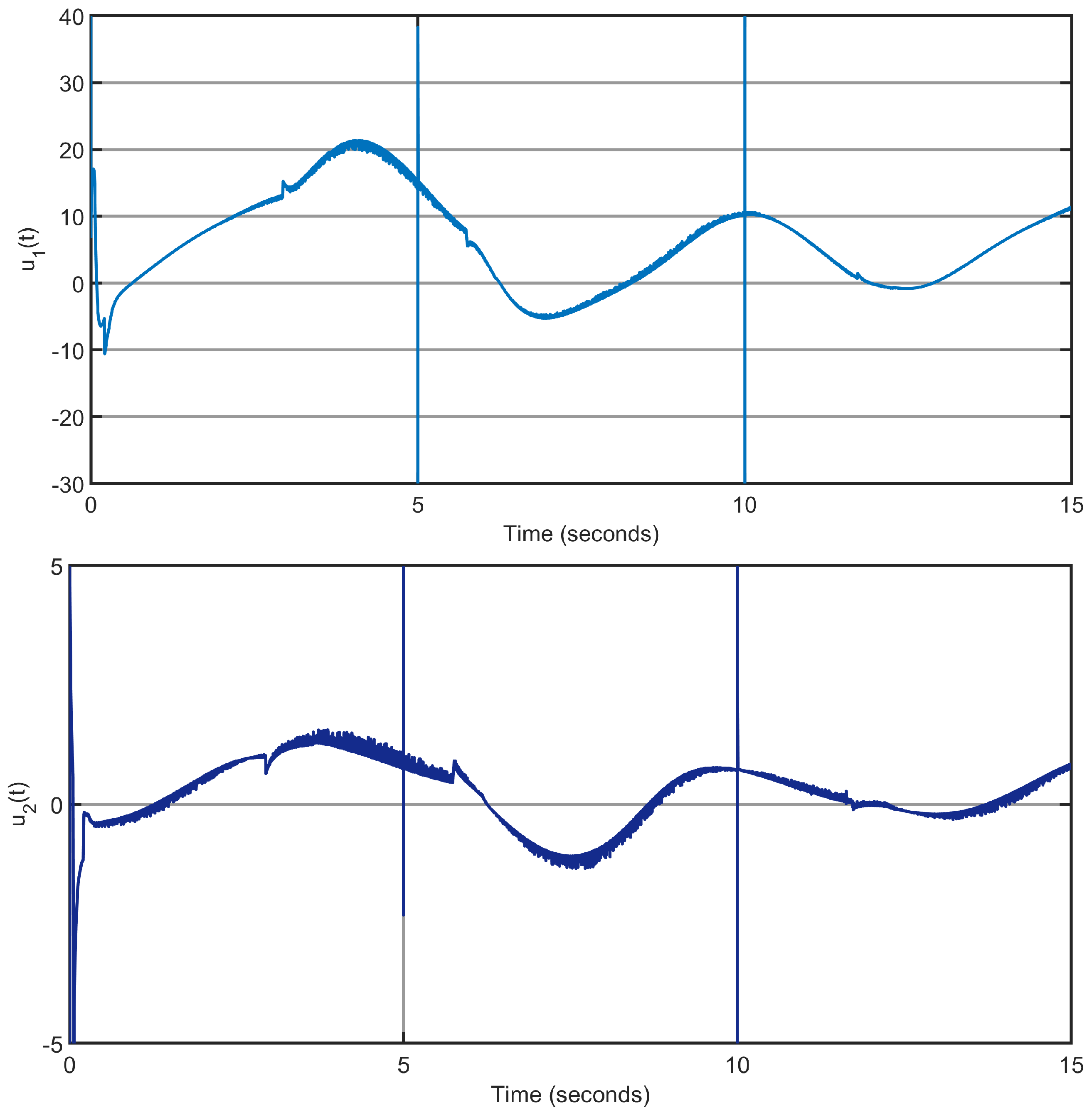
Simulation results are depicted in Figure 23 and Figure 24. The results confirm that the proposed controller maintains accurate trajectory tracking and stable state estimation under these conditions, thereby demonstrating its capability to handle both instantaneous and gradual variations in load without compromising system stability.

6.3. Sampling Rate Sensitivity Analysis

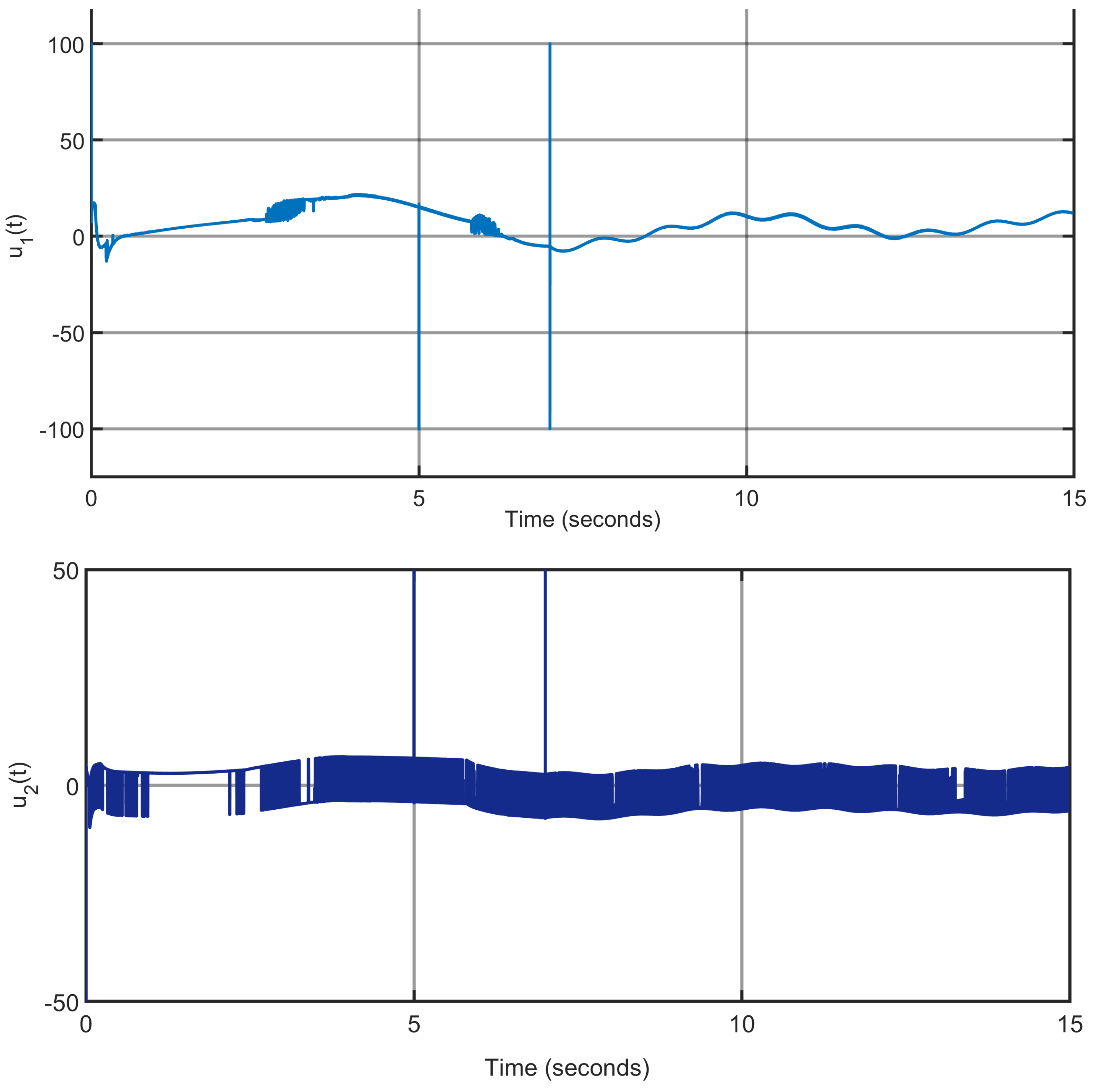
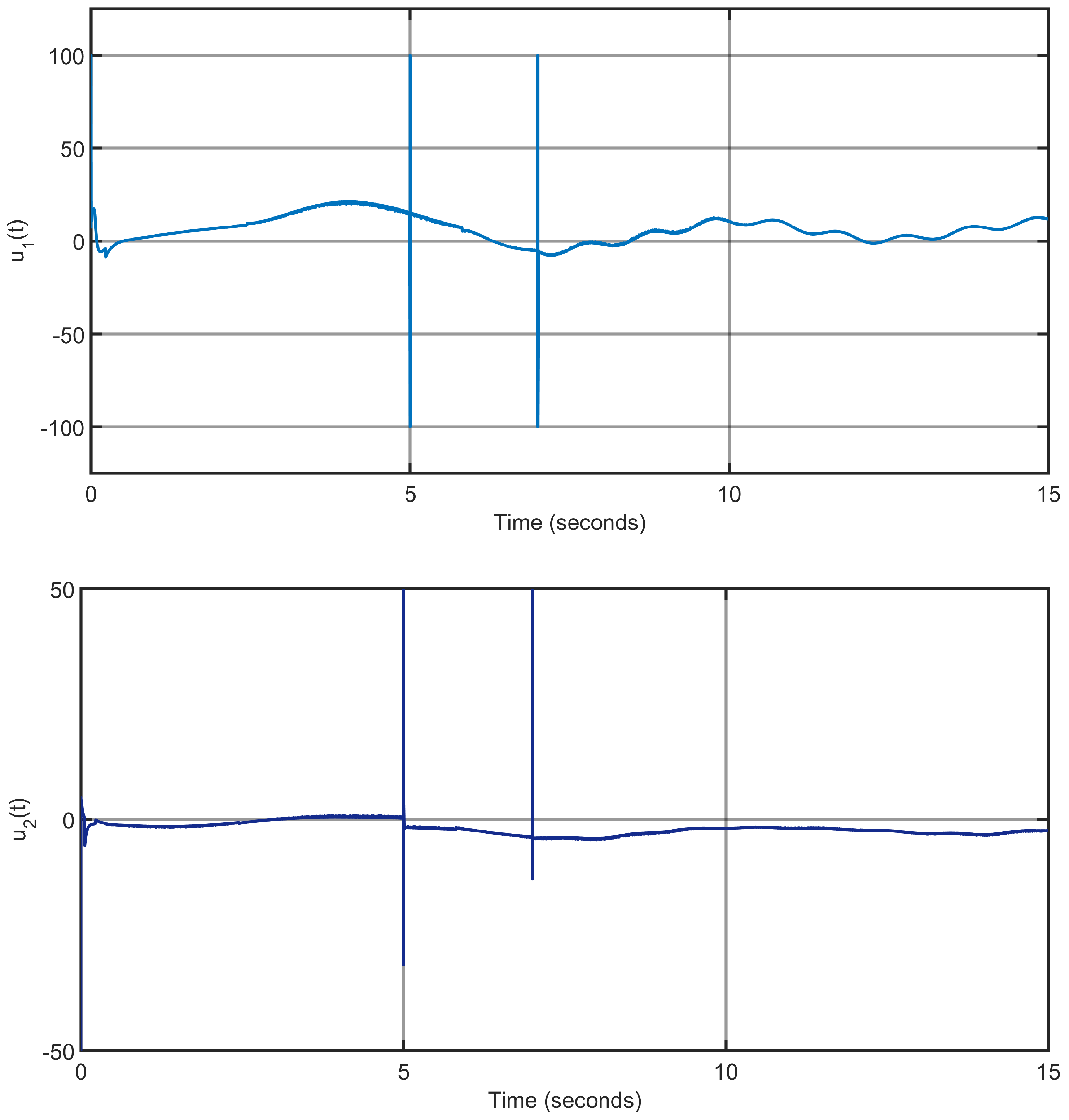
Until this stage, simulations have been realized with a sampling rate equal to 1 Khz ($T_s=1$ ms). In order to analyze the sampling rate sensitivity, we have realized a new set of simulations by showing the control torque input signals $u_1\left(t\right)$ and $u_2\left(t\right)$ for $F_s=10$ Khz ($T_s=0.1$ ms) and $F_s=100$ Hz ($T_s=10$ ms). We deduce from the obtained Figure 25 and Figure 26 that control input signals have better performance and are updated faster with the higher sampling rate ($F_s=10$ Khz) compared to the case of lower sampling rate ($F_s=100$ Hz), where we note a slight degradation in the curves of control torque input signal, which becomes less responsive.

6.4. Numerical Simulation and Quantitative Chattering Analysis

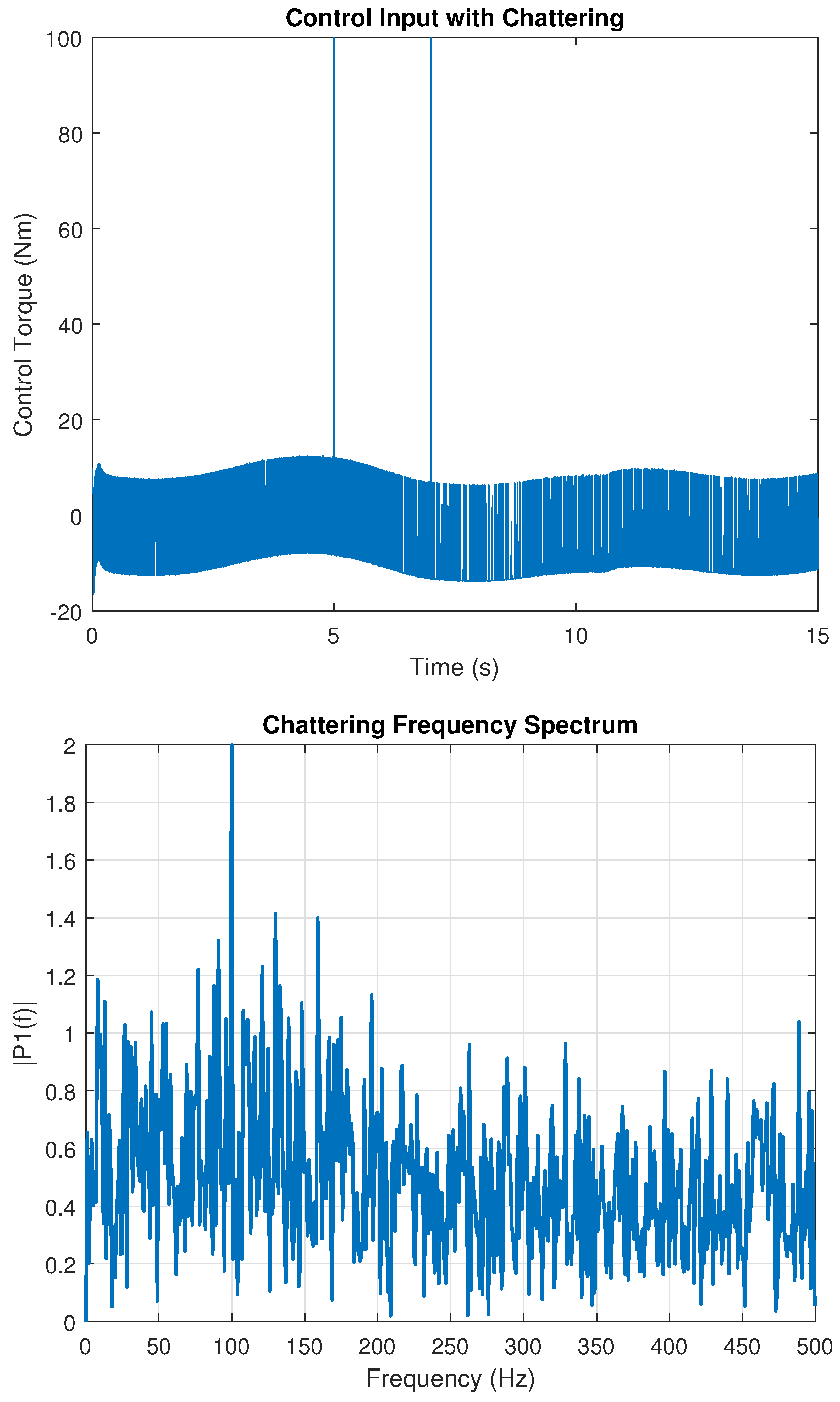
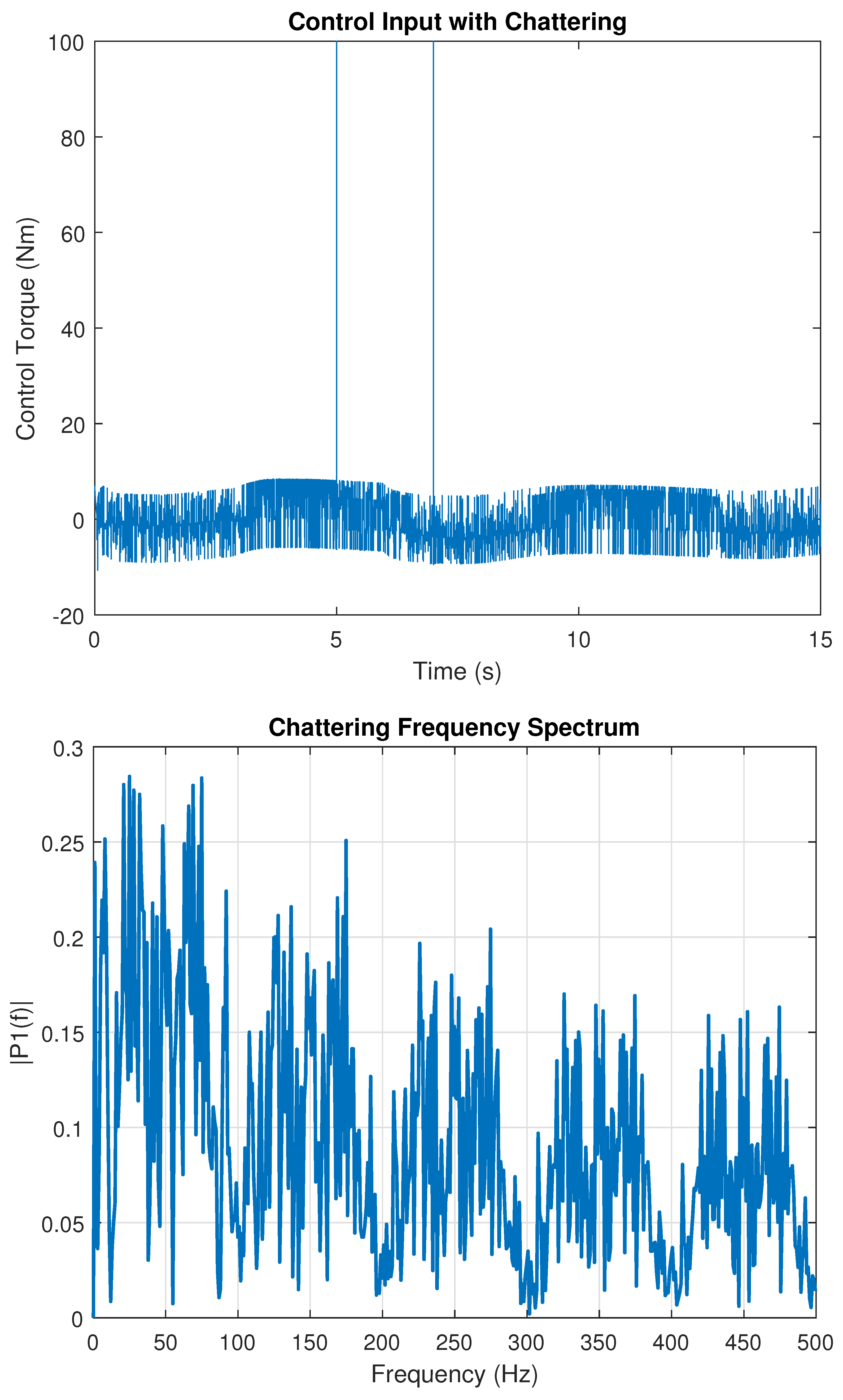
It is well known that the chattering phenomenon is the primary limitation of a sliding-mode control system that requires thorough analysis. To that end, we have developed a numerical simulation analysis of chattering in our proposed control system by showing the input torque (control signal $u_2\left(t\right)$) as well as its high-frequency content under Gaussian measurement noise of a power equal to ${10}^{-5}$ and step/sinusoidal disturbances.

To quantify the severity of chattering, we computed the $RM{S}_{HF}$ (root mean square of the high-frequency component of the control torque). We compute also the dominant high frequency (dominant HF), which represents the main frequency component of the high-frequency part of the control input (after Fast Fourier Transform (FFT)).

Three tuning configurations (three simulation experiences) were tested:

-

Experience 1 (control parameters $k_1=k_2=10$, and $\mu =0.01$): The steady-state metrics (window [2 s –3 s]) are as follows: max total torque = 12.05 Nm, $RM{S}_{HF}=8.13$ Nm, and dominant HF 118 Hz.

-

Experience 2 (control parameters $k_1=k_2=10$, and $\mu =0.001$): The steady-state metrics (window [2 s –3 s]) are as follows: max total torque = 12.05 Nm, $RM{S}_{HF}=8.31$ Nm, and dominant HF 100 Hz.

-

Experience 3 (control parameters $k_1=4,k_2=7$, and $\mu =0.05$): The steady-state metrics (window [2 s –3 s]) are as follows: max total torque = 8.54 Nm, $RM{S}_{HF}=1.51$ Nm, and dominant HF 65.9 Hz.

These results show that increasing the boundary layer $\mu$ and reducing the discontinuous gains substantially reduces the high-frequency content injected by the controller: Experience 3 reduces the HF $RM{S}_{HF}$ by $78\%$ compared with Experiences 1 and 2 while also lowering the overall commanded torque.

In Figure 27, Figure 28 and Figure 29, we show the control input $u_2\left(t\right)$ with chattering and the corresponding chattering frequency spectrum for each simulation experience and corresponding tuning configuration.

These results show that increasing the boundary layer $\mu$ (smoothing the discontinuous action) and reducing the discontinuous gains $k_1$ and $k_2$ (until a satisfactory trade-off between tracking transient and high-frequency content is obtained) substantially reduces the high-frequency content injected by the controller. A mild output filter may be also applied if necessary.

6.5. Comparative Study Between the Proposed Cascade-Adaptive Super-Twisting Sliding-Mode Observer (ASTSMO) and Standard Extended Kalman Filter (EKF)

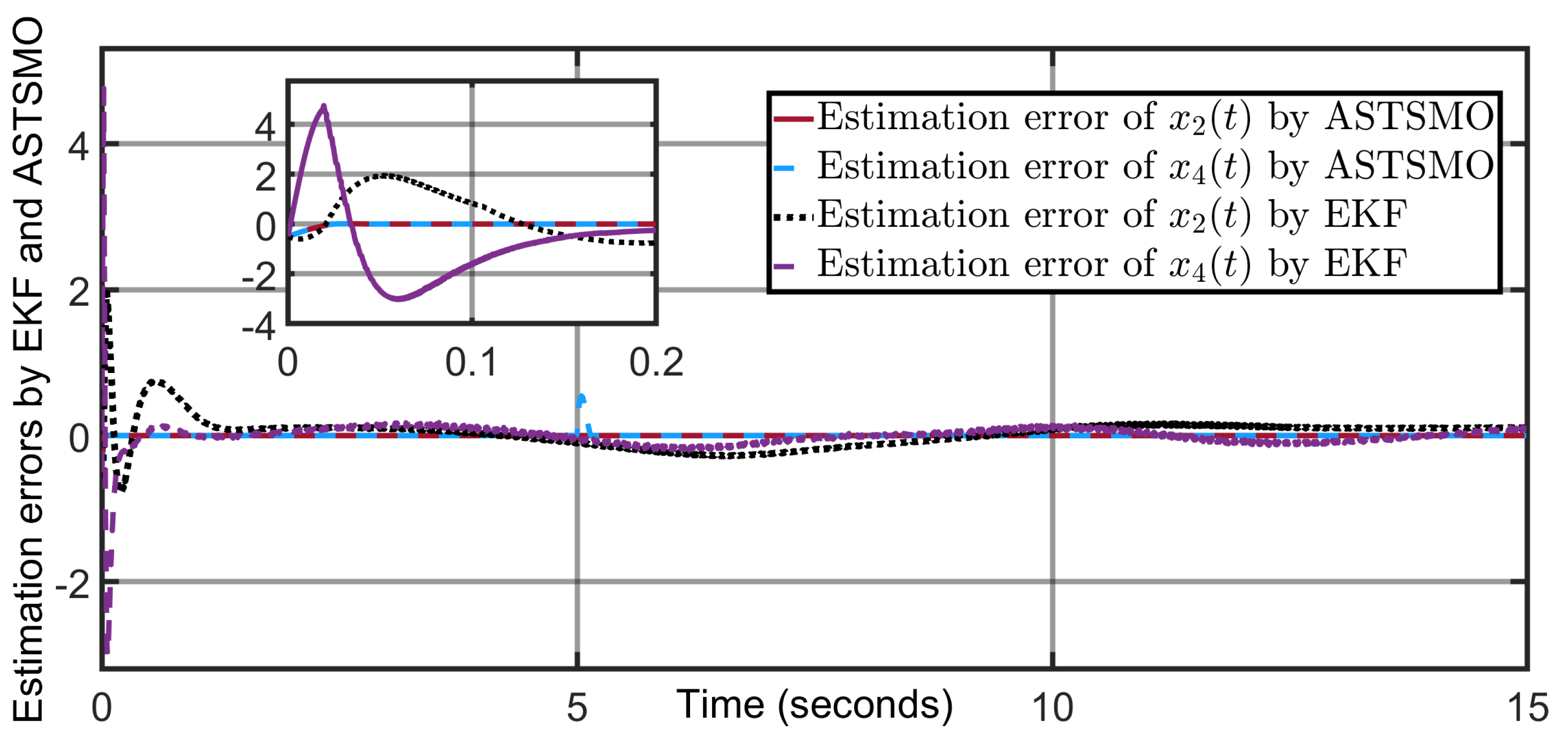
In order to compare the performance of our proposed cascade-adaptive super-twisting sliding-mode observer (STD+ASTSMO) to the standard Extended Kalman Filter (EKF), we have carried out new numerical simulation by implementing and simultaneously simulating our proposed cascade observer (STD+ASTSMO) and the standard EKF for state/disturbance estimation in the exoskeleton system under identical disturbance and noise conditions.

In fact, we implemented an Extended Kalman Filter (EKF) with augmented state ${[x_1,x_2,x_3,x_4,d_1,d_2]}^T$ and augmented dynamics using the Control System Toolbox (Bloc Simulink “Extended Kalman Filter”) with a discrete sampling time of $T_s=1$ ms ($F_s=1$ KHz) on the nonlinear two-DOF model. The measurements $[x_1={\theta }_1,x_3={\theta }_2]$ were sampled through a Zero-Order Hold and corrupted with Gaussian noise. Three scenarios were tested in the same disturbance and noise conditions (step and varying torque disturbances) and Gaussian measurement noise. The covariance matrices were conservatively tuned ($Q=diag[{10}^{-6},5.{10}^{-4},{10}^{-6},5.{10}^{-4}]$, $R={10}^{-2}{I}_2$).

The simulation results show a comparison in terms of state estimation performance (Figure 30 and Figure 31) and disturbance estimation (Figure 32) between our proposed cascade-adaptive super-twisting sliding-mode observer (STD+ASTSMO) and the standard Extended Kalman Filter (EKF).

The results show that, while the EKF is able to track the measured states, it struggles to reconstruct unknown disturbances. In contrast, the proposed cascade observer provides a robust finite-time estimation of disturbances with faster transient response. However, Kalman filters are efficient in appropriate applications such as linear or linearized systems.

6.6. Discussion and Perspectives on Real-Time Hardware Implementation

The present work focuses on the theoretical development and simulation validation of the proposed cascade-observer-based control algorithm. The experimental validation will be considered in our future works, where we will investigate the real-time implementation on embedded hardware such as field programmable gate array (FPGA) or microprocessor-based systems (such as microcontrollers).

Indeed, FPGA implementation of sliding-mode controllers and sliding-mode observers was successfully realized in several existing works in different applications, such as robotic systems [24], electrical systems [25,26], etc. FPGA choice is relevant for Parallel Processing (the main characteristic in FPGAs): the cascade observer structure-based controller benefits from parallel computation of the STD, ASTSMO, and SMC controller. Moreover, FPGAs provide deterministic execution times that are crucial for real-time control and are able to handle high sampling rates (>1 kHz) required for smooth control [24,26].

Microprocessor-based systems such as microcontrollers are generally used for less demanding applications and may suffice for moderate control bandwidths; however, modern high-performance microprocessors could also implement this algorithm.

Experimental strategies and plans of validation will be addressed in our future works using a detailed analysis of the algorithm’s computational steps, execution time estimation, and suitability for real-time embedded platforms.

7. Conclusions

In this paper, we have developed a new output-feedback tracking control scheme for a two-DOF lower-limb exoskeleton system. First, based on the joint angle measurements, a super-twisting differentiator (STD) was designed to estimate the angular velocity states. Second, the estimates of the latter observer were used by an adaptive super-twisting sliding-mode observer (ASTSMO), whose objective is to reconstruct the external load torque disturbance. Third, the estimated states and disturbances were integrated into a sliding-mode controller that was designed to ensure tracking control objectives despite the presence of unknown inputs. Numerical simulations realized with Matlab/Simulink software demonstrated the excellent estimation performance of the designed observers and that robust tracking control objectives are achieved with very good accuracy and fast convergence.

References

1. Abdallah, C.; Dawson, D.; Dorato, P.; Jamshidi, M. Survey of robust control for rigid robots. IEEE Control Syst. Mag. 1991, 11, 24–30. [Google Scholar]
2. Guo, Z.; Yu, H.; Yin, Y. Developing a mobile lower limb robotic exoskeleton for gait rehabilitation. J. Med. Devices 2014, 8, 044503. [Google Scholar] [CrossRef]
3. Chen, Z.; Li, Z.; Chen, C. Disturbance observer-based fuzzy control of uncertain MIMO mechanical systems with input nonlinearities and its application to robotic exoskeleton. IEEE Trans. Cybern. 2017, 47, 984–994. [Google Scholar] [CrossRef]
4. Chen, C.; Du, Z.; He, L.; Wang, J.; Wu, D.; Dong, W. Active disturbance rejection with fast terminal sliding mode control for a lower limb exoskeleton in swing phase. IEEE Access 2019, 7, 72343–72357. [Google Scholar] [CrossRef]
5. Estrada, A.; Plestan, F. Second order sliding mode output feedback control with switching gains—Application to the control of a pneumatic actuator. J. Frankl. Inst. 2014, 351, 2335–2355. [Google Scholar] [CrossRef]
6. Liu, Z.; Liu, J.; Zhang, O.; Zhao, Y.; Chen, W. Adaptive Disturbance Observer-Based Fixed-Time Tracking Control for Uncertain Robotic Systems. IEEE Trans. Ind. Electron. 2024, 71, 14823–14831. [Google Scholar] [CrossRef]
7. Tran, T.; Duong, V.; Nguyen, H.; Nguyen, T. Terminal super-twisting sliding mode based on high order sliding mode observer for two DOFs lower limb system. Meas. Control 2023, 56, 1455–1470. [Google Scholar] [CrossRef]
8. Zhang, J.; Gao, W.; Guo, Q. Extended State Observer-Based Sliding Mode Control Design of Two-DOF Lower Limb Exoskeleton. Actuators 2023, 12, 402. [Google Scholar] [CrossRef]
9. Long, Y.; Peng, Y. Extended State Observer-Based Nonlinear Terminal Sliding Mode Control with Feedforward Compensation for Lower Extremity Exoskeleton. IEEE Access 2022, 22, 8643–8652. [Google Scholar] [CrossRef]
10. Bembli, S.; Khraief Haddad, N.; Belghith, S. A Robust Model Free Terminal Sliding Mode with Gravity Compensation Control of a 2 DoF Exoskeleton-Upper Limb System. J. Control. Autom. Electr. Syst. 2021, 8, 632–641. [Google Scholar] [CrossRef]
11. Sun, Z.; Qiu, J.; Zhu, J.; Li, S. A composite position control of flexible lower limb exoskeleton based on second-order sliding mode. Nonlinear Dyn. 2022, 111, 1657–1666. [Google Scholar] [CrossRef]
12. Aole, S.; Elamvazuthi, I.; Waghmare, L.; Patre, B.; Meriaudeau, F. Improved active disturbance rejection control for trajectory tracking control of lower limb robotic rehabilitation exoskeleton. Sensors 2020, 20, 3681. [Google Scholar] [CrossRef]
13. Aole, S.; Elamvazuthi, I.; Waghmare, L.; Patre, B.; Meriaudeau, F. Non-linear active disturbance rejection control for upper limb rehabilitation exoskeleton. Proc. Inst. Mech. Eng. Part I J. Syst. Control Eng. 2021, 235, 606–632. [Google Scholar] [CrossRef]
14. Aole, S.; Elamvazuthi, I.; Waghmare, L.; Patre, B.; Bhaskarwar, T.; Meriaudeau, F.; Su, S. Active disturbance rejection control based sinusoidal trajectory tracking for an upper limb robotic rehabilitation exoskeleton. Appl. Sci. 2022, 12, 1287. [Google Scholar] [CrossRef]
15. Ahmed, S.; Wang, H.; Tian, Y. Robust Adaptive Fractional-Order Terminal Sliding Mode Control for Lower-Limb Exoskeleton. Asian J. Control 2019, 22, 473–482. [Google Scholar] [CrossRef]
16. Pérez-San Lázaro, R.; Salgado, I.; Chairez, I. Adaptive sliding-mode controller of a lower limb mobile exoskeleton for active rehabilitation. ISA Trans. 2021, 109, 218–228. [Google Scholar] [CrossRef]
17. Aly, A.; Vu, M.; El-Sousy, F.; Hsia, K.H.; Alotaibi, A.; Mousa, G.; Le, D.N.; Mobayen, S. Adaptive Neural Network-Based Fixed-Time Tracking Controller for Disabilities Exoskeleton Wheelchair Robotic System. Mathematics 2022, 10, 3853. [Google Scholar] [CrossRef]
18. Bowen, Z.; Tong, W.; Tianqi, W. Adaptive Neural Network Control for Exoskeleton Motion Rehabilitation Robot with Disturbances and Uncertain Parameters. IEEE Access 2023, 91, 75497. [Google Scholar] [CrossRef]
19. Moreno, J.; Osorio, M. Strict Lyapunov functions for the super-twisting algorithm. IEEE Trans. Autom. Control 2012, 57, 1035–1040. [Google Scholar] [CrossRef]
20. Wang, L.; Du, Z.; Dong, W.; Shen, Y.; Zhao, G. Full-state feedback control of flexible-joint robots with singular perturbation technique. IEEE Trans. Control Syst. Technol. 2020, 28, 2415–2422. [Google Scholar]
21. Yan, T.; Cempini, M.; Oddo, C.; Vitiello, N. Review of assistive strategies in powered lower-limb orthoses and exoskeletons. Robot. Auton. Syst. 2015, 64, 120–136. [Google Scholar] [CrossRef]
22. Rigatos, G.; Abbaszadeh, M.; Pomares, J. Flatness-based control and Kalman Filter-based disturbance observer for robotic exoskeletons under time-delayed contact forces. Adv. Control Appl. Eng. Ind. Syst. 2022, 4, e100. [Google Scholar] [CrossRef]
23. Wang, Y.; Wang, H.; Tian, Y. Nonlinear disturbance observer based flexible-boundary prescribed performance control for a lower limb exoskeleton. Int. J. Syst. Sci. 2021, 52, 1001–1017. [Google Scholar] [CrossRef]
24. Hsu, C.; Lee, B. FPGA-based adaptive PID control of a DC motor driver via sliding-mode approach. Expert Syst. Appl. 2011, 38, 11866–11872. [Google Scholar] [CrossRef]
25. Gürsoy, H.; Efe, M. Control System Implementation on an FPGA Platform. IFAC-PapersOnLine 2016, 29, 425–430. [Google Scholar] [CrossRef]
26. Naouar, M.; Ben Hania, B.; Slama-Belkhodja, I.; Monmasson, E.; Naassani, A. FPGA-based sliding mode direct control of single phase PWM boost rectifier. Math. Comput. Simul. 2013, 91, 249–261. [Google Scholar] [CrossRef]
Figure 1. The two-DOF lower-limb exoskeleton scheme.
Actuators 14 00503 g001
Figure 2. Cascade super-twisting observer-based output-feedback sliding-mode controller applied to the exoskeleton system, including external load torque perturbations.
Actuators 14 00503 g002
Figure 3. Estimation errors of the angular velocity states x 2 = θ ˙ 1 and x 4 = θ ˙ 2 using the proposed super-twisting differentiator.
Actuators 14 00503 g003
Figure 4. Estimation of the angular velocity state x 2 = θ ˙ 1 using the proposed super-twisting differentiator (STD).
Actuators 14 00503 g004
Figure 5. Estimation of the angular velocity state x 4 = θ ˙ 2 using the proposed super-twisting differentiator (STD).
Actuators 14 00503 g005
Figure 6. Estimation of the disturbance d 1 ( t ) by the proposed adaptive super-twisting sliding-mode observer (ASTSMO).
Actuators 14 00503 g006
Figure 7. Estimation of the disturbance d 2 ( t ) by the proposed adaptive super-twisting sliding-mode observer (ASTSMO).
Actuators 14 00503 g007
Figure 8. Tracking control errors x 1 x 1 r e f and x 3 x 3 r e f using the proposed super-twisting observer-based sliding-mode controller.
Actuators 14 00503 g008
Figure 9. Tracking control for joint angle x 1 = θ 1 using the proposed super-twisting observer-based sliding-mode controller.
Actuators 14 00503 g009
Figure 10. Tracking control for joint angle x 3 = θ 2 using the proposed super-twisting observer-based sliding-mode controller.
Actuators 14 00503 g010
Figure 11. Torque control signal u 1 .
Actuators 14 00503 g011
Figure 12. Torque control signal u 2 .
Actuators 14 00503 g012
Figure 13. Estimation of the sinusoidal disturbance d 1 ( t ) = 2 sin ( 2 π t ) + 1 by the proposed adaptive super-twisting sliding-mode observer (ASTSMO).
Actuators 14 00503 g013
Figure 14. Estimation of the sinusoidal disturbance d 2 ( t ) = 4 sin ( 2 π 10 t ) + 2 by the proposed adaptive super-twisting sliding-mode observer (ASTSMO).
Actuators 14 00503 g014
Figure 15. Estimation of the sinusoidal disturbance d 1 ( t ) by the proposed adaptive super-twisting sliding-mode observer (ASTSMO) in presence of Gaussian noise.
Actuators 14 00503 g015
Figure 16. Estimation of the step disturbance d 2 ( t ) by the proposed adaptive super-twisting sliding-mode observer (ASTSMO) in presence of Gaussian noise.
Actuators 14 00503 g016
Figure 17. Tracking control errors x 1 x 1 r e f and x 3 x 3 r e f using the proposed super-twisting observer-based sliding-mode controller in presence of Gaussian noise.
Actuators 14 00503 g017
Figure 18. Tracking control for joint angle x 1 = θ 1 using the proposed super-twisting observer-based sliding-mode controller in presence of Gaussian noise.
Actuators 14 00503 g018
Figure 19. Tracking control for joint angle x 3 = θ 2 using the proposed super-twisting observer-based sliding-mode controller in presence of Gaussian noise.
Actuators 14 00503 g019
Figure 20. Torque control signal u 1 in presence of Gaussian noise.
Actuators 14 00503 g020
Figure 21. Torque control signal u 2 in presence of Gaussian noise.
Actuators 14 00503 g021
Figure 22. Progressive and sudden changes in shank segment mass m 2 ( t ) .
Actuators 14 00503 g022
Figure 23. Control input signals under mass variation in shank segment.
Actuators 14 00503 g023
Figure 24. Tracking errors and estimation errors under mass variation in shank segment.
Actuators 14 00503 g024
Figure 25. Torque control signals u 1 ( t ) and u 2 ( t ) with sampling rate F s = 100 Hz (sampling time T s = 10 ms).
Actuators 14 00503 g025
Figure 26. Torque control signals u 1 ( t ) and u 2 ( t ) with sampling rate F s = 10 KHz (sampling time T s = 0.1 ms).
Actuators 14 00503 g026
Figure 27. Control input signal u 2 ( t ) ) and its high-frequency content under control parameters k 1 = k 2 = 10 , μ = 0.01 in the presence of measurement Gaussian noise.
Actuators 14 00503 g027
Figure 28. Control input signal u 2 ( t ) ) and its high-frequency content under control parameters k 1 = k 2 = 10 , μ = 0.001 in the presence of measurement Gaussian noise.
Actuators 14 00503 g028
Figure 29. Control input signal u 2 ( t ) ) and its high-frequency content under control parameters k 1 = 4 , k 2 = 7 , μ = 0.05 in the presence of measurement Gaussian noise.
Actuators 14 00503 g029
Figure 30. State estimation comparison between the proposed cascade-adaptive super-twisting sliding-mode observer (STD+ASTSMO) and the standard Extended Kalman Filter (EKF).
Actuators 14 00503 g030
Figure 31. State estimation errors using the proposed cascade-adaptive super-twisting sliding-mode observer (STD+ASTSMO) and the standard Extended Kalman Filter (EKF).
Actuators 14 00503 g031
Figure 32. Disturbance estimation comparison between the proposed cascade-adaptive super-twisting sliding-mode observer (STD+ASTSMO) and the standard Extended Kalman Filter (EKF).
Actuators 14 00503 g032