Fault Diagnosis Method of Permanent Magnet Synchronous Motor Based on WCNN and Few-Shot Learning

Abstract

With the continuous development of actuator technology, the Electro-Mechanical Actuator (EMA) is gradually becoming the first choice in the aviation field. Permanent Magnet Synchronous Motor (PMSM) is one of the core components of EMA, and its healthy state determines the working performance of EMA. In this paper, the interturn short-circuit fault of PMSM is taken as the typical fault, and a new fault diagnosis framework is proposed based on a wide-kernel convolutional neural network (WCNN) and few-shot learning. Firstly, the wide convolution kernel is added as the first layer to extract short-time features while automatically learning deeply oriented features oriented to diagnosis and removing useless features. Then, the twin neural network is introduced to establish a wide kernel convolutional neural network, which can also achieve good diagnostic results under a few-shot learning framework. The effectiveness of the proposed method is verified by the general data set. The results show that the accuracy of few-shot learning is 9% higher than that of WCNN when the fault data are small. Finally, a fault test platform was built for EMA to collect three-phase current data under different fault states, and the collected data were used to complete the fault diagnosis of PMSM. With limited data, the accuracy of few-shot learning increased by 8% on average compared with WCNN, which has good engineering value.

1. Introduction

The servo actuating system is the actuator of the automatic flight control system. When the aircraft needs to change its attitude and trajectory, it is the Servo actuating system that drives the steering plane to deflect, thus completing the control of the aircraft [1,2,3]. With the rapid development of aircraft technology to MEA (More Electrical Aircraft) and AEA (All Electric Aircraft), electrification technology is applied more and more widely in aircraft, and the key components of aircraft are developing towards multi-electric. As with the engine, braking system, and other important systems, the servo actuating system also needs to develop towards high output, high power, high reliability, short response time, and so on, and constantly break through the bottleneck of key technologies. Therefore, the new EPA (Electric Powered Actuator) is designed to replace the traditional hydraulic actuator system as the actuator of the rudder of new aircraft [4,5,6,7]. There are two types of EPA: EMA (Electro-Mechanical Actuator) and EHA (Electro-Hydraulic Actuator). Compared with EHA, EMA has no hydraulic mechanism and is characterized by simple structure, high power density, and easy maintenance. Therefore, it will be widely used in various driving devices of AEA and MEA, such as electric brakes, landing gear retraction, steering gear steering, and blade expansion, and become the main aviation servo actuation system [8,9,10].

Due to the complex system of EMA and diverse operating conditions, it often works in harsh environments, so it is inevitable that faults will occur [11], especially PMSM (Permanent Magnet Synchronous Motor) in EMA. PMSM is the core component of EMA, and the control of EMA is essentially the control of PMSM. Therefore, the performance of PMSM directly determines the performance of EMA. Once the PMSM fails, EMA often fails to work, so it is urgent to study the fault diagnosis methods of PMSM [12,13,14].

Common failures of PMSM include electrical failures, magnetic failures, and mechanical failures. The main fault is an electrical fault, especially the stator winding turns short circuit fault. When the turn-to-turn short circuit occurs, the current of the short circuit phase increases, so that the coil is heating, serious burn motor. At the same time, the three-phase current of the motor is no longer balanced, which makes the output torque of the motor fluctuate and cannot be started with load when it is serious. Therefore, this paper studies the interturn short-circuit fault as a typical fault of PMSM [15,16].

With the advent of the era of big data, deep learning has been widely used in the field of fault diagnosis [17,18,19]. Deep learning can process massive data, which is the biggest advantage of deep learning but also its weakness. Because in the development and testing phase of the device, it is difficult to find a lot of data to train the deep learning model. Therefore, a deep learning method that can effectively complete fault diagnosis even when the fault data sample is small is needed.

The main contributions of this paper are as follows:

• Modeling of PMSM interturn short circuit fault was completed. The inter-turn short circuit fault simulation of a permanent magnet synchronous motor is carried out. The inter-turn short circuit fault of the motor is simulated, and the control system model of EMA is studied. Finally, it is determined that the three-phase current signal of the permanent magnet synchronous motor in EMA is the most suitable fault parameter.
• A deep learning fault diagnosis model suitable for small fault samples is designed, which can effectively complete fault diagnosis even when the training sample is small.
• A test platform is designed for fault data collection. On this basis, current data of EMA under different degrees of interturn short circuit were collected, and the deep learning framework designed above was used for fault diagnosis.

The content of this paper is organized as follows: In Section 2, the fault diagnosis method that can meet the needs of this paper is studied, and a wide-core convolutional neural network is designed. The twin neural network is introduced, and the two are combined to form a small sample learning framework for fault diagnosis. In Section 3, the general fault data set is used to verify the algorithm of the learning framework obtained in the bottom section. The results show that the small sample learning framework has a significant improvement effect compared with the wide kernel convolutional neural network when the training samples are small. At the same time, it has certain anti-noise performance. In Section 4, the inter-turn short circuit fault modeling of a permanent magnet synchronous motor is carried out. Then, the test platform is built and the fault diagnosis method is verified. The small sample learning framework designed in Section 2 is used to complete the fault diagnosis of EMA. By comparing with the diagnostic accuracy of 1DCNN and WCNN, it is proved that the fault diagnosis method proposed in this paper has great advantages under small sample conditions.

2. The Proposed Fault Diagnosis Framework

Convolutional neural networks are widely used in image processing, speech recognition, and fault diagnosis due to their powerful data processing capability [20,21,22]. Here, we also choose CNN as the basis of the fault diagnosis method.

2.1. CNN

A convolutional neural network is a deep learning model that is especially suitable for processing data with grid structure, such as images. It imitates some characteristics of the biological vision system and has achieved great success in the field of computer vision. The main components of CNN include the following:

• Convolution layer: used to detect the spatial hierarchical pattern in the input.
• Pooling layer: It is usually used to reduce the spatial dimension of data representation, thereby reducing the number of parameters and the amount of calculation.
• Fully connected layer: It is used to map the features extracted by the convolutional layer and the pooling layer to the high-dimensional feature space and finally make a classification decision.

2.1.1. 1DCNN

1DCNN (1-Dimensional Convolutional Neural Networks) is a variant of convolutional neural networks, which is specially used to process one-dimensional sequence data. Unlike traditional 2D CNN, which is used to process two-dimensional image data, 1D CNN can process time series data, one-dimensional signals (such as audio signals or electrocardiogram ECG), etc.

The main feature of 1DCNN is that they use one-dimensional convolution kernels to slide and process data rather than using two-dimensional convolution kernels like 2D CNN. Such one-dimensional convolution kernels can capture local correlations in time or space dimensions, which is very useful for many tasks.

The basic architecture of 1DCNN is similar to 2DCNN, including the following parts:

• Convolution layer: A one-dimensional filter (convolution kernel) slides over the input data to detect patterns at specific locations. Each convolution kernel corresponds to a specific pattern. After multiple sets of convolution kernels, a variety of different local features can be captured.
• Activation function: ReLU (Rectified Linear Unit) is usually used as the activation function to introduce nonlinear characteristics.
• The pooling layer: used to reduce the spatial dimension of the output; the common ones are max pooling and average pooling.
• Fully connected layer: at the end of the network, it is used to map the features extracted by the convolutional layer to specific tasks, such as classification or regression.

2.1.2. WCNN

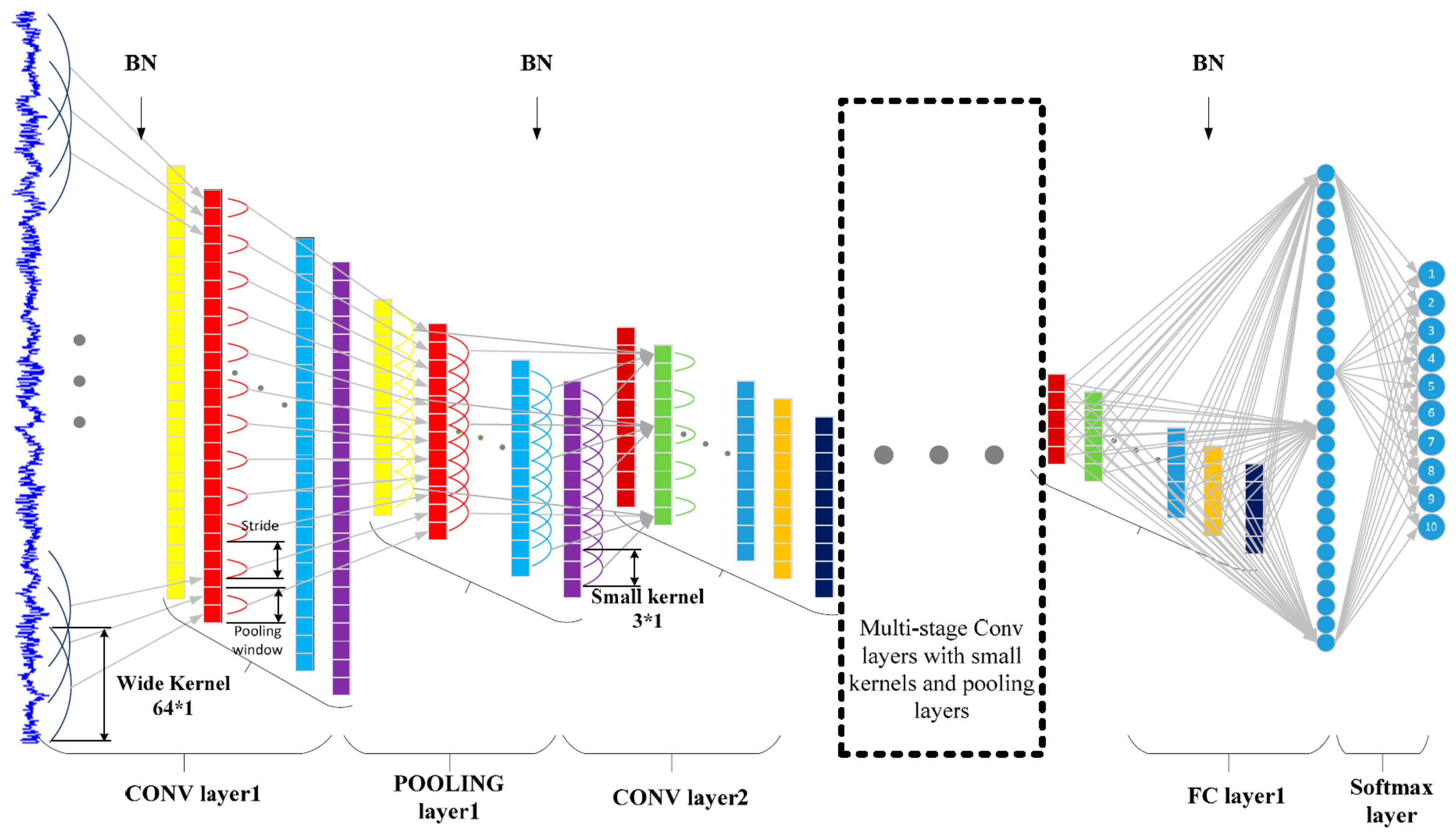
Since the signals processed by the fault diagnosis are one-dimensional signals, this paper designs the WCNN, as shown in Figure 1, whose structure is characterized by a 64 × 1 wide convolutional kernel as the first layer and 3 × 1 kernels as the subsequent layers. The function of the first wide convolution kernel is to extract short-time features, which is similar to the short-time Fourier transform. At the same time, it can automatically learn features oriented to diagnosis and automatically remove features that are not helpful to diagnosis. However, the convolution kernel size of other convolutional layers except the first layer is set to 3 × 1, which not only deepens the number of network layers and enhances the expression ability of the network but also reduces network parameters and avoids overfitting.

In addition, a BN (Batch Normalization) layer is added between the convolution layer and the activation layer and between the full connection layer and the activation layer, which can reduce the internal covariate transfer, improve the training efficiency of the network, and enhance the generalization ability of the network. The main operation step is to subtract the mean value of mini-batch from the input of the convolutional layer or full connection layer and then divide the standard deviation. This is similar to a standardized operation, so it can accelerate the training. However, this will limit the input value to a narrow range and reduce the expressiveness of the network. Therefore, the normalized values are re-multiplied by a scaling quantity $\mathsf{\gamma }$ and added with a bias quantity $\mathsf{\beta }$ to enhance the expression.

2.2. Few-Shot Learning Framework

When the data set is limited, using a small sample learning algorithm can effectively avoid the risk of model overfitting. Traditional deep learning models require a large amount of data for training in order to learn enough features and improve generalization ability. However, when the data are small, these models are easy to over-fit the noise or specific patterns in the training data. Small sample learning reduces the dependence on specific samples through a more concise model architecture or through specific regularization methods, so it can better capture the common patterns in the data and improve the accuracy of the model. Small sample learning algorithms usually rely on transfer learning, meta-learning, and other technologies to compensate for the lack of data by using prior knowledge (such as existing models, pre-trained feature representations, etc.). This prior knowledge may come from the pre-training model of large-scale data sets or the feature representation obtained from similar tasks. By migrating this existing knowledge to new small data sets, the model can learn quickly and accurately classify or predict, even if there is only a small amount of new data. In small sample learning, model design usually focuses on improving data utilization efficiency.

Compared with traditional deep learning models, small sample learning models are usually smaller and simpler, so they have better robustness and generalization. Due to the low complexity of the model, it is not easily disturbed by noise or unimportant features in the training data. Small sample learning algorithms usually pay more attention to features with higher information content without wasting resources on irrelevant or redundant features. By focusing on the most important features, the model can learn more effectively, thereby improving accuracy. Because the model can effectively self-adjust in the case of small samples, it can quickly fine-tune in the face of new data distributions or tasks without retraining a large amount of data. This fast adaptability further improves the accuracy of the model under small sample conditions.

Few-shot learning refers to the ability of machine learning models to learn and generalize to new samples with only a small number of labeled samples. This learning method is particularly important in reality, because it is difficult to obtain a large amount of annotated data in many practical application scenarios. The general strategy of small sample learning can be summarized as the following aspects. Data augmentation: By transforming and expanding the original data, more training samples are generated. Improve the generalization ability of the model and reduce the risk of overfitting. Transfer learning: Based on the model pre-trained on large-scale data sets, it is transferred to a small sample learning task and fine-tuned. Using the feature representation ability that the pre-trained model has learned, the sample size required for training in small sample tasks is reduced. Meta-learning: Meta-learning attempts to train a model that can learn and adapt quickly when given small sample data for new tasks. By performing gradient updates on multiple tasks, the model can achieve better performance with fewer gradient update steps when a new task is given. It provides a new way of learning. Few-shot/Zero-shot learning: Few-shot learning attempts to learn from a small number of samples and generalize to new samples; zero-shot learning goes further and does not rely on samples of any target category. Regularization: Reduce the risk of overfitting by limiting the complexity of the model. The generalization ability of the model in the case of small samples is improved by methods such as Weight Decay, Dropout, and Early Stopping. Model structure design: Reduce the number of layers and neurons to reduce the complexity of the model. Structures with intrinsic regularization effects are used, such as the convolutional neural network (CNN) and recurrent neural network (RNN). Ensemble Learning: train multiple neural network models and fuse their prediction results. Improve the generalization ability and stability of the model and reduce the risk of overfitting. Feature transfer and multi-task learning: Feature transfer refers to the use of pre-training models in related fields to extract features and then fine-tune them on small sample data sets. Multi-task learning refers to sharing the underlying feature representation by learning multiple related tasks at the same time to improve the generalization ability of the model.

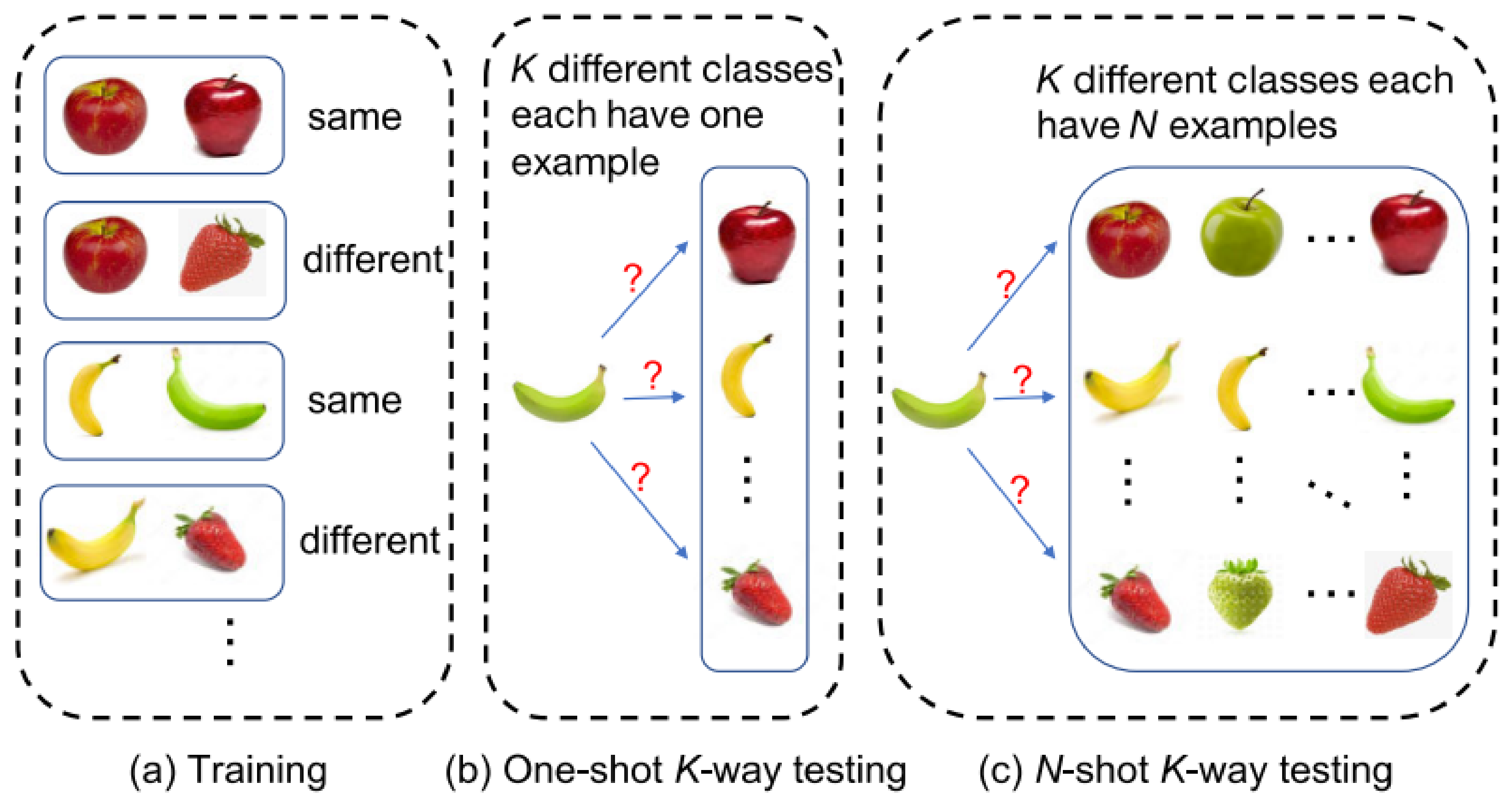
The general strategy of few-shot learning is shown in Figure 2, which is based on multiple applications of one-shot learning [23]. First, it trains the model using a collection of sample pairs of the same or different categories. The input is a pair of samples of the same or different class $({\mathrm{x}}_1^{\mathrm{i}},{\mathrm{x}}_2^{\mathrm{i}})$, and the output is the probability $\mathrm{p}({\mathrm{x}}_1^{\mathrm{i}},{\mathrm{x}}_2^{\mathrm{i}})$ that the two input samples are the same. Unlike traditional classification, the performance of few-shot learning is usually measured by the N-shot K-way test.

A one-shot K-way test gives a classification of test sample $\widehat{\mathrm{x}}$ and a set of supporting $\mathrm{S}$, which contains $\mathrm{K}$ samples. Each sample has a different label $\mathrm{y}$, as shown in Formula (1). It then classifies the test samples according to the most similar samples in the support set, as shown in Formula (2). In the N-shot K-way test, a support set is given, which consists of $\mathrm{K}$ distinct classes, each with $\mathrm{N}$ samples $({\mathrm{S}}_1,\dots ,{\mathrm{S}}_{\mathrm{N}})$. Then, the model needs to determine which support set class the test sample belongs to, as shown in Formula (3).

$$\mathrm{S}=\left\{\left({\mathrm{x}}_1,{\mathrm{y}}_1\right),\dots ,({\mathrm{x}}_{\mathrm{K}},{\mathrm{y}}_{\mathrm{K}})\right\}$$

(1)

$$\mathrm{C}\left(\widehat{\mathrm{x}},\mathrm{S}\right)=\mathrm{a}\mathrm{r}\mathrm{g}\underset{\mathrm{C}}{\max }\left(\mathrm{P}\left(\widehat{\mathrm{x}},{\mathrm{x}}_{\mathrm{c}}\right)\right),{\mathrm{x}}_{\mathrm{c}}\in \mathrm{S}$$

(2)

$$\mathrm{C}\left(\widehat{\mathrm{x}},\left({\mathrm{S}}_1,\dots ,{\mathrm{S}}_{\mathrm{N}}\right)\right)=\mathrm{a}\mathrm{r}\mathrm{g}\underset{\mathrm{C}}{\max }\left(\sum _{\mathrm{n}=1}^{\mathrm{N}}\mathrm{P}\left(\widehat{\mathrm{x}},{\mathrm{x}}_{\mathrm{c}\mathrm{n}}\right)\right),{\mathrm{x}}_{\mathrm{c}\mathrm{n}}\in {\mathrm{S}}_{\mathrm{n}}$$

(3)

2.3. Few-Shot Learning Framework Based on WCNN

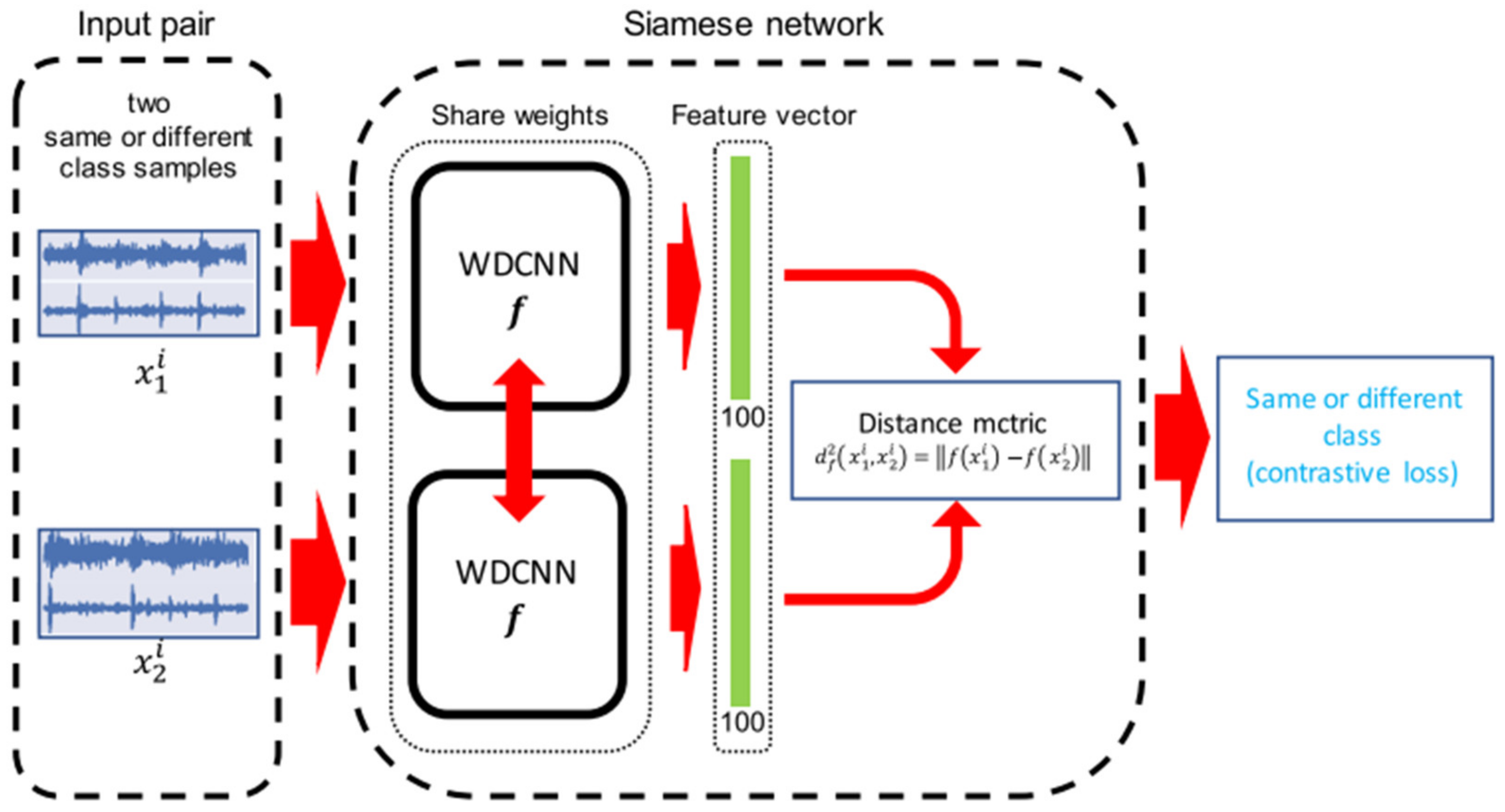
Based on the WCNN and the few-shot learning framework mentioned above, the Siamese Neural Network (SNN) is introduced in this section to build a few-shot learning model for fault diagnosis [24]. In this network model, two identical WCNN networks are established using the same network architecture and shared weights, as shown in Figure 3.

The input of the framework is a pair of samples of the same or different class, and features can be extracted from the original fault signals directly using WCNN, which is the so-called end-to-end deep learning method [25]. The output is the “distance” between the feature vector output and the twin WCNN, according to which the input sample pair can be judged to be similar or not similar.

Let M denote the size of a small batch and i denote the i-th small batch. The twin sub-network is optimized based on the distance measure between its outputs. Let $t_j=y(x_{1j}^i,x_{2j}^i)$ be a vector of length M containing a small batch of labels. When $x_{1j}^i$ and $x_{2j}^i$ are from the same fault category, we set $t_j=1$; otherwise, let $t_j=0$. Where j is the j-th sample pair from the i-th small batch. The loss function is a regularized cross entropy. In addition, the network is optimized by the Adam optimizer, which calculates the individual adaptive learning rate for each parameter.

We use multiple one-shot K-way tests to simulate the N-shot K-way test. For the five-shot N-way test task, it is the same as the one-shot K-way test task. We repeat five one-shot K-way tests as five data support sets, and each data support set S is randomly selected from the training data. After five times of the one-shot K-way test, five probability vectors are obtained, and then the maximum probability sum of the same label is calculated.

3. Experimental Verification Based on Conventional Data Sets

In electric motors, various types of faults can impact their performance and lifespan. Among them, bearing faults are one of the most common types, accounting for approximately 40% to 50% of all motor faults. This high occurrence rate makes bearing faults an important focus for studying motor reliability and maintenance. Bearing faults can manifest in various modes, such as pitting, wear, fatigue damage, and poor lubrication. These different types of faults cause distinct vibration and noise characteristics, providing a rich data set and test cases for developing and validating fault detection and diagnostic algorithms. Bearing faults typically have a significant impact on the overall performance of the motor, such as increasing vibration levels, overheating, reducing energy efficiency, and even causing total motor failure. Thus, timely identification and diagnosis of bearing faults are crucial to ensuring the reliable operation of electric motors. Since the signal characteristics of bearing faults are relatively distinct and easy to capture, using such data can effectively validate the performance and robustness of fault detection and diagnostic algorithms. Through machine learning and signal processing techniques, early detection of bearing faults can be achieved, thereby reducing maintenance costs and extending the equipment’s service life. The bearing data set is used to train the small sample learning framework, and finally the interturn short circuit fault diagnosis is solved by the framework when the number of samples is small. The selection of bearing data sets is mainly due to its advantages in the following aspects, performance evaluation: By using data sets with known faults, the effectiveness and accuracy of different prediction algorithms can be tested and verified. Model training and optimization: Data sets can be used to train machine learning models to help optimize model parameters and improve the accuracy of fault prediction.

In order to verify whether the few-shot diagnosis framework designed in this paper can achieve good results, the bearing fault data set of Case Western Reserve University (CWRU), the authoritative data set in the field of fault diagnosis, is used for algorithm verification in this excerpt. Here, bearing fault data at the 12 k driving end (sampling frequency of sensor is 12 KHz) are selected as the original experimental data. As shown in

Table 1. Description of rolling bearing data sets.

Fault Location		NRM	Ball			Inner Race			Outer Race			Load
Fault size (mil)		0	7	14	21	7	14	21	7	14	21
labels		1	2	3	4	5	6	7	8	9	10
Data set A	Train	600	600	600	600	600	600	600	600	600	600	1
	Test	25	25	25	25	25	25	25	25	25	25
Data set B	Train	600	600	600	600	600	600	600	600	600	600	2
	Test	25	25	25	25	25	25	25	25	25	25
Data set C	Train	600	600	600	600	600	600	600	600	600	600	3
	Test	25	25	25	25	25	25	25	25	25	25
Data set D	Train	1800	1800	1800	1800	1800	1800	1800	1800	1800	1800	1, 2, 3
	Test	75	75	75	75	75	75	75	75	75	75

, there are four types of bearing fault locations: normal, ball fault, inner race fault, and outer race fault. Each fault type contains three types: seven mils, fourteen mils, and twenty-one mils, so we have a total of ten types of fault labels. Each fault label contains three types of loads of 1, 2, and 3 hp (motor speeds of 1772, 1750, and 1730 RPM, respectively).

Each sample is extracted from two vibration signals, respectively. We use half of the vibration signals to generate training samples and the other half to generate test samples. Training samples are generated by sliding Windows with a size of 2048 points and a sliding step size of 80 points, and test samples are generated by sliding Windows of the same size without overlapping sliding. Data sets A, B, and C contain 600 training samples and 25 test samples, respectively, under different working conditions of 1, 2, and 3 HP. Data set D contains a total of 1800 training samples and 75 test samples under three load conditions.

3.1. WCNN Model Parameter Design Criteria

Table 2. Structural parameters of WCNN model.

Number	Layer Type	Kernel Size/Stride	Kernel Number	Output Size (Width × Depth)	Padding
1	Convolution 1	64 × 1/16 × 1	16	128 × 16	Yes
2	Pooling 1	2 × 1/2 × 1	16	64 × 16	No
3	Convolution 2	3 × 1/1 × 1	32	64 × 32	Yes
4	Pooling 2	2 × 1/2 × 1	32	32 × 32	No
5	Convolution 3	3 × 1/1 × 1	64	32 × 64	Yes
6	Pooling 3	2 × 1/2 × 1	64	16 × 64	No
7	Convolution 4	3 × 1/1 × 1	64	16 × 64	Yes
8	Pooling 4	2 × 1/2 × 1	64	8 × 64	No
9	Convolution 5	3 × 1/1 × 1	64	6 × 64	No
10	Pooling 5	2 × 1/2 × 1	64	3 × 64	No
11	Fully-connected	100	1	100 × 1
12	Softmax	10	1	10

details the setup of WCNN network architecture, which first uses wide cores to extract features and then small cores to obtain better feature representation. This design strategy is due to the fact that it is not practical to design a model with all the small cores and that the layer 1 small cores are easily disturbed by the high frequency noise common in industrial environments.

3.2. Different Training Sample Size Experiment

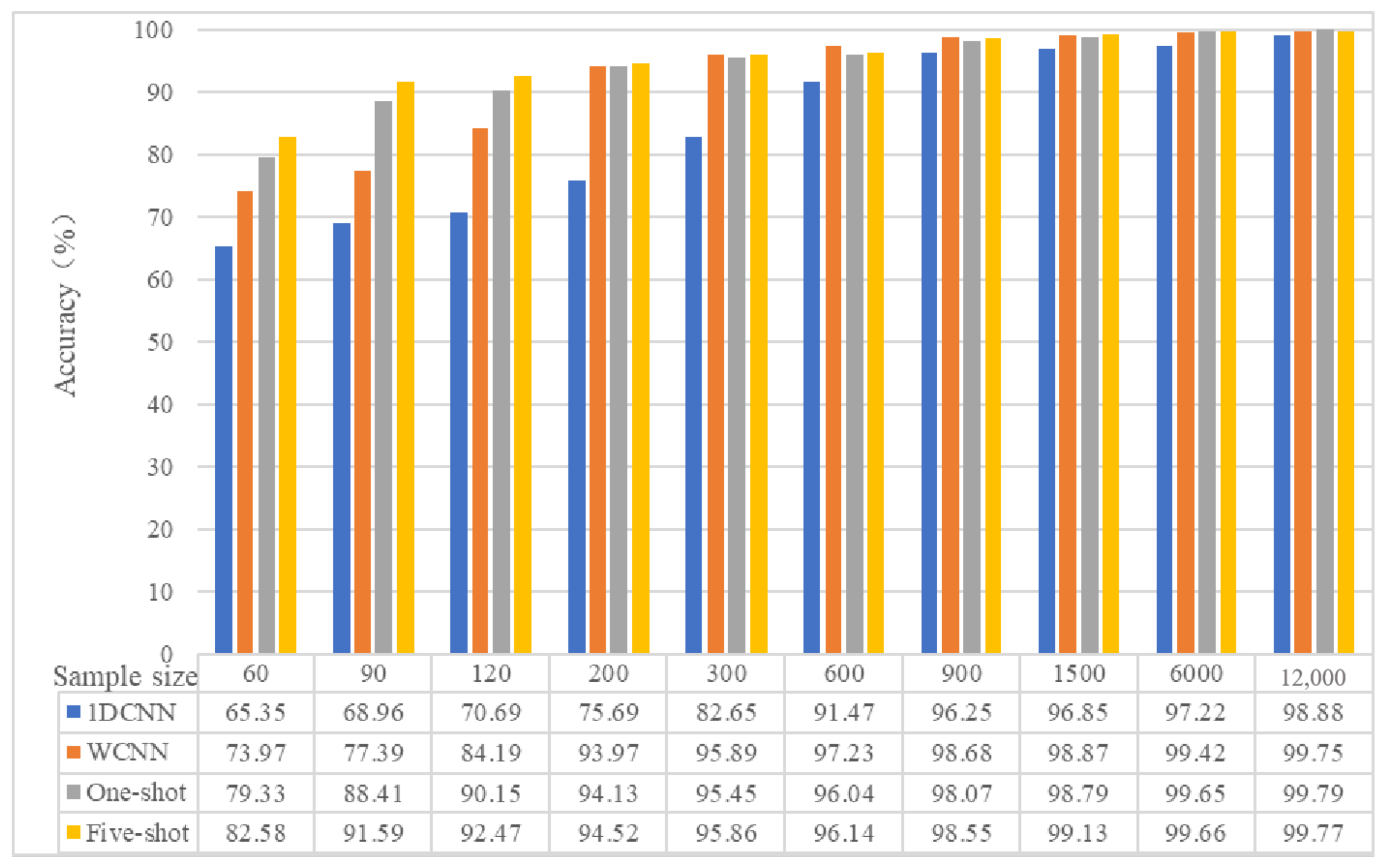
In order to verify the influence of training sample size on results, the test data set in data set D is taken as the test set, and 60, 90, 120, 200, 300, 600, 900, 1500, 6000, and 12,000 samples are randomly selected from the training samples of the whole data set D, and a series of comparative experiments are conducted. A total of 60% of the samples were used as the training set, and the remaining samples were used as the verification set to evaluate the influence of the number of samples on the performance of each training model. For each training set size, we repeated the sample selection process five times to generate five different training sets to handle the bias of randomly selected small training sets. For each such random training sample set, we repeated the algorithm training and test experiment four times to deal with the randomness of the algorithm, 20 times for each series of experiments. The experimental results are shown in Figure 4.

The following conclusions can be drawn from Figure 4:

• The accuracy of 1DCNN, WCNN, and few-shot learning increases with the increase of the number of training samples.
• The accuracy of five-shot learning is always higher than that of one-shot learning.

When the training samples are small (60, 90, 120) and large (300, 600, 900), the accuracy of the four methods is compared as shown in Figure 5.

The following conclusions can be drawn from Figure 5:

• When the number of training samples is small, the few-shot learning model performs better, and the average accuracy is 9% higher than that of the WCNN model. Especially when the training set size is set to 90, the accuracy of the few-shot learning model is 13% higher than that of the WCNN model.
• When the number of training samples is large, the accuracy of few-shot learning is slightly lower than that of WCNN, but both are higher than 94%. When the number of training samples increased to more than 900, the accuracy of the two algorithms was almost the same, higher than 98%.

In general, the few-shot learning algorithm proposed in this paper has better performance when training with limited data sets but has little advantage when training with rich samples.

3.3. Performance Comparison in Noisy Environment

In this experiment, the performance of the model under noise is discussed to simulate the variation of working conditions in data set D. The SNR (signal-to-noise ratio) is defined as the ratio of the strength of a signal to the strength of noise, usually expressed in decibels (dB).

The original data provided by CWRU were also used in the experiment to train the model. Here, only six representative training sample sizes (60, 90, 300, 1500, 6000, 12,000) were selected, and white Gaussian test samples with different SNR were added for testing. The SNR ranges from −4 db to 10 dB. The experimental results are shown in

Table 3. The accuracy of three models in noisy environments.

Model	Samp Size	SNR (dB)
		−4	−2	0	2	4	6	8	10	None
Five-shot	60	32.05	47.46	63.42	73.95	78.59	80.93	81.76	82.37	82.58
	90	34.70	50.15	66.53	79.93	86.44	89.69	90.58	91.25	91.59
	300	29.38	45.95	62.58	78.84	86.76	91.65	93.89	94.45	95.86
	1500	35.61	49.63	66.58	82.28	92.56	95.97	98.03	98.85	99.13
	6000	37.53	55.26	69.35	83.59	94.28	98.36	99.06	99.56	99.66
	12,000	41.25	57.85	71.38	85.59	95.12	98.93	99.57	99.70	99.77
One-shot	60	31.46	47.05	61.25	70.86	75.26	78.16	78.96	78.98	79.33
	90	33.65	48.79	65.36	78.59	84.69	86.36	87.89	88.31	88.41
	300	29.62	44.52	62.05	78.25	86.49	91.15	93.56	94.25	95.45
	1500	34.52	48.66	66.61	81.25	92.15	96.53	97.24	98.52	98.79
	6000	37.85	54.28	69.39	83.52	94.76	98.78	99.42	99.67	99.65
	12,000	41.26	57.45	71.35	85.75	95.16	98.59	99.62	99.73	99.79
WCNN	60	30.25	45.58	59.01	66.07	71.02	72.23	72.94	73.59	73.97
	90	39.88	56.39	67.59	71.48	74.41	75.74	76.58	77.54	77.39
	300	44.58	71.58	87.58	93.32	94.89	96.36	96.48	96.69	95.89
	1500	37.52	63.84	90.68	97.44	98.66	98.78	98.73	98.87	98.87
	6000	35.12	64.08	91.55	97.58	99.01	99.23	99.41	99.52	99.42
	12,000	45.06	63.63	83.39	94.91	98.91	99.55	99.62	99.71	99.75

.

As can be seen from the table, it is obvious that the accuracy rate will increase with the reduction of noise. For example, in 6000 training data samples, when the SNR is −4 dB, the average accuracy rate is only close to 40%, and when the SNR is 6 dB, the accuracy rate reaches the peak of more than 99%. When the noise is not very strong, the greater the amount of training data, the higher the accuracy.

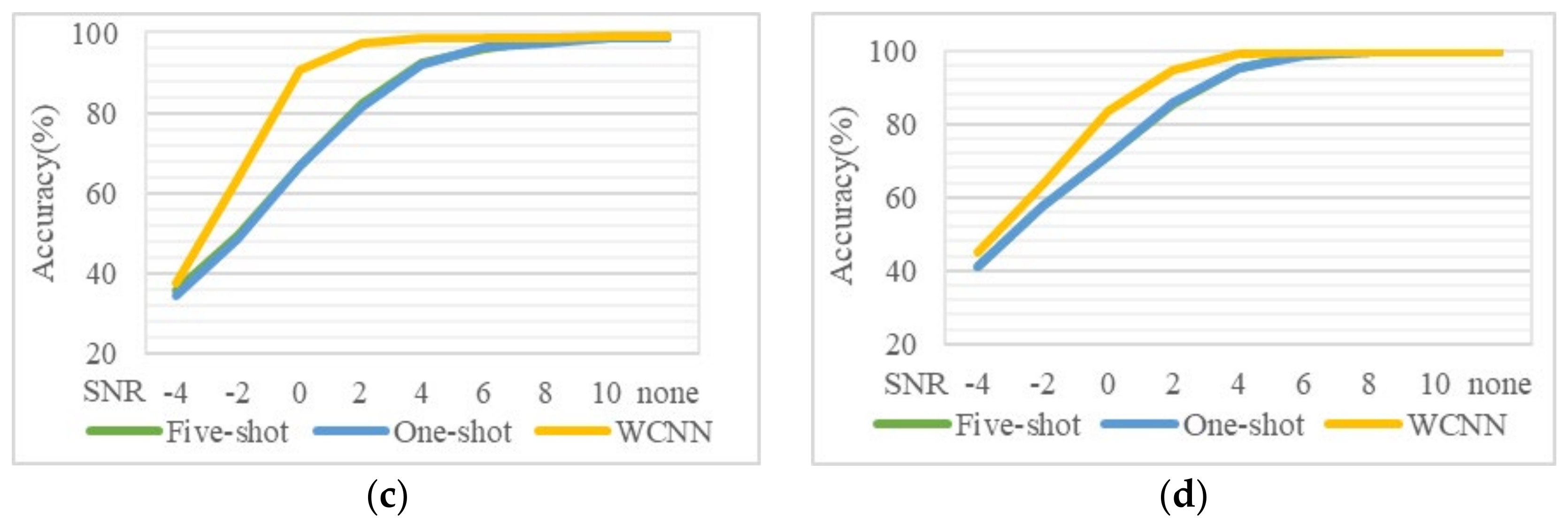
As shown in Figure 6, in order to test the effect of training sample size in a noisy environment, diagnostic results of four training samples of different sizes (60, 90, 1500, and 12,000) were compared.

From the results, it is easy to see that the accuracy of five-shot is generally higher than that of one-shot. For a small amount of training data, when the characteristics of the training set and the test set are similar, the performance of the few-shot learning is better than the WCNN algorithm. For example, in Figure 6b, when the SNR is −4 dB, the effect of few-shot learning is inferior to that of WCNN due to the large difference in features between the training set and the test set. When the SNR is 0 dB, the accuracy of few-shot learning is close to that of WCNN due to certain differences in the characteristics of the training set and the test set. However, when the SNR is 10 dB, the accuracy of few-shot learning is more than 10% higher than that of WCNN due to the similar characteristics of the training set and the test set. In addition, with sufficient training data, the accuracy of few-shot learning is almost always lower than that of WCNN.

In Figure 7, we compare the test results of the three models under different noise environments: In Figure 7a,b, the SNR is −4 dB and 0 dB, respectively. There is a big difference between the training set and the test set, and the performance of the model does not increase with the increase of the number of training samples. Because the training model is underfitting when the training sample is small, the accuracy will increase with the increase of the number of training samples. However, when the number of training samples increases and the difference between the training set and the test set is large, the model after training performs well in the training set but is prone to overfitting on the test set with large differences, resulting in lower accuracy. In Figure 7c,d, when the SNR is 4 dB and 8 dB, respectively, the difference between the training set and the test set is small. With the increase in the number of training samples, the diagnostic effect becomes better and better.

To sum up, as the number of training samples increases, test performance does not increase monotonically when there is a significant difference between test data set and training data set. Thus, an appropriate number of training samples can yield the best results on significantly different test sets.

4. Test Platform Design and Fault Diagnosis

Next, this paper designed a test platform for fault data collection. On this basis, current data of EMA under different degrees of interturn short circuit were collected, and the deep learning framework designed above was used for fault diagnosis. In the experiment, the model uses Adam as the optimizer, and the hyperparameters include kernel size, step size, batch size, number of iterations, activation function, batch normalization, etc. The computing resources used in the experimental part of this paper are an i7-11800HCPU and an RTX3060 graphics card, and the computing time is 5 s per epoch.

4.1. Modeling of PMSM

• $\left(a,b, c\right)$ coordinate system.

In natural coordinates, the stator voltage equation of PMSM is

$$U_{abc}=R_{abc}{I}_{abc}+{\displaystyle \frac{\mathrm{d}{\mathsf{\psi }}_{\mathrm{a}\mathrm{b}\mathrm{c}}}{\mathrm{d}\mathrm{t}}}$$

(4)

In the equation, $U_{abc}$ is the phase voltage of three-phase winding, $R_{abc}$ is the phase resistance of three-phase winding, $I_{abc}$ is the phase current of three-phase winding, and ${\mathsf{\psi }}_{\mathrm{a}\mathrm{b}\mathrm{c}}$ is flux distribution of permanent magnet material on three-phase winding in rotor.

In normal state, the three phases are symmetrical, each phase has the same self-inductance. Each phase has the same mutual inductance.

The electromagnetic torque equation is

$${\mathrm{T}}_{\mathrm{e}}={\displaystyle \frac{1}{2}}{\mathrm{p}}_{\mathrm{n}}\left({\mathrm{I}}_{\mathrm{a}\mathrm{b}\mathrm{c}}^{\mathrm{T}}{\mathsf{\psi }}_{\mathrm{a}\mathrm{b}\mathrm{c}}\right)$$

(5)

In the equation, ${\mathrm{T}}_{\mathrm{e}}$ is the electromagnetic torque of PMSM, ${\mathrm{p}}_{\mathrm{n}}$ is the polar number of PMSM.

The equation of mechanical motion is

$$J{\displaystyle \frac{\mathrm{d}{\omega }_m}{\mathrm{d}t}}={\mathrm{T}}_{\mathrm{e}}-T_L-B{\omega }_m$$

(6)

In the equation, $\mathrm{J}$ is the moment of inertia of PMSM, ${\mathsf{\omega }}_{\mathrm{m}}$ is the mechanical angular velocity of PMSM, ${\mathrm{T}}_{\mathrm{L}}$ is the load torque of PMSM, $\mathrm{B}$ is the damping coefficient of PMSM.

• $(\mathsf{\alpha },\mathsf{\beta })$ coordinate system.

Because the magnetomotive force in coordinate system $\left(\mathrm{a},\mathrm{b},\mathrm{c}\right)$ is equal to the total magnetomotive force in coordinate system $(\mathsf{\alpha },\mathsf{\beta })$, the projection of the magnetomotive force in coordinate system $\left(\mathrm{a},\mathrm{b},\mathrm{c}\right)$ is equal to that in coordinate system $(\mathsf{\alpha },\mathsf{\beta })$.

• $(\mathrm{d},\mathrm{q})$ coordinate system.

Similarly, according to the principle that the synthesized magnetomotive force in the coordinate system $(\mathrm{d},\mathrm{q})$ is equal to that in the coordinate system $(\mathsf{\alpha },\mathsf{\beta })$, then the projection of the magnetomotive force in the coordinate system $(\mathrm{d},\mathrm{q})$ is equal to that in the coordinate system $(\mathsf{\alpha },\mathsf{\beta })$.

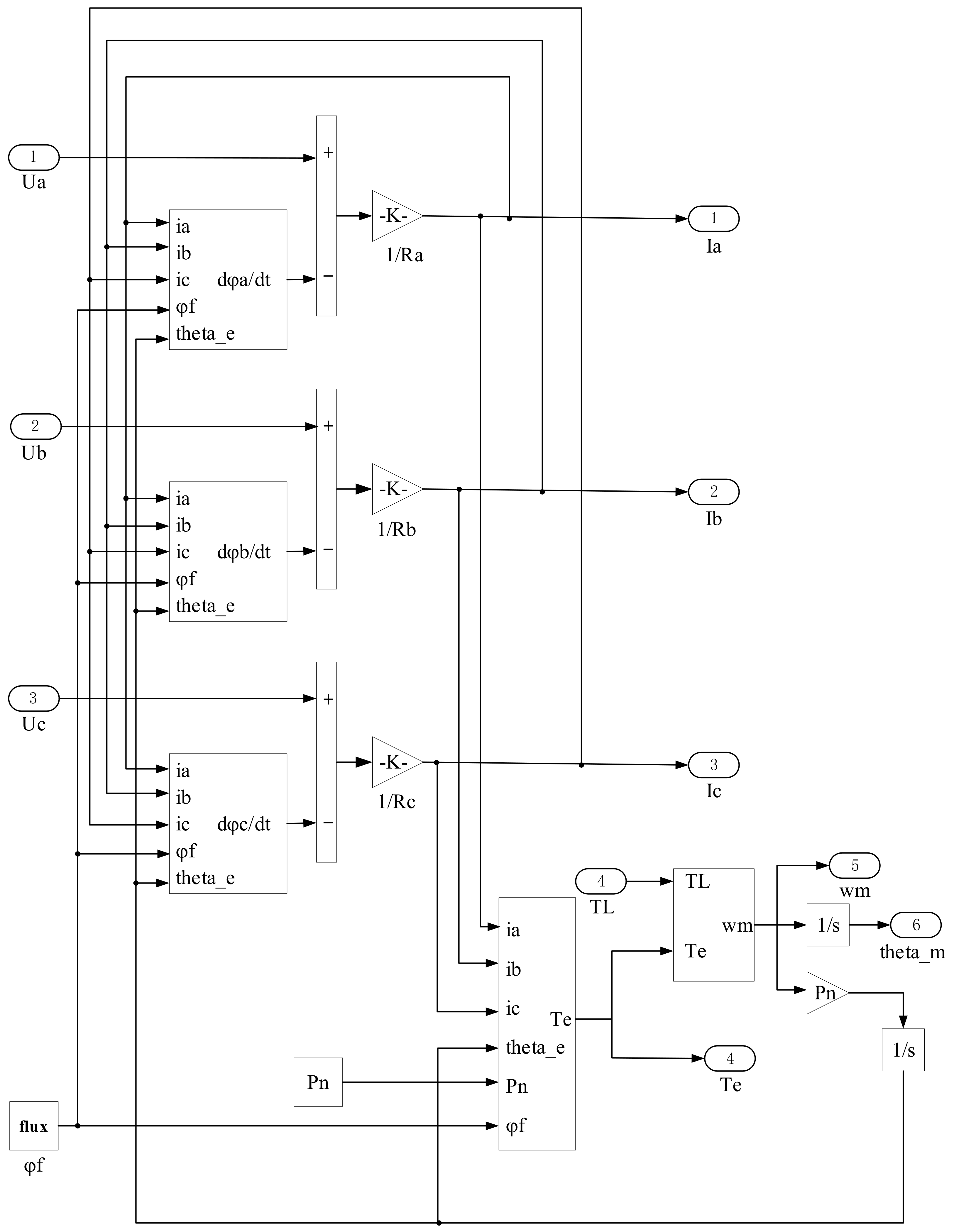
Based on the mathematical model of PMSM in a natural coordinate system, it is modeled and simulated in MATLAB/Simulink. The normal PMSM model is built according to the mathematical model of PMSM in the coordinate system $(\mathrm{a},\mathrm{b},\mathrm{c})$ mentioned above. The normal PMSM model contains four input signals and six output signals. The input signal mainly includes three-phase voltage and load torque, and the output signal includes three-phase current, electromagnetic torque, motor speed, and angle. The main parameters involved in the model are moment of inertia, pole-pair number, phase self-inductance, mutual inductance, a-phase resistance, b-phase resistance, c-phase resistance, friction coefficient, and permanent magnet flux linkage [26,27,28,29]. Figure 8 shows the internal structure of the model.

4.2. Interturn Short Circuit Fault Model of PMSM

The short-circuit model between turns of PMSM can be established. Based on the PMSM normal model, an input signal $\mathsf{\sigma }$, is added to the PMSM short-circuit model, representing the short-circuit proportion between turns of the motor [30,31].

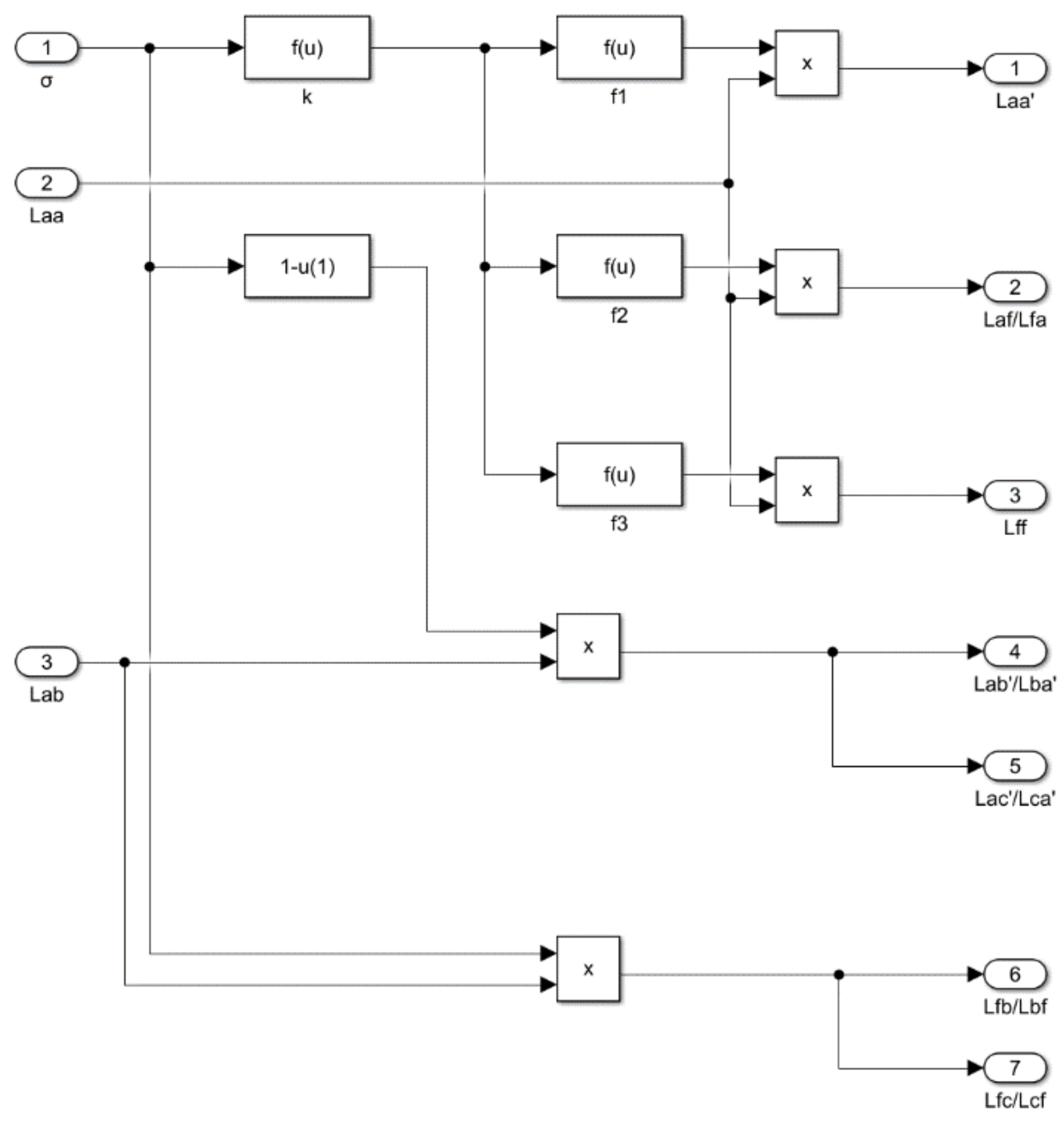
The key component of the PMSM short-circuit model is the inductance parameter calculation module established. Figure 9 shows the internal structure. The PMSM short-circuit model is based on the PMSM normal model.

4.3. Simulation Result Analysis

In order to find the appropriate fault parameters, the closed-loop control model of EMA is established. The control of EMA is essentially a closed-loop control of the internal motor. In this simulation modeling, it is assumed that the internal motor is a surface-mounted permanent magnet synchronous motor, and the most common Id = 0 control is used to establish a current-speed-position three closed-loop control system. Through the calculation and analysis of the simulation results, we obtain the results as shown in

Table 4. The change of signals after a fault occurs.

Signal	Degree of Change
	1% Short Circuit	5% Short Circuit	10% Short Circuit
Linear velocity	+1%	+1%	+1%
Linear displacement	0	0	0
Current of a-phase	+9%	+25%	+47%
Current of b-phase	+5%	+16%	+33%
Current of c-phase	−7%	−20%	−35%
Force	−14~+14%	−32~32%	−51~51%

.

When an interturn short-circuit fault occurs in the motor in EMA, the three-phase current of the motor will no longer be symmetrical, and the degree of asymmetry will gradually deepen with the increase of short-circuit degree. The output force and output linear velocity of EMA fluctuated, and the fluctuation amplitude increased gradually with the increase of short-circuit degree. The linear displacement of EMA’s output is basically unchanged. Although the output force fluctuates obviously, there are many factors causing the force fluctuation, such as electrical and mechanical faults of the motor and other EMA components. Although the output linear velocity fluctuates, the fluctuation range is too small, and it is easy to be drowned by noise in practice. The output linear displacement is basically unaffected by the interturn short circuit. In summary, three-phase current is selected as the characteristic quantity of subsequent fault diagnosis.

4.4. Test Platform Design

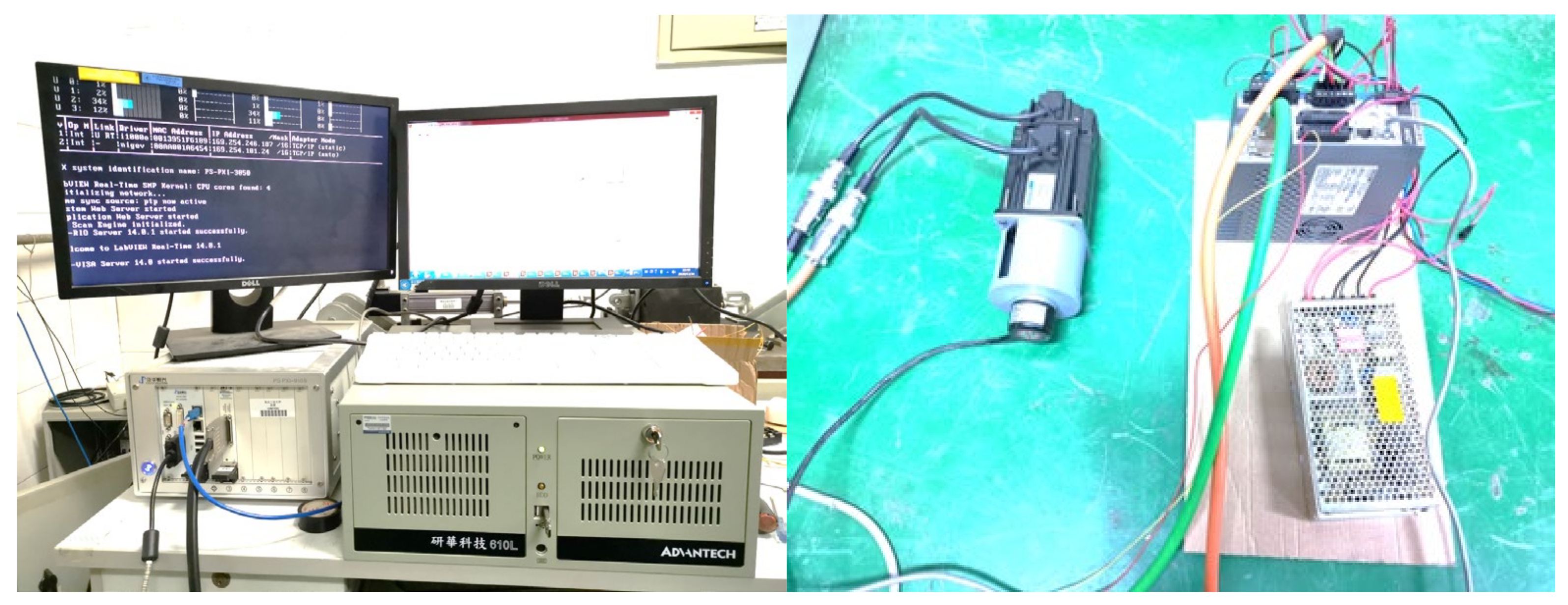
The fault test platform is mainly composed of the following parts: EMA, control device, signal acquisition device, fault simulation device, etc. As shown in Figure 10 [32].

The control unit is responsible for driving the EMA and providing position instructions for the EMA; the fault simulator is responsible for adding faults to the EMA; the loading device is responsible for providing loads for the EMA to simulate the actual working conditions; and the signal acquisition device is responsible for collecting various data during the operation of the EMA and transmitting control-related parameters to the control unit to realize closed-loop control.

The three-phase windings of the motor are externally connected. Two phase windings are connected with a resistance of the same resistance value, and the other phase is connected with a resistance of a different resistance value to simulate the asymmetry of the three-phase windings. At the same time, the three-phase current and speed signals of the motor under different fault depths are collected.

4.5. Fault Data Acquisition

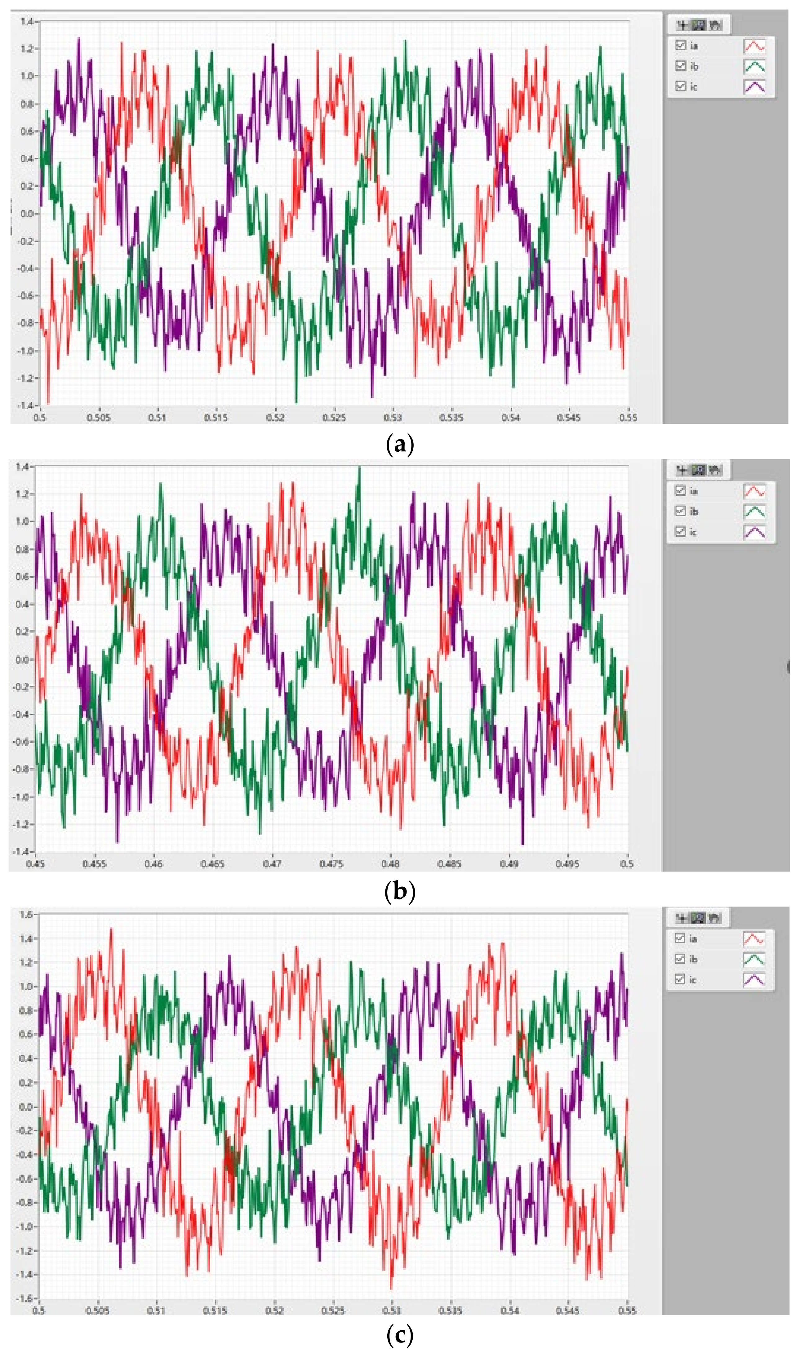
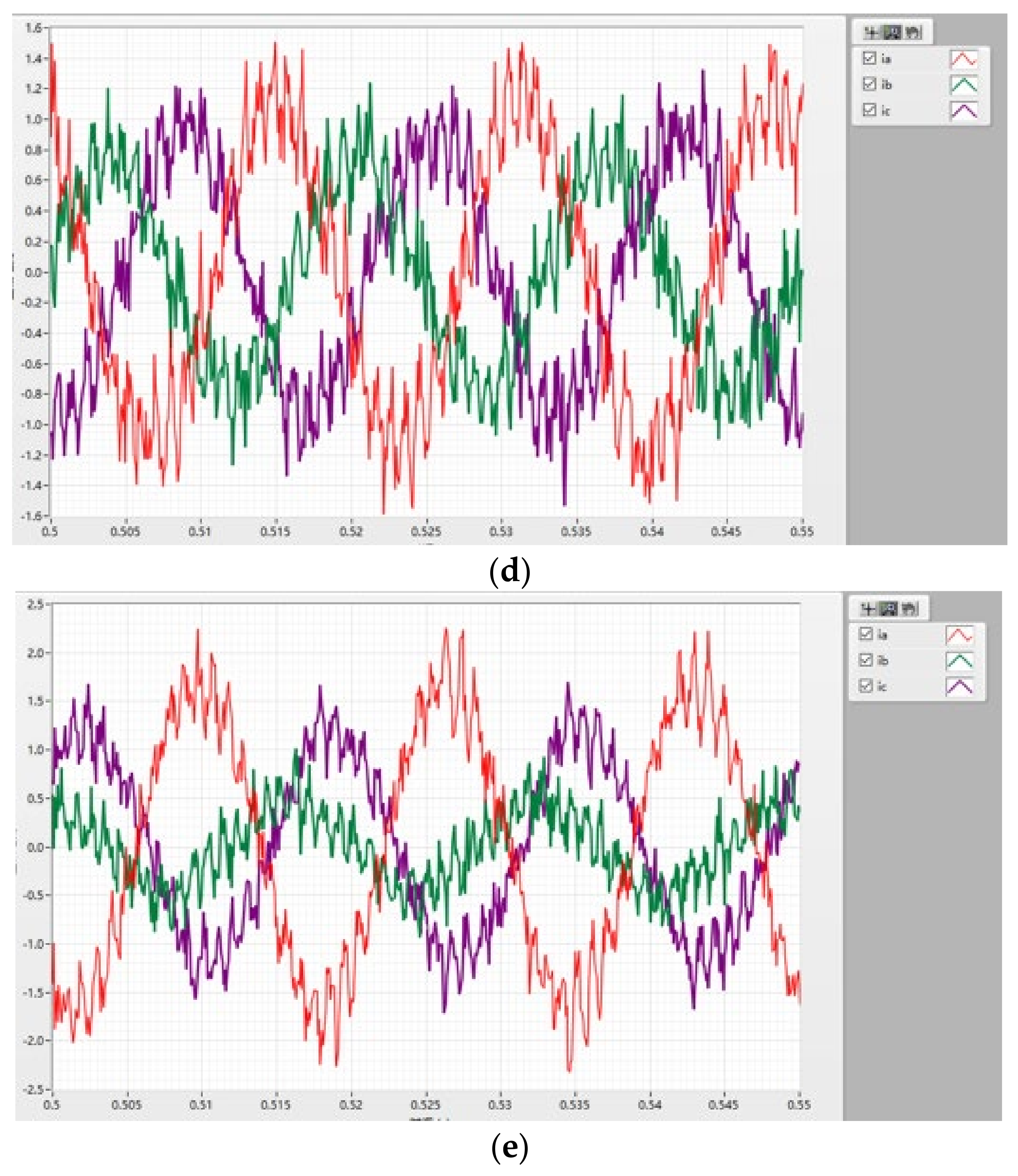
We connected all three phases of the circuit in series with resistors of the same size to simulate EMA under normal working conditions. Then, we removed the resistors of phase-A in series step by step to simulate different degrees of inter-turn short circuit and collected the three-phase current data under each state. Three-phase current signals in five states can be obtained as shown in Figure 11.

In Figure 11, the red curve represents the A phase, the green curve represents the B phase, and the purple curve represents the C phase. Combined with the above, the red curve representing the A phase represents the short-circuit phase current.

In this part, we connected all three phases of the circuit in series with resistors of the same size to simulate EMA under normal working conditions. Then, we removed the resistors of phase-A in series step by step to simulate different degrees of inter-turn short circuit and collected the three-phase current data under each state. These five different states are represented by (a) normal; (b) slight; (c) mild; (d) moderate; and (e) heavy.

4.6. Fault Diagnosis

The sampled three-phase current data contain three-phase current data in five states. A total of 200 groups of data in each state are selected as the training set and 50 groups as the test set, as shown in

Table 5. Description of three-phase current data.

Fault State	Phase	Training Set/Test Set	Label
Normal	\	200/50	0
Slight	A	200/50	1
	B	200/50	2
	C	200/50	3
Mild	A	200/50	4
	B	200/50	5
	C	200/50	6
Moderate	A	200/50	7
	B	200/50	8
	C	200/50	9
Heavy	A	200/50	10
	B	200/50	11
	C	200/50	12

.

According to the method similar to Section 4, the training data sets of all groups were taken as the test set, and 60, 90, 120, 200, 300, 500, 800, and 1000 samples were randomly selected from the training samples of the whole data set to conduct a series of comparative experiments. A total of 60% of the samples were used as the training set, and the remaining samples were used as the verification set to evaluate the influence of the number of samples on the performance of each training model. For each training set size, we repeated the sample selection process five times to generate five different training sets to handle the bias of randomly selected small training sets. For each such random training sample set, we repeated the algorithm training and test experiment four times to deal with the randomness of the algorithm, 20 times for each series of experiments. The experimental results are shown in

Table 6. Model accuracy under different training samples.

	Sample	60	90	120	200	300	500	800	1000
Model
1DCNN		59.27	62.57	65.41	71.29	80.06	89.58	92.47	94.35
WCNN		70.56	76.92	82.53	88.59	93.82	95.61	96.19	96.54
One-shot		75.64	85.49	88.92	92.85	93.94	94.15	95.25	96.01
Five-shot		81.67	88.95	90.76	92.36	94.42	95.04	95.33	96.26

.

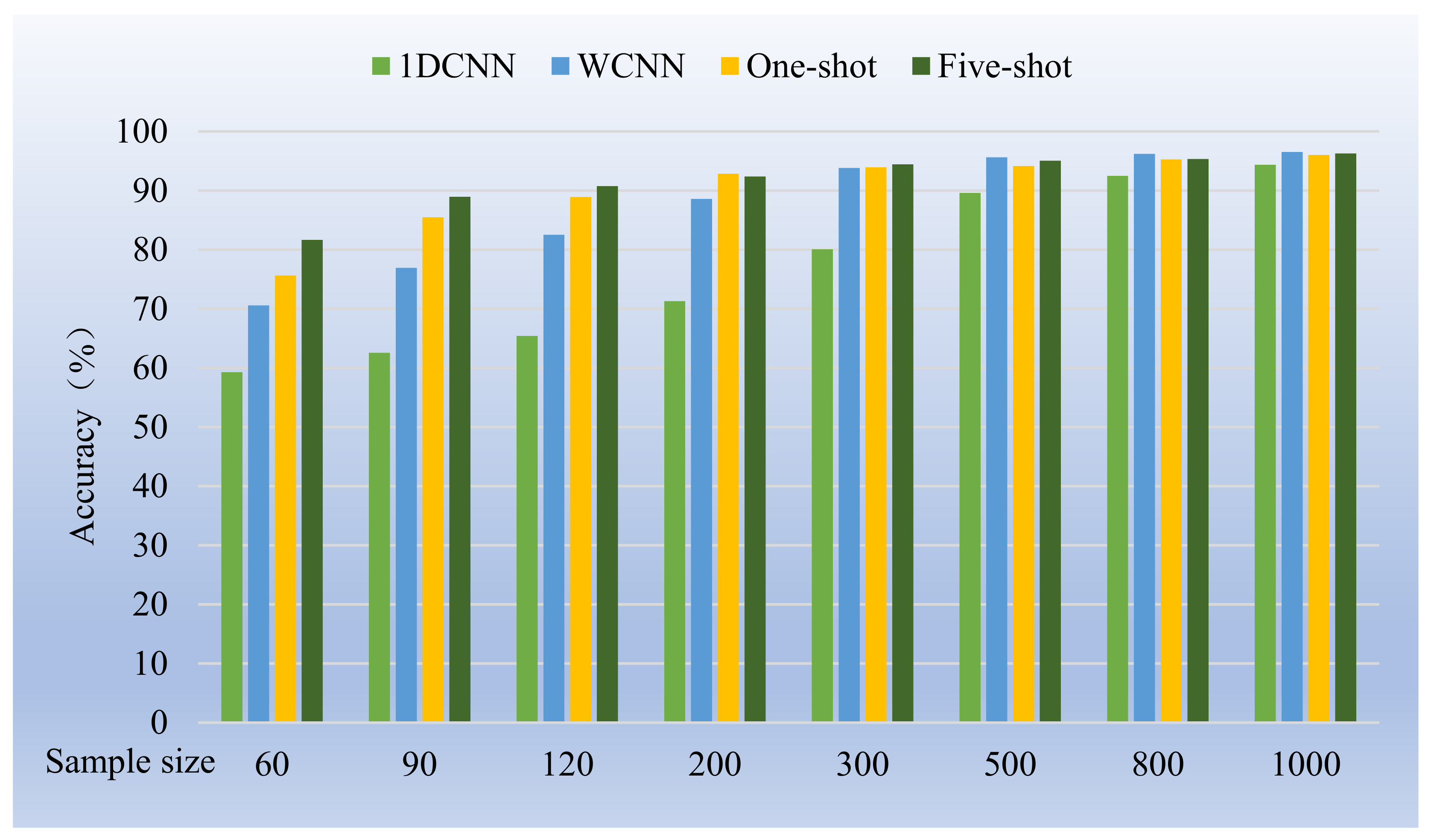
It can be seen from the table that, under the same samples, the accuracy of several models is basically reduced compared with that in Section 4. The reason should be that the data collected in this chapter are of lower quality compared with the fault data set used in Section 4. In order to analyze the accuracy of each model under different samples, the data in Table 6 are converted into bar charts for observation, as shown in Figure 12.

Figure 12 shows the following:

• The accuracy of 1DCNN, WCNN, and few-shot learning increased with the increase of the number of training samples.
• The accuracy of WCNN is basically higher than that of 1DCNN; the accuracy of five-shot learning is basically higher than that of one-shot learning.

Figure 13, respectively, shows the comparison of accuracy when the training samples are small (60, 90, and 120) and large (500, 800, and 1000).

Figure 13, respectively, shows the comparison of accuracy when the training samples are small (60, 90, and 120) and large (500, 800, and 1000). As can be seen from the figure:

• When the training sample is small, the performance of the algorithm of few-shot learning is better than that of WCNN and 1DCNN. The average accuracy of the few-shot learning model is about 8% higher than that of the WCNN model. Especially when the training set size is 90, the accuracy of the few-shot learning model is about 10% higher than that of the WCNN model.
• When the training sample is large, the performance of the model of few-shot learning is slightly worse than that of WCNN, but the accuracy of the two algorithms is actually very close, only about 1% difference. When the number of training samples increased to 1000, the performance of two algorithms are almost the same, and the accuracy rate was higher than 96%.

In general, the small sample learning algorithm proposed in this paper has higher accuracy when training with limited data sets, and the improvement effect is significant, which has strong engineering application value.

5. Conclusions

In recent years, with the continuous development of science and technology in the world, artificial intelligence has been more and more widely used. Intelligent diagnosis has also become the mainstream in the field of fault diagnosis by virtue of its ability to analyze large amounts of data and automatically generate diagnostic results. Compared with traditional machine learning, deep learning has a stronger feature extraction ability and has a wide range of applicability and model migration capabilities. It has become a new star in the field of intelligent diagnosis and has been applied to all walks of life.

The fault diagnosis method based on deep learning can diagnose the fault of the equipment quickly and accurately, but it requires a lot of data when training the model. In the development and testing stage of the equipment, it is difficult to find a large amount of data to train the model. Therefore, when the fault sample is not enough to complete the training of the model, a method that can still effectively complete the fault diagnosis under a small sample is needed.

This paper studied the fault diagnosis method of PMSM, the core component of EMA. Firstly, Simulink was used to model EMA components, and the interturn short-circuit fault with high hazards was simulated. By observing the changes of EMA signals after the short-circuit fault occurred, the current signal of the three-phase circuit was selected as the characteristic signal.

Firstly, based on the classical convolutional neural network, according to the characteristics of one-dimensional signals, WCNN is formed by improving the size of the convolution kernel. At the same time, aiming at the problem of small fault samples under actual working conditions, the twin neural network is introduced, and the two are combined to form a small sample learning model. Through experiments, the accuracy of each model under different training samples and different SNR environments is compared. It can be concluded that under the condition of small samples, the accuracy of the proposed method is 8% higher than that of WCNN on average, and it has certain anti-noise performance.

Then, in view of the shortcoming that it is difficult to find a large amount of data to train the model in the research and development stage of the equipment, a fault diagnosis method that can still achieve high accuracy in the case of small fault samples is needed. In this paper, we design a deep learning framework that only needs a small amount of fault data to complete the fault diagnosis and can achieve high accuracy, and we use the general data set to verify the effectiveness of the method.

Finally, the EMA fault test platform was built, and the method of external resistance was used to simulate the interturn short circuit fault of PMSM, and the three-phase current data under different fault degrees were collected, and the collected data were used to complete the fault diagnosis of PMSM. The experimental results show that the accuracy of the deep learning framework designed in this paper increases by 8% on average compared with WCNN under the condition of limited data, which has good engineering value.

The limitations of this study lie in the following aspects: Only the inter-turn short circuit fault of the permanent magnet synchronous motor in EMA is studied, and the remaining faults of EMA can be further studied. Only the research of fault diagnosis is carried out. In the actual working conditions, further fault prediction can have greater practical value. In the fault simulation, only the change of internal resistance under an inter-turn short circuit is considered, and the influence of inductance and other parameters is ignored, so that the quality of the collected fault signal is not high enough, and the fault simulation device needs to be further improved.

References

- Jean-Charles, M.A.R.É.; Jian, F.U. Review on signal-by-wire and power-by-wire actuation for more electric aircraft. Chin. J. Aeronaut. 2017, 30, 857–870. [Google Scholar]
- Huang, W.W.; Zhu, Z.; Zhang, X.; Zhu, L.M. A hybrid electromagnetic-piezoelectric actuated tri-axial fast tool servo integrated with a three-dimensional elliptical vibration generator. Precis. Eng. 2024, 86, 213–224. [Google Scholar] [CrossRef]
- Bae, S.J.; Lee, S.J.; Joo, M.G. Dual magnet solenoid actuator: Practical applications. Sens. Actuators A Phys. 2024, 365, 114893. [Google Scholar] [CrossRef]
- Qiao, G.; Liu, G.; Shi, Z.; Wang, Y.; Ma, S.; Lim, T.C. A review of electromechanical actuators for more/all electric aircraft systems. Proc. Inst. Mech. Engineer. Part C J. Mech. Eng. Sci. 2018, 232, 4128–4151. [Google Scholar] [CrossRef]
- Fu, J.; Maré, J.C.; Fu, Y. Modelling and simulation of flight control electro mechanical actuators with special focus on model architecting, multidisciplinary effects and power flows. Chin. J. Aeronaut. 2017, 30, 47–65. [Google Scholar] [CrossRef]
- Qi, R.; Wang, L.; Zhou, X.; Xue, J.; Jin, J.; Yuan, L.; Shen, Z.; Deng, G. Embedded piezoelectric actuation method for enhanced solar wings vibration control. Int. J. Mech. Sci. 2024, 274, 109271. [Google Scholar] [CrossRef]
- Qu, S.; Zappaterra, F.; Vacca, A.; Busquets, E. An electrified boom actuation system with energy regeneration capability driven by a novel electro-hydraulic unit. Energy Convers. Manag. 2023, 293, 117443. [Google Scholar] [CrossRef]
- Qiao, S.; Hao, Y.; Quan, L.; Ge, L.; Xia, L. Design and Analysis of a Novel Impact—Resistant Electro-Mechanical Actuator with Disc Spring Compression and Hydraulic Buffering Mechanism. IEEE/ASME Trans. Mechatron. 2024, 29, 2138–2149. [Google Scholar] [CrossRef]
- Liu, Z.; Yu, T.; Hong, R.; Liu, L.; Su, H.; Lin, J.; Jiang, C.; Shang, Y. Analysis of Electro-mechanical Actuator Transmission Clearance under High-temperature Conditions. In Proceedings of the 2023 9th International Conference on Fluid Power and Mechatronics, Lanzhou, China, 18–21 August 2023; FPM: Dorset, UK, 2023. [Google Scholar]
- Kang, J.G.; Kwon, J.Y.; Lee, M.S. A Dynamic Power Consumption Estimation Method of Electro-mechanical Actuator for UAV Modeling and Simulation. Int. J. Aeronaut. Space Sci. 2022, 23, 233–239. [Google Scholar] [CrossRef]
- Ismail, M.A.A.; Balaban, E.; Spangenberg, H. Fault detection and classification for flight control electromechanical actuators. In Proceedings of the IEEE Aerospace Conference, Big Sky, MT, USA, 5–12 March 2016; pp. 1–10. [Google Scholar]
- Huang, W.; Huang, Y.; Luo, L.; Zhou, L. A Mixed Logical Dynamic Model-Based Open-Circuit Fault Diagnosis Method for Five-Phase PMSM Drives. In Proceedings of the 2023 26th International Conference on Electrical Machines and Systems, Zhuhai, China, 5–8 November 2023; pp. 3641–3646. [Google Scholar]
- Honglin, L.; Li, F.; Rui, Y.; Shuiqing, X.; Kenan, D. Inverter and Sensor Fault Diagnosis of PMSM Drive System Based on Improved WOA-LSTM; Lecture Notes in Electrical Engineering, 1161 LNEE; Springer: Berlin/Heidelberg, Germany, 2024; pp. 471–478. [Google Scholar]
- Dai, Y.; Zhang, L.; Xu, D.; Chen, Q.; Li, J. Development of Deep Learning-Based Cooperative Fault Diagnosis Method for Multi-PMSM Drive System in 4WID-EVs. IEEE Trans. Instrum. Meas. 2024, 73, 3506513. [Google Scholar] [CrossRef]
- Ferreira, R.S.; Ferreira, A.C. Investigation of cable influence on the interturn transient voltage distribution in rotating machine windings using a three-phase model. Electr. Power Syst. Res. 2021, 196, 107291. [Google Scholar] [CrossRef]
- Li, J.; Liu, J.; Chen, Y. A fault warning for inter-turn short circuit of excitation winding of synchronous generator based on GRU-CNN. Glob. Energy Interconnect. 2022, 5, 236–248. [Google Scholar] [CrossRef]
- Hosny, K.M.; Magdi, A.; ElKomy, O.; Hamza, H.M. Digital image watermarking using deep learning: A survey. Comput. Sci. Rev. 2024, 53, 100662. [Google Scholar] [CrossRef]
- Liu, F.; Li, W.; Wu, Y.; He, Y.; Li, T. Fault Diagnosis of Imbalance and Misalignment in Rotor-Bearing Systems Using Deep Learning. Pol. Marit. Res. 2024, 31, 102–113. [Google Scholar] [CrossRef]
- An, Z.; Wu, F.; Zhang, C.; Ma, J.; Sun, B.; Tang, B.; Liu, Y. Deep Learning-Based Composite Fault Diagnosis. IEEE J. Emerg. Sel. Top. Circuits Syst. 2023, 13, 572–581. [Google Scholar] [CrossRef]
- Wang, A.; Ge, Y. Research on convolutional neural networks in motor fault diagnosis. In Proceedings of the SPIE—The International Society for Optical Engineering, Guilin, China, 20–22 October 2023; Volume 13082. [Google Scholar]
- Yang, X.; Bi, F.; Cheng, J.; Tang, D.; Shen, P.; Bi, X. A Multiple Attention Convolutional Neural Networks for Diesel Engine Fault Diagnosis. Sensors 2024, 24, 2708. [Google Scholar] [CrossRef]
- Xu, J.-H.; Zhang, B.-X.; Zhu, K.-Q.; Zheng, X.-Y.; Zhang, C.-L.; Chen, Z.-L.; Yang, Y.-R.; Huang, T.-M.; Bo, Z.; Wan, Z.-M.; et al. Fault diagnosis of PEMFC based on fatal and recoverable failures using multi-scale convolutional neural networks. Int. J. Hydrogen Energy 2024, 80, 916–925. [Google Scholar] [CrossRef]
- Cheng, L.; An, Z.; Guo, Y.; Ren, M.; Yang, Z.; Mcloone, S. MMFSL: A Novel Multimodal Few-Shot Learning Framework for Fault Diagnosis of Industrial Bearings. IEEE Trans. Instrum. Meas. 2023, 72, 3525313. [Google Scholar] [CrossRef]
- Tam, S.; Boukadoum, M.; Campeau-Lecours, A.; Gosselin, B. Siamese Convolutional Neural Network and Few-Shot Learning for Embedded Gesture Recognition. In Proceedings of the 20th IEEE International Interregional NEWCAS Conference, NEWCAS 2022—Proceedings, Quebec City, QC, Canada 19–22 June 2022; pp. 114–118. [Google Scholar]
- Zheng, L.; Liu, M.; Zhang, S.; Liu, Z.; Dong, S. End-to-end multi-sensor fusion method based on deep reinforcement learning in UASNs. Ocean. Eng. 2024, 305, 117904. [Google Scholar] [CrossRef]
- Li, D.; Chen, J.; Xie, R.; Luo, Z.; Sheng, Y.; Hu, M.; Wang, G.; Zhang, M. A Novel Frequency Estimation Strategy and Filter Based on the Gearbox Response Mechanism Model. SSRN 2024, 30, 2003619. [Google Scholar]
- Hara, T.; Taniguchi, S.; Ajima, T.; Sawahata, M.; Hori, M.; Tsukagoshi, T.; Hoshino, K. Synchronous PWM Control with Carrier Wave Phase Shifts for Permanent Magnet Synchronous Motor. IEEE Trans. Ind. Appl. 2022, 58, 5650–5658. [Google Scholar] [CrossRef]
- Hara, T.; Tsukagoshi, T.; Taniguchi, S.; Ajima, T. Vibration Reduction of Permanent Magnet Synchronous Motor Driven by Synchronous PWM Control with Carrier Wave Phase Shifts. IEEJ J. Ind. Appl. 2022, 11, 379–387. [Google Scholar] [CrossRef]
- Sheshadri, V.; Mishra, R.K.; Kamath, R. Performance Analysis of Various PWM Strategies for Control of Permanent Magnet Synchronous Machines in High Voltage EV Application. In Proceedings of the ITEC-India 2023—5th International Transportation Electrification Conference: eAMRIT—Accelerating e-Mobility Revolution for India’s Transportation, Chennai, India, 12–15 December 2023. [Google Scholar]
- Bastard, P.; Bertrand, P.; Meunier, M. A transformer model for winding fault studies. IEEE Trans. Power Deliv. 2002, 9, 690–699. [Google Scholar] [CrossRef]
- Wang, X.; Liu, G.; Chen, Q.; Farahat, A.; Song, X. Multivectors Model Predictive Control with Voltage Error Tracking for Five-Phase PMSM Short-Circuit Fault-Tolerant Operation. IEEE Trans. Transp. Electrif. 2022, 8, 675–687. [Google Scholar] [CrossRef]
- Zhang, C.; Huang, Q.; Zhang, C.; Yang, K.; Cheng, L.; Li, Z. ECNN: Intelligent Fault Diagnosis Method Using Efficient Convolutional Neural Network. Actuators 2022, 11, 275. [Google Scholar] [CrossRef]
Figure 1.
Structure of WCNN.
Figure 2.
The general strategy of few-shot learning.