Optimization Design of a Polyimide High-Pressure Mixer Based on SSA-CNN-LSTM-WOA

Abstract

Foam mixers are classified as low-pressure and high-pressure types. Low-pressure mixers rely on agitator rotation, facing cleaning challenges and complex designs. High-pressure mixers are simple and require no cleaning but struggle with uneven mixing for high-viscosity substances. Traditionally, increasing the working pressure resolved this, but material quality limits it at higher pressures. To address the issues faced by high-pressure mixers when handling high-viscosity materials and to further improve the mixing performance of the mixer, this study focuses on a polyimide high-pressure mixer, identifying four design variables: impingement angle, inlet and outlet diameters, and impingement pressure. Using a Full Factorial Design of Experiments (DOE), the study investigates the impacts of these variables on mixing unevenness. Sample points were generated using Optimal Latin Hypercube Sampling—OLH. Combining the Sparrow Search Algorithm (SSA), Convolutional Neural Network (CNN), and Long Short-Term Memory Network (LSTM), the SSA-CNN-LSTM model was constructed for predictive analysis. The Whale Optimization Algorithm (WOA) optimized the model, to find an optimal design variable combination. The Computational Fluid Dynamics (CFD) simulation results indicate a 70% reduction in mixing unevenness through algorithmic optimization, significantly improving the mixer’s performance.

1. Introduction

Polyimide foam is considered one of the most versatile high-performance materials of the new century, with excellent mechanical properties, dielectric properties, organic solvent resistance, high-temperature resistance, and radiation resistance. Due to these exceptional properties, its demand is increasing in fields such as engineering materials processing, microelectronics, aerospace, and the military [1]. Currently, polyimide foaming machines are adapted from polyurethane foaming machines, leading to discrepancies between the two materials. In actual production, the uneven mixing of raw materials can result in the poor quality of the final molded products, low yield rates, and an inability to meet market demands. To improve the material’s evenness, the most important component mixer should be sufficiently considered and designed.

The mixer is the core component of the polyimide foaming machine, and its performance directly affects the quality of the foam. To address the issue of uneven mixing in the mixer, in addition to altering the operating parameters of the mixing head during the mixing process [2], research on the optimization of the mixing head structure has demonstrated that parameters such as the impingement angle, inlet diameter, outlet diameter, and pressure all influence the mixing effect of the mixer [3,4]. Yuan Xiaohui et al. [5] used the software “Ansys” (ANSYS 2022r1) to analyze the flow field of materials in the mixer’s foaming machine, focusing on the unfolded flow channel. The shear stress was then determined based on the velocity field, revealing that circulation in the cross-sectional direction promotes the thorough mixing of materials in the foaming machine. Trautmann et al. [6] conducted experimental research on the impingement angle and found that it influences the mixing effect of the mixing head. Guo et al. [7] analyzed the mixing mechanism of the foaming machine, confirming that high-pressure impingement mixing is superior to low-pressure mixing. They also analyzed factors affecting the mixing effect, such as the impingement pressure and feed diameter. Schneider [8] and Bayer [9] designed a feed port with an asymmetric structure, where the fluid inlet is designed as a high-pressure nozzle. Their research suggested that high-pressure mixing achieves a more uniform blend compared to low-pressure mixing. Murphy et al. [10] conducted a detailed study of the factors affecting rapid liquid–liquid mixing in impingement stream mixers, providing a theoretical basis for the optimization design of mixers. Van Horn et al. [11] designed flow channels in a Venturi shape, utilizing a reduction in diameter to increase the flow velocity of the two fluid streams.

There are various optimization methods for fluid machinery, including traditional verification methods and intelligent optimization techniques [12,13]. The former relies on extensive data and experience, while the latter employs approximate models such as the response surface method, kriging models, and artificial neural networks, utilizing intelligent algorithms like genetic algorithms and particle swarm optimization for the optimization process. Luo et al. [14] established a predictive model of centrifugal pump parameters using a backpropagation (BP) neural network and then sought the optimum value using genetic algorithms. After optimization, the impeller efficiency increased by 1.4%. Jiang et al. [15] utilized the orthogonal experimental method to analyze the impact of design parameters on mixing efficiency, and then applied the GA-BP-GA methodology for the structural optimization of the mixer. Following optimization, the mixing index decreased by 52%. Li et al. [16] employed the response surface method to create a regression predictive model for supersonic nozzles, and using genetic algorithms, determined the optimal structural parameters for the nozzle. Compared to traditional optimization methods, the approach that combines approximate models with intelligent algorithms for fluid machinery optimization can effectively enhance the efficiency of the optimization process and reduce the time cycle.

In summary, to address the issue of uneven mixing in polyimide mixers handling high-viscosity liquids, we focused on the impact of the mixing head’s structure on its performance. Both domestic and international studies primarily employ fluid simulation techniques to visualize flow fields, optimizing structures and operational parameters based on the mixer’s performance [17,18,19]. Building on the existing high-pressure foam equipment of a particular company, we assessed the impact of each structural component on mixing unevenness using full factorial DOE and factor analysis. Samples were extracted through OLH, and predictive models of mixing unevenness were established using the SSA-CNN-LSTM. Subsequently, the WOA was used to optimize structural parameters, aiming to enhance the mixing efficiency and structure of the mixing head.

2. CFD Simulation of Three-Phase Fluid Flow in a Polyimide Mixer

A high-pressure polyimide mixer is essential for producing polyimide foams. The research, development, and design of such equipment often rely on empirical formulas, leading to high uncertainty and lengthy development cycles. In some experiments, techniques like Planar Laser-Induced Fluorescence (PLIF) and Particle Image Velocimetry (PIV) visualize fluid concentration and velocity within the flow field [20,21]. For mixers synthesized from reactants, methods such as Transmission Electron Microscopy (TEM) and wavelength dispersive X-ray fluorescence spectroscopy accurately characterize nanoparticle composition and size distribution [22,23]. However, experimental research methodologies require significant time and resources. This chapter will treat the mixer as a black box, using CFD simulation techniques to visually investigate the polyimide high-pressure mixer.

2.1. Mixed Head Structure Analysis

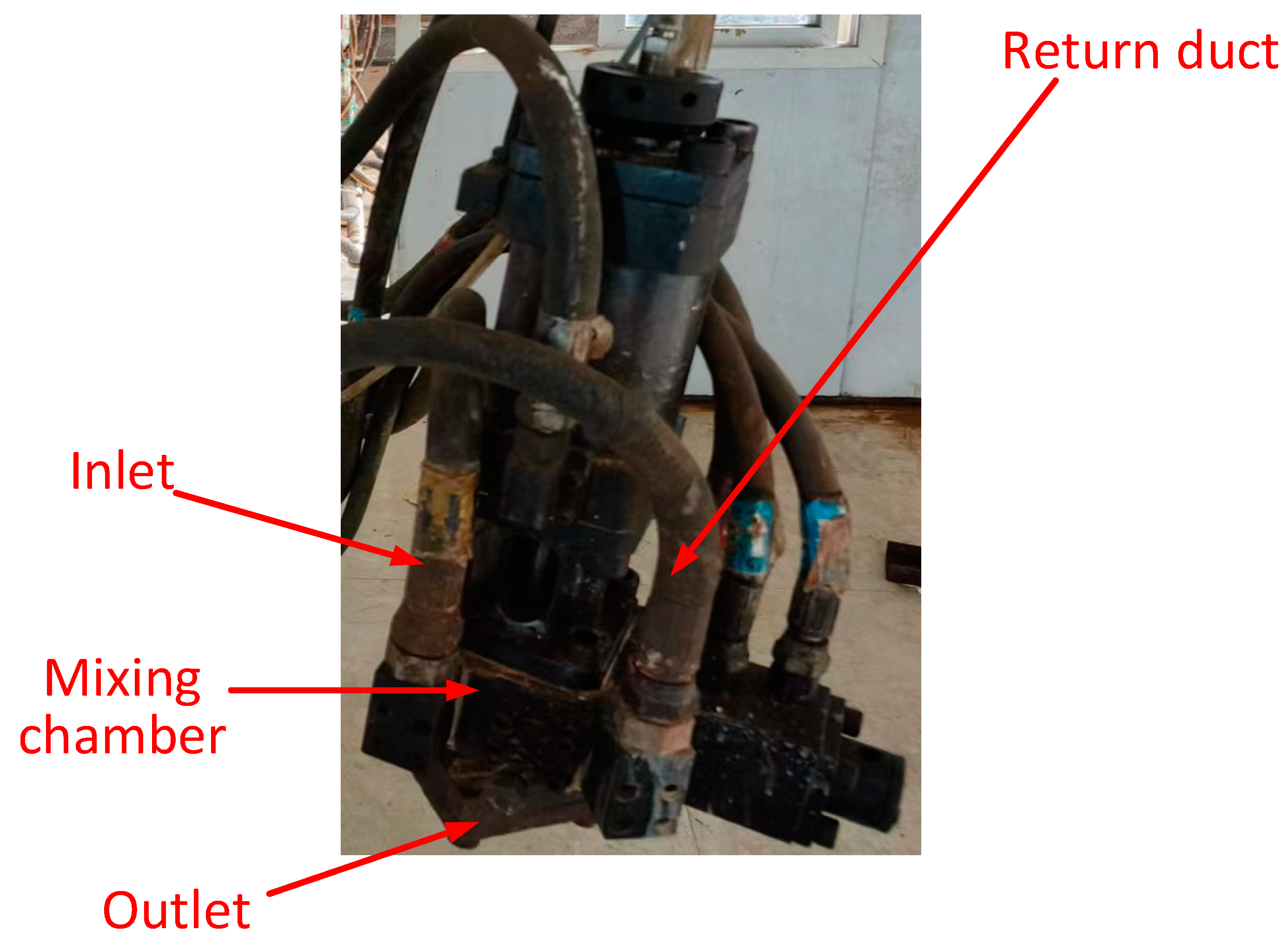
High-pressure mixers are essential for mixing polyimide materials, making the study of fluid flow characteristics within these mixers important. This research involves a simulated study of a high-pressure mixer (Figure 1) used in a polyimide foam production line. During operation, material flows into the mixer through the inlet and circulates back to the feed pipe via the return duct. When the pressure reaches the set value, the material enters the mixing chamber. Materials A and B mix and are ejected through the outlet into the mold.

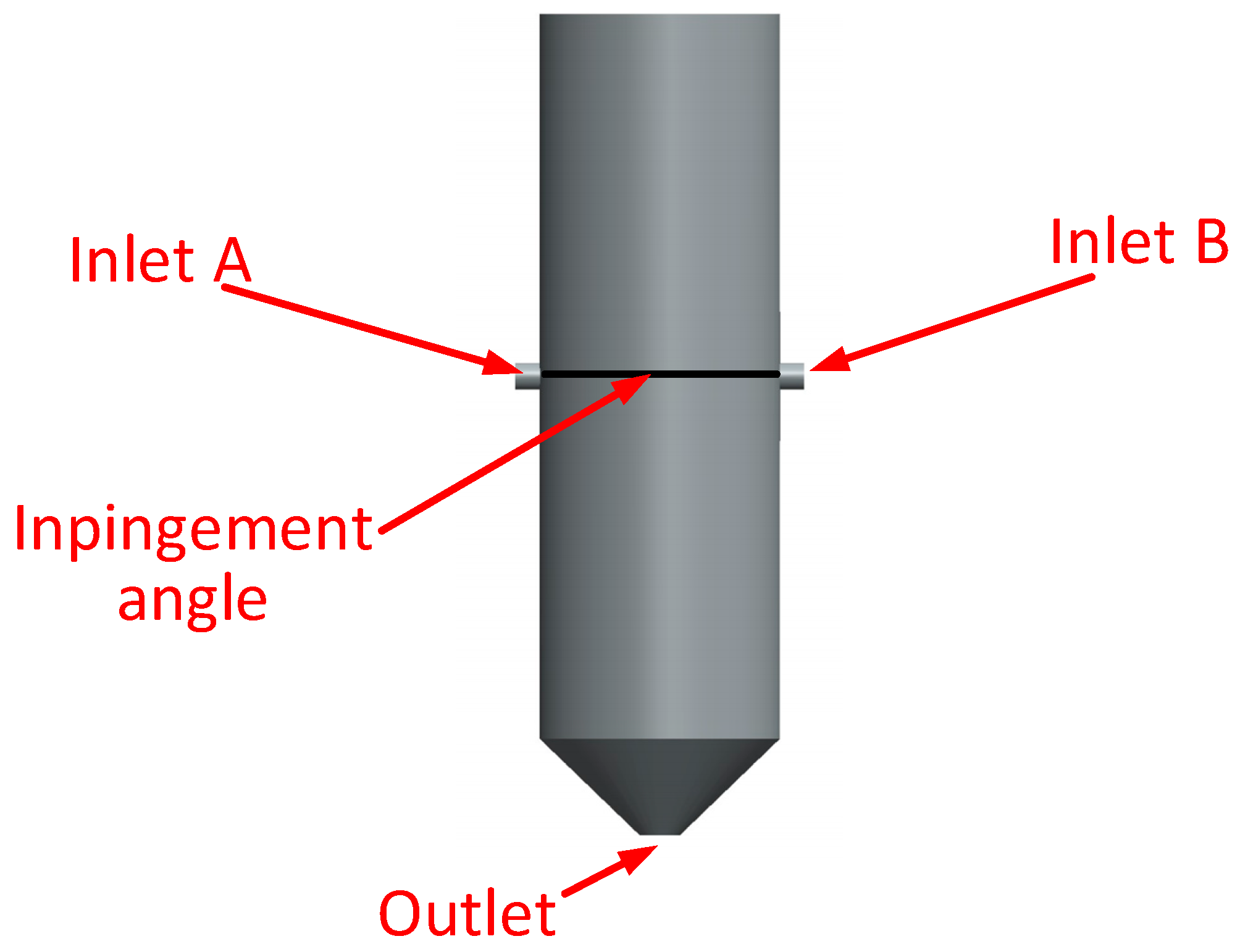
In the high-pressure mixer, materials A and B are fed into the mixing chamber through two separate inlets at a high speed and pressure by metering pumps, achieving high-speed collision mixing. The geometric model of the polyimide high-pressure mixer was created using 3D drawing software (Solidworks 2021) to explore the impact of the mixing head’s structural parameters and optimize its structure. The model was used for the fluid analysis of the high-speed collision mixing process of liquids A and B. The structure of the mixing chamber is shown in Figure 2. Materials A and B enter the chamber through inlets A and B. Inside, they collide and mix at high speed at a specific impingement angle determined by the two inlets. The shape of the fluid collision area is complex and irregular due to the high-speed, angled collision, generating intense turbulence and vortices. Rapid changes in the fluid velocity and direction after the collision result in highly irregular, nonlinear flow paths. Additionally, the significant velocity gradient within the collision area causes uneven material distribution and pronounced shear interactions between the fluids. These factors collectively contribute to the complexity and unpredictability of fluid flow within the mixing zone. After mixing, the materials exit the chamber through the outlet. The inlet diameters for components A and B are 8 mm, the outlet diameter is 35 mm, and the impingement angle is 180 degrees.

2.2. Mathematical Model

This section introduces the conservation laws of energy, mass, and momentum that fluid follows in a mixer. Based on the Navier–Stokes equation theory, a mathematical model is established. The mass and energy conservation equations are described, clarifying parameters like fluid density, velocity components, and temperature. The turbulence model, proposed by Launder and Spalding, is explained, detailing the relationship between turbulence energy, dissipation rate, and viscosity. The multiphase flow model is discussed, employing the Volume of Fluid (VOF) model to handle gas–liquid–liquid three-phase flow, introducing the continuity equations for each phase and the momentum conservation equation. These theories and equations provide a foundation for numerical simulations and analyses.

2.2.1. Reynolds Time-Averaged Control Equation

When fluid flows within a mixer, it adheres to the laws of conservation of energy, mass, and momentum. The mathematical model is established based on the theory of the Navier–Stokes control equations. The specific expression of these equations is as follows.

Mass conservation equation:

$${\displaystyle \frac{\partial \rho }{\partial t}}+{\displaystyle \frac{\partial (\rho \mu )}{\partial x}}+{\displaystyle \frac{\partial (\rho v)}{\partial y}}+{\displaystyle \frac{\partial (\rho w)}{\partial z}}=0$$

(1)

Vector form:

$${\displaystyle \frac{\partial \rho }{\partial t}}+\nabla \cdot (\rho v)=0$$

(2)

In the equation: $\mathsf{\rho }$—fluid density, with units in Kg/m³; u, v, w—velocity components in the x, y, z directions, respectively, in m/s.

Energy conservation equation:

$${\displaystyle \frac{\partial (\rho t)}{\partial t}}+div(\rho \overrightarrow{u}T)=div({\displaystyle \frac{k}{c_p}}gradT)+S_T$$

(3)

In the equation: C_p—specific heat capacity, with units in KJ/(kg×°C); T—temperature, in units K; k—fluid heat transfer coefficient; and S_T—viscous dissipation term.

$$\begin{array}{l}{\displaystyle \frac{\partial (\rho u)}{\partial t}}+{\displaystyle \frac{\partial (\rho uw)}{\partial x}}+{\displaystyle \frac{\partial (\rho vw)}{\partial y}}+{\displaystyle \frac{\partial (\rho ww)}{\partial z}}\\ =\rho f_z-{\displaystyle \frac{\partial p}{\partial z}}+{\displaystyle \frac{\partial (2\mu \frac{\partial u}{\partial z}+\overline{\lambda }div\mathrm{v})}{\partial z}}+{\displaystyle \frac{\partial [\mu (\frac{\partial v}{\partial z}+\frac{\partial u}{\partial x})]}{\partial x}}+{\displaystyle \frac{\partial [\mu (\frac{\partial w}{\partial y}+\frac{\partial u}{\partial z})]}{\partial y}}\end{array}$$

$$\begin{array}{l}{\displaystyle \frac{\partial (pu)}{\partial t}}+{\displaystyle \frac{\partial (puu)}{\partial x}}+{\displaystyle \frac{\partial (\rho vu)}{\partial y}}+{\displaystyle \frac{\partial (\rho wu)}{\partial z}}\\ =\rho f_x-{\displaystyle \frac{\partial p}{\partial x}}+{\displaystyle \frac{\partial (2\mu \frac{\partial u}{\partial x}+\overline{\lambda }div\mathrm{v})}{\partial x}}+{\displaystyle \frac{\partial [\mu (\frac{\partial v}{\partial x}+\frac{\partial u}{\partial y})]}{\partial y}}+{\displaystyle \frac{\partial [\mu (\frac{\partial w}{\partial x}+\frac{\partial u}{\partial z})]}{\partial z}}\end{array}$$

$$\begin{array}{l}{\displaystyle \frac{\partial (\rho v)}{\partial t}}+{\displaystyle \frac{\partial (\rho uv)}{\partial x}}+{\displaystyle \frac{\partial (\rho vv)}{\partial y}}+{\displaystyle \frac{\partial (\rho wv)}{\partial z}}\\ =\rho f_x-{\displaystyle \frac{\partial p}{\partial y}}+{\displaystyle \frac{\partial (2\mu \frac{\partial u}{\partial y}+\overline{\lambda }div\mathrm{v})}{\partial y}}+{\displaystyle \frac{\partial [\mu (\frac{\partial v}{\partial x}+\frac{\partial u}{\partial y})]}{\partial x}}+{\displaystyle \frac{\partial [\mu (\frac{\partial w}{\partial x}+\frac{\partial u}{\partial z})]}{\partial z}}\end{array}$$

(4)

In Equation (4), u, v, w—velocity components in the x, y, z directions, respectively, in m/s; ρ—fluid density, in kg/m³; P—static pressure, in Pa; and μ—molecular viscosity, in Pa·s.

2.2.2. Turbulence Model

The standard model, proposed by Launder and Spalding, is a predominant tool in engineering flow field computations due to its broad applicability, cost-effectiveness, and accuracy. It is recognized as the simplest model producing effective computational outcomes, especially in simulating a single-phase fluid flow within stirred tanks. Consequently, this turbulence model is chosen to address turbulence in mixers. In this model, the relationship among turbulence energy k, the rate of turbulence dissipation $\mathit{\epsilon }$, and the turbulent viscosity ${\mathsf{\mu }}_{\mathrm{t}}$ is represented as follows:

$${\mu }_t=\rho C_{\mu }{\displaystyle \frac{k^2}{\epsilon }}$$

(5)

The turbulence kinetic energy k equation is:

$${\displaystyle \frac{\partial (\rho k)}{\partial t}}+{\displaystyle \frac{\partial (\rho k{\mu }_i)}{\partial x_i}}={\displaystyle \frac{\partial [(\mu +\frac{{\mu }_t}{{\sigma }_k})\frac{\partial k}{\partial x_j}]}{\partial x_j}}+G_k-\rho \epsilon$$

(6)

The equation for the turbulence energy dissipation rate is:

$${\displaystyle \frac{\partial (\rho \epsilon )}{\partial t}}+{\displaystyle \frac{\partial (\rho \epsilon u_i)}{\partial x_i}}={\displaystyle \frac{\partial [(\mu +\frac{\mu }{{\sigma }_{\epsilon }})\frac{\partial \epsilon }{\partial x_j}]}{\partial x_j}}+{\displaystyle \frac{C_{1\epsilon }}{k}}{G}_k-C_{2\epsilon }\rho {\displaystyle \frac{{\epsilon }^2}{k}}$$

(7)

The production term of the turbulent kinetic energy k due to the mean velocity is calculated by the following expression:

$$G_k=\mu ({\displaystyle \frac{\partial u_i}{\partial x_j}}+{\displaystyle \frac{\partial u_j}{\partial x_i}}){\displaystyle \frac{\partial u_i}{\partial x_j}}$$

(8)

2.2.3. Multiphase Flow Model

Extensive numerical simulations have demonstrated [24,25,26,27,28] that the VOF model exhibits an excellent performance in managing both steady-state and transient gas–liquid interfaces. This study examines a gas–liquid–liquid three-phase flow, employing the VOF multiphase flow model. The continuity equations for each phase are as follows:

$${\rho }_q{\displaystyle \frac{\partial {\alpha }_q}{\partial t}}+\nabla (U\overrightarrow{{\alpha }_q}{\rho }_q)=S_{{\alpha }_q}+{\displaystyle \sum _{p=1}^n(\stackrel{•}{m_{pq}}-\stackrel{•}{m_{pq}})}$$

(9)

In these equation, p and q denote different phases; ${\mathsf{\rho }}_{\mathrm{q}}$ is the density of phase q; t represents time; $\mathsf{\alpha }$ is the volume fraction; U is the velocity at any point in the flow field; ${\mathrm{S}}_{{\mathsf{\alpha }}_{\mathrm{q}}}$ indicates the source phase; and ${\stackrel{•}{\mathrm{m}}}_{\mathrm{pq}}$ and ${\stackrel{•}{\mathrm{m}}}_{\mathrm{qp}}$ are the mass transfer rates between the two phases.

In the VOF model, all phases share a single velocity field. The momentum conservation equation is given by:

$${\displaystyle \frac{\partial }{\partial t}}(\rho \overrightarrow{U})+\nabla •(\rho \overrightarrow{U}\overrightarrow{U})=-\nabla P+\nabla •[\mu (\nabla \overrightarrow{U+U^T)}]+\rho g+\overrightarrow{F}$$

(10)

2.3. Numerical Solving Method

The standard k-ε model is used to solve the flow within the mixer. The inlets for materials A and B both use pressure inlet boundary conditions, with the pressure at the inlets set to the impingement pressure. The inner walls of the mixer are treated as stationary walls. Gravity is also considered, with its direction being perpendicular to the outlet plane. The pressure–velocity coupling method utilizes the SIMPLE algorithm, with pressure discretization using PRESTO! All other discretization schemes adopt a second-order upwind scheme, with under-relaxation factors set to default values and variable residuals all set to 10⁻⁶. Additionally, the VOF multiphase flow model is incorporated. According to actual working conditions, fluids A and B are selected as working substances. Fluid A has a density of 1.17 g/cm³ and a viscosity of 0.16 Pa·s; fluid B has a density of 1.25 g/cm³ and a viscosity of 0.36 Pa·s, with an operating pressure of 10 MPa. Because the fluid’s mixing time within the mixer is brief, and the viscosity has a minimal impact on the mixing performance. To simplify the calculations, the following assumptions are made: (1) no reactions occur within the mixer; (2) temperature and pressure effects on viscosity are neglected; and (3) the flow field within the mixer is considered as a three-dimensional, steady, isothermal, incompressible viscous fluid in stable turbulent flow.

2.4. Grid Partitioning and Investigation of Grid Independence

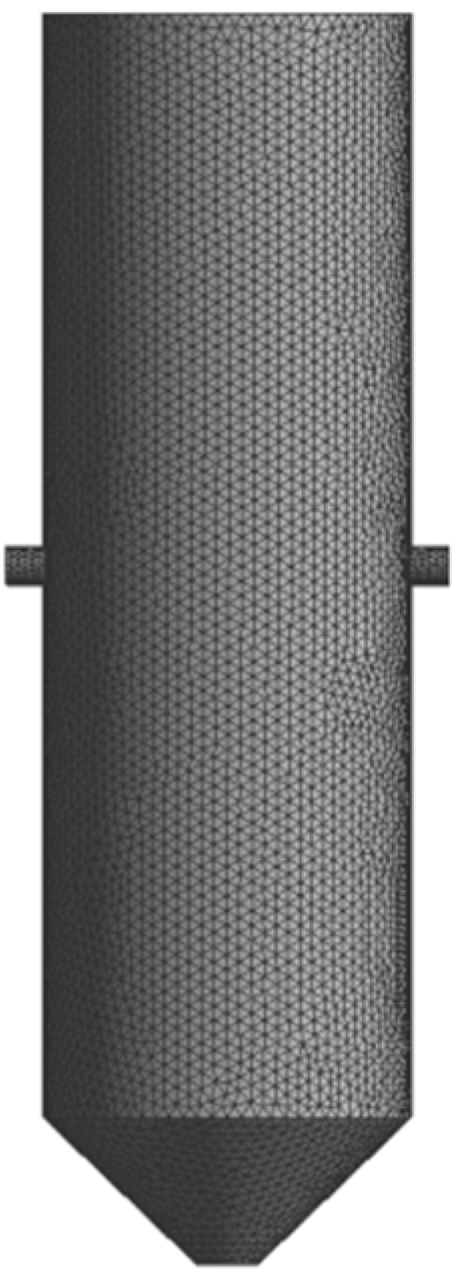
The mixer was meshed using the grid function in Fluent software (Fluent 2022). As the study focuses on impingement mixing effects rather than flow details near the wall, the boundary layer was not considered. This simplifies the model and conserves computational resources. Due to the complexity and irregular shape of the fluid collision area, the number of grids significantly affects calculation accuracy. Too many grids increase the computational burden and prolong calculation time, while too few compromises precision. Therefore, selecting an appropriate number of grids is essential. The mesh element quantities for the five sets of plans are listed in

Table 1. Mesh element quantities for five plans.

Plan	Number of Mesh Elements
Plan 1	58,574
Plan 2	63,874
Plan 3	86,824
Plan 4	146,142
Plan 5	221,348

, and the resulting pressure drop is shown in Figure 3.

From Figure 3, it is observed that when the number of grids reaches 146,142, the pressure drop remains nearly constant. Therefore, the selected number of grids for calculation is 146,142. The results of the mesh division are shown in Figure 4. The quality of the mesh elements is greater than 0.444, meeting the computational and accuracy requirements.

2.5. Results Analysis and Discussion

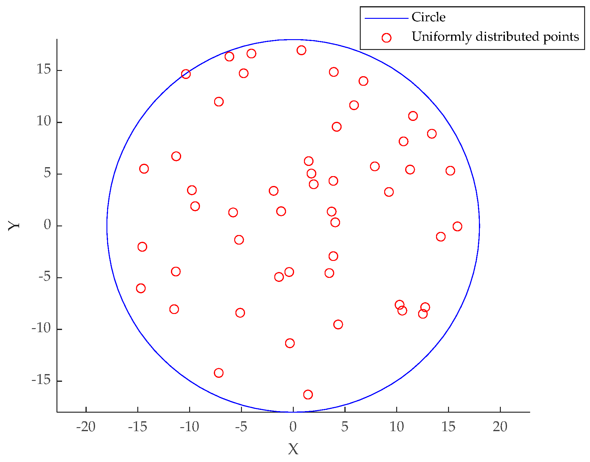
This section evaluates the mixing performance of the mixer through both qualitative and quantitative analyses methods. The qualitative method includes plotting density contour maps of the outlet cross-section and observing color bands and distributions to assess mixing uniformity. The quantitative method uses the root mean square deviation of the liquid density at various sampling points to measure mixing quality. The specific steps involve, after completing numerical calculations, uniformly selecting liquid density values from nodes on the outlet cross-section for calculation.

2.5.1. Mixer Mixing Performance Evaluation Index

To ensure the accuracy of the conclusions, both qualitative and quantitative analyses are employed to evaluate the mixing effects. The qualitative method involves plotting a density contour map of the outlet section to observe color bands and distribution, determining the uniformity of the mixing.

The quantitative method uses mixing unevenness, the root mean square deviation of the liquid density at various points. This metric represents the degree of difference between the liquid density at the sampling points and the average liquid density of the mixing system under investigation. Thus, this article uses the root mean square deviation of the density values on the mixer’s outlet cross-section to assess the mixing quality of the designed mixer. The S parameter can be determined:

$$S=\sqrt{{\displaystyle \frac{{\displaystyle \sum _{i=1}^n{({\rho }_i-\overline{\rho })}^2}}{(n-1)}}}/\overline{\rho }$$

(11)

In Equation (11), $\mathsf{\rho }$ represents the liquid density, and n stands for the number of sample points. Generally, the smaller the mixing unevenness, the smaller the difference in liquid density across the cross-section, indicating a smaller density gradient and better mixing quality.

To compute the mixing index, after the numerical calculations are completed, the liquid density values at 50 uniformly selected nodes on the outlet cross-section are taken, as shown in Figure 5.

2.5.2. Simulation Results

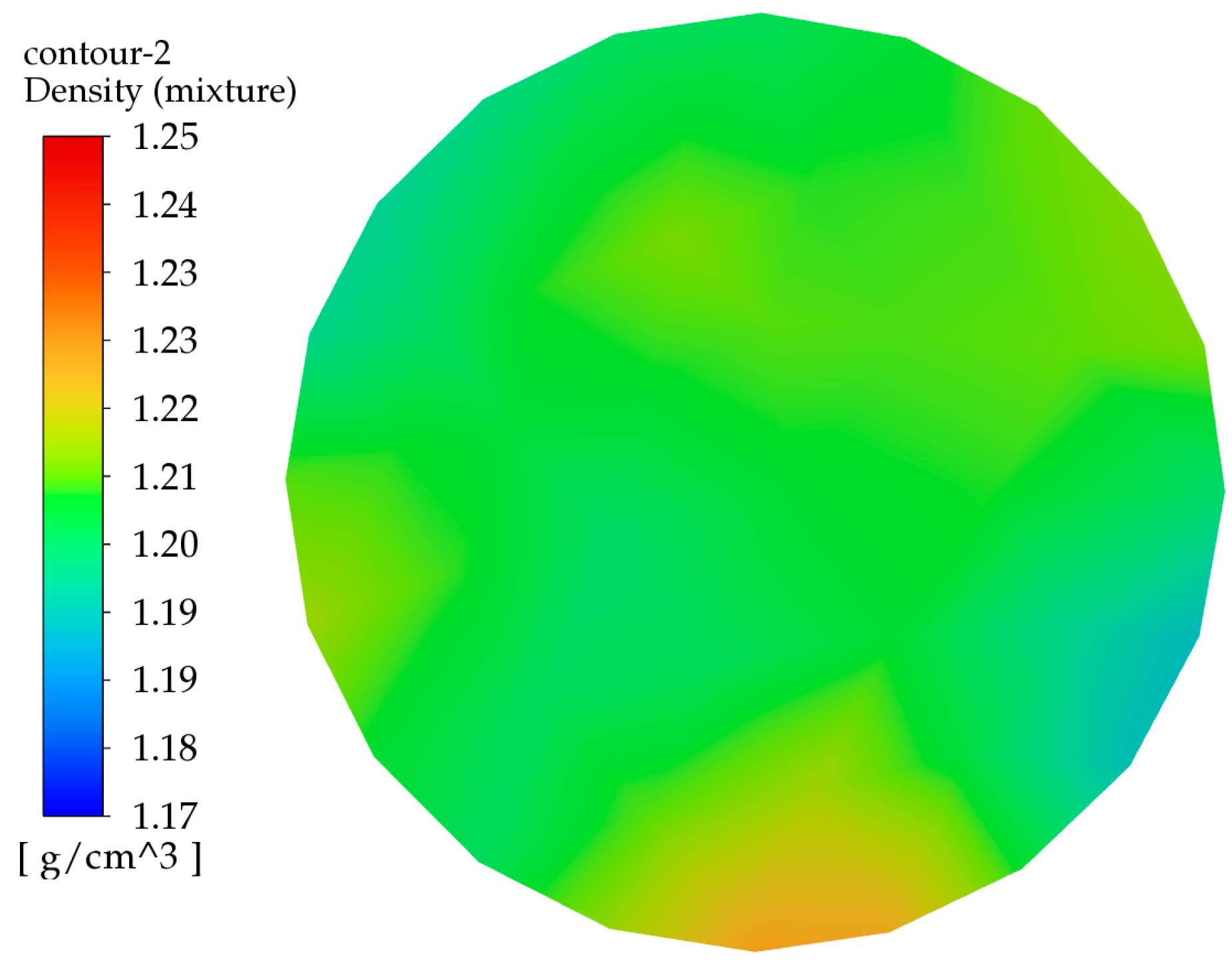
To improve the mixing performance of the mixer head, an internal flow field analysis is conducted. Based on the prototype mixer, the effect of the mixer head’s geometric parameters on mixing efficiency is investigated by altering dimensions such as the inlet diameter, outlet diameter, impingement angle, and impingement pressure. This serves as a foundation for further explorations into enhancing mixing efficiency and optimizing the mixer’s structure. After setting the boundary conditions, the flow field analysis of the mixing head is conducted. A density contour plot for the outlet section of the mixing head is generated to make the results more visually intuitive. The figures used in this document are exclusively density contour plots. The relevant density contour plot is shown in Figure 6.

As shown in Figure 6, the density is greater toward the middle sides and the lower middle side, with less density on the left side and the lower right side. Given the 1:1 mixing ratio of the materials, thorough mixing would result in fewer color bands, and the density should be between 1.20 and 1.21 g/cm³. In the figure, the high-density and low-density areas occupy a larger proportion, indicating that the surface mixing effect is poor and further optimization is needed.

The calculated mixing unevenness of the original mixing head is 0.11, indicating a poor mixing performance. The structure of the original mixing head is optimized to improve the mixing effect.

3. Full Factorial DOE and Significance Analysis of Influencing Factors

In this chapter, a full factorial DOE was used to analyze the significance of four parameters affecting the mixer’s performance. A factor level table was established, and the mixing unevenness for each experimental group was calculated. Finally, factor analysis was conducted to determine the impact of each parameter on the mixer’s performance, laying the foundation for subsequent structural optimization.

3.1. Full Factorial DOE

Experimental design is a common statistical method, including confounding, response surface, full factorial, and fractional factorial designs. The full factorial DOE is a classic method characterized by its comprehensive nature, typically including two or more factors, each with multiple levels. This approach encompasses all combinations, providing a complete understanding of factor interactions. When designing a full factorial DOE, researchers consider which factors could impact results and select variables accordingly. The use of full factorial DOE helps researchers understand various factors in an experiment, but key factors, like sample size and repeatability, must also be considered to ensure accuracy and reliability.

Taking mixing unevenness as the experimental impact index, four factors—mixer inlet diameter D₁, outlet diameter D₂, impinging angle θ, and impinging pressure P—were chosen as screening parameters. Each factor was set at two levels according to the experimental design requirements. The two-level values for these four parameters are detailed in

Table 2. Factor-level table.

Parameters [Unit]	Value1	Value
D1 [mm]	8	16
D2 [mm]	25	45
θ [°]	60	180
P [MPa]	8	20

. The mixer inlet diameter D₁ ranges from 8 mm to 16 mm, the outlet diameter D₂ is set at 25 mm and 45 mm, the impinging pressure P is set at 8 MPa and 20 MPa, and the impinging angle θ is set at 60° and 180°.

A two-level full factorial DOE was conducted on the four parameters, yielding 19 sample points. For the experimental design of the mixer’s structural parameters, this meant obtaining 19 slightly different mixer models. Simulation analyses were separately performed on these mixer models, yielding the mixing unevenness (S) for each model, as shown in

Table 3. Full factorial DOE results.

S.N	D1 [mm]	D2 [mm]	P [MPa]	θ [°]	S
1	16	25	20	180	0.600989
2	16	45	20	60	0.653101
3	16	45	8	180	0.742879
4	6	25	8	180	0.824658
5	6	25	8	60	0.795684
6	11	35	14	120	0.239548
7	16	25	8	60	0.593242
8	16	45	8	60	0.644044
9	11	35	14	120	0.238963
10	11	35	14	120	0.233965
11	6	45	8	180	0.832547
12	6	45	20	60	0.429569
13	6	45	20	180	0.826549
14	6	45	8	60	0.448426
15	16	25	8	180	0.614530
16	6	25	20	180	0.815843
17	6	25	20	60	0.786324
18	16	45	20	180	0.717372
19	16	25	20	60	0.551930

.

3.2. Factor Analysis

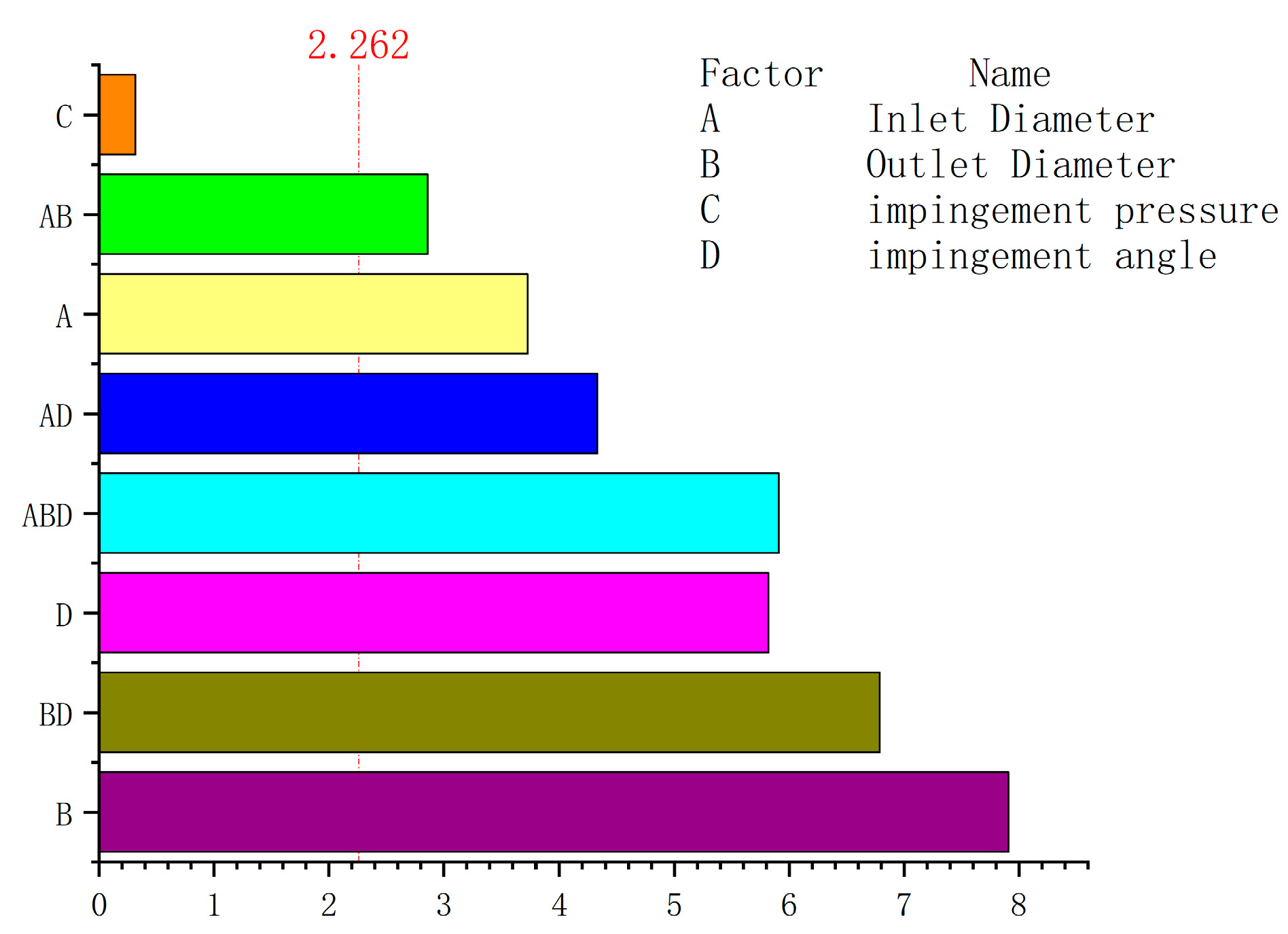
To analyze the impact of varying structural parameters on mixing unevenness, factor analysis was conducted using the simulation results of the mixing head flow field. The numerical simulation results were used as the ordinate, and the levels of its four structural parameters were used as the abscissa. The experimental data were processed with MINITAB, resulting in a pareto chart of the standardized effects of the response variables, as shown in Figure 7. From Figure 7, it is evident that the inlet diameter, outlet diameter, and impingement angle significantly impact the mixing effect, while the effect of impingement pressure is relatively small. The influence order of each structural parameter on mixing unevenness is: mixer outlet diameter > impingement angle > inlet diameter > impingement pressure. It can be observed from the figure that the impact of impingement pressure on the mixing effect is minimal and can therefore be disregarded.

4. Optimization of Mixing Head Structure

In this chapter, the mixer’s structure is optimized using a joint optimization algorithm combining SSA-CNN-LSTM and the WOA. Initially, the optimization objectives were determined, and a sample library was established using OLH. Subsequently, an SSA-CNN-LSTM prediction model was constructed and compared with CNN-LSTM and LSTM prediction models. Finally, the WOA was employed to optimize the constructed prediction model to obtain the optimal structural parameters.

4.1. SSA-CNN-LSTM-WOA Optimization Process

This paper optimizes the structural parameters of the polyimide mixer to minimize mixing unevenness. Four structural parameters were selected for significance analysis to determine their impact and eliminate insignificant ones, thereby reducing computational effort. The proposed optimization process combines sample extraction, approximate model establishment, and optimization algorithms. OLH was used to select samples for training the approximate model, and numerical simulation results for each sample were computed. An SSA-CNN-LSTM surrogate model was constructed to fit the relationship between optimization objectives and variables. The WOA was used to find the optimal solution. If the optimization results meet the design requirements, the search is concluded, and the results are subjected to simulation and experimental validation. If the results are unsatisfactory, variables are reselected for further optimization until the requirements are met. Figure 8 illustrates the mixer optimization process based on the SSA-CNN-LSTM-WOA.

4.2. Selection of Optimization Objectives

From the full factorial DOE, it is evident that impingement pressure has a minimal impact on mixing uniformity. Hence, the inlet diameter, outlet diameter, and impingement angle are chosen as the optimization variables. Thus, establishing its mathematical model for optimization. The optimization model consists of three factors: the design objective, variables, and constraints. The minimum mixing unevenness of the mixing head is the optimization goal. The impingement angle, inlet diameter, and outlet diameter are the design variables. The constraints are the value ranges of these variables. The mathematical model is shown in Equation (12).

$$\left\{\begin{array}{l}W=F(S)\to \min \\ S=f(D_1,D_2,\theta )\\ 6\le D_1\le 16\\ 25\le D_2\le 45\\ 60\le \theta \le 180\end{array}\right.$$

(12)

In Equation (12):

• W—represents the optimization objective function of the mixer;
• D₁—denotes the inlet diameter of the mixer;
• D₂—denotes the outlet diameter of the mixer;
• θ—represents the impingement angle.

4.3. Construction and Validation of the SSA-CNN-LSTM Model

This section employs OLH to extract a certain number of samples, followed by the construction of an SSA-CNN-LSTM prediction model. The model is evaluated using Mean Absolute Error (MAE), Mean Absolute Percentage Error (MAPE), and Root Mean Square Error (RMSE) as performance metrics. To demonstrate the superiority of the SSA-CNN-LSTM model, comparative analyses are conducted with CNN-LSTM and LSTM models.

4.3.1. Establishment of Training Samples

Before constructing the model, multiple sets of samples must be obtained to serve as training data, ensuring they are uniformly distributed within the design space. This paper selects three optimization variables. Manually assigning samples often leads to an uneven distribution, resulting in training data that do not adequately represent the sample space. Therefore, uniform sampling and Latin Hypercube Sampling (LHS) are commonly used.

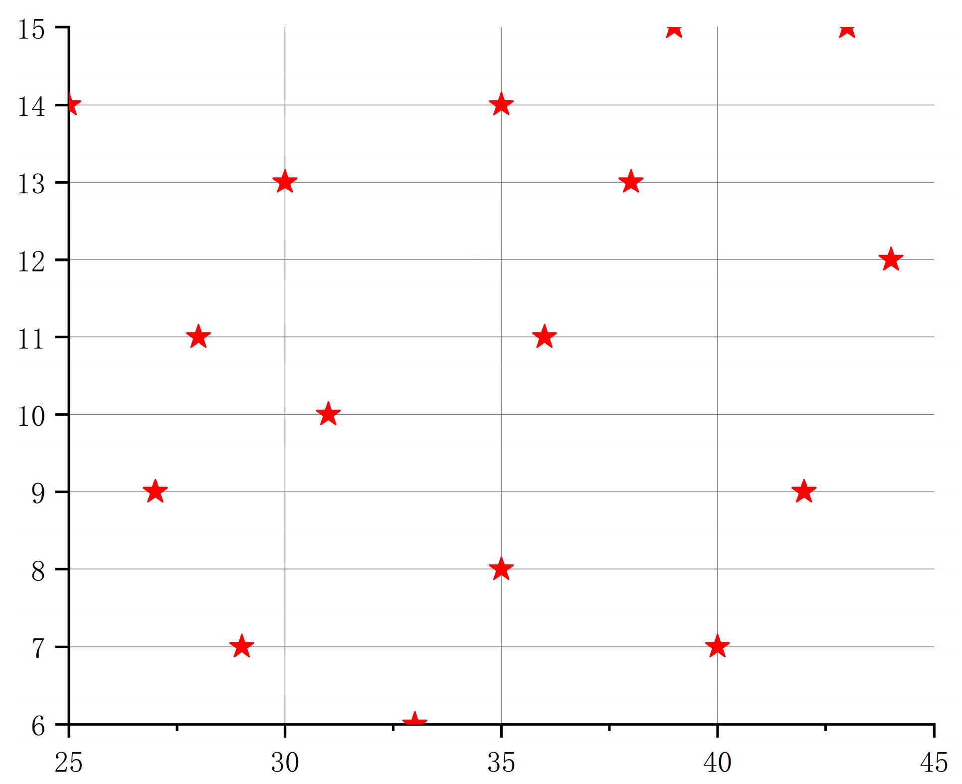
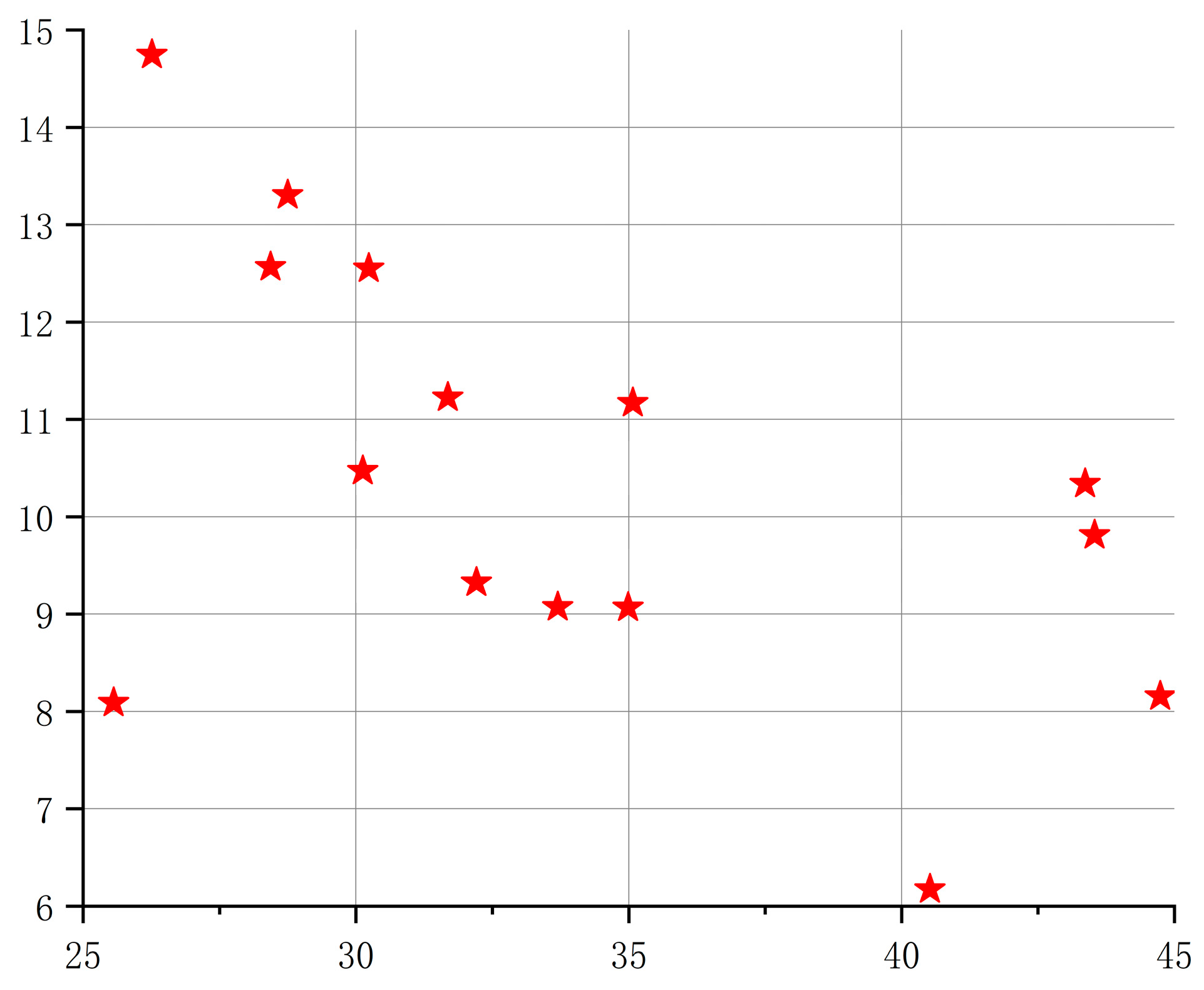
Uniform sampling considers only the distribution of samples, without ensuring they are neat and comparable. Scholars later proposed the LHS method, which divides the sample space into equidistant single spaces and randomly takes one sample from each. This method is efficient and stable, but the samples are not uniformly distributed within the design space. To better represent the sampling space, OLH was developed as an improvement to LHS. OLH is a stochastic multidimensional stratified sampling approach that divides the probability distribution function of experimental factors into N non-overlapping sub-regions based on the value ranges of the influencing factors, with independent equal-probability sampling within each sub-region. Compared to orthogonal experiments, LHS offers more flexible grading of level values, and the number of experiments can be manually controlled. However, the experimental points may still not be evenly distributed, and as the number of levels increases, some regions of the design space may be missed. OLH improves upon LHS, enabling uniform, random, and orthogonal sampling within the design space of experimental factors, allowing substantial model information to be acquired with relatively few sampling points [29]. Figure 9 shows the results of 16 samples at 2 levels of OLH, demonstrating that this method better fills the sampling space. Figure 10 shows the sampling results of LHS.

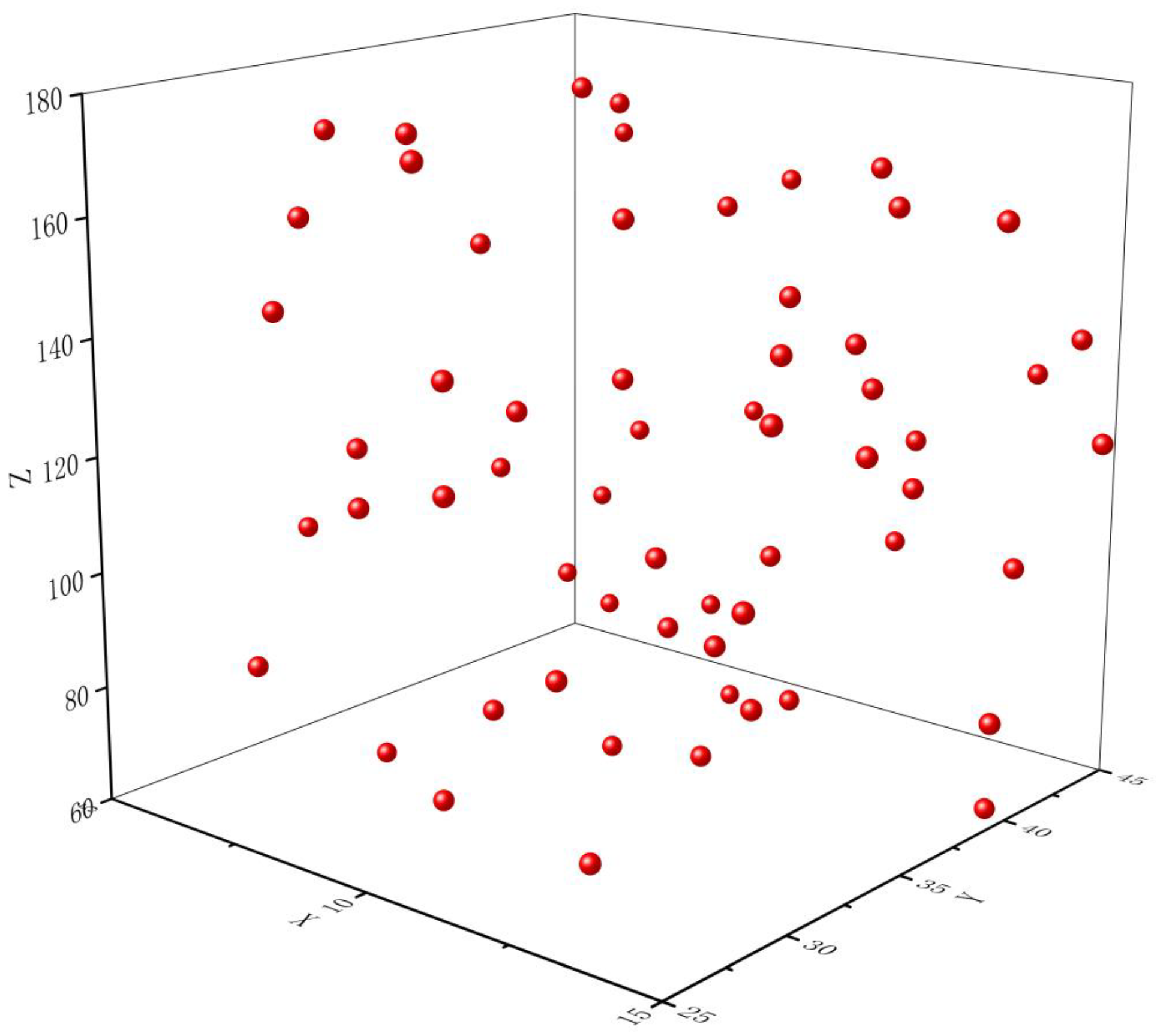
The training samples should be at least ten times the number of input variables. To ensure credible results, this paper uses OLH to draw 60 sample points from the sample space, as depicted in Figure 11. Based on these samples, 60 mixer models are constructed in 3D drawing software, resulting in 60 CFD computational models. The numerical simulation method is identical to the one used for the prototype mixer discussed earlier, producing 60 sets of data for mixing unevenness corresponding to 60 sets of parameters. A sample database is established, as shown in

Table 4. Sample library.

S.N	D2 [mm]	D1 [mm]	θ [°]	S	S.N	D2 [mm]	D1 [mm]	θ [°]	S
1	27	9	85	0.565601332	31	40	16	161	0.792021249
2	36	8	66	0.695298038	32	40	6	70	0.658225944
3	29	11	76	0.439453453	33	30	16	167	0.277265494
4	44	7	71	0.604243547	34	28	13	93	0.32291663
5	35	9	160	0.039434946	35	34	10	129	0.388527015
6	36	15	122	0.230791242	36	31	12	132	0.288808952
7	35	8	123	0.090646802	37	29	14	107	0.48610121
8	28	10	150	0.03733436	38	42	13	110	0.420938856
9	40	7	142	0.156511798	39	37	8	170	0.220676555
10	38	10	66	0.433840623	40	27	14	80	0.379446807
11	44	9	101	0.358081664	41	38	6	154	0.246376589
12	32	9	72	0.53680958	42	39	12	117	0.539765996
13	32	10	89	0.33418985	43	37	6	61	0.615474219
14	26	8	176	0.730686246	44	35	16	165	0.508707806
15	28	13	110	0.566211296	45	30	11	131	0.314845462
16	31	14	96	0.571509591	46	31	9	139	0.409969816
17	34	9	178	0.102667462	47	41	12	157	0.159976293
18	26	14	144	0.513248826	48	43	12	88	0.470201261
19	27	7	115	0.036445866	49	34	14	155	0.171068748
20	32	12	175	0.76855878	50	25	13	127	0.080966932
21	39	15	169	0.687295763	51	37	15	105	0.661896866
22	34	13	164	0.464086254	52	44	11	138	0.665976529
23	41	11	140	0.743605475	53	29	11	148	0.503747507
24	33	10	74	0.547576058	54	28	7	80	0.446037397
25	39	13	82	0.359809661	55	37	14	119	0.16558753
26	44	12	135	0.405659276	56	45	7	114	0.546648081
27	42	15	126	0.607806714	57	25	15	90	0.570496729
28	42	8	104	0.135733924	58	38	8	99	0.252273179
29	33	7	151	0.220021216	59	43	10	173	0.814712302
30	42	15	63	0.46109265	60	32	11	95	0.209671239

.

4.3.2. Construction of the SSA-CNN-LSTM Model

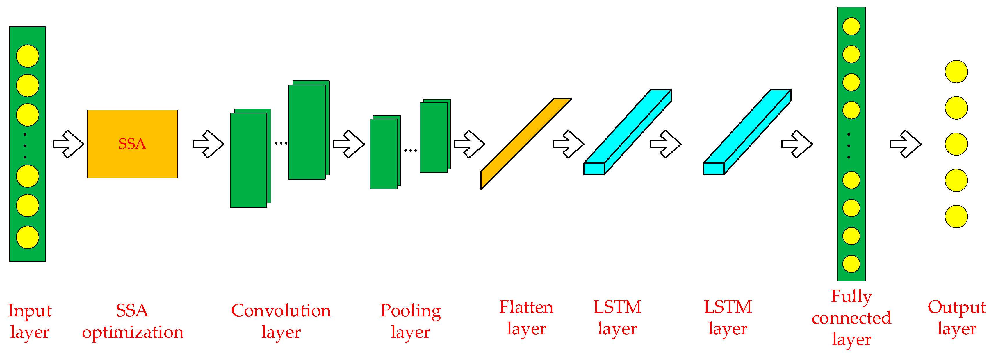
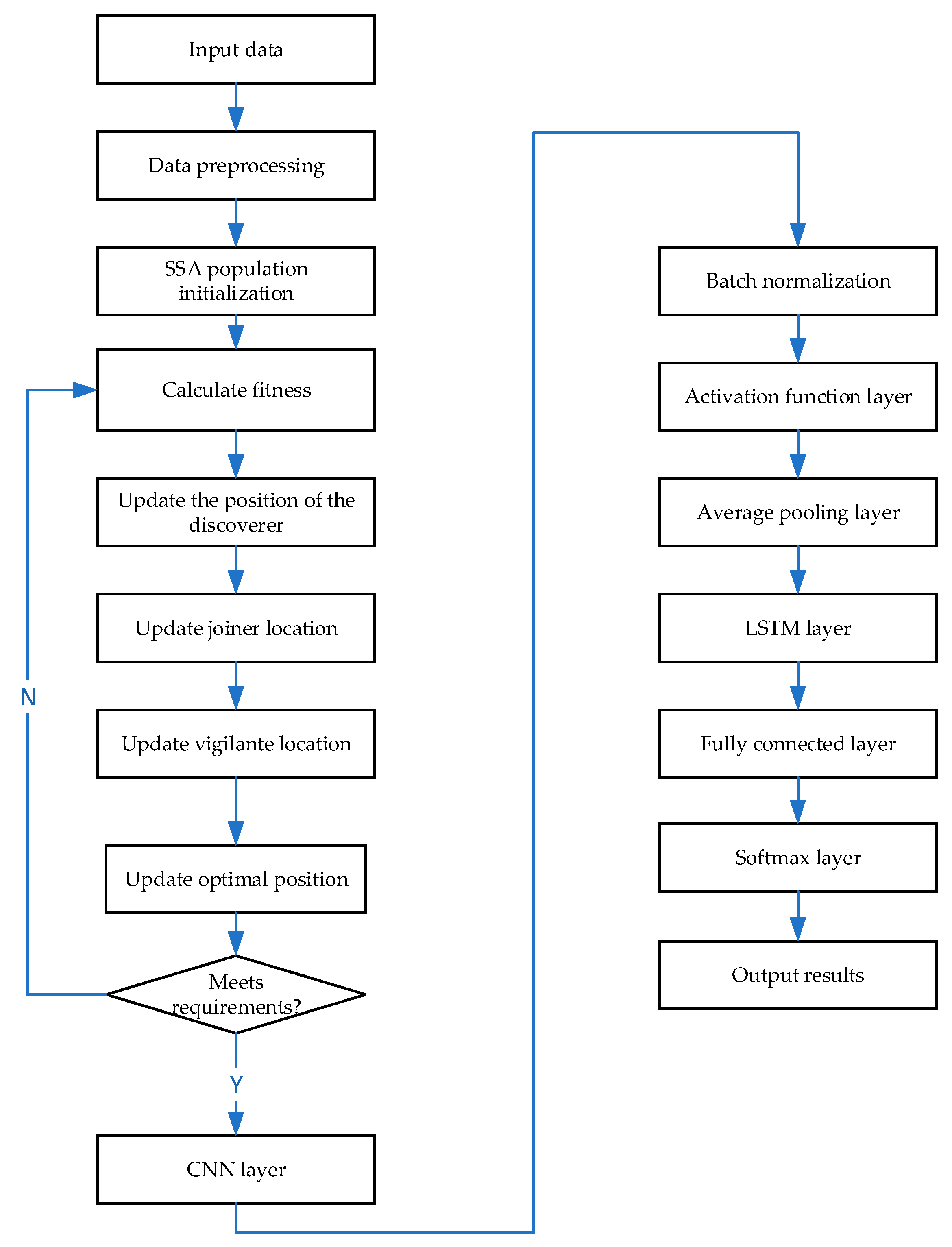
In the CNN-LSTM model, SSA adjusts various parameters to enhance performance. The network structure has three main components: CNN for extracting spatial features, LSTM for learning time series information, and SSA for optimizing parameters (e.g., number of convolutional kernels and LSTM units). Input data pass through the CNN to extract spatial features, then into the LSTM to learn time-series information. SSA optimizes parameters through iterative searching and updating. Ultimately, this optimized model can be used for data prediction tasks.

The application of the SSA to optimize the CNN-LSTM model involves the following steps:

(1)

Data preprocessing: data labeling, dataset division, data normalization, and data format conversion;

(2)

SSA population initialization: setting the initial size of the sparrow population (n), the maximum number of iterations (N), the proportion of discoverers (PD), the number of sparrows perceiving danger (SD), the safety value (ST), and the alert value (R2);

(3)

Computing fitness, updating discoverer positions, updating joiner positions, updating scrounger positions, and updating the optimal individual position;

(4)

Feeding data into the CNN network, passing data through CNN layers, batch normalization layers, activation function layers, and average pooling layers;

(5)

Entering data into the LSTM neural network after going through LSTM layers to the fully connected layer and SoftMax layer;

(6)

Outputting the results.

Although the SSA algorithm has global search capabilities and adaptability, it is sensitive to the selection of initial parameters and requires tuning for specific problems. When optimizing the CNN-LSTM model, carefully selecting appropriate optimization objectives and fitness functions ensures the SSA algorithm significantly enhances performance. The parameters optimized by SSA mainly include the number of neurons in the LSTM layer, convolution kernel size, number of convolutional layers, number of neurons in the fully connected layer, and learning rate. The schematic diagram of the SSA-CNN-LSTM model is shown in Figure 12.

(1)

Number of neurons in the LSTM layer: The LSTM layer is an important part of the CNN-LSTM model, and the choice of the number of neurons directly affects the performance of the model. Through the SSA algorithm, the optimal number of neurons in the LSTM layer can be dynamically searched, thereby improving the model’s prediction accuracy.

(2)

Convolution kernel size: The convolution operation in the CNN-LSTM model is very important for extracting spatial features of the data, and the choice of convolution kernel size will affect feature extraction. The SSA can optimize the size of the convolution kernel to further improve the accuracy of the model.

(3)

Number of convolutional layers: The deeper the convolutional layers in the CNN-LSTM model, the greater the computational cost required during forward propagation, but the accuracy of the model will also increase correspondingly. By optimizing the number of convolutional layers, the SSA algorithm can enhance model accuracy within an acceptable range of computational costs.

(4)

Number of neurons in the fully connected layer: The number of neurons in the fully connected layer determines the output dimension and prediction ability of the model. By optimizing the number of neurons in the fully connected layer, the SSA can improve the accuracy and generalization ability of the model.

(5)

Learning rate: The CNN-LSTM model needs to specify a learning rate during training. Too high or too low a learning rate will affect the convergence and accuracy of the model. The SSA can search for the optimal learning rate to improve the efficiency and accuracy of model training. Combining the above module construction steps, the flowchart of the SSA-CNN-LSTM model is shown in Figure 13.

4.3.3. Benchmark Methods and Evaluation Criteria

In the comparative study of models, this paper adopts the following two machine learning models:

(1)

LSTM Model

LSTM is a type of Recurrent Neural Network (RNN) with two gates and one cell state, allowing it to store data longer than standard RNNs. The gates regulate information flow by specifying activation functions within the LSTM cell. The LSTM model in this paper consists of four consecutive pairs of LSTM and Dropout layers. The Dropout layers reduce dependency on previous data, and the final output is obtained through a fully connected layer.

(2)

CNN-LSTM Model

The CNN-LSTM model can achieve multi-feature classification prediction. The CNN is used for feature (fusion) extraction, and then the extracted features are mapped as sequence vectors input into the LSTM.

To evaluate the effectiveness and applicability of the prediction models on the dataset, three common evaluation metrics are used to quantify the precision and errors of predictions, namely MAE, MAPE, and RMSE.

The calculation for MAE is shown below; it represents the average of the absolute errors and can reflect the actual situation of prediction errors.

$$MAE={\displaystyle \frac{1}{z}}{\displaystyle \sum _{i=1}^z\left|y_i-{\widehat{y}}_i\right|}$$

(13)

The calculation for MAPE is as follows, representing the fitting effect and precision of the prediction model.

$$MAPE={\displaystyle \frac{1}{z}}{\displaystyle \sum _{i=1}^z\frac{\left|y_i-{\widehat{y}}_i\right|}{y_i}}$$

(14)

RMSE measures the deviation between the actual and the predicted values, with its calculation shown as below.

$$RMSE=\sqrt{{\displaystyle \frac{1}{z}}{\displaystyle {\sum }_{i=1}^z{(y_i-{\widehat{y}}_i)}^2}}$$

(15)

where z represents the number of samples, ${\mathrm{y}}_{\mathrm{i}}$ is the actual value, and ${\hat{\mathrm{y}}}_{\mathrm{i}}$ is the predicted value. These three indicators represent different aspects of the predictive performance, and the smaller their values, the better the performance.

4.3.4. Experimental Parameter Settings

In this section, the SSA-CNN-LSTM model is employed for predicting mixing unevenness. The model optimizes CNN-LSTM using the SSA, with parameters including the number of iterations (M), population size pop, the proportion of discoverers (p_percent), fitness function (f_n), and the dimension of parameters to be optimized (dim).

(1)

Number of iterations (M): This parameter determines the computation time and accuracy of the algorithm. Typically, the more iterations, the longer the computation time and the higher the accuracy. Here, it is set to 50.

(2)

Population size (pop): This refers to the number of sparrows used for computation, with no explicit rule for its size. Typically, it is based on a specific analysis of the problem at hand. For optimizing general problems, setting 50 sparrows is sufficient to solve most issues. For particularly difficult or specified problems, it might be necessary to increase the population size. Generally, the smaller the population size, the easier it is to fall into local optima, while a larger population size results in slower convergence. Here, the population size is set to 50.

(3)

Proportion of discoverers (p_percent): The percentage of discoverers in the population, set here to 20%.

(4)

The percentage of sparrows that are aware of danger is set to 10%.

(5)

Safety threshold (ST) is set to 0.8.

(6)

Fitness function (f_n): Determines the fitness of a sparrow’s position.

(7)

Parameter dimension (dim): Indicates the number of parameters to be optimized. Here, optimization is applied to three parameters of the LSTM layer, which are the optimal number of neurons, the optimal initial learning rate, and the optimal L2 regularization coefficient, making the dimension 3.

4.3.5. Comparative Analysis

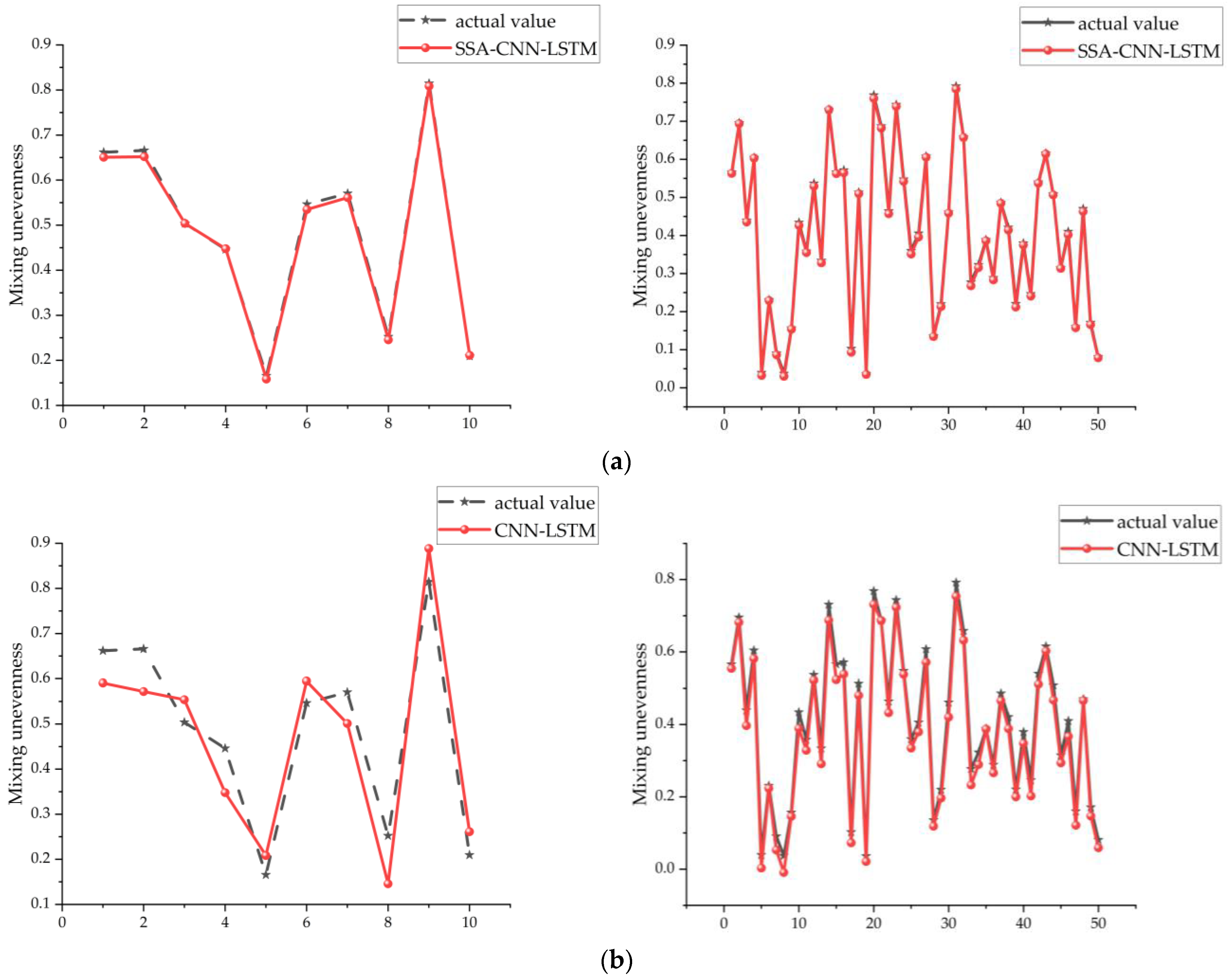
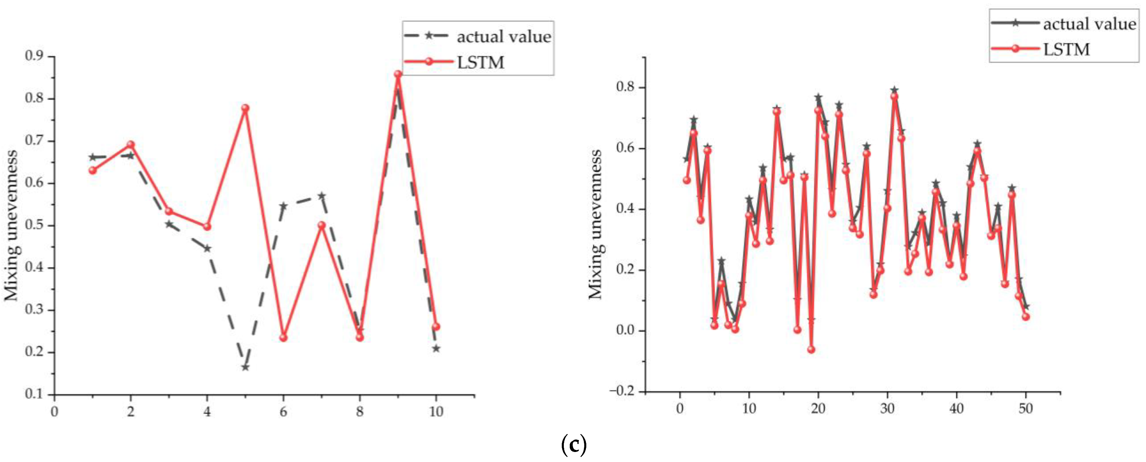
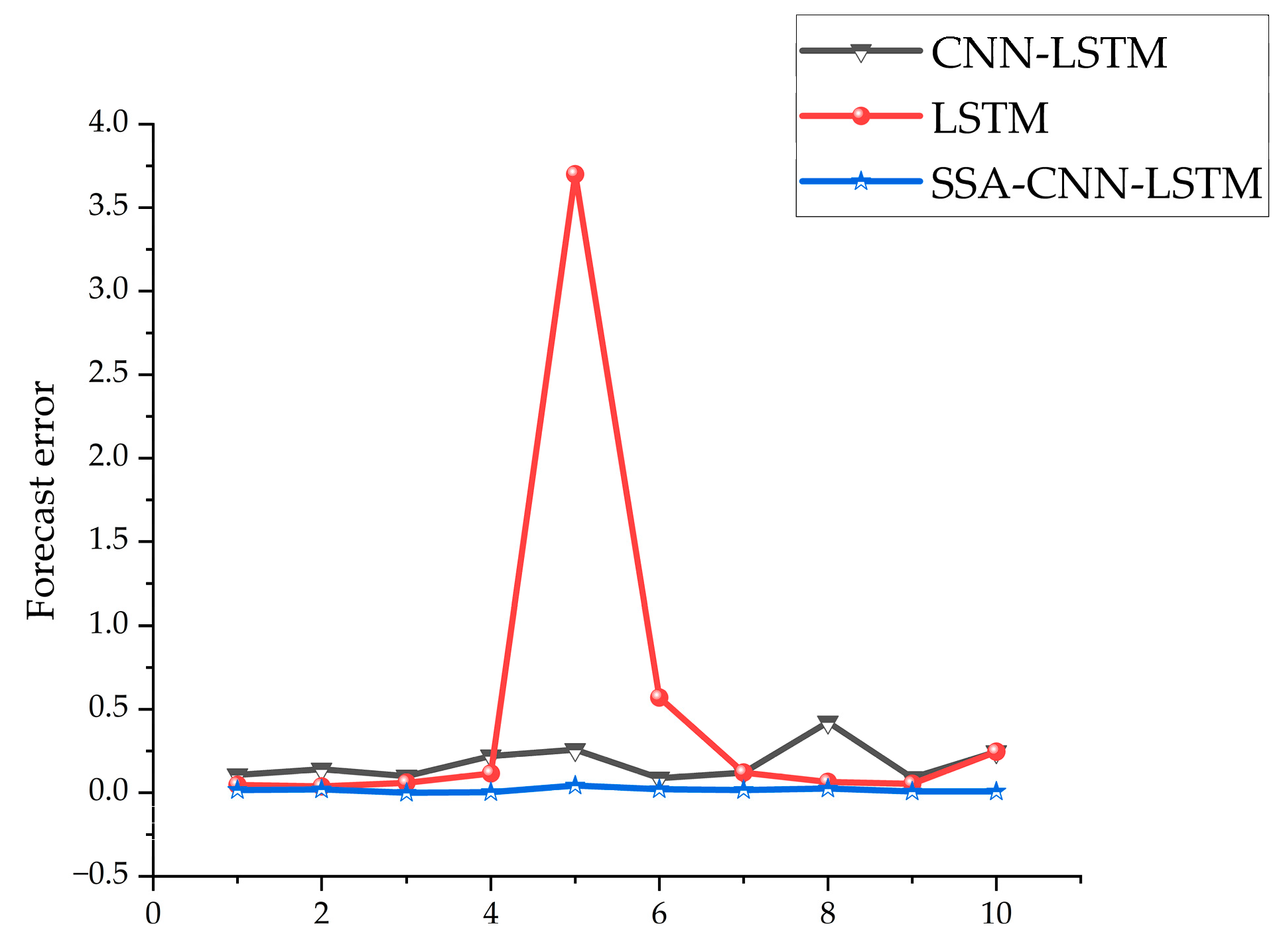
Five sixths of the data from the chosen sample database were used as training data, with the remaining serving as the test set. The predictive performance and prediction errors of various algorithms are shown in Figure 14 and Figure 15, respectively. It can be observed from the figures that SSA-CNN-LSTM has the smallest prediction error, not exceeding 2%, followed by CNN-LSTM, with LSTM showing the poorest predictive performance. In the experiment, the prediction indicators were inlet diameter, outlet diameter, and angle of attack. The SSA optimized three parameters for CNN-LSTM: the optimal number of neurons was set at 75, the optimal initial learning rate at 0.006258, and the optimal L2 regularization coefficient at 0.0004562. By comparing the actual values and predicted values, it can be seen that SSA-CNN-LSTM fits better than various baseline models.

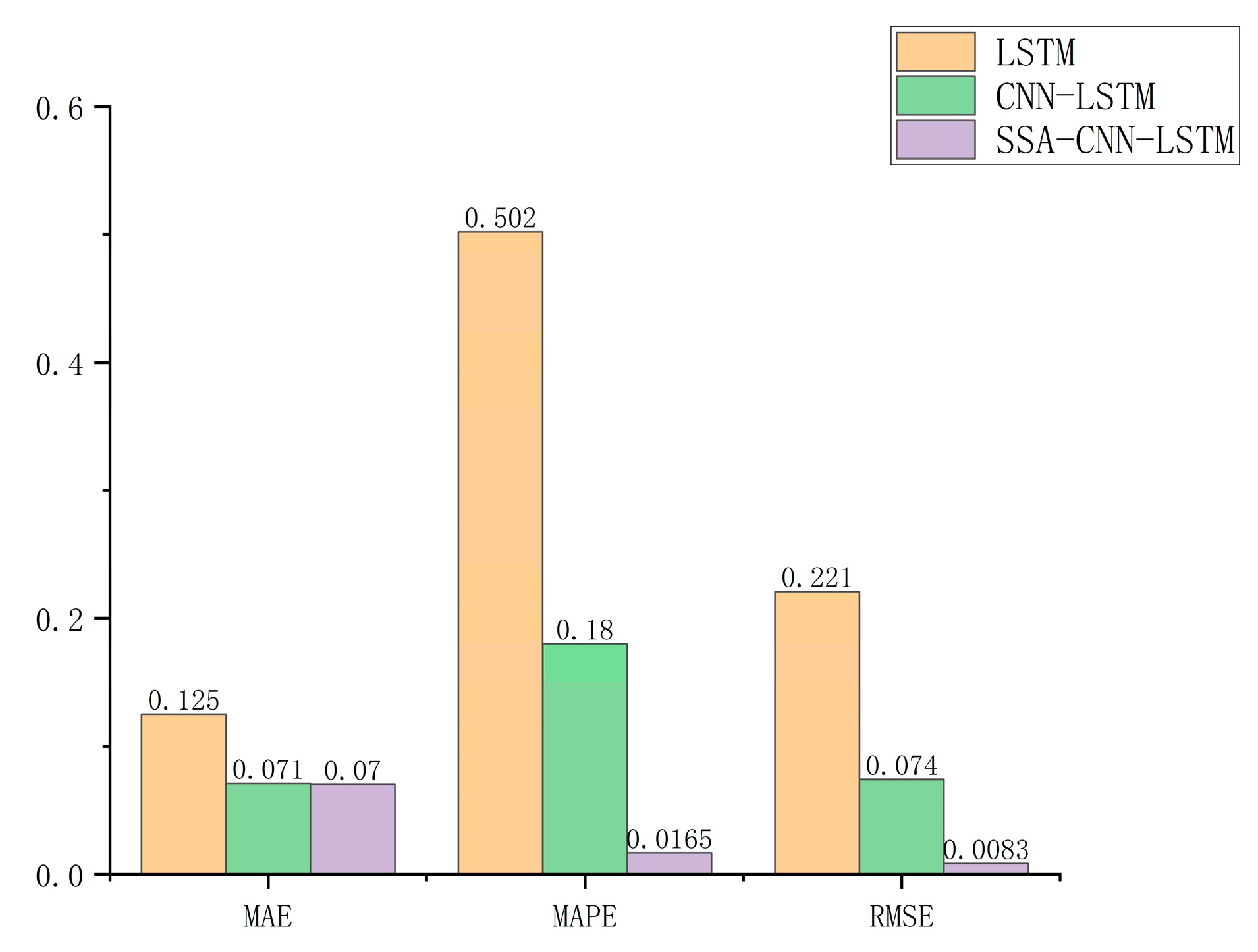
The prediction results of the above three algorithms were statistically analyzed, and as shown in

Table 5. Predictive indicator values of various algorithms.

Method	MAE	MAPE	RMSE
LSTM	0.125	0.502	0.221
CNN-LSTM	0.071	0.18	0.074
SSA-CNN-LSTM	0.07	0.0165	0.0083

and Figure 16, SSA-CNN-LSTM achieved the best results according to the evaluation metrics RMSE, MAE, and MAPE. MAPE was reduced from 12.5% to 7%, achieving an accuracy improvement of 44 percentage points. RMSE and MAE also decreased, indicating that the model’s predictive performance had improved following optimization.

4.4. Joint Optimization Design of SSA-CNN-LSTM and the WOA

The WOA is a relatively novel optimization algorithm proposed in recent years. In 2016, Mirjalili et al. [30] from Griffith University in Australia introduced the WOA, inspired by the unique predatory behavior of humpback whales observed in the ocean. As an emerging swarm intelligence optimization algorithm, the WOA is characterized by its few parameters, simple structure, and high flexibility. Specifically, the advantages are as follows:

(1)

The algorithm’s optimization mechanism is primarily controlled by a random number (Pa), a threshold parameter (A), and a random number (C), resulting in fewer control parameters.

(2)

The WOA is divided into three main optimization mechanisms, with a relatively simple formula model that is easy to implement.

(3)

The WOA offers high flexibility, as it can switch between optimization mechanisms using the random number (Pa) and the threshold parameter (A).

As a result, the WOA can be widely applied in various engineering fields [31]. For example, Li et al. [32] designed a WOA-based optimization algorithm for evaluating bipolar transistor models. In the field of intelligent healthcare, Hassan et al. [33] proposed a hybrid algorithm based on the WOA for diagnosing equipment faults. He et al. [34] developed an improved WOA for adaptively searching for optimal parameters in stochastic resonance systems. El-Fergany et al. [35] used the WOA to enhance the accuracy of fuel cell models.

The overall optimization process of the WOA mainly consists of three parts: Encircling Prey, the Bubble-Net Attacking Technique, and Searching for Prey. Through the cooperation of these three processes, the optimization process can achieve good global search capability and accurate and fast local convergence ability. Thus, while ensuring fast convergence of the algorithm, it can also avoid falling into local optimal solutions, ensuring that the obtained optimal solution is the global optimum, fully leveraging the best performance of the optimization algorithm.

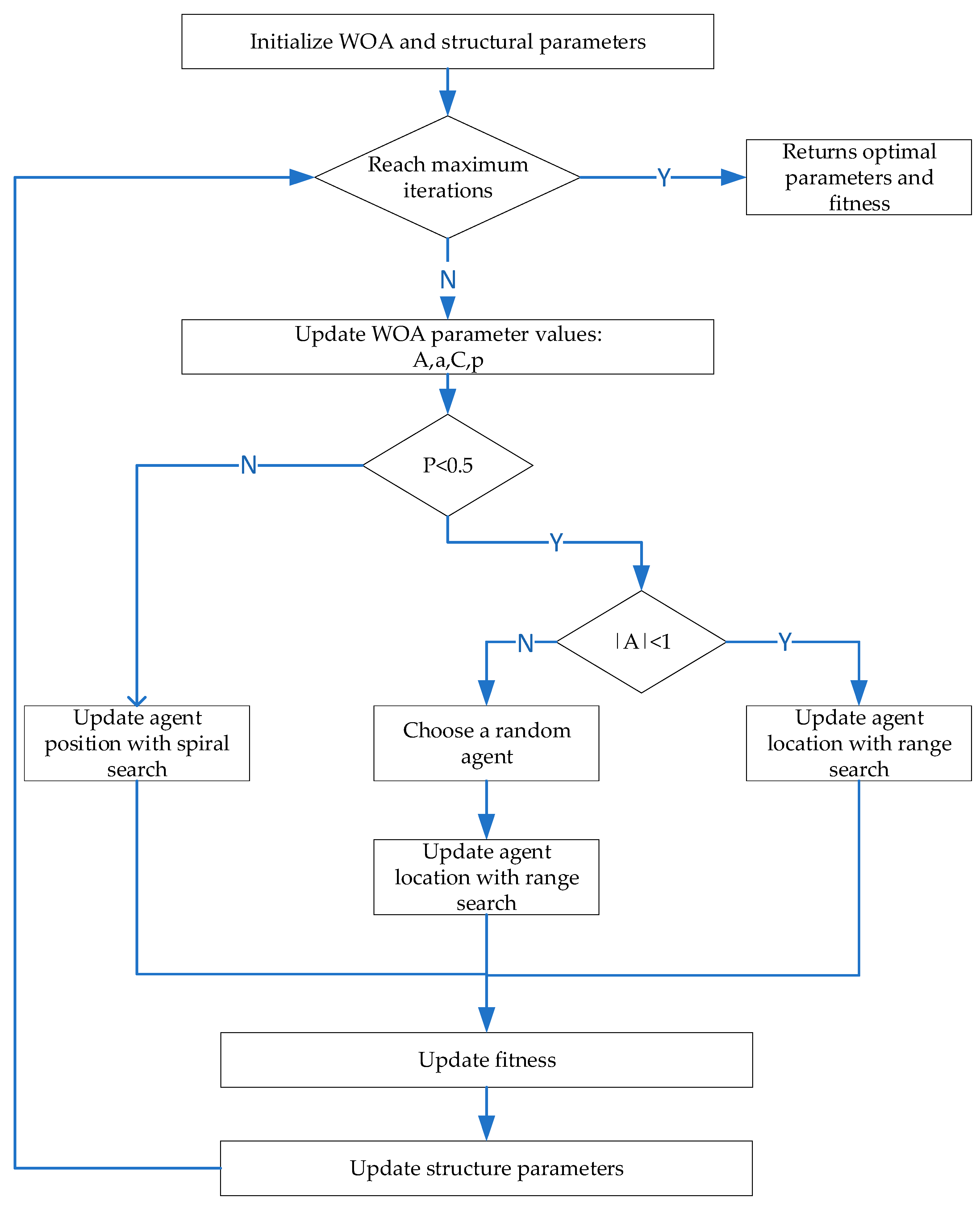
The optimization process of the WOA is as follows: First, initialize the WOA parameter values and input the structural parameters to be optimized. At the beginning of each iteration, check if the maximum number of iterations has been reached. If it has, return the current best structural parameter values and their corresponding fitness values. If the maximum number of iterations has not been reached, update the WOA parameters (A, a, C, and Pa).

The search strategy is then determined based on the random number (p): If Pa < 0.5, further check the value of |A|. If |A| < 1, select a random agent and update its position using the range search mechanism; otherwise, update the search agent’s position using the spiral search strategy. Next, calculate the new fitness value for each search agent and update the structural parameters based on these fitness values. This process repeats until the maximum number of iterations is achieved. Finally, when the maximum number of iterations is reached, the algorithm returns the best structural parameter values and their corresponding fitness values.

Based on the above algorithm steps, the flowchart of the WOA is illustrated as shown in Figure 17.

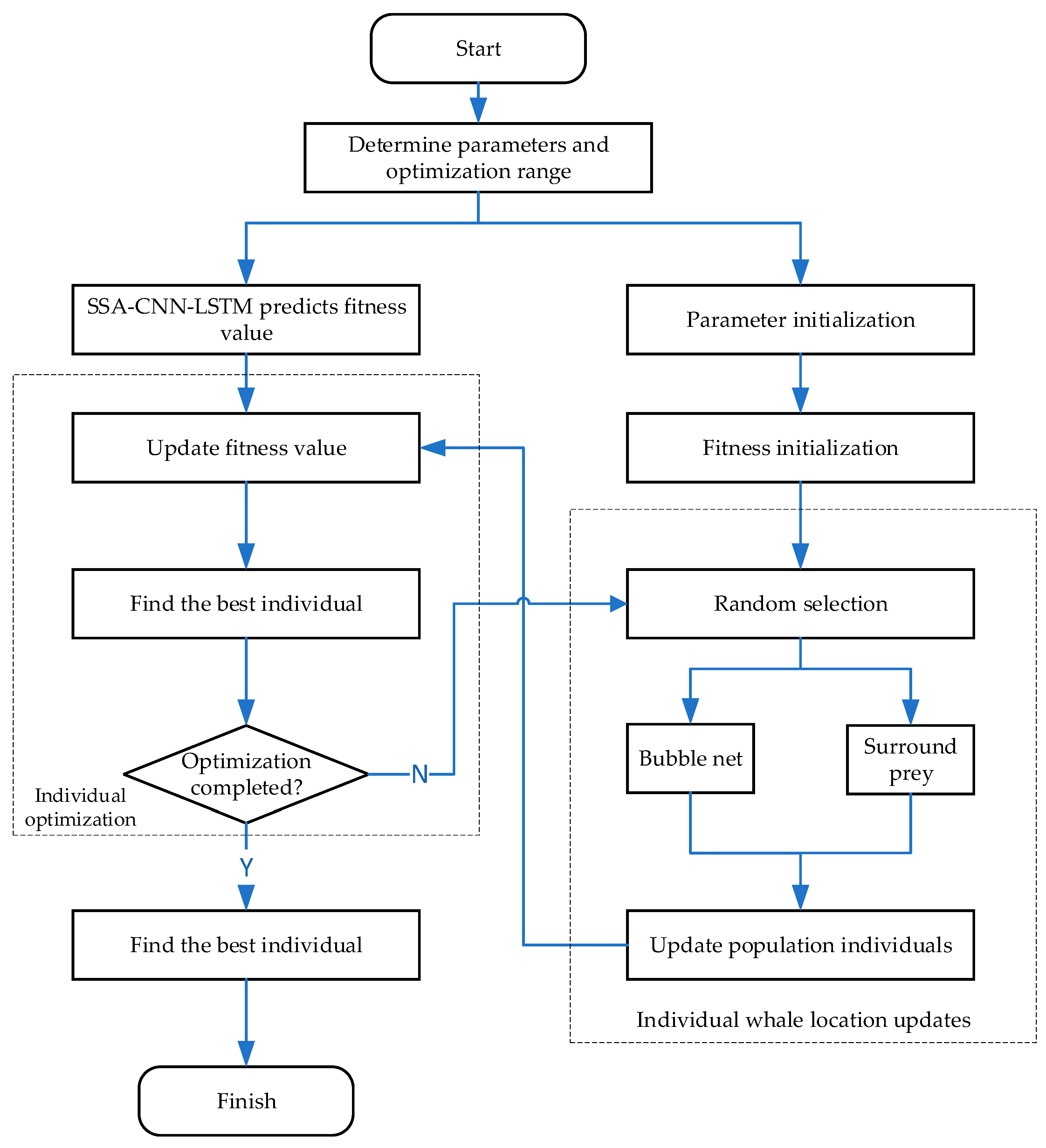
Based on the information provided, the combined optimization algorithm of SSA-CNN-LSTM and the WOA can rapidly optimize structural parameters. Utilizing the determined structural model, an SSA-CNN-LSTM prediction model is built from the sample library to establish a functional relationship between structural parameters and their corresponding fitness values. This enables the input of parameter values to yield fitness values as outputs. After determining the optimization range of parameter values, the parameters of the optimization algorithm are initialized. The SSA-CNN-LSTM model determines the fitness value of each individual in each generation, facilitating selection and iteration, ultimately obtaining the best parameter values and outputting the optimal solution with its corresponding fitness value. Compared to traditional optimization methods, the combined algorithm offers higher efficiency, achieving superior optimization accuracy and better results in a shorter time. The combined optimization process of SSA-CNN-LSTM and the WOA is illustrated in Figure 18.

The prediction output of the trained model is used as the individual fitness value, eliminating individuals with inferior fitness values in favor of superior ones. The WOA is utilized to globally optimize the search for extrema in the prediction model. To demonstrate the superior capabilities of the WOA, it is compared with traditional genetic algorithms and particle swarm optimization.

The Particle Swarm Optimization (PSO) algorithm initializes a swarm of particles within the feasible solution space, characterizing each particle by its position, velocity, and fitness. As the particles move, they update their positions using the individual best position—Pbest—the position with the optimal fitness value experienced by the particle—and the global best position—Gbest—the position with the optimal fitness value found by all particles in the swarm. Pbest and Gbest positions are continuously updated by comparing and adjusting fitness values [36].

The Genetic Algorithm (GA) [37] follows Darwin’s theory of survival of the fittest and simulates biological gene inheritance. The GA calculates a fitness function to evaluate the quality of individuals in the population, classifying them based on these values. Inferior individuals are eliminated, while superior ones survive. This iterative process ensures that the best individuals are passed on to subsequent generations, eventually leading to a population containing the optimal individuals [38,39].

The optimization performance is highlighted by comparing optimization times and the optimization effects of the best fitness values. The results are shown in Figure 19. From the figure, it can be seen that the GA requires 303 iterations to obtain the optimal parameter values, PSO also requires 41 iterations to achieve the optimal parameter values, while the WOA only needs 17 steps to obtain the best optimization solution. At the same time, compared with the GA and PSO, the WOA yields better optimization results. According to the previous text, the lower the mixing unevenness achieved, the better the performance. Here, combined with Figure 4, Figure 5, Figure 6, Figure 7, Figure 8, Figure 9, Figure 10, Figure 11 and Figure 12, it can be observed that the best solutions obtained by the GA, PSO, and WOA are 0.039, 0.037, and 0.03, respectively. Through comparison, it can be seen that the WOA has a faster optimization speed and can achieve better optimization results with fewer iterations. After optimization by the WOA, the best structural parameters obtained are: inlet diameter of 7, outlet diameter of 31.6, and impingement angle of 119.5°.

5. CFD Validation Results

After optimization using SSA-CNN-LSTM-WOA, we compared the density distribution at the mixer outlet and the flow conditions within the mixer before and after the optimization. This comparison was conducted to verify the effectiveness of the optimization.

5.1. The Density Distribution at the Outlet after Optimization

Based on the WOA optimization results, three parameters were adjusted in 3D drawing software. The obtained structural parameters will be subjected to simulation calculations. The optimized outlet cross-section density cloud image and corresponding density data were obtained and calculate the mixing unevenness, which was found to be 0.031. Figure 20 displays the density cloud image post-optimization. There is a significant difference in the density distribution before and after optimization; initially, it was more concentrated, whereas, post-optimization, the density distribution is noticeably more uniform compared to the original model. As illustrated in

Table 6. Optimization result.

Structure	D1 [mm]	D2 [mm]	θ [°]	S
Original Structure	8	35	180	0.11
Joint Algorithm Optimization	7	31.6	119.5	0.031
Reduction in Mixture Non-Uniformity				70%
Prediction error				3.1%

, the pre-optimization mixing unevenness was 0.11. Following WOA optimization, this value decreased to 0.031, a reduction of 70%. Comparing this with the predicted mixing unevenness in MATLAB, the error margin is 3.1%, demonstrating the stability of the SSA-CNN-LSTM prediction. Additionally, the mixing effect of the mixer has been enhanced to some extent after the WOA optimization.

5.2. Velocity Distribution before and after Optimization

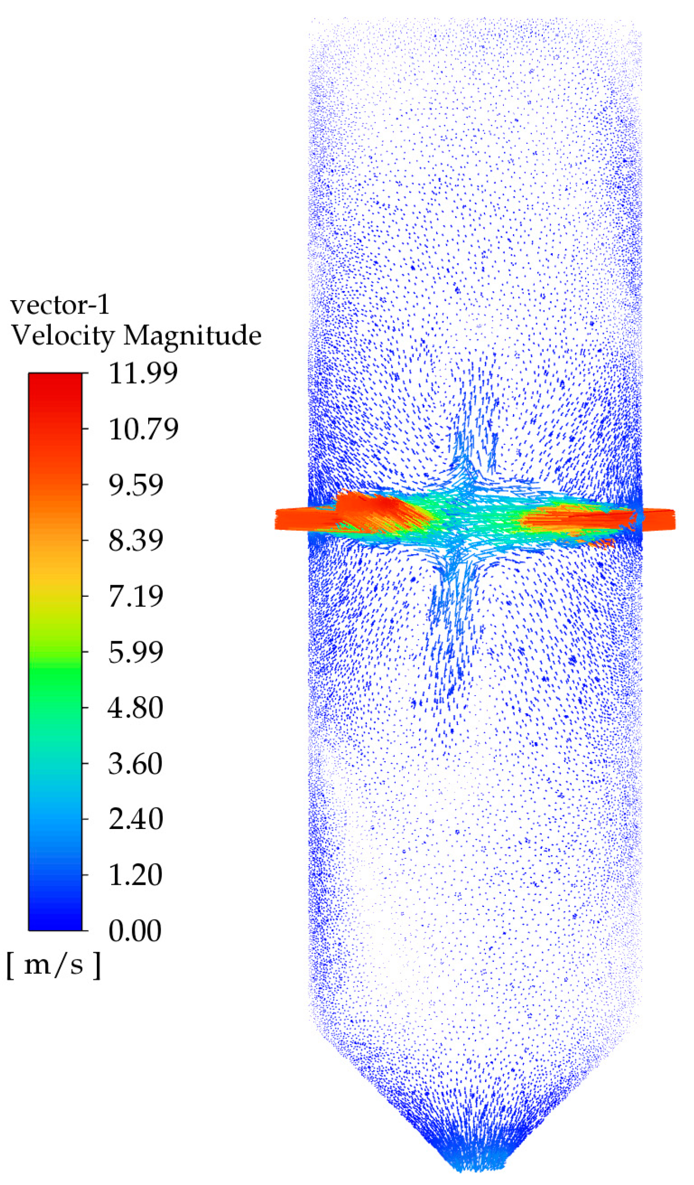
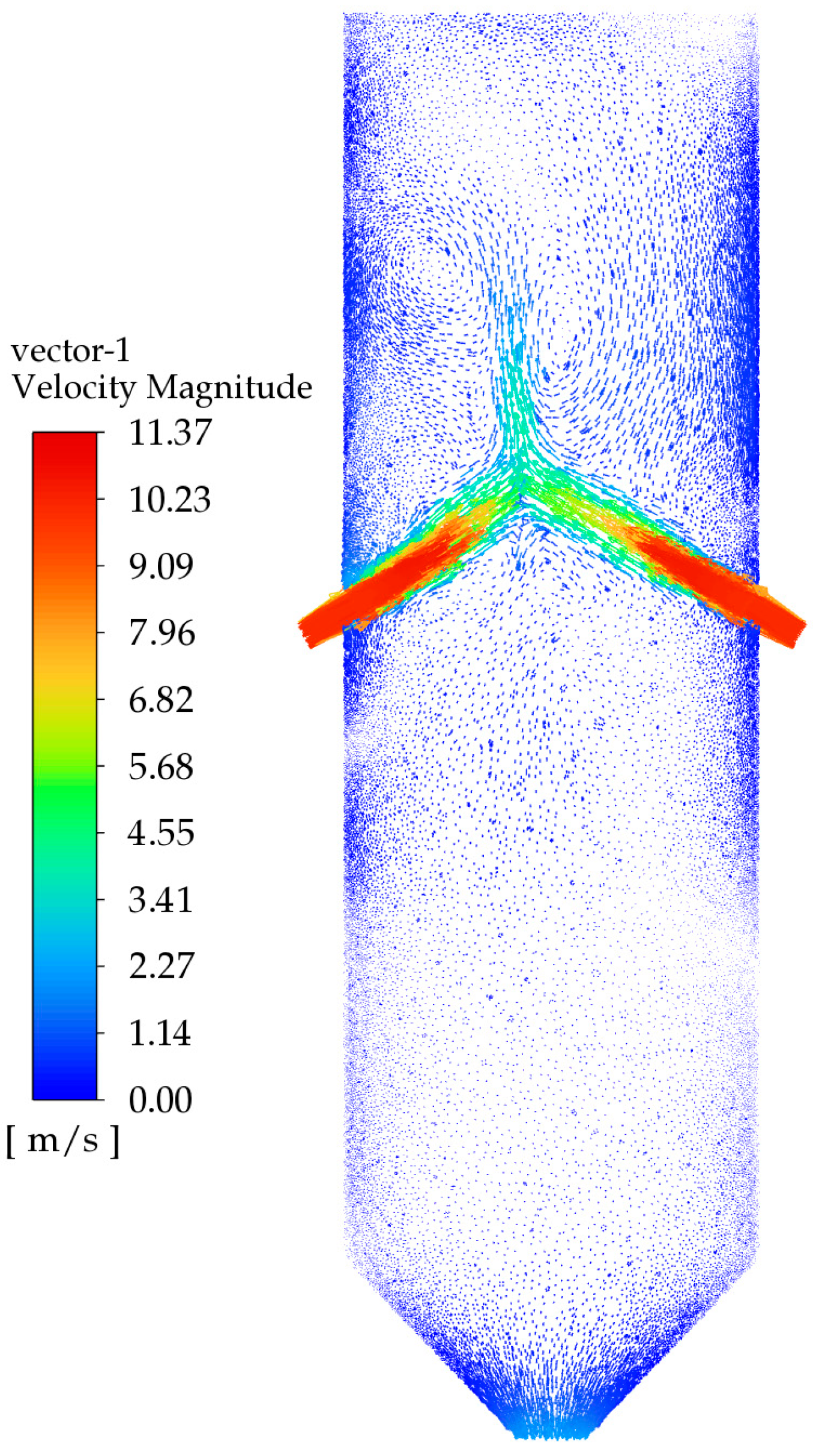
Figure 21 shows the velocity vector diagram before optimization. As seen in the figure, due to the excessive impingement angle, the liquid’s velocity decreases sharply after collision, almost no vortices are generated, and the high-speed region is concentrated. The velocity gradient is significant, and the liquid almost exits the mixer without hitting the walls, resulting in poor mixing. Figure 22 shows the velocity vector diagram after optimization using the joint optimization algorithm. The figure illustrates that the two materials collide at a certain angle, resulting in less velocity loss compared to the original mixer, and generating a certain number of vortices, which improves the mixing effect. Additionally, Figure 22 indicates that the velocity changes smoothly at the intersection, with the velocity vectors being more uniform and the velocity gradient being smaller. Based on the analysis of the velocity changes and vortex structures, it can be concluded that the flow characteristics within the optimized mixer are more conducive to mixing compared to the original mixer.

6. Conclusions

In this study, the analysis of the current high-pressure mixier is executed and an optimal design framework is proposed. Firstly, the most important parameters that distinctly influence mixing unevenness are selected by using the full factorial DOE. Afterward, we constructed an SSA-CNN-LSTM prediction model and used the WOA algorithm to determined the best parameter set. The verification is achieved in the CFD simulation and the detailed conclusions are as follows:

(1)

The structural parameters that obviously influence mixing unevenness are mixer outlet diameter, impingement angle, inlet diameter, and impingement pressure, ranked in order of decreasing importance.

(2)

An SSA-CNN-LSTM prediction model achieves a prediction accuracy of up to 98%, which is higher than the LSTM neural network and CNN-LSTM models. Meanwhile, the SSA demonstrated its superior optimization and convergence capabilities to determine the optimal parameters faster and accurately.

(3)

A joint optimization framework based on SSA-CNN-LSTM and the WOA is proposed to obtain the best parameter set. Based on the optimized mixer parameter values, the mixing unevenness decreases by 70%, significantly enhancing the mixer’s performance.

References

1. Li, E.; Yu, X.; Fan, L.; Xu, Y.; Liu, W. Development of PI Films with Active Groups. Insul. Mater. 2011, 44, 12–15. [Google Scholar]
2. Deng, S.; Wang, J.; Yang, W. Simulation and Analysis of High-Pressure High-Speed Collision Process in Fluid Inside Mixing Head of Reinforced Reaction Injection Molding Machine. China Plast. 2022, 36, 130–136. [Google Scholar]
3. Pei, K.; Li, R.; Zhu, Z. Effects of geometry and process conditions on mixing behavior of a multijet mixer. Ind. Eng. Chem. Res. 2014, 53, 10700–10706. [Google Scholar] [CrossRef]
4. Zhan, X.; Jing, D. Influence of geometric parameters on the fluidic and mixing characteristics of T-shaped micromixer. Micro Syst. Technol.-Micro Nano Syst.-Inf. Storage Process. Syst. 2020, 26, 2989–2996. [Google Scholar] [CrossRef]
5. Yuan, X.; Liao, Y. Analysis of Material Flow Field in the Mixer of Polyurethane Foaming Machine. J. Wuhan Inst. Technol. 2006, 28, 67–69. [Google Scholar]
6. Trautmann, P.; Piesche, M. Experimental investigations on the mixing behavior of impingement mixers for polyurethane production. Chem. Eng. Technol. 2001, 24, 1193–1197. [Google Scholar] [CrossRef]
7. Guo, M. Research on Key Technologies of Polymer Road Repair Foaming Machine; Wuhan Institute of Technology: Wuhan, China, 2011. [Google Scholar]
8. Schneider, F.W. High Pressure Impingement Mixing Apparatus. U.S. Patent 4440500, 3 April 1984. [Google Scholar]
9. Bayer, A.G. Apparatus for the Continuous Preparation of a Liquid Reaction Mixture from Two Fluid Reactants. U.S. Patent 5093084, 3 March 1992. [Google Scholar]
10. Murphy, S.A.; Meszena, Z.G.; Johnson, A.F. Experimental and modelling studies with mixers for potential use with fast polymerisations in tubular reactors. Polym. React. Eng. 2001, 9, 227–247. [Google Scholar] [CrossRef]
11. van Horn, I.B. Venturi Mixer. U.S. Patent 3507626, 21 April 1970. [Google Scholar]
12. Pan, Y. Research on Performance Optimization and Internal Flow Characteristics of Centrifugal Pumps Based on Particle Swarm Optimization Algorithm; Jiangsu University: Zhenjiang, China, 2022. [Google Scholar]
13. Jiang, D.; Zhou, P.; Wang, L.; Wu, D.; Mou, J. Analysis of the Impeller Optimization Design for Dual-Blade Sewage Pumps Based on Response Surface Methodology. J. Hydroelectr. Eng. 2021, 40, 72–82. [Google Scholar]
14. Luo, M.; Zuo, Z.; Li, H.; Li, W.; Chen, H. Multi-objective Optimization Design Method for Centrifugal Compressor Impellers Based on BP Neural Network. J. Aerosp. Power 2016, 31, 2424–2431. [Google Scholar]
15. Jiang, M.; Mei, Y.; Luo, Y.; Yu, S.; Hu, D. Structural Parameter Optimization of the Mixing Head of Polyurethane Foaming Machine Based on GA-BP-GA. Eng. Plast. Appl. 2023, 12, 92–99. [Google Scholar]
16. Li, L.; Guo, Z.; Liu, Y.; Li, P. Numerical Simulation and Structural Optimization of Supersonic Spray Nozzles. J. Dalian Jiaotong Univ. 2023, 3, 58–62. [Google Scholar] [CrossRef]
17. Liu, G.; Zhao, T.; Wang, C.; Yang, Z.; Yang, X.; Li, S. Optimization of Structure and Operating Parameters of Y-Type Micromixers in Two-Phase Pulsatile Mixing. J. Jilin Univ. (Eng. Technol. Ed.) 2015, 45, 1155–1161. [Google Scholar]
18. Guo, D. Parameter Optimization and Flow Field Characteristics Study of a New Type of Impinging Stream Reactor; Taiyuan University of Technology: Taiyuan, China, 2020. [Google Scholar]
19. Dai, B. Modular Design and Research of Polyurethane Foaming Equipment; Soochow University: Suzhou, China, 2020. [Google Scholar]
20. Zhang, J.; Niu, J.; Dong, X.; Feng, Y. Numerical Simulation of the Flow Field in an Impinging Stream Reactor and the Optimization of Its Mixing Performance. Chin. J. Process Eng. 2022, 22, 1244–1252. [Google Scholar]
21. Zhang, J.; Shang, P.; Yan, J.; Feng, Y. Mixing Effects of a Horizontal Opposed Bidirectional Impinging Stream Mixer. Chin. J. Process Eng. 2017, 17, 959–964. [Google Scholar]
22. Palanisamy, B.; Paul, B. Continuous flow synthesis of ceria nano particles using static T-mixers. Chem. Eng. Sci. 2012, 78, 46–52. [Google Scholar] [CrossRef]
23. Niu, J. Numerical Simulation Analysis of the Flow Field in an Impinging Stream Reactor and Research on the Preparation of Calcium Hydroxide Nano Powder; Shenyang University of Chemical Technology: Shenyang, China, 2022. [Google Scholar]
24. Zhengyang, Z.; Zhuo, C.; Hongjie, Y.; Liu, F.; Liu, L.; Cui, Z.; Shen, D. Numerical simulation of gas—Liquid multi-phase flows in oxygen enriched bottom-blown furnace. Chin. J. Nonferrous Met. 2012, 22, 1826–1834. [Google Scholar]
25. Wenli, L.; Yanbing, Y.; Dongming, Z.; Feng, M. Water modeling on double porous plugs bottom blowing in a 150t ladle. Jiangxi Metall. 2022, 42, 1–9. [Google Scholar] [CrossRef]
26. Wang, D.X.; Liu, Y.; Zhang, M.; Li, X.-L. PIv measurements on physical models of bottom blown oxygen smelting furnace. Can. Metall. Copp. Q. 2017, 56, 221–231. [Google Scholar] [CrossRef]
27. Zhang, G.; Zhu, R. Modeling and on-Hne optimization control memod of oxygen bottom-blowing copper smelting process. China Nonferrous Metall. 2020, 49, 62–65. [Google Scholar]
28. Xue, W.; Liang, Y. Efficient hydraulic and thermal simulation model of the multi-phase natural gas production system with variable speed compressors. Appl. Therm. Eng. 2024, 242, 122411. [Google Scholar] [CrossRef]
29. Ji, N.; Zhang, W.; Yu, Y.; He, Y.; Hou, Y. Multi-Objective Optimization of Injection Molding Based on Optimal Latin Hypercube Sampling Method and NSGA–II Algorithm. Eng. Plast. Appl. 2020, 48, 72–77. [Google Scholar]
30. Mirjalili, S.; Lewis, A. The whale optimization algorithm. Adv. Eng. Softw. 2016, 95, 51–67. [Google Scholar] [CrossRef]
31. Tu, J.; Chen, H.; Liu, J.; Heidari, A.A.; Zhang, X.; Wang, M.; Ruby, R.; Pham, Q.V. Evolutionary biogeography-based whale optimization methods with communication structure: Towards measuring the balance. Knowl. Based Syst. 2021, 21, 212–240. [Google Scholar] [CrossRef]
32. Li, L.L.; Sun, I.; Tseng, M.L.; Zhi-Gang, L. Extreme learning machine optimized by whale optimization algorithm using insulated gate bipolar transistor module aging degree evaluation. Expert Syst. Appl. 2019, 127, 58–67. [Google Scholar] [CrossRef]
33. Hassan, M.K.; El Desouky, A.I.; Elghamrawy, S.M.; Sarhan, A.M. A hybrid real-time remote monitoring framework with NB-WOA algorithm for patients with chronic Diseases. Future Gener. Comput. Syst. 2019, 93, 77–95. [Google Scholar] [CrossRef]
34. He, B.; Huang, Y.; Wang, D.; Yan, B.; Dong, D. A parameter-adaptive stochastic resonance based on whale optimization algorithm for weak signal detection for rotating machinery. Meas. J. Int. Meas. Confed. 2019, 136, 658–667. [Google Scholar] [CrossRef]
35. El-Fergany, A.A.; Hasanien, H.M.; Agwa, A.M. Semi-empirical PEM fuel cells model using whale optimization algorithm. Energy Convers. Manag. 2019, 201, 112–127. [Google Scholar] [CrossRef]
36. Run, X.; Zuo, Y.; Huo, D. Optimal design of truss structure based on pso algorithm. Steel Constr. 2012, 27, 37–39. [Google Scholar]
37. Michalewicz, Z.; Janikow, C.Z.; Krawczyk, J.B. A modified genetic algorithm for optimal control problems. Comput. Math. Appl. 1992, 23, 83–94. [Google Scholar] [CrossRef]
38. Wang, G.; Chen, Y.; Li, Q.; Lu, C.; Chen, G.; Huang, L. Ultrasonic computerized tomography imaging method with combinatorial optimization algorithm for concrete pile foundation. IEEE Access 2019, 7, 132395–132405. [Google Scholar] [CrossRef]
39. Wang, L.; Zheng, C. Identification method of aerodynamic damping based on the genetic algorithm and random decrement technique. J. Vib. Shock. 2023, 42, 16–23. [Google Scholar]
Figure 1. High-pressure mixer.
Actuators 13 00303 g001
Figure 2. High-pressure-mixer three-dimensional model.
Actuators 13 00303 g002
Figure 3. Mesh independence verification.
Actuators 13 00303 g003
Figure 4. Mesh division results.
Actuators 13 00303 g004
Figure 5. Distribution of sampling points.
Actuators 13 00303 g005
Figure 6. Original mixer head outlet section density contour.
Actuators 13 00303 g006
Figure 7. Pareto chart of standardization effect.
Actuators 13 00303 g007
Figure 8. SSA-CNN-LSTM-WOA optimization process.
Actuators 13 00303 g008
Figure 9. OLH sampling results.
Actuators 13 00303 g009
Figure 10. LHS sampling results.
Actuators 13 00303 g010
Figure 11. Sampling space.
Actuators 13 00303 g011
Figure 12. Schematic diagram of the SSA-CNN-LSTM model.
Actuators 13 00303 g012
Figure 13. SSA-CNN-LSTM model flowchart.
Actuators 13 00303 g013
Figure 14. (a). SSA-CNN-LSTM prediction results. (b). CNN-LSTM prediction results. (c). LSTM prediction results.
Actuators 13 00303 g014aActuators 13 00303 g014b
Figure 15. Prediction errors of various algorithms.
Actuators 13 00303 g015
Figure 16. Comparison chart of evaluation indicators.
Actuators 13 00303 g016
Figure 17. WOA process.
Actuators 13 00303 g017
Figure 18. SSA-CNN-LSTM-WOA joint optimization process.
Actuators 13 00303 g018
Figure 19. The fitness curve.
Actuators 13 00303 g019
Figure 20. Density distribution of the exit cross-section after WOA optimization.
Actuators 13 00303 g020
Figure 21. Velocity vector diagram before optimization.
Actuators 13 00303 g021
Figure 22. Velocity streamline diagram after optimization.
Actuators 13 00303 g022