All articles published by MDPI are made immediately available worldwide under an open access license. No special
permission is required to reuse all or part of the article published by MDPI, including figures and tables. For
articles published under an open access Creative Common CC BY license, any part of the article may be reused without
permission provided that the original article is clearly cited. For more information, please refer to
https://www.mdpi.com/openaccess.
Feature papers represent the most advanced research with significant potential for high impact in the field. A Feature
Paper should be a substantial original Article that involves several techniques or approaches, provides an outlook for
future research directions and describes possible research applications.
Feature papers are submitted upon individual invitation or recommendation by the scientific editors and must receive
positive feedback from the reviewers.
Editor’s Choice articles are based on recommendations by the scientific editors of MDPI journals from around the world.
Editors select a small number of articles recently published in the journal that they believe will be particularly
interesting to readers, or important in the respective research area. The aim is to provide a snapshot of some of the
most exciting work published in the various research areas of the journal.
This paper investigates decentralized adaptive event-triggered fault-tolerant control for interconnected nonlinear delay systems with actuator failures. The actuator failures suffered include loss of effectiveness and bias faults. A control scheme based on the K-filter is proposed, which effectively compensates for the effects of unknown actuator failures. A hyperbolic tangent function and neural network are introduced to approximate the unknown interconnection function and nonlinear delay function. By introducing the dynamic surface control method, the “explosion of complexity” issue is addressed. Furthermore, our proposed controller can ensure that all states of the corresponding closed-loop system are semi-globally uniformly ultimately bounded and that the tracking error can converge to a small neighborhood of zero. Meanwhile, Zeno behavior can be effectively avoided. Finally, the validity of the proposed control scheme is verified using a simulation example.
In recent years, adaptive control for nonlinear systems has been widely studied. Because neural networks (NNs) and fuzzy logic systems (FLSs) have strong approximation ability, they are used to approximate unknown nonlinear functions. As typical nonlinear systems, interconnected nonlinear systems are popular because of their broad application. Interconnected nonlinear systems have nonlinear and uncertain characteristics, which lead to difficulties in controller design. To address these problems, a decentralized control structure has been proposed, which naturally reduces the computational burden associated with centralized control. Hence, some researchers have proposed some adaptive decentralized control methods for interconnected nonlinear systems [1,2]. In [3], an adaptive decentralized control method for interconnected nonlinear systems with unmodeled dynamics was proposed. The adaptive fuzzy decentralized output-feedback control problem for switched interconnected nonlinear systems was first investigated in [4]. A decentralized backstepping control method for interconnected systems with non-triangular structural uncertainties was investigated in [5]. In practice, time-varying delay characteristics are common, significantly impacting the stability and performance of the system. The traditional linear theory cannot describe and deal with these delay characteristics. To address this issue, an adaptive decentralized control method based on NNs for interconnected nonlinear systems with time delays was proposed in [6]. The decentralized output-feedback control problem for interconnected nonlinear systems with input delays and saturation was studied in [7].
The occurrence of actuator failures is common in modern industrial control systems, which affects the stability of the system. Consequently, it is of great theoretical and practical significance to study fault-tolerant control (FTC) of nonlinear systems [8,9]. In recent years, many effective FTC methods have been developed to address the above-mentioned problems. In [10], an adaptive fuzzy fault-tolerant control method was proposed for the cascade chemical reactor system. In [11,12], adaptive FTC methods were developed for a class of single-input single-output (SISO) nonlinear systems. In the existing literature [13,14,15,16], the focus has gradually shifted from SISO nonlinear systems to multi-input multiple-output (MIMO) nonlinear systems with the same actuator failures mentioned in [11,12]. It can be seen that the above works are based on continuous control methods to address the control problem of nonlinear systems with actuator failures, including loss of effectiveness and bias faults. However, few researchers have addressed the control problem of interconnected nonlinear delay systems with such actuator failures using the discrete control method.
In recent years, event-triggered control has become a research hotspot. Compared with the continuous control method, event-triggered control can save limited communication bandwidth while ensuring system performance. As a result, event-triggered control has been extensively studied. In [17], the adaptive event-triggered control problem for a class of uncertain nonlinear systems was considered, in which the assumption of the input-to-state stability is no longer needed. In [18], an adaptive NN event-triggered control method for switched nonlinear systems was proposed, in which the restrictions on nonlinear functions no longer need to be considered. In [19], the adaptive event-triggered control problem for a more general nonlinear system was considered, considering cases with unmodeled dynamics and nonlinear time delays. Furthermore, the authors of [20] proposed an encoding–decoding mechanism that further saves communication resources based on an event-triggered mechanism. As far as we know, event-triggered control has good flexibility and responsiveness, helping to reduce wear and failure to a certain extent. Nevertheless, constructing an event-triggered controller for interconnected nonlinear systems with actuator faults remains a challenge. Therefore, this issue becomes the second motivation for this study.
Based on the above discussion, this paper investigates the output-feedback adaptive event-triggered tracking control problem for a class of uncertain nonlinear large-scale interconnected systems with actuator failures and time-varying delays. Although the above-mentioned articles have been well studied, addressing the coupling problem between the interconnection and time-varying delay components becomes important. Moreover, effectively saving communication resources and designing a decentralized adaptive event-triggered fault-tolerant control scheme under the premise of ensuring system performance is particularly important. The main contributions of this paper can be summarized as follows:
Compared with the literature [13,14,21,22], a new fault-tolerant control strategy based on the K-filter is proposed. The unmeasured states are well estimated, and the actuator failures are compensated for. The interconnected nonlinear function and nonlinear delay function are approximated by introducing a hyperbolic tangent function and NNs.
A decentralized adaptive event-triggered controller is developed to ensure that all closed-loop signals are bounded and that tracking errors can converge to a small neighborhood of zero. Furthermore, by utilizing dynamic surface control and backstepping technology, the “explosion of complexity” issue is addressed.
Compared with the continuous control method [4,5,7], our proposed event-triggered control method can effectively reduce communication resources. It is proven through theoretical analysis that the Zeno phenomenon is avoided.
This paper is organized as follows. Problem description and preliminaries are provided in Section 2. In Section 3, the state observer, and the decentralized event-triggered controller are designed, and the system stability is analyzed. In Section 4, simulation results are shown. Conclusions are presented in Section 5.
Notations: ℜ denotes the set of real numbers; denotes the -dimensional Euclidean space; and denotes the real matrix space. is usually the symbol used to denote the expected value or expected absolute value in mathematics.
2. Problem Description and Preliminaries
In this paper, we consider the following interconnected nonlinear delay systems with actuator failures in the form of:
where ; ; and ; ; and are the unmeasurable system states, control input with actuator failure, and output of the i-th subsystem, respectively. is an unknown parameter, and with is known as the smooth function vector. is the unknown smooth nonlinear interconnected function vector, where and represent and , respectively. is the unknown smooth time-varying nonlinear delay function vector, where represents , and is the time-varying delay function. Here, and .
Actuator failures with loss of effectiveness and bias faults can be modeled as
where is the output of the i-th local actuator; is our designed input; is the unknown actuator efficiency factor satisfying ; and is the uncertain bounded bias function.
Definition1.
Consider the following nonlinear system:
The trajectory of system (3) is said to be semi-globally uniformly ultimately bounded (SGUUB) at the p-th moment if for some compact set and any initial state , there exists a constant , and a time constant such that for all . When , it is usually called SGUUB in the mean square.
Our control objective is to develop a decentralized adaptive event-triggered output-feedback controller in the form of (67) for system (1) with actuator faults (2) such that all states of the resulting closed-loop system are SGUUB and the tracking error can converge to a small neighborhood of zero.
To achieve the objective, some assumptions and lemmas are given below.
Assumption1.
The desired trajectories and are available and bounded for .
Assumption2
([23]).For , , the interconnected nonlinear function satisfies
where denotes the unknown smooth function.
Assumption3
([24]).The nonlinear functions satisfy the following inequalities for
where and are positive constants. represents the uncertain smooth function, where for , , . Additionally, satisfies
where and are variables, represents the uncertain functions, and represents the bounded functions for a bounded variable with .
Lemma1
([25]).There exists a constant and a variable such that
Lemma2
([26]).Define the set , . For , the inequality holds, where is a constant.
Lemma3
([27]).For the continuous function on the compact set , a radial basis function neural network (NN) exists such that
where is the ideal weight vector and , with being the Gaussian function. The number of NN nodes is , and is the bounded approximation error with .
Lemma4.
For any constant and any variable , the following inequality holds
3. Main Results
In this section, the main results are presented. First, a K-filter is constructed to estimate the unmeasured states. Then, the intermediate design steps are given. Subsequently, a decentralized event-triggered controller is designed. Finally, the system stability is analyzed.
3.1. State Observer Design
To obtain the unmeasurable states, we design a K-filter utilizing the output signal and control signal for the i-th subsystem
where such that all the eigenvalues of are in the open left-half plane; ; and is the same as in (2). Then, the state estimate of the i-th subsystem for system (1) can be expressed as
Remark1.
On the one hand, the K-filter based on actuator failures is constructed to address the coupling problem of unknown states and actuator effectiveness loss. On the other hand, the K-filter updates the state estimates recursively, avoiding redundant calculations and improving computational efficiency.
The observer error is defined as . Its derivative is
For the error system, we consider the following Lyapunov function
where is a positive definite matrix such that , with being a positive definite matrix to be determined in stability analysis.
Then, taking the time derivative of along (14), one has
Using Young’s inequality, one can obtain the following equalities:
Substituting (17), (18), and (19) into (16) yields
3.2. Intermediate Design Steps
Let , , , and denote the second entries of , , , and , respectively. Based on the design procedure similar to [28], we have
Then, we formulate the following coordinate changes:
where represents the output of the first-order low-pass filters. These filters for , are described as follows:
where is a design parameter.
Remark2.
In the backstepping control approach, the design of the control law involves the utilization of states as virtual control signals. Each step of the design necessitates both the virtual control signals and their corresponding derivatives. Theoretically, the calculation of the virtual control signal derivatives is simple. However, it can be quite complicated and tedious in applications when n is greater than three because the control signal will include the derivative of , the second derivative of , and the third derivative of , thereby causing the “explosion of complexity” problem. To address this problem, a dynamic surface control method was proposed in [29,30,31].
Define the difference between the virtual controller and the first-order low-pass filter as follows:
Remark3.
According to [32], the boundary layer errors will converge asymptotically to zero only if is very small. Thus, we should set to a small constant in the simulation example. Additionally, the boundedness of is guaranteed by introducing the boundary layer error.
Concerning the unknown parameters, we introduce
where and are the estimations of and , respectively. and are the corresponding estimation errors.
where denotes the estimation of , with , and is a design parameter.
The time derivative of can be obtained as follows:
where .
According to Young’s inequality and Assumption 2, one has
where for are smooth nonlinear functions.
Then, one can have
Choose the Lyapunov candidate function as
where and is a design parameter, whose time derivative is
where we define .
Let . Then, the derivative of can be obtained as follows:
where .
Next, the unknown nonlinear delay functions and interconnection terms in the Lyapunov function are approximated using NNs.
According to Assumption 3 and Young’s inequality, one has
Let . According to Lemma 3, we can obtain , where .
Remark4.
According to Assumptions 2 and 3, both the interconnected nonlinear function and the time-vary nonlinear function can be represented by smooth functions about . Therefore, in this paper, we choose to eliminate the influence of the interconnected nonlinear function and time-varying nonlinear function in the first step related to and approximate the nonlinear function using NNs.
Using Young’s inequality, one has
Construct the stabilizing function as follows:
where is a positive design parameter. With the aid of Lemma 4, we obtain
Choose the virtual control signal and adaptive laws as follows:
where is a design parameter.
Remark5.
The K-filter based on actuator failures is constructed, which draws attention to the effect of actuator failures when constructing the -th virtual controller. This makes it difficult for us to construct a virtual controller. The stabilizing function and an adaptive law are introduced to address the problem of actuator failures.
The dynamics of the boundary layer error are given as follows:
In this section, an event-triggered controller is designed to stabilize interconnected nonlinear delay systems with actuator failures. On the premise of maintaining system performance, unnecessary communication resources are reduced.
The local actual control law and event-triggered mechanism are designed as follows:
where is an intermediate continuous control law, which is given later; denotes the measurement error; and and are design parameters.
According to the above event-triggered mechanism, holds all the time. When and satisfy and , respectively, we obtain
with and satisfying
where is any number in .
The control protocol and adaptive law are designed as follows:
3.4. Stability Analysis and Avoidance of Zeno Behavior
For the stability analysis, we choose the total Lyapunov function V as .
Theorem1.
Consider a closed-loop system consisting of interconnected nonlinear systems (1); actuator failures (2); the K-filter (10)–(12); the adaptive controller designed in (45), (55), (61), and (67); and the event-triggered mechanisms (63)–(64). Then, all the signals in the closed-loop system are SGUUB, and the tracking error can converge to a small neighborhood of zero. Additionally, Zeno behavior can be effectively avoided.
Proofof Theorem 1.
As , then and . Since and , one has
According to Lemma 1, the following inequality can be obtained:
Substituting (65) and (70) into (62), we can obtain
According to (51), (57), and (71), differentiating V yields
The following inequalities are established by choosing an appropriate positive definite matrix , , and for
where and are parameters, and , , and .
According to Lemma 2, for ; For , with being a constant. In conclusion, for convenience, with for .
Then, adopting Young’s inequalities yields
where , , and . Therefore, following a similar analysis to [21], all the closed-loop signals are SGUUB.
From (75), we obtain that . As a result, , , , , and are also bounded.
As , and is bounded, is bounded. Since is Hurwitz, and are bounded. From the backstepping procedure, and are bounded. By following a similar analysis to [33], system (1) is rephrased as
Because and are bounded and is Hurwitz, is bounded. As a result, all the closed-loop signals are bounded.
Now, we show that the proposed controller can avoid Zeno behavior, i.e., for the i-th subsystem, there exists a positive number such that . Since , , one has
From (61) and (67), is differentiable, and is a function consisting of all the bounded closed-loop signals. Therefore, there exists a constant such that . Since and , it is obtained that the lower bound of must satisfy . Therefore, Zeno behavior is avoided. □
4. Simulation Example
In this section, a simulation example is provided to verify the theoretical result. We consider interconnected nonlinear delay systems with actuator failures. The system model is given by
where and are unknown constants, but they are set as and .
The nonlinear functions in (78) are given as , , , , , , , , , and , where are the time-varying delay functions.
The initial values of the variables are given as , , , , , , , , , , , , and . Then, is the basis function vector, with being the Gaussian function in the following form:
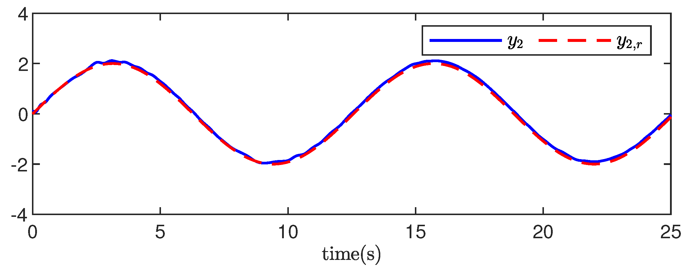
where is the center of the neural network. The desired trajectory signal of each subsystem is chosen as , .
The design parameters are , , , , , , , , , , , , , , , , , and .
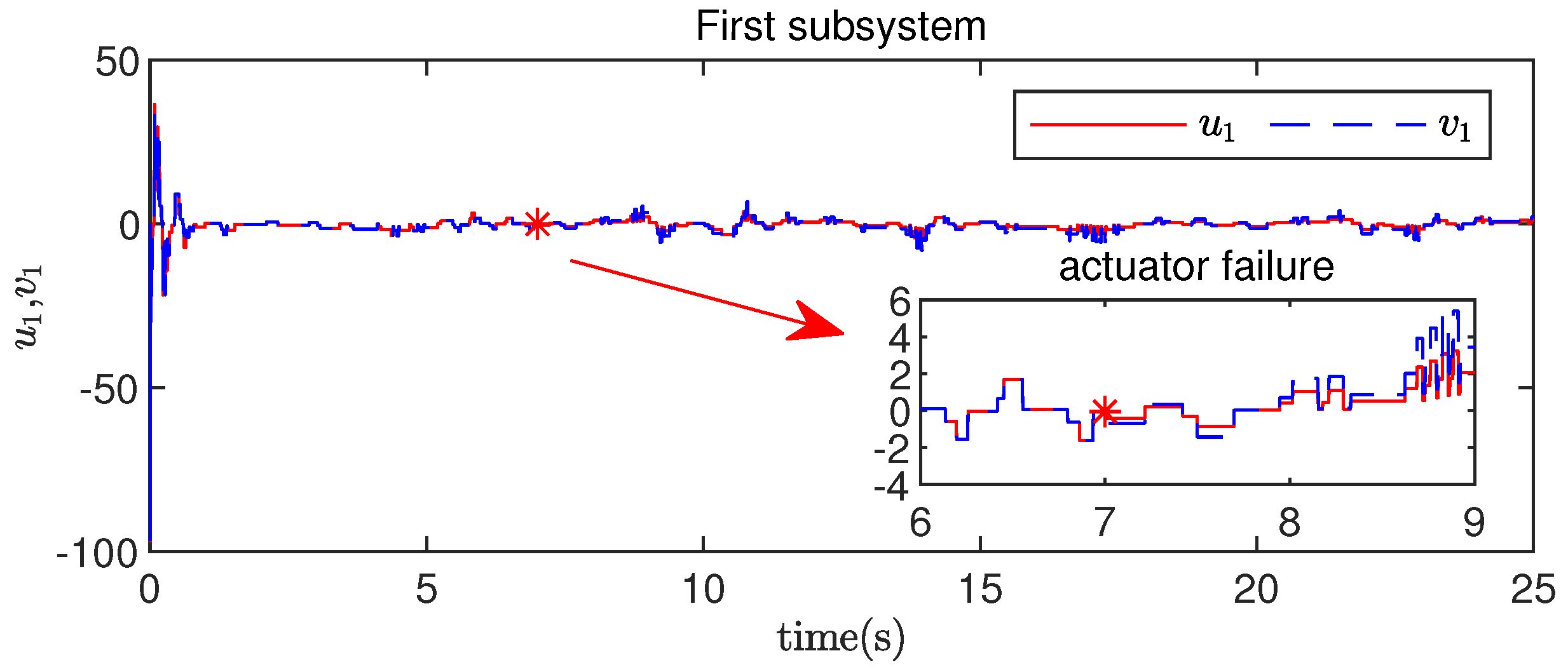
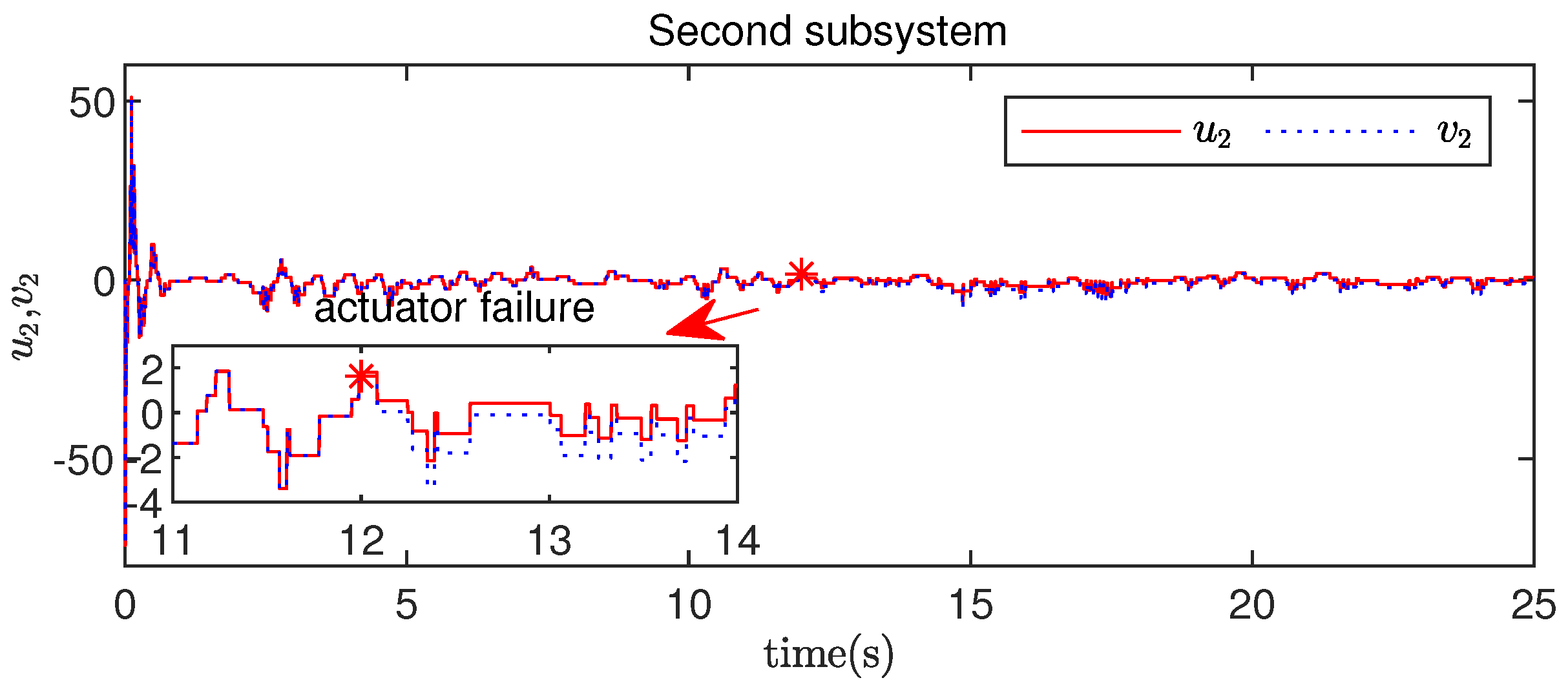
Actuator 1 with loss of effectiveness is described as , s, and actuator 2 with loss of effectiveness and bias faults is described as , s. Based on the above analysis, the verification results are given in Figure 1, Figure 2, Figure 3, Figure 4 and Figure 5. The output of the two subsystems is given in Figure 1 and Figure 2. Figure 3 and Figure 4 depict the input and output signals of the two actuators. It is worth noting that the moment when the actuator failure occurred is marked with ∗. The time intervals of the triggering events are shown in Figure 5. Obviously, all the closed-loop signals are bounded and Zeno behavior is avoided.
5. Conclusions
In this paper, a decentralized observer-based event-triggered fault-tolerant control scheme was derived for interconnected nonlinear delay systems. Our proposed event-triggered controller ensures that all system states are SGUUB. The problem of the “explosion of complexity” is addressed by introducing first-order low-pass filters. The property of hyperbolic tangent functions and the approximation capability of NNs are used to handle interconnected nonlinear functions and time-varying delays. According to the simulation example, the Zeno phenomenon is avoided. In the future, it would be interesting to study dual-channel event-triggered control for interconnected nonlinear systems with actuator failures and denial-of-service attacks.
Author Contributions
Conceptualization, W.H. and Y.L.; methodology, Y.L.; software, W.H.; validation, Y.L.; formal analysis, Y.L.; investigation, Y.L.; writing—original draft preparation, Y.L.; writing—review and editing, W.H., Y.L., and Q.Z.; supervision, W.H. and Q.Z. All authors have read and agreed to the published version of the manuscript.
Funding
This work was supported in part by the National Key Research and Development Program of China under grant 2022YFB3305300 and in part by the National Natural Science Foundation of China under grant 62333010.
Data Availability Statement
The data presented in this study are available on request from the corresponding author. The data are not publicly available as no datasets were generated or analyzed during the current study.
Conflicts of Interest
The authors declare no conflicts of interest.
References
Ioannou, P. Decentralized adaptive control of interconnected systems. IEEE Trans. Autom. Control1986, 31, 291–298. [Google Scholar] [CrossRef]
Tong, S.; Liu, C.; Li, Y. Fuzzy-Adaptive Decentralized Output-Feedback Control for Large-Scale Nonlinear Systems with Dynamical Uncertainties. IEEE Trans. Fuzzy Syst.2010, 18, 845–861. [Google Scholar] [CrossRef]
Tong, S.; Zhang, L.; Li, Y. Observed-Based Adaptive Fuzzy Decentralized Tracking Control for Switched Uncertain Nonlinear Large-Scale Systems with Dead Zones. IEEE Trans. Syst. Man Cybern. Syst.2016, 46, 37–47. [Google Scholar] [CrossRef]
Cai, J.; Wen, C.; Xing, L.; Yan, Q. Decentralized Backstepping Control for Interconnected Systems with Non-Triangular Structural Uncertainties. IEEE Trans. Autom. Control2023, 68, 1692–1699. [Google Scholar] [CrossRef]
Tong, S.; Li, Y.; Zhang, H. Adaptive Neural Network Decentralized Backstepping Output-Feedback Control for Nonlinear Large-Scale Systems with Time Delays. IEEE Trans. Neural Netw.2011, 22, 1073–1086. [Google Scholar] [CrossRef] [PubMed]
Li, Y.; Chen, B.; Lin, C.; Shang, Y. Adaptive neural decentralized output-feedback control for nonlinear large-scale systems with input time-varying delay and saturation. Neurocomputing2021, 427, 212–224. [Google Scholar] [CrossRef]
Su, Y.; Jiang, Y.; Tong, M.; Wang, H. Predefined Time and Accuracy Adaptive Fault-Tolerant Control for Nonlinear Systems with Multiple Faults. Actuators2024, 13, 131. [Google Scholar] [CrossRef]
Cui, G.; Bao, C.; Guo, M.; Xu, Y.; He, Y.; Wu, J. Research on Path Tracking Fault-Tolerant Control Strategy for Intelligent Commercial Vehicles Based on Brake Actuator Failure. Actuators2024, 13, 97. [Google Scholar] [CrossRef]
Liu, X.; Wang, Y.; Chen, D.; Chen, H. Adaptive fuzzy fault-tolerant control for a class of unknown non-linear dynamical systems. IET Control Theory Appl.2016, 10, 2357–2369. [Google Scholar] [CrossRef]
Li, Y.; Yang, G. Adaptive asymptotic tracking control of uncertain nonlinear systems with input quantization and actuator faults. Automatica2016, 72, 177–185. [Google Scholar] [CrossRef]
Wang, Y.; Xu, N.; Liu, Y.; Zhao, X. Adaptive fault-tolerant control for switched nonlinear systems based on command filter technique. Appl. Math. Comput.2021, 392. [Google Scholar] [CrossRef]
Tong, S.; Huo, B.; Li, Y. Observer-Based Adaptive Decentralized Fuzzy Fault-Tolerant Control of Nonlinear Large-Scale Systems with Actuator Failures. IEEE Trans. Fuzzy Syst.2013, 22, 1–15. [Google Scholar] [CrossRef]
Wang, C.; Wen, C.; Lin, Y. Decentralized adaptive backstepping control for a class of interconnected nonlinear systems with unknown actuator failures. J. Frankl. Inst.2015, 352, 835–850. [Google Scholar] [CrossRef]
Wang, C.; Wen, C.; Guo, L. Decentralized output-feedback adaptive control for a class of interconnected nonlinear systems with unknown actuator failures. Automatica2016, 71, 187–196. [Google Scholar] [CrossRef]
Li, Y.; Yang, G. Adaptive Fuzzy Decentralized Control for a Class of Large-Scale Nonlinear Systems with Actuator Faults and Unknown Dead Zones. IEEE Trans. Syst. Man Cybern. Syst.2017, 47, 729–740. [Google Scholar] [CrossRef]
Xing, L.; Wen, C.; Liu, Z.; Su, H.; Cai, J. Event-Triggered Adaptive Control for a Class of Uncertain Nonlinear Systems. IEEE Trans. Autom. Control2017, 64, 2071–2076. [Google Scholar] [CrossRef]
Li, S.; Ahn, C.; Guo, J.; Xiang, Z. Neural-Network Approximation-Based Adaptive Periodic Event-Triggered Output-Feedback Control of Switched Nonlinear Systems. IEEE T. Cybern.2020, 51, 4011–4020. [Google Scholar] [CrossRef] [PubMed]
Li, M.; Li, S.; Ahn, C.; Xiang, Z. Adaptive Fuzzy Event-Triggered Command-Filtered Control for Nonlinear Time-Delay Systems. IEEE Trans. Fuzzy Syst.2022, 30, 1025–1035. [Google Scholar] [CrossRef]
Xing, L.; Wen, C.; Liu, Z.; Su, H.; Cai, J. Event-Triggered Output Feedback Control for a Class of Uncertain Nonlinear Systems. IEEE Trans. Autom. Control2019, 64, 290–297. [Google Scholar] [CrossRef]
Xu, L.; Wang, Y.; Wang, X.; Peng, C. Decentralized event-triggered adaptive control for interconnected nonlinear systems with actuator failures. IEEE Trans. Fuzzy Syst.2022, 31, 148–159. [Google Scholar] [CrossRef]
Choi, Y.; Yoo, S. Event-triggered decentralized adaptive fault-tolerant control of uncertain interconnected nonlinear systems with actuator failures. ISA Trans.2018, 77, 77–89. [Google Scholar] [CrossRef] [PubMed]
Chen, X.; Li, S.; Wang, R.; Xiang, Z. Event-Triggered output feedback adaptive control for nonlinear switched interconnected systems with unknown control coefficients. Appl. Math. Comput.2023, 445, 127854. [Google Scholar] [CrossRef]
Hua, C.; Liu, G.; Li, L.; Guan, X. Adaptive Fuzzy Prescribed Performance Control for Nonlinear Switched Time-Delay Systems with Unmodeled Dynamics. IEEE Trans. Fuzzy Syst.2018, 26, 1934–1945. [Google Scholar] [CrossRef]
Song, X.; Sun, P.; Ahn, C.; Song, S. Switching ETM-based neural adaptive output feedback control for nonaffine stochastic MIMO nonlinear systems subject to deferred constraint. Neural Netw.2023, 167, 668–679. [Google Scholar] [CrossRef] [PubMed]
Wang, Z.; Yuan, Y.; Yang, H. Adaptive Fuzzy Tracking Control for Strict-Feedback Markov Jumping Nonlinear Systems with Actuator Failures and Unmodeled Dynamics. IEEE Trans. Cybern.2018, 50, 126–139. [Google Scholar] [CrossRef]
Gao, Z.; Liu, D.; Zhou, Z. Fault tolerant control scheme for a class of interconnected nonlinear time delay systems using event-triggered approach. IEEE Access2020, 8, 162730–162747. [Google Scholar] [CrossRef]
Swaroop, D.; Hedrick, J.; Yip, P.; Gerdes, J. Dynamic surface control for a class of nonlinear systems. IEEE Trans. Autom. Control2000, 45, 1893–1899. [Google Scholar] [CrossRef]
Wang, D.; Huang, J. Neural network-based adaptive dynamic surface control for a class of uncertain nonlinear systems in strict-feedback form. IEEE Trans. Autom. Control2005, 16, 195–202. [Google Scholar] [CrossRef]
Zang, T.; Ge, S. Adaptive dynamic surface control of nonlinear systems with unknown dead zone in pure feedback form. Automatica2008, 44, 1895–1903. [Google Scholar] [CrossRef]
Cheng, T.; Niu, B.; Zhang, J.; Wang, D.; Wang, Z. Time-/Event-Triggered Adaptive Neural Asymptotic Tracking Control of Nonlinear Interconnected Systems with Unmodeled Dynamics and Prescribed Performance. IEEE Trans. Neural Netw. Learn. Syst.2023, 34, 6557–6567. [Google Scholar] [CrossRef] [PubMed]
Zhang, L.; Deng, C.; Che, W.; An, L. Adaptive backstepping control for nonlinear interconnected systems with prespecified-performance-driven output triggering. Automatica2023, 154, 111063. [Google Scholar] [CrossRef]
Figure 1.
The output of the first subsystem.
Figure 1.
The output of the first subsystem.
Figure 2.
The output of the second subsystem.
Figure 2.
The output of the second subsystem.
Figure 3.
Input and output signals of actuator 1.
Figure 3.
Input and output signals of actuator 1.
Figure 4.
Input and output signals of actuator 2.
Figure 4.
Input and output signals of actuator 2.
Figure 5.
Time intervals of triggering events.
Figure 5.
Time intervals of triggering events.
Disclaimer/Publisher’s Note: The statements, opinions and data contained in all publications are solely those of the individual author(s) and contributor(s) and not of MDPI and/or the editor(s). MDPI and/or the editor(s) disclaim responsibility for any injury to people or property resulting from any ideas, methods, instructions or products referred to in the content.
He, W.; Liu, Y.; Zhang, Q.
Decentralized Output-Feedback Adaptive Event-Triggered Control for Interconnected Nonlinear Delay Systems with Actuator Failures. Actuators2024, 13, 188.
https://doi.org/10.3390/act13050188
AMA Style
He W, Liu Y, Zhang Q.
Decentralized Output-Feedback Adaptive Event-Triggered Control for Interconnected Nonlinear Delay Systems with Actuator Failures. Actuators. 2024; 13(5):188.
https://doi.org/10.3390/act13050188
Chicago/Turabian Style
He, Wenmin, Yu Liu, and Quanling Zhang.
2024. "Decentralized Output-Feedback Adaptive Event-Triggered Control for Interconnected Nonlinear Delay Systems with Actuator Failures" Actuators 13, no. 5: 188.
https://doi.org/10.3390/act13050188
APA Style
He, W., Liu, Y., & Zhang, Q.
(2024). Decentralized Output-Feedback Adaptive Event-Triggered Control for Interconnected Nonlinear Delay Systems with Actuator Failures. Actuators, 13(5), 188.
https://doi.org/10.3390/act13050188
Note that from the first issue of 2016, this journal uses article numbers instead of page numbers. See further details here.
Article Metrics
No
No
Article Access Statistics
For more information on the journal statistics, click here.
Multiple requests from the same IP address are counted as one view.
He, W.; Liu, Y.; Zhang, Q.
Decentralized Output-Feedback Adaptive Event-Triggered Control for Interconnected Nonlinear Delay Systems with Actuator Failures. Actuators2024, 13, 188.
https://doi.org/10.3390/act13050188
AMA Style
He W, Liu Y, Zhang Q.
Decentralized Output-Feedback Adaptive Event-Triggered Control for Interconnected Nonlinear Delay Systems with Actuator Failures. Actuators. 2024; 13(5):188.
https://doi.org/10.3390/act13050188
Chicago/Turabian Style
He, Wenmin, Yu Liu, and Quanling Zhang.
2024. "Decentralized Output-Feedback Adaptive Event-Triggered Control for Interconnected Nonlinear Delay Systems with Actuator Failures" Actuators 13, no. 5: 188.
https://doi.org/10.3390/act13050188
APA Style
He, W., Liu, Y., & Zhang, Q.
(2024). Decentralized Output-Feedback Adaptive Event-Triggered Control for Interconnected Nonlinear Delay Systems with Actuator Failures. Actuators, 13(5), 188.
https://doi.org/10.3390/act13050188
Note that from the first issue of 2016, this journal uses article numbers instead of page numbers. See further details here.

