Abstract
This study proposes a universal adaptive control algorithm for an unknown multi-input multi-output (MIMO) system using recursive least squares (RLS) and parameter self-tuning. The issue of adjusting the control and system parameters in response to changes in the platform was discussed. The development of a control algorithm that can consistently achieve reliable and robust control performance in various systems is important. This study aimed to develop a control algorithm that can track the reference value for any unknown MIMO system. For the controller design, an nth-order differential error dynamic model was designed, and an RLS with a scale factor was used to estimate the coefficients of the error dynamics. In the current scenario, the numbers of control inputs and error states in the error dynamics were assumed to be equal. It was designed such that the control input is derived based on the Lyapunov stability concept using the estimated coefficients. The scale factor in the RLS and injection term in the control input based on the sliding-mode approach were computed using a self-tuning methodology. The performance of the proposed universal adaptive control algorithm was evaluated using an actual DC motor and CarMaker (version 8.1.1) software tests under various scenarios.
1. Introduction
With the advancement in technology in various platforms, such as autonomous driving mobility, there is an increasing demand for the control of multiple actuators. In recent years, these systems have provided assistance to users; however, in future, automatic control is expected to be replaced by automated functions because of their autonomy while performing different activities. However, to achieve this, accurate knowledge of the system parameters and sophisticated sensors are required because the system parameters affect the control performance. These sensors are expensive and require control to track target values without sensors. In addition, modification of the controller with respect to the variation in the number of actuators or platforms is extremely inefficient in terms of time. Therefore, regardless of the unknown system, the user requires a control technology that can be applied to various systems and can provide stable control.
Liu et al. proposed a robust controller design method that combines particle swarm optimization and computational methods to control multi-input multi-output (MIMO) systems [1]. Homaeinezhad et al. proposed a methodology that merges backstepping and sliding-mode controls to manage nonlinear loads and parameter changes in MIMO systems [2]. Pongfai et al. proposed a parameter design methodology based on a proportional-integral-derivative (PID)-based adaptive cluster learning process for the optimal control of MIMO systems [3]. Homaeinezhad et al. proposed a Lyapunov-stability-based algorithm as a nonpredictive methodology for designing nonlinear MIMO control systems [4]. Recent studies have proposed adaptive fuzzy controllers based on sliding-mode control methods to control electric mobility, hexacopter drones, and electric wheelchairs [5,6,7]. Huang et al. proposed a robust control system that incorporates design procedures such as back-steps to alleviate the controllability conditions of nonlinear MIMO systems with actuator defects [8]. Thanh et al. proposed a super-twist sliding technique for the finite-time stability of uncertain nonlinear systems using MIMO [9]. Zeghlache et al. demonstrated robust control against wind gusts and external disturbances using the Lyapunov method to stabilize a MIMO system and ensure that the desired signal is accurately controlled [10]. As the aforementioned studies defined a control system limited to motors or vehicles and evaluated the proposed algorithm, it was difficult to apply it to various unknown systems [2,5,7]. This study aims to develop a universal controller for application to various unknown systems. Usman et al. estimated the parameters in real time using an observer with upper- and lower-limit ranges based on the parameters of an actual DC motor [11]. Laid and Boubekeur proposed a model-independent control approach using a hyperlocal model identification method for position control of uncertain and unmodeled DC motors [12]. Mynar et al. proposed an extended Kalman filter-based parameter estimation as a sensorless control methodology for efficient and cost-effective motor control [13]. Jiang et al. developed a model-independent adaptive control algorithm that uses front-and-rear-wheel drive control distribution strategies for autonomous vehicles [14]. Wang et al. developed a model-independent four-wheel steering control algorithm for a four-wheel independent steering vehicle to ensure the steering stability based on the input and output data of the vehicle without using a mathematical model [15]. In addition, Fliess and Join proposed a control methodology to minimize the parameter adjustment process without using a mathematical model with a model-independent intelligent PID control algorithm [16]. Liu et al. used sliding-mode control-based uncertainty. Moreover, as a strategy to secure robust control performance against external disturbances, a position-control algorithm that does not consider the constraints of the mathematical model has been proposed [17]. Moreno Gonzalez et al. proposed the lateral control of a vehicle over a wide speed range [18]. Farhan et al. performed a sensorless current prediction control for a motor by estimating the position and speed of the rotor using an extended Kalman filter [19]. Wang and Wang developed an independent data-driven model without any learning process [20]. Numerous studies have confirmed that researchers are developing control algorithms to ensure steering stability by utilizing the extended Kalman filter for model-independent adaptive controls. To use the Kalman filter or enhanced Kalman filter, other system information such as dynamic parameters may be required. To overcome this problem, this study aims to develop an adaptive control that does not use system information. Zhang et al. used camera-based lane detection and side-error calculations to propose a path-tracking algorithm for intelligent electric vehicles. This algorithm integrated a linear quadratic regulator based on error dynamics and sliding-mode control [21]. Research is also underway to devise path tracking for mobile robots that incorporates the robustness of sliding-mode control [22,23] and the uncertainties and disturbances inherent in mathematical models and parameters and reflects the physical properties of the robot based on the model predictive controller [24,25]. Controllers based on mathematical models that are used for path-tracking autonomous vehicles and robots may have a negative impact on control performance owing to uncertainties in the parameters, mathematical models, and disturbances in various driving situations. Research is currently underway to improve the path-tracking control performance by compensating for the uncertainties and disturbances in the parameters and mathematical models. This is achieved using neural networks and deep reinforcement [26,27,28]. Moudoud et al. used an adaptive sliding-mode controller with a fuzzy logic system to track the trajectory of a mobile robot with uncertainties and disturbances [29]. Aware et al. proposed a two-timescale technique based on sliding-mode control to perform lateral control, in which the system obtains a stable yaw rate and sideslip angle [30]. In previous studies, sliding-mode control was used to develop control algorithms for systems with model uncertainties and disturbances. From the perspective of performance advancement, research is being conducted to improve control performance using fuzzy-logic-based adaptive control, neural networks, and deep reinforcement. In this study, we propose a recursive least square (RLS)-based mathematical model-free control algorithm as a methodology for performing universal-purpose control of unknown systems. The proposed algorithm designs error dynamics based on RLS and estimates the coefficients of error dynamics; therefore, it does not require system information. The control algorithm was designed based on the Lyapunov-stability-based sliding-mode scheme, and the magnitude of the injection term required to derive the control input was self-tuned. The main contributions of this study are summarized as follows:
- (1)
- The proposed algorithm estimates the RLS-based error dynamics coefficients and does not require information regarding the system. Therefore, it can be used as a universal-purpose controller in various unknown systems.
- (2)
- In this study, a virtual test drive simulator, CarMaker, and an actual DC motor platform were used to evaluate the reasonable performance of the proposed universal controller. In the case of the CarMaker-based evaluation, this study attempted to verify the performance of the proposed algorithm in various systems using front-wheel steering vehicles and front-and-rear-wheel steering vehicles.
The remainder of this paper is organized as follows: Section 2 introduces the concept of an adaptive control algorithm using RLS and parameter self-tuning. Section 3 discusses the performance of the proposed algorithm using MATLAB/Simulink (version 2019a), an actual DC motor, and the CarMaker (version 8.1.1) software. Finally, Section 4 and Section 5 present conclusions and future work, respectively.
2. Adaptive Control Algorithm Using RLS and Parameter Self-Tuning
Figure 1 depicts a schematic of the proposed adaptive control algorithm. The control error is calculated using the difference between the tracking reference value and the state of the plant. The calculated error is used in the error dynamics for the RLS-based coefficient estimation. At this stage, the error dynamics assume that the numbers of control inputs and errors are equal. RLS estimates the coefficients () required to derive the adaptive control input and uses the residuals to self-tune the parameters for the injection term of the sliding-mode approach based on the Lyapunov direct method. The adaptive control algorithm, which is designed based on the sliding-mode approach and self-tuning injection, determines the control input.

Figure 1.
Block diagram of the adaptive control algorithm.
2.1. MIMO System Error Dynamics
This study explores systems that can be represented by the following error dynamics.
where denotes the control error and denotes the input, and we assume that the following conditions are satisfied:
- (A1)
- All the control errors have a complex influence on each other.
- (A2)
- At this stage, and the number of control errors and control inputs are the same.
According to assumption (2), the control input of Equation (1) can be expressed as Equation (2). The terms for each of the errors can be expressed in the above equation, along with the weighting coefficient of the error. The error dynamics for a MIMO nth-order system can then be considered as follows:
Because this study considers an unknown MIMO system, the coefficients C and D in Equation (2) are unknown matrices. The C and D values were estimated in real time using the recursive least squares method. The next section describes the coefficient estimation.
2.2. RLS-Based Coefficient Estimation
An RLS method with multiple forgetting factors was used to estimate the coefficients. Depending on the number of multiple inputs and outputs, the relationship function for each equation can be designed as shown in Equation (3). Equations (4)–(7) represent the RLS equations used for the coefficient estimation. In the virtual relationship function, y, ϕ, and θ represent the output, regressor, and estimated value, respectively.
In this study, the cost function V was defined using Equation (5) to design a recursive least squares algorithm with multiple forgetting factors between zero and one. The recursive least squares method with multiple forgetting factors treated in this study was designed with reference to previous research [31].
The estimated value that minimizes the sum of the squares of the residuals, which is the cost function, was calculated. The calculation process is shown in Equation (6).
It should be noted that the optimal gain L was used for the estimation and the covariance matrix P was used for calculating the optimal gain L; during each sampling phase, these were repeatedly updated using a forgetting factor and covariance update factor, as shown in Equation (7).
A covariance update factor with a value of one or more is applied to the covariance matrix in Equation (7) to intentionally increase the variance, further giving more weight to the measurements, and is expressed as Equation (8). The scale factor is calculated and applied using the change in error from , the lower limit of the change in error, to , the upper limit. When the error change is less than the lower limit, the scale factor is applied as the constant value, which is the lower limit of the scale factor. When the change in error is greater than the lower limit, the opposite situation applies.
2.3. Derivation of Control Input Based on the Lyapunov Direct Method
In this study, the Lyapunov direct method was used to ensure the stability of the control algorithm. The defined sub cost function was expressed as to minimize each control error. Each sub cost function () for the error equation of the MIMO system on the left side was organized on the right side.
Equation (10) presents the Lyapunov candidate function and two conditions for the error to converge to zero within a finite time. Weights were applied to the Lyapunov candidate function to adjust the weights for each error.
For asymptotic stability, the rate of change in the Lyapunov candidate function with respect to time must always be negative. Therefore, the Lyapunov derivative is derived with respect to time. The rate of change of error defined in Equation (2) is substituted as in Equation (11).
The control input to converge the error to zero and ensure control stability is designed as shown in Equation (12) using the injection term denoted.
The rate of change in the cost function can be obtained from Equation (13) using Equations (11) and (12). Here, the residual between the actual system value and the estimated value is given by Equation (14). Therefore, Equation (13) is rearranged into Equation (15) using the residual.
By defining the boundary value using Equations (16) and (17), Equation (15) can be expressed as Equation (18). Based on this, Equation (13) can be organized into Equation (19) with a finite-time convergence condition of one:
Because the right-hand sides of Equations (18) and (19) can be assumed to be the same, the magnitude of the injection term is determined accordingly.
Equation (12) can be expressed as Equation (21) using the magnitude of the injection term derived from Equation (20). The control input generates unrealistic chattering, depending on the sign of the error. Therefore, to obtain a continuous control signal, the discontinuous function was replaced with a sigmoid function, as shown in Equation (22). The adaptive control input is summarized in Equation (23).
The next section describes the performance evaluation results of the control algorithm in various scenarios based on actual DC motors and CarMaker (software).
3. Performance Evaluation
To evaluate the proposed control algorithm for unknown systems, evaluations were performed on DC motors, a front-wheel steering vehicle, and a front-and-rear-wheel steering vehicle. The control algorithm was implemented in a MATLAB/Simulink environment.
3.1. Performance Evaluation of DC Motor-Based Adaptive Speed Control
Figure 2 depicts a schematic of the model used for the performance evaluation of the proposed control algorithm. An actual DC motor test platform (QUBE-Servo 2) was used to evaluate the performance of the proposed control algorithm. The DC motor was equipped with an optical rotation encoder to measure the angular displacement. The DC motor and laptop were linked using a USB cable; the angular velocity () was estimated using the angular position (), which was measured by the DC motor using a Kalman filter.

Figure 2.
Actual DC motor platform (QUBE-servo 2).
The evaluation scenario was regarding reference angular velocity tracking, and the error dynamics are defined as Equation (24), with the control input represented as voltage . is the error between the currently estimated angular velocity and the reference angular velocity. The system parameters of the DC motor are listed in Table 1. The design parameters and the adaptive voltage control algorithm are listed in Table 2.

Table 1.
DC motor system parameters.

Table 2.
Design parameters velocity tracking control.
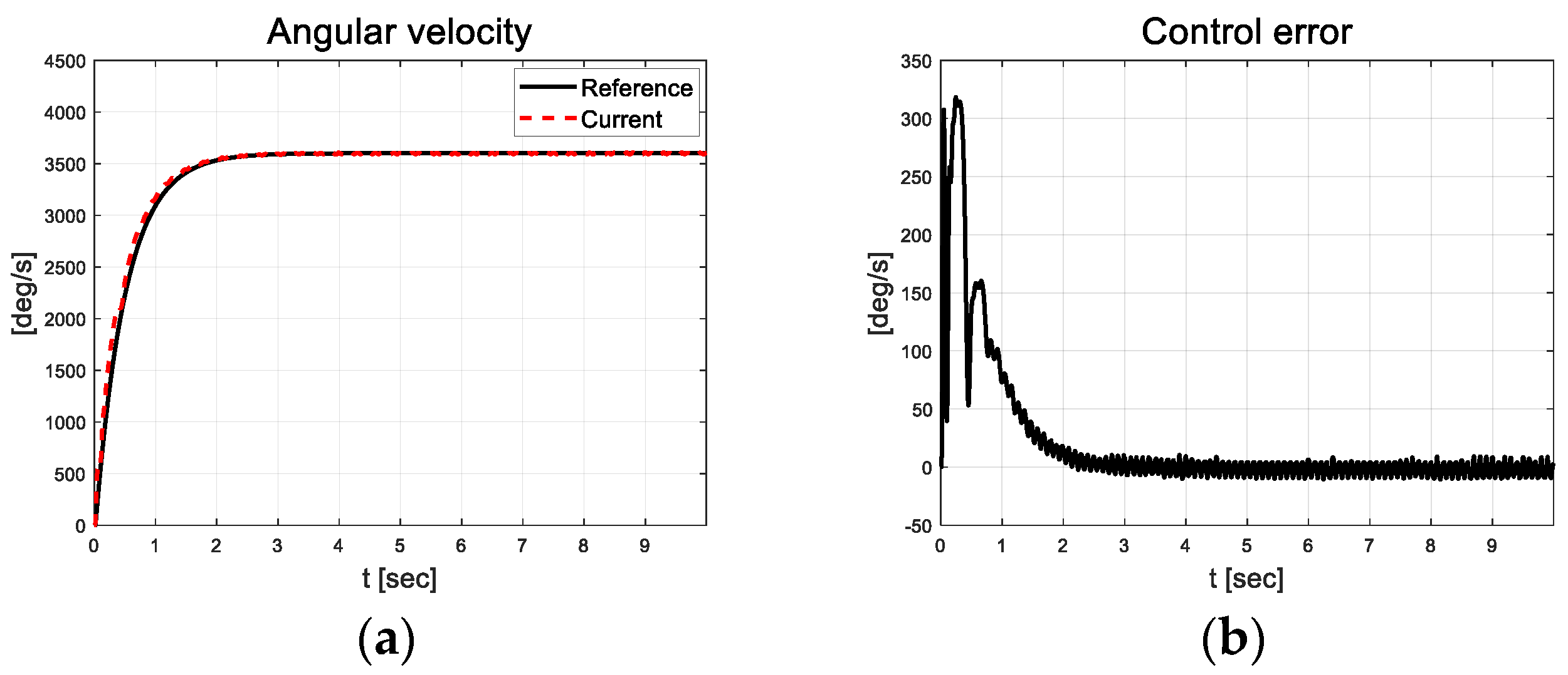
These parameters were determined using a trial-and-error method. In control parameter determination, determining parameters using the trial-and-error technique is relatively time consuming due to multiple failed attempts. Ref. [32] proposed an adaptive neuro-fuzzy inference methodology to determine parameters that improve the stability of the system without careful tuning to achieve optimal performance. In the future, we aim to advance the parameter determination method and plan to prove the robustness of the control algorithm by comparing and analyzing various determined parameter sets for evaluation scenarios, as in [33]. As depicted in Figure 2, the inertia of the rotating disk is relatively small and friction is low; therefore, micro-tuning of the control parameters is considered necessary for velocity tracking. Figure 3 depicts the angular velocity and control error results of the DC motor.

Figure 3.
Velocity tracking result: (a) Velocity; (b) Error.
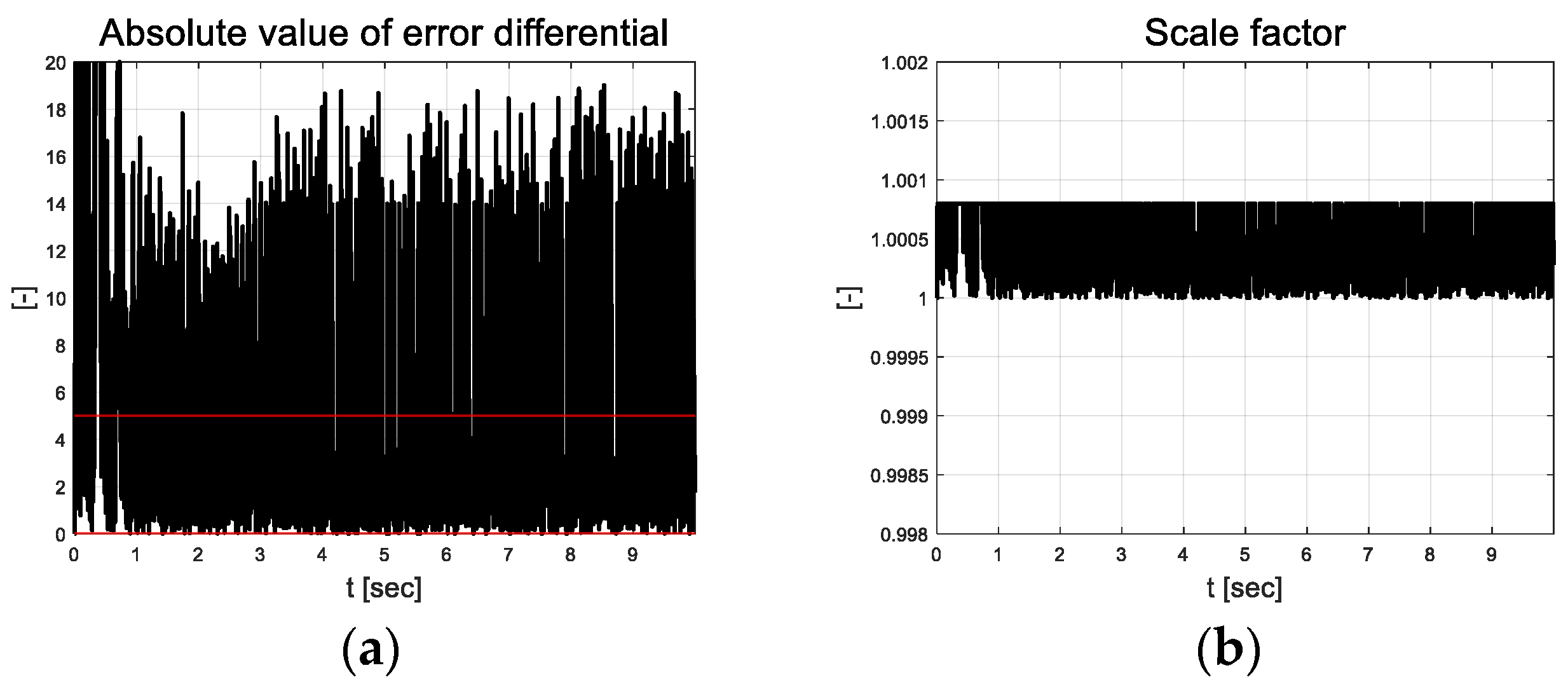
From the angular velocity tracking results depicted in Figure 3, it is evident that the errors were approximately 318 deg/s in the initial transition section. After 2 s, the error decreased to a value closer to zero but chattering occurred (RMS value of 5.34 deg/s). To ensure initial convergence performance, a high-grade sigmoid function or initial value of RLS can be applied; however, this may lead to unreasonable results as chattering that occurs in the actual platform also increases. Figure 4 depicts the scale factor results calculated as the absolute of the error using the threshold values(red line) listed in Table 2.
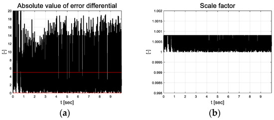
Figure 4.
Path tracking result: (a) Absolute value of error differential; (b) Scale factor.
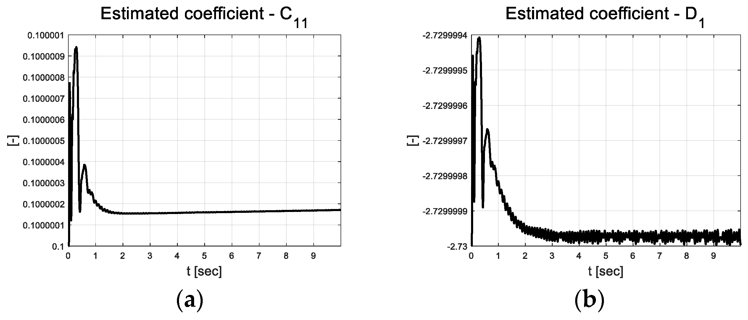
The error graph indicates the chattering phenomenon. In Figure 4, this is illustrated in more detail by indicating the rate of change of the chattering error. This is because the scale factor applied to the covariance update of RLS uses it. The scale factor also resulted in chattering between the upper and lower limits. This results in more sensitive estimates compared to that of RLS, which applies an existing covariance of one. Figure 5a depicts the error dynamics coefficients that are estimated based on RLS using forgetting factors. Although this is an extremely small value, the coefficients apparently change. Constant , which is multiplied by the error, has a significant impact on the control input depending on the error; therefore, it was estimated as a value smaller than .

Figure 5.
Velocity tracking result: (a) Estimated coefficient ; (b) Estimated coefficient .
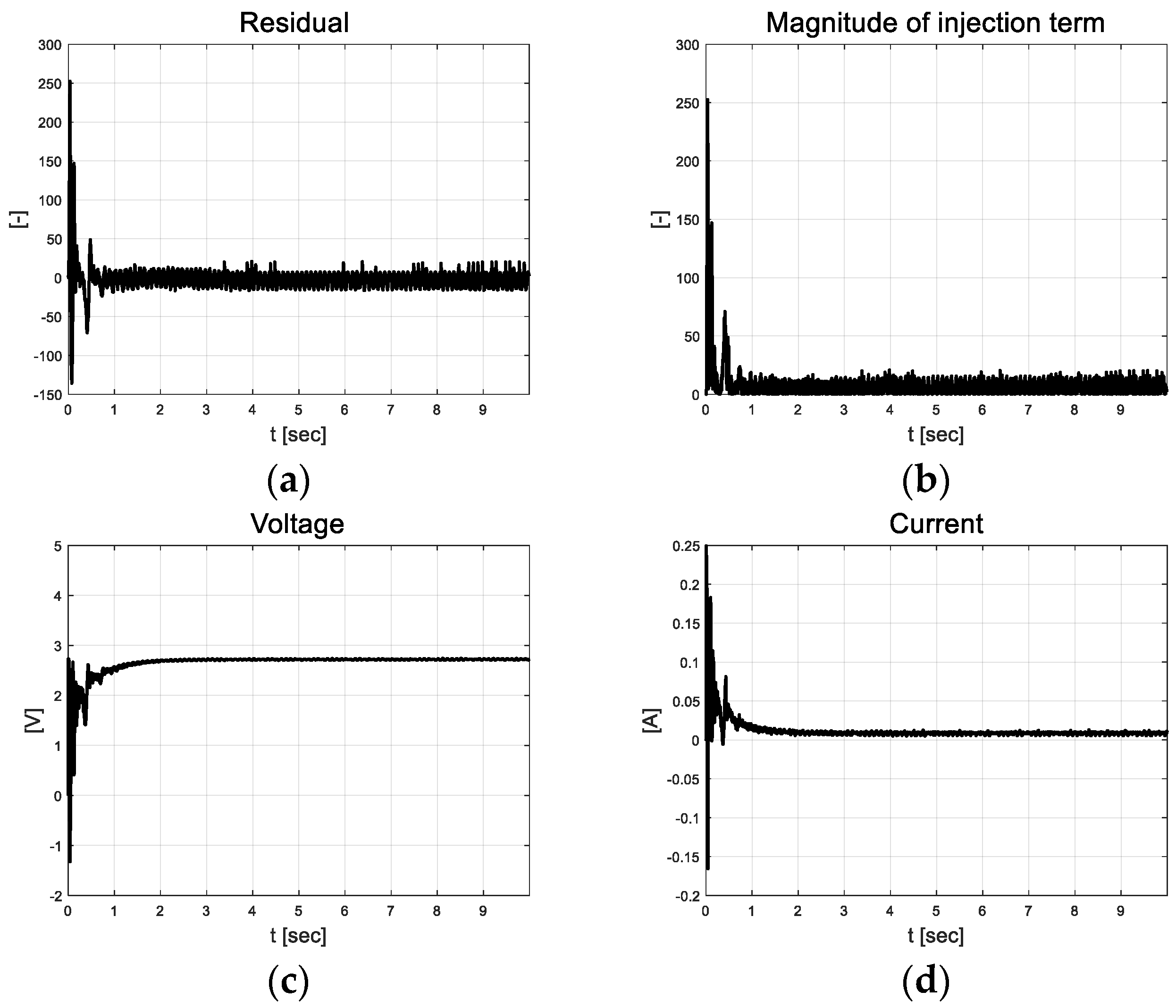
The coefficient estimation residual is depicted in Figure 6a, and the magnitude of the injection term that was calculated using the absolute value of the residual is depicted in Figure 6b. The control inputs using self-tuned injection terms and estimation coefficients, and currents, are depicted in Figure 6c and Figure 6d, respectively.

Figure 6.
Velocity tracking result: (a) Residual; (b) Magnitude of injection term; (c) Voltage; (d) Current.
In the case of a DC motor system, as previously mentioned, the inertia for control and friction is significantly small. Therefore, they react sensitively to small control inputs and exhibit chattering. To control the sensitive system in a more stable manner, a relatively small covariance and estimated initial values were applied. The forgetting factor was set in close proximity to one to remember plenty of previous data, and the scale factor updates the covariance so that the resulting system does not become insensitive.
3.2. Performance Evaluation of CarMaker-Based Adaptive Path Tracking Control
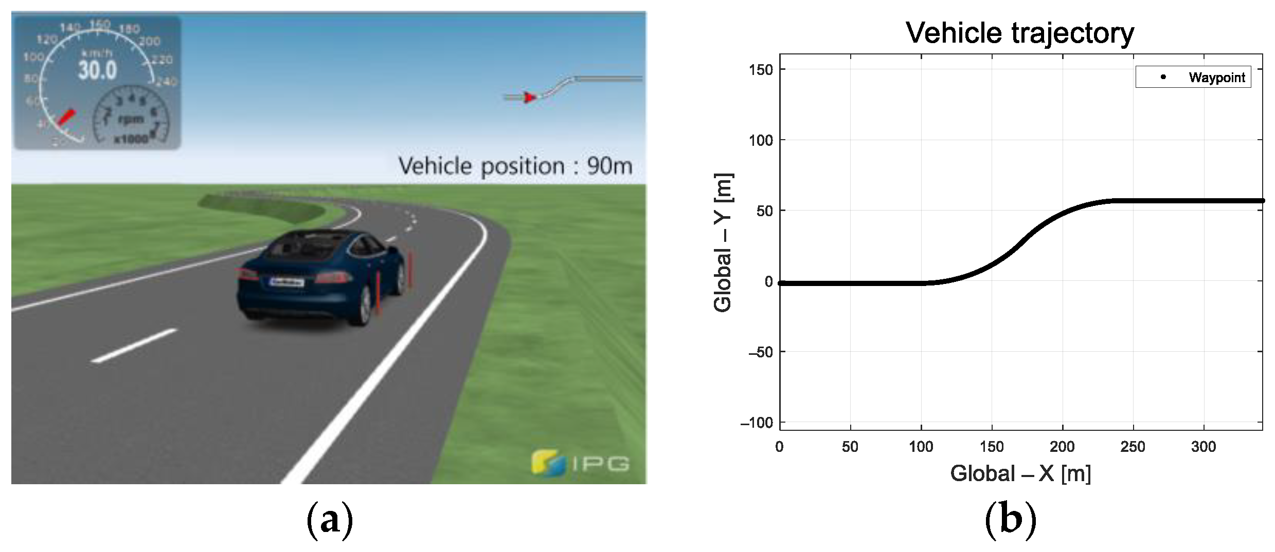
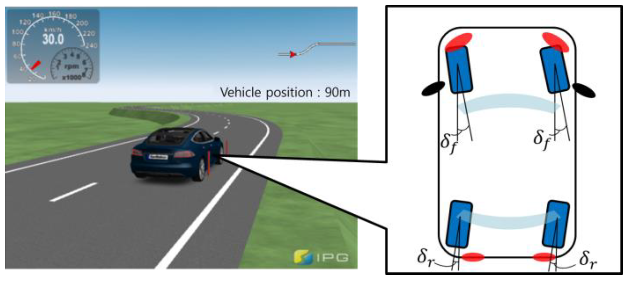
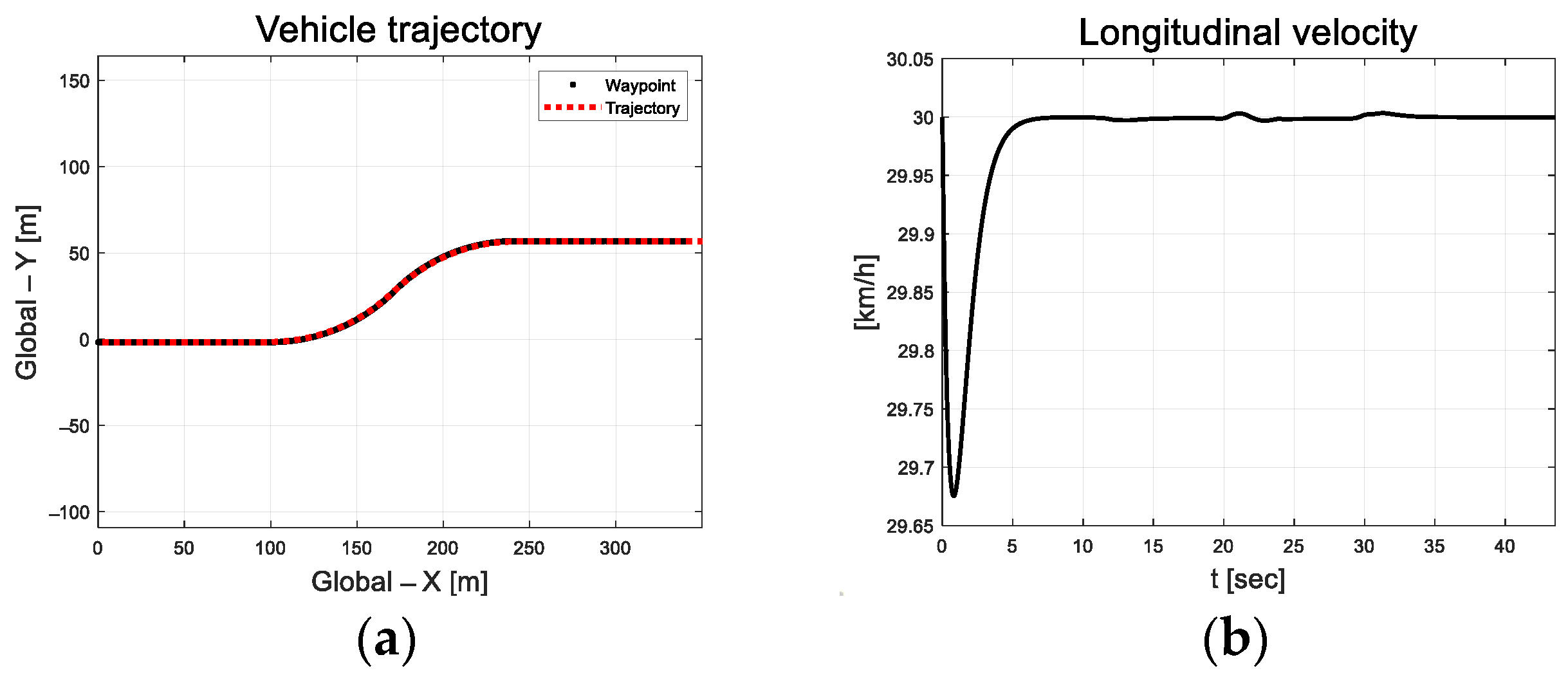
The performance of the proposed algorithm was evaluated using an IPG/CarMaker-based simulation. The trajectory of the target S-curved road is depicted in Figure 7. Table 3 lists the vehicle parameters used for the simulation-based performance evaluation. The velocity was set to 30 kmph and the CarMaker driver model was used for the pedal control.

Figure 7.
Evaluation environment: (a) Vehicle used in IPG/CarMaker; (b) Vehicle trajectory.

Table 3.
Vehicle parameters for proposed controller.
3.2.1. Front-Wheel Steering Vehicle-Based Adaptive Path Tracking Control
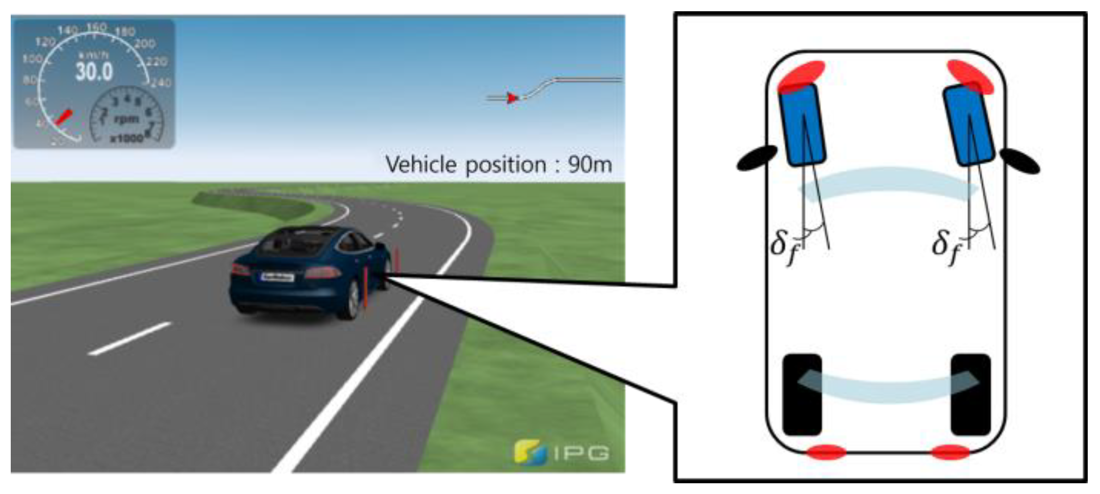
As depicted in Figure 8, the control input derived for path tracking was applied equally to the front wheels of the CarMaker’s vehicle model to evaluate the versatility of the proposed algorithm for front-wheel steering vehicles.
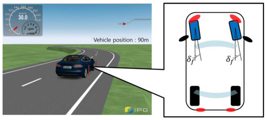
Figure 8.
Concept diagram of front-wheel steering vehicle configuration.
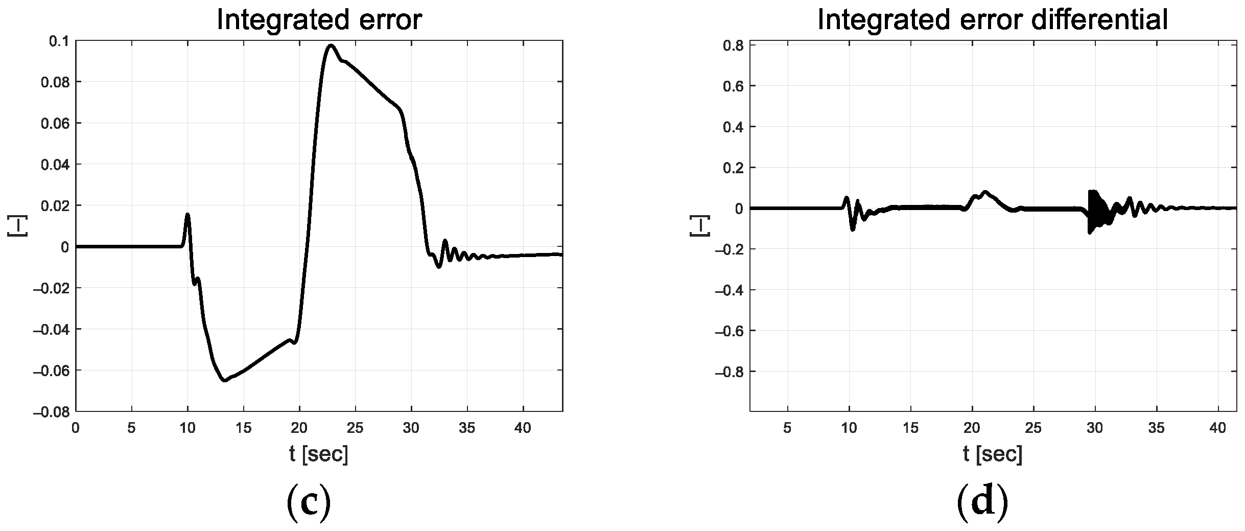
The integrated error () was designed using the lateral preview error and yaw angle error, as shown in Equation (25). The error dynamics are defined in Equation (26). The design variables of the adaptive steering control algorithm are listed in Table 4.

Table 4.
Design parameters of front-wheel steering vehicle adaptive steering control.
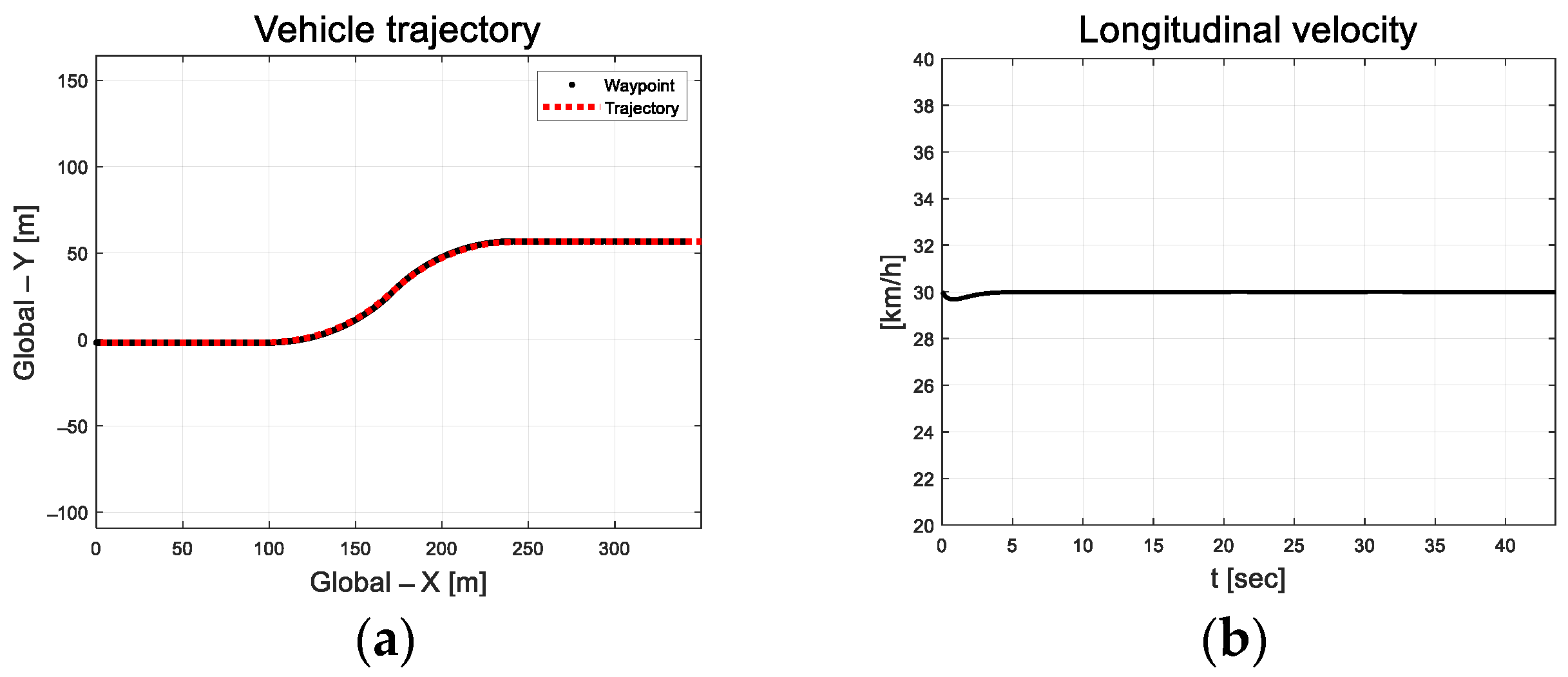
Compared to the previous DC motor platform, the vehicle had a large system inertia; therefore, the design parameters were set to relatively large values. The designed path is an S-curve that includes straight and curved roads, as depicted in Figure 9.
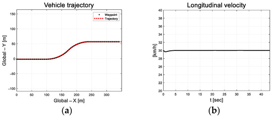
Figure 9.
Path tracking result: (a) Trajectory; (b) Longitudinal velocity.
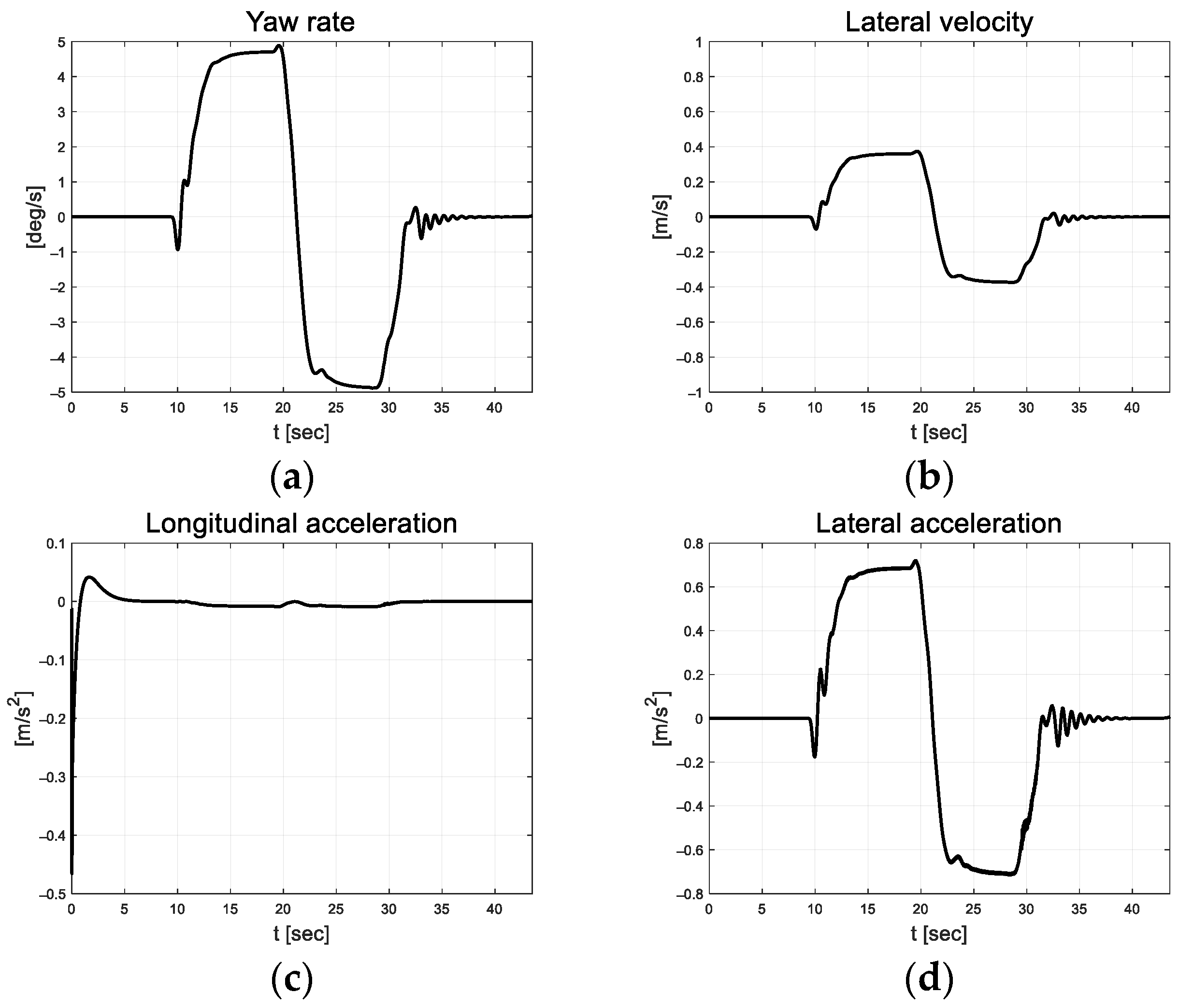
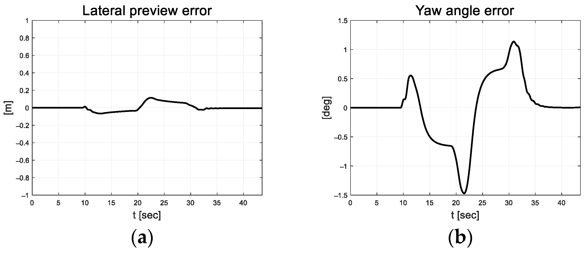
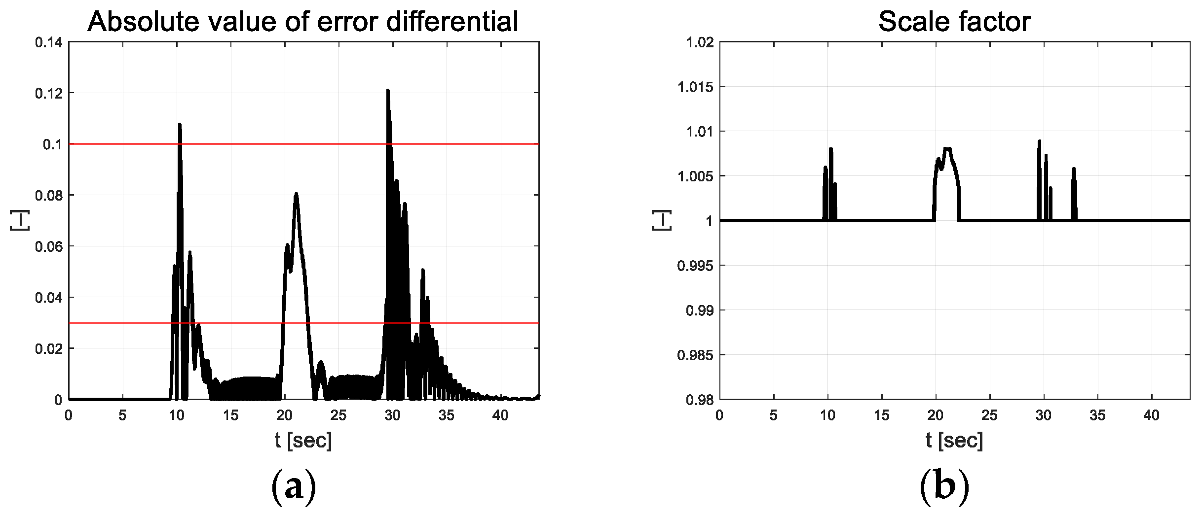
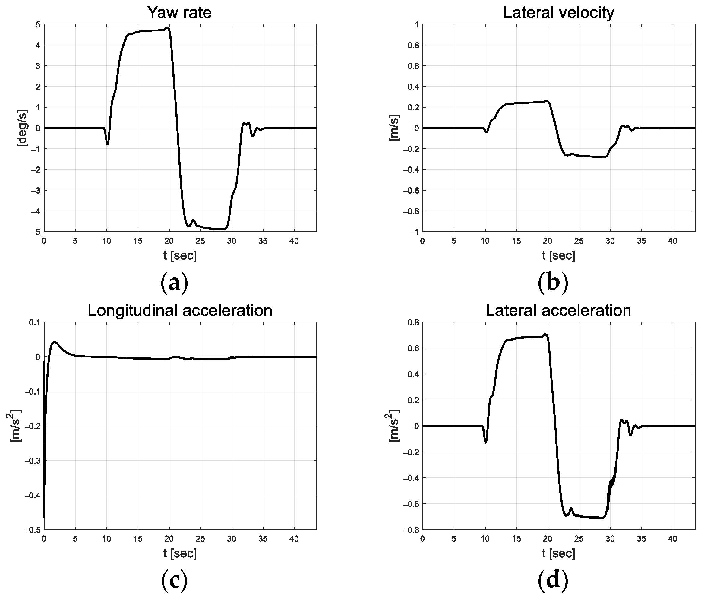
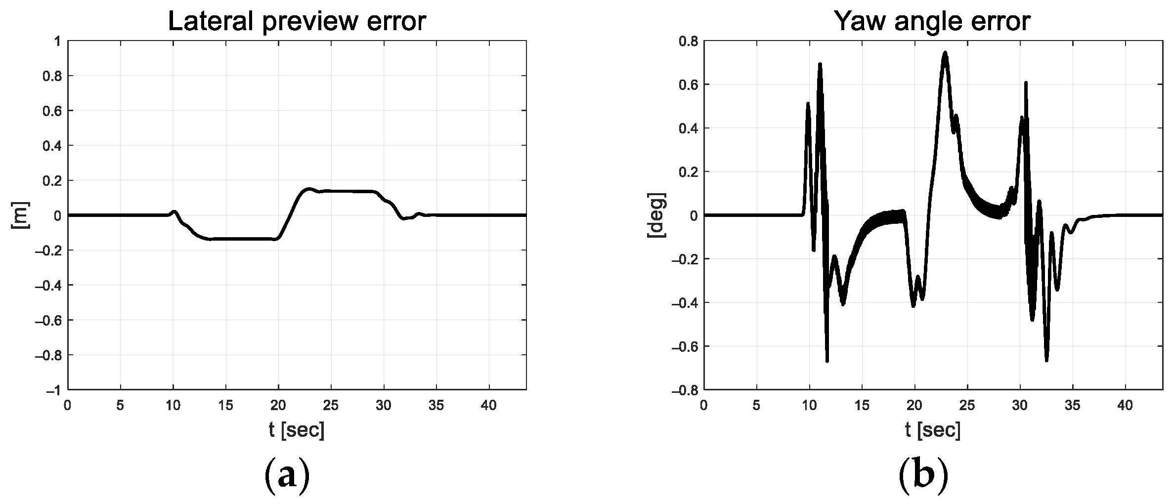
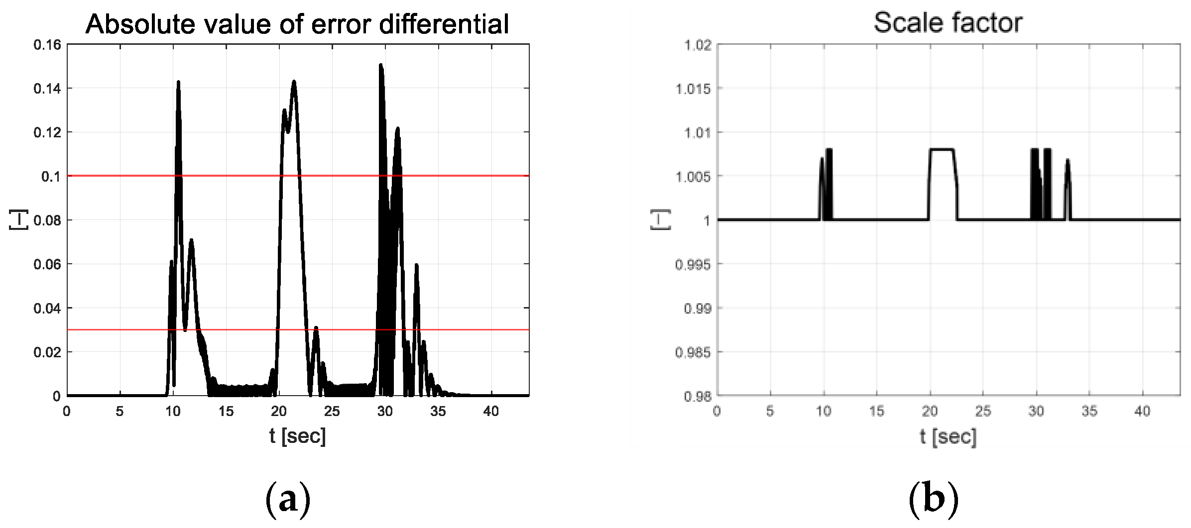
In Figure 10, the vehicle oscillation is visible for approximately 5 s in the section where a straight road and a curved road change; however, the magnitude is small. At approximately 33 s, the robot appears to react to the changing road surface in real time and gradually finds stability as it adapts. Figure 11 depicts the lateral preview and yaw angle errors. From the lateral preview errors, it is evident that symmetry appears for the curved paths. The scale-factor calculated using the absolute values of the error differential is depicted in Figure 12. The scale factor is calculated in real time with the absolute value of the error within the threshold range of 0.03 and 0.1 (red lines in Figure 12).
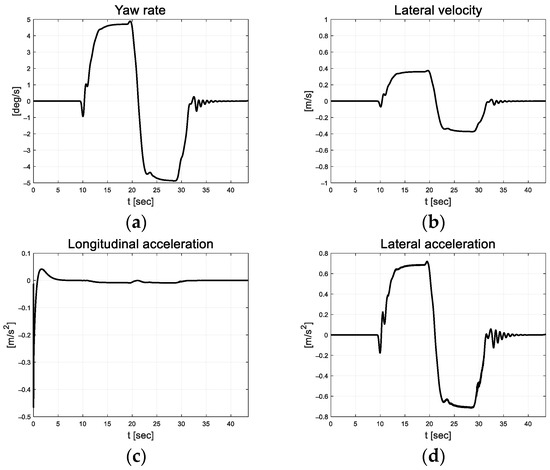
Figure 10.
Path tracking result: (a) Yaw rate; (b) Lateral velocity; (c) Longitudinal acceleration; (d) Lateral acceleration.


Figure 11.
Path tracking result: (a) Lateral preview error; (b) Yaw angle error; (c) Integrated error; (d) Integrated error differential.

Figure 12.
Path tracking result: (a) Absolute value of error differential; (b) Scale factor.
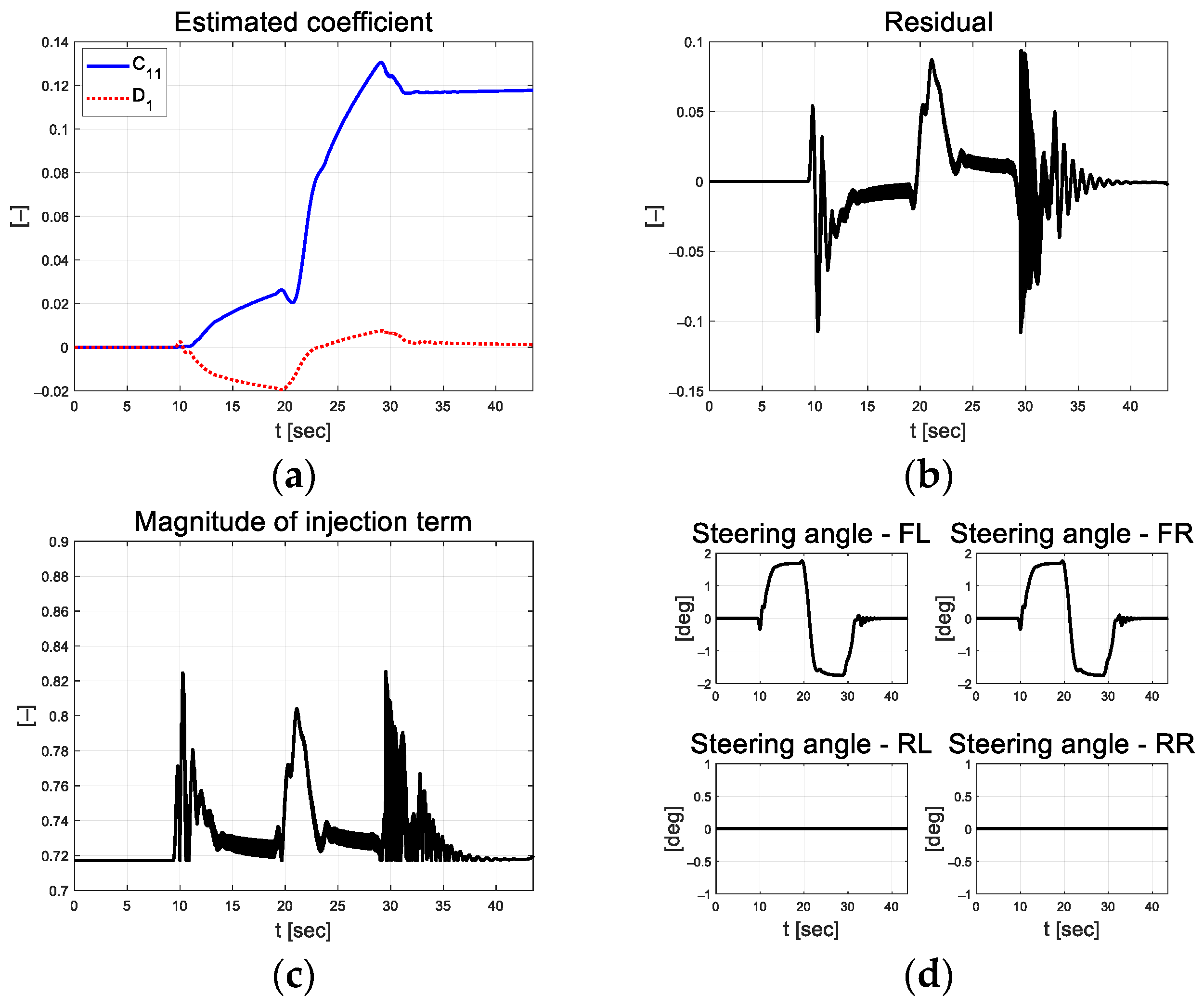
Based on the threshold set listed in Table 4, the scale factor of the value smaller than the lower limit of 0.03 is 1 and larger than the upper limit of 0.1 is 1.008. Figure 13a depicts the coefficients estimated using RLS. The RLS estimation coefficient is updated in curved driving and exhibits convergence results in straight driving. Figure 13b depicts the residual at this time. This indicates that residuals occur during curved driving. The magnitudes of the injection terms are depicted in Figure 13c,d as control inputs.

Figure 13.
Path tracking result: (a) Estimated coefficient; (b) Residual; (c) Injection; (d) Control input.
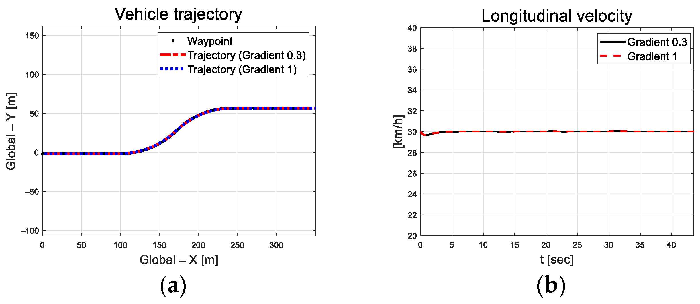
As mentioned in Equation (22), in the above performance evaluation, the sigmoid function was applied to the injection term for chattering attenuation. In this study, the chattering phenomenon of control input was analyzed using two gradient values of the sigmoid function used for the injection term, and the evaluation results are as follows. Figure 14 shows the derived trajectory and longitudinal velocity results of tracking performance by applying the two gradient values (0.3 and 1) of the sigmoid function for the injection term.
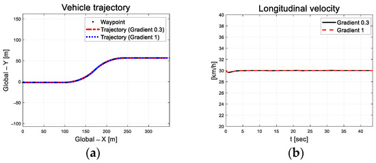
Figure 14.
Path tracking result: (a) Trajectory; (b) Longitudinal velocity.
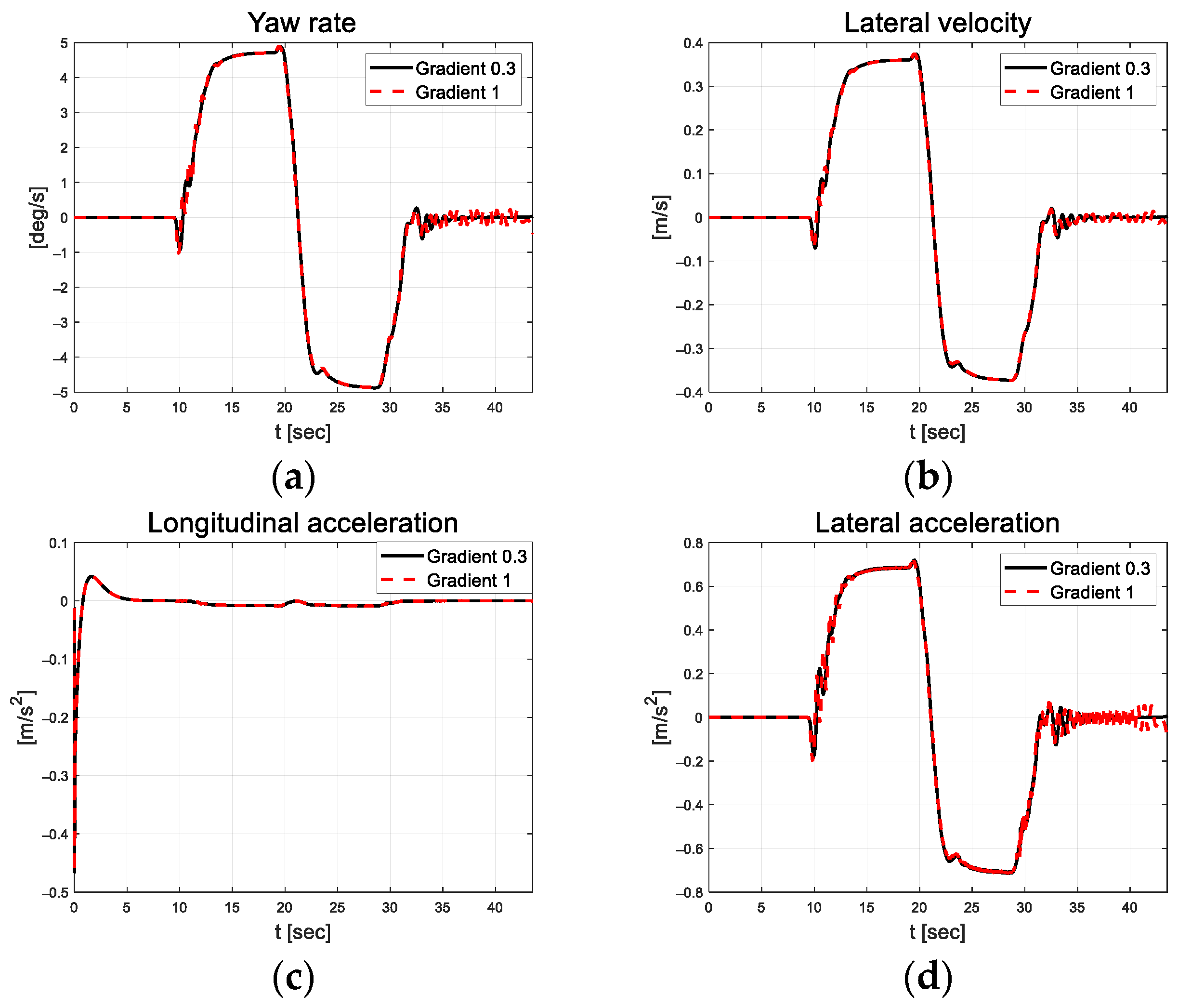
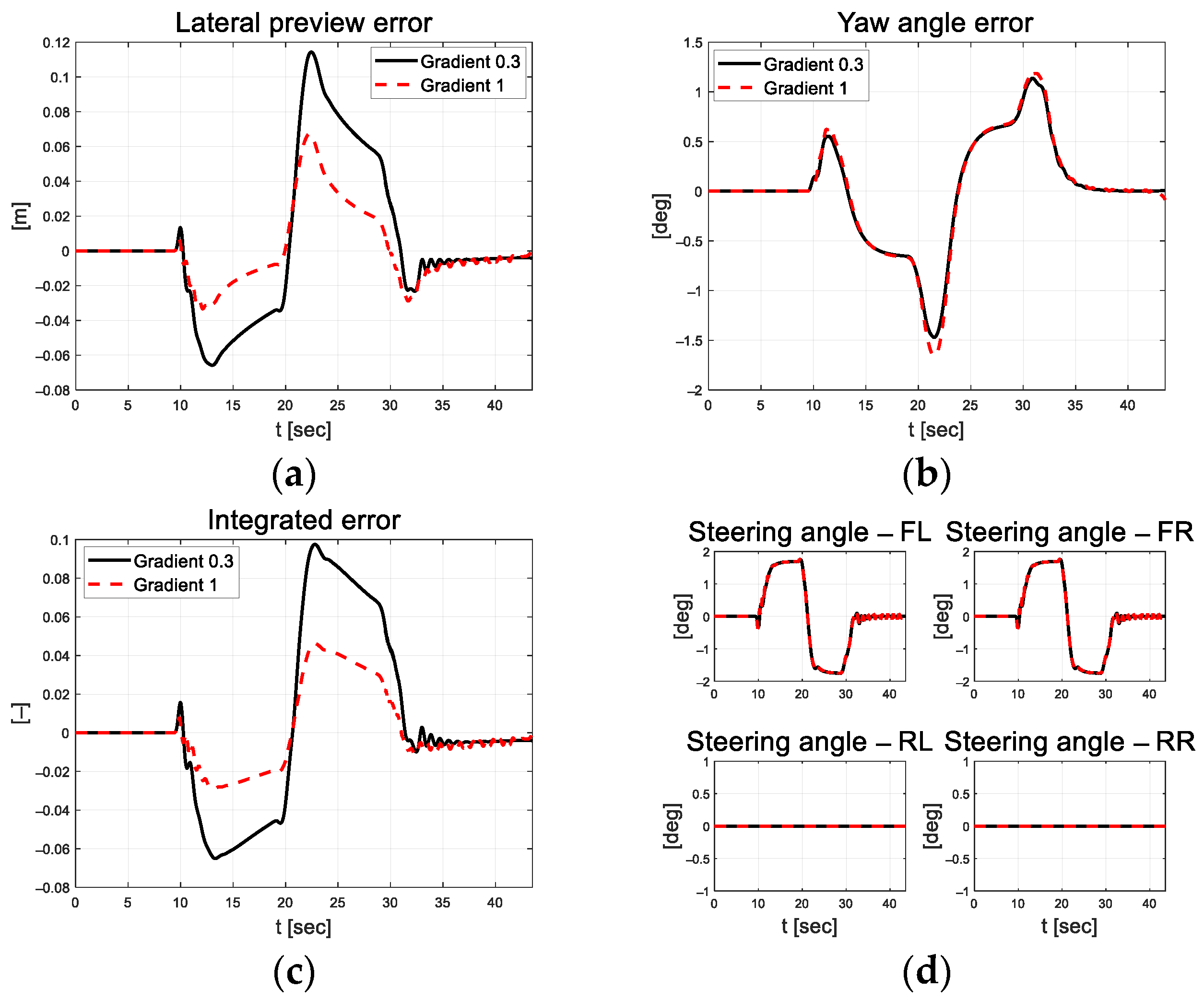
In Figure 15, there is no significant difference in the longitudinal velocity, but as the slope of the sigmoid function increases, it is observed that the oscillation of yaw rate, lateral velocity, and lateral acceleration also increases generally. In particular, on the straight road after the curved road, it can be seen that relatively large oscillations occur in both the negative and positive directions, with the error centered at 0. In Figure 16, the magnitude of the integrated error was reduced, but it is difficult to analyze the control stability only using control error due to the oscillation of the steering angle.
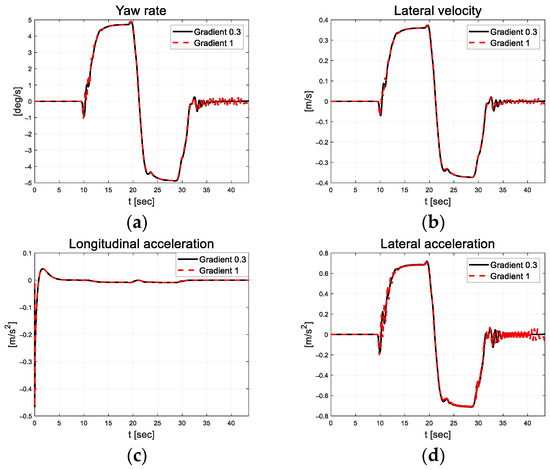
Figure 15.
Path tracking result: (a) Yaw rate; (b) Lateral velocity; (c) Longitudinal acceleration; (d) Lateral acceleration.
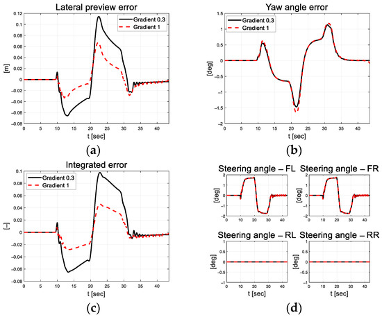
Figure 16.
Path tracking result: (a) Lateral preview error; (b) Yaw angle error; (c) Integrated error; (d) Control input.
Through analysis of the above provided results, it was confirmed that an increase in the gradient of the sigmoid function can cause an increase of the chattering phenomenon. Based on the results analysis, it was found that the using the sigmoid function can play a role for chattering attenuation.
3.2.2. Front-and-Rear-Wheel Steering Vehicle-Based Adaptive Path Tracking Control
As depicted in Figure 17, the front-and-rear-wheel control inputs derived for path tracking were applied equally to the left and right wheels, respectively. Because the vehicle is driven at a relatively low speed, the front-and-rear-wheel steering inputs are derived in opposite phases.
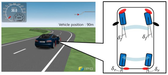
Figure 17.
Concept diagram of front-and-rear-wheel steering vehicle configuration.
In this section, the error dynamics of the front and rear wheels are designed using the lateral preview error and yaw angle error, respectively, as expressed in Equation (27). The control input for was defined as the front-wheel steering angle and the control input for was defined as the rear-wheel steering angle , and the adaptive steering control input based on Equation (23) was derived as shown in Equation (28).
As listed in Table 5, the same values were applied to the decay rate of the Lyapunov function and reachability factor to derive the front-and-rear-wheel steering angles.

Table 5.
Design parameters for front-wheel steering vehicle adaptive steering control.
The parameters were determined using a trial-and-error method. Compared to the previously mentioned DC motor platform, the vehicle has a large system inertia; therefore, the forgetting factor and initial value were set to relatively large values. Figure 18 depicts the results of driving along the target path without lane departure.
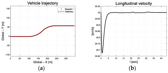
Figure 18.
Path tracking result: (a) Trajectory; (b) Longitudinal velocity.
In Figure 19, the results of the front-and-rear-wheel steering cases indicate that the lateral velocity is lower than that of the front-wheel steering case. Figure 20 depicts the lateral preview and yaw angle errors of the target path. However, active steering occurs because of the rear-wheel steering intervention, and the sign of the lateral preview error is reversed compared to the front-wheel steering case.

Figure 19.
Path tracking result: (a) Yaw rate; (b) Lateral velocity; (c) Longitudinal acceleration; (d) Lateral acceleration.

Figure 20.
Path tracking result: (a) Lateral preview error; (b) Yaw angle error.
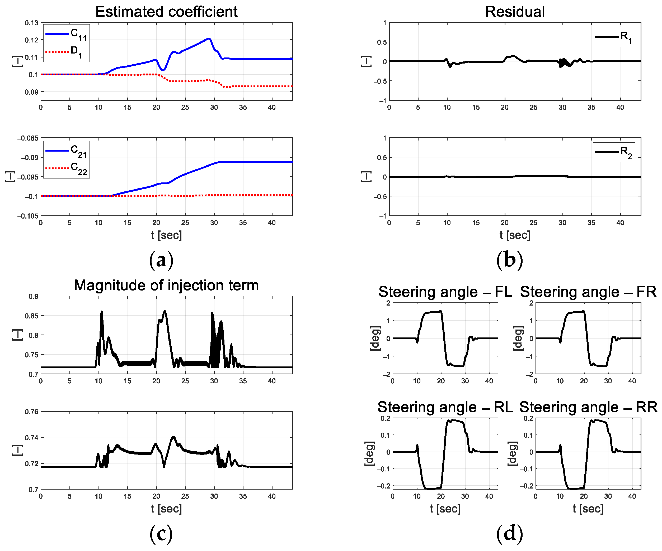
Figure 21 depicts the scale-factor results calculated over a threshold range (red line) set using the absolute value of the error difference. This assists in updating the covariance so that estimates can respond and converge quickly in curved driving sections. Figure 22a depicts the coefficients estimated using RLS in real time. The estimated coefficients for the rear wheels were smaller than those for the front wheels. Figure 22b depicts the residual estimated at this time. The magnitude of the injection term calculated using the residual is depicted in Figure 22c, and the control input result calculated using this is depicted in Figure 22d. This shows that the rear-wheel steering angle is in the opposite phase and is small compared to the front-wheel steering angle.
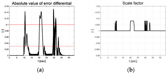
Figure 21.
Path tracking result: (a) Absolute value of error differential; (b) Scale factor.
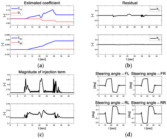
Figure 22.
Path tracking result: (a) Estimated coefficient; (b) Residual; (c) Injection; (d) Control input.
Proof.
First, the cost function designed is as follows:
For stable control, the derivative of the cost function with respect to time must be negative. By differentiation of the cost function with respect to time and substitution of the control input term with the designed control input, the following equations can be derived.
Here, the difference between the estimated and the measured value is converted into a residual, and the magnitude of the defined injection term is substituted.
From the derived cost function, control stability is analyzed according to the signs of the residuals and errors (five cases).
It has been proven that the cost function is less than or equal to zero in all possible residual and error signs. □
4. Discussion
The performance of the proposed universal-purpose adaptive control algorithm for the MIMO system was evaluated using a DC motor, front-wheel steering vehicle, and front-and-rear-wheel steering vehicle. These scenarios were set to simulate an environment that can improve work efficiency and engineer convenience through universal applications on various platforms with the advancement in technology. No information from the system is required for target-value tracking. For RLS-based coefficient estimation, only a few control parameters, such as initial values and forgetting factors, are required. The evaluation results confirm that a reasonable target-value tracking performance of the adaptive control input is finally derived through the RLS-based real-time estimated coefficients. The DC motor system has a significantly small inertia and friction to control; therefore, it reacts sensitively to the control input and chattering occurs. As such, the RLS-based coefficient estimation is sensitive to the initial parameter settings. This was performed using a trial-and-error method and a micro-tuning methodology. Furthermore, an oscillation phenomenon was confirmed in the straight driving section during the last curved drive. The oscillation worsened in the rear-wheel steering scenarios. Oscillation, which is revealed as a vehicle condition quantity, has a relatively small value; however, it can affect target-value tracking when driving at high speeds. The goal is to solve this problem through a more stable control in the future, and an evaluation of the actual mobility.
5. Conclusions
In this study, we proposed a universal-purpose adaptive control algorithm using a sliding-mode approach and parameter self-tuning. We defined several error dynamics based on the control errors. The control error of each system can be integrated and controlled by applying weights. To design a sliding-mode approach without system information, we estimated the coefficients for the RLS-based error dynamics. The control error and estimation coefficients were then used to derive the magnitude of the injection term and adaptive control input. The purpose of this study was to easily apply the same controller to various platforms and achieve target-value tracking performance with the advancement in technology. Adaptive control input derivation does not require any information from the system. This is achieved by estimating the coefficients of the error dynamics using RLS in real time. In addition, by applying a self-tuning injection term according to the magnitude of the control error, the control error can be quickly reduced to zero while complying with the finite-time convergence condition. The evaluation was conducted using actual DC motor platforms, CarMaker-based front-wheel steering vehicles, and front-and-rear-wheel steering vehicles. The evaluation results demonstrated that the proposed control algorithm tracks the target value reasonably without any information from the system. This is expected to improve the engineers’ efficiency and convenience by universally applying the same controller to various systems. However, chattering was observed in the control input and system states. Chattering affected the residuals used in control input calculations, and thus led to chattering of the control inputs. Our goal was to develop algorithms that minimize chattering by deriving stable control inputs. In addition, our goal was to advance the control algorithm by applying an integral term to rapidly converge to relatively large errors during the initial stage. Moreover, we intend to expand the application of the universal controller to environmental configurations, such as high-speed driving and evaluation using actual mobility platforms.
Author Contributions
Conceptualization, K.O.; methodology, H.L. and K.O.; software, H.L.; validation, H.L.; formal analysis, H.L. and K.O.; investigation, H.L.; resources, H.L.; data curation, H.L.; writing—original draft preparation, H.L.; writing—review and editing, H.L. and K.O.; visualization, H.L.; supervision, K.O.; project administration, K.O.; funding acquisition, K.O. All authors have read and agreed to the published version of the manuscript.
Funding
This research was funded by the National Research Foundation of Korea (NRF-2022R1F1A1075167) and government funding (Ministry of Science and ICT) in 2022.
Data Availability Statement
Data sharing is not applicable to this article.
Conflicts of Interest
The authors declare no conflict of interest.
References
- Liu, K.; Meng, F.; Meng, S.; Wang, C. Robust Controller Design for Multi-Input Multi-Output systems using coefficient diagram method. Entropy 2021, 23, 1180. [Google Scholar] [CrossRef] [PubMed]
- Homaeinezhad, M.R.; Mostaghim, M.S. Synthetic Lyapunov stabilization technique for designing actuation-constrained multi-input multi-output control systems. J. Franklin. Inst. 2022, 359, 5891–5918. [Google Scholar] [CrossRef]
- Pongfai, J.; Angeli, C.; Shi, P.; Su, X.; Assawinchaichote, W. Optimal PID controller autotuning design for MIMO nonlinear systems based on the adaptive SLP algorithm. Int. J. Control Autom. Syst. 2021, 19, 392–403. [Google Scholar] [CrossRef]
- Homaeinezhad, M.R.; Ebrahimi, M.M. Tracking control stabilization of systems manipulated by constrained parabolic nonlinear actuator. Int. J. Dyn. Control 2023, 1–18. [Google Scholar] [CrossRef]
- Dhananjaya, M.; Ponuru, D.; Babu, T.S.; Aljafari, B.; Alhelou, H.H. A new multi-output DC-DC converter for electric vehicle application. IEEE Access 2022, 10, 19072–19082. [Google Scholar] [CrossRef]
- Al-Mahturi, A.; Santoso, F.; Garratt, M.A.; Anavatti, S.G. A Robust Self-Adaptive Interval Type-2 TS Fuzzy Logic for Controlling Multi-Input–Multi-Output Nonlinear Uncertain Dynamical Systems. IEEE Trans. Syst. Man Cybern. Syst. 2020, 52, 655–666. [Google Scholar] [CrossRef]
- Mecifi, M.; Boumediene, A.; Boubekeur, D. Fuzzy sliding mode control for trajectory tracking of an electric powered wheelchair. AIMS Electron. Electr. Eng. 2021, 5, 176–193. [Google Scholar] [CrossRef]
- Huang, X.; Song, Y. Distributed and performance guaranteed robust control for uncertain MIMO nonlinear systems with controllability relaxation. IEEE Trans. Autom. Control 2022, 68, 2460–2467. [Google Scholar] [CrossRef]
- Thanh, H.L.N.N.; Vu, M.T.; Nguyen, N.P.; Mung, N.X.; Hong, S.K. Finite-time stability of MIMO nonlinear systems based on robust adaptive sliding control: Methodology and application to stabilize chaotic motions. IEEE Access 2021, 9, 21759–21768. [Google Scholar] [CrossRef]
- Zeghlache, S.; Benyettou, L.; Djerioui, A.; Ghellab, M.Z. Twin rotor MIMO system experimental validation of robust adaptive fuzzy control against wind effects. IEEE Syst. J. 2020, 16, 409–419. [Google Scholar] [CrossRef]
- Usman, H.M.; Mukhopadhyay, S.; Rehman, H. Permanent magnet DC motor parameters estimation via universal adaptive stabilization. Control Eng. Pract. 2019, 90, 50–62. [Google Scholar] [CrossRef]
- Laid, S.; Boubekeur, B. Model-free and adaptive control of a dc motor: A comparative study. In Proceedings of the 2020 International Conference on Electrical Engineering, Istanbul, Turkey, 25–27 September 2020; pp. 1–6. [Google Scholar]
- Mynar, Z.; Vaclavek, P.; Blaha, P. Synchronous reluctance motor parameter and state estimation using extended Kalman filter and current derivative measurement. IEEE Trans. Ind. Electron. 2020, 68, 1972–1981. [Google Scholar] [CrossRef]
- Jiang, Y.; Xu, X.; Zhang, L. Heading tracking of 6WID/4WIS unmanned ground vehicles with variable wheelbase based on model free adaptive control. Mech. Syst. Signal Process. 2021, 159, 107715. [Google Scholar] [CrossRef]
- Wang, J.; Tan, G.; Sun, C. Research on vehicle four-wheel steering based on model-free adaptive control. In Proceedings of the 2020 5th International Conference on Electromechanical Control Technology and Transportation, Nanchang, China, 15–17 May 2020; pp. 372–376. [Google Scholar]
- Fliess, M.; Join, C. An alternative to proportional-integral and proportional-integral-derivative regulators: Intelligent proportional-derivative regulators. Int. J. Robust Nonlinear Control 2022, 32, 9512–9524. [Google Scholar] [CrossRef]
- Liu, S.; Hou, Z.; Tian, T.; Deng, Z.; Li, Z. A novel dual successive projection-based model-free adaptive control method and application to an autonomous car. IEEE Trans. Neural Netw. Learn. Syst. 2019, 30, 3444–3457. [Google Scholar] [CrossRef] [PubMed]
- Moreno-Gonzalez, M.; Artuñedo, A.; Villagra, J.; Join, C.; Fliess, M. Speed-adaptive model-free lateral control for automated cars. IFAC-PapersOnLine 2022, 55, 84–89. [Google Scholar] [CrossRef]
- Farhan, A.; Abdelrahem, M.; Saleh, A.; Shaltout, A.; Kennel, R. Simplified sensorless current predictive control of synchronous reluctance motor using online parameter estimation. Energies 2020, 13, 492. [Google Scholar] [CrossRef]
- Wang, Z.; Wang, J. Ultra-local model predictive control: A model-free approach and its application on automated vehicle trajectory tracking. Control Eng. Pract. 2020, 101, 104482. [Google Scholar] [CrossRef]
- Zhang, X.; Zhu, X. Autonomous path tracking control of intelligent electric vehicles based on lane detection and optimal preview method. Expert Syst. Appl. 2019, 121, 38–48. [Google Scholar] [CrossRef]
- Matraji, I.; Al-Wahedi, K.; Al-Durra, A. Higher-order super-twisting control for trajectory tracking control of skid-steered mobile robot. IEEE Access 2020, 8, 124712–124721. [Google Scholar] [CrossRef]
- Moudoud, B.; Aissaoui, H.; Diany, M. Robust trajectory tracking control based on sliding mode of Differential Driving FourWheeled Mobile Robot. In Proceedings of the 2020 IEEE 6th International Conference on Optimization and Applications, Beni Mellal, Morocco, 20–21 April 2020; pp. 1–5. [Google Scholar]
- Fnadi, M.; Plumet, F.; Benamar, F. Model predictive control based dynamic path tracking of a four-wheel steering mobile robot. In Proceedings of the 2019 IEEE/RSJ International Conference on Intelligent Robots and Systems, Macau, China, 3–8 November 2019; pp. 4518–4523. [Google Scholar]
- Bai, G.; Liu, L.; Meng, Y.; Luo, W.; Gu, Q.; Wang, J. Path tracking of wheeled mobile robots based on dynamic prediction model. IEEE Access 2019, 7, 39690–39701. [Google Scholar] [CrossRef]
- Mohammadzadeh, A.; Taghavifar, H. A novel adaptive control approach for path tracking control of autonomous vehicles subject to uncertain dynamics. Proc. Inst. Mech. Eng. Part D J. Automob. Eng. 2020, 234, 2115–2126. [Google Scholar] [CrossRef]
- Chen, I.M.; Chan, C.Y. Deep reinforcement learning based path tracking controller for autonomous vehicle. Proc. Inst. Mech. Eng. Part D J. Automob. Eng. 2021, 235, 541–551. [Google Scholar] [CrossRef]
- Shan, Y.; Zheng, B.; Chen, L.; Chen, L.; Chen, D. A reinforcement learning-based adaptive path tracking approach for autonomous driving. IEEE Trans. Veh. Technol. 2020, 69, 10581–10595. [Google Scholar] [CrossRef]
- Moudoud, B.; Aissaoui, H.; Diany, M. Fuzzy adaptive sliding mode controller for electrically driven wheeled mobile robot for trajectory tracking task. J. Control Decis. 2022, 9, 71–79. [Google Scholar] [CrossRef]
- Aware, P.; Hanwate, S.; Wanaskar, V. Yaw rate and sideslip angle control of active 4WS using a two-time scale based novel sliding mode control. In Proceedings of the 2021 5th International Conference on Intelligent Computing and Control Systems, Madurai, India, 6–8 May 2021; pp. 548–553. [Google Scholar]
- Vahidi, A.; Stefanopoulou, A.; Peng, H. Recursive least squares with forgetting for online estimation of vehicle mass and road grade: Theory and experiments. Veh. Syst. Dyn. 2011, 43, 31–55. [Google Scholar] [CrossRef]
- George, J.; Mani, G. A Portrayal of Sliding Mode Control through Adaptive Neuro Fuzzy Inference System with Optimization Perspective. IEEE Access 2024, 12, 3222–3239. [Google Scholar] [CrossRef]
- Herman, P. Numerical test of several controllers for underactuated underwater vehicles. Appl. Sci. 2020, 10, 8292. [Google Scholar] [CrossRef]
Disclaimer/Publisher’s Note: The statements, opinions and data contained in all publications are solely those of the individual author(s) and contributor(s) and not of MDPI and/or the editor(s). MDPI and/or the editor(s) disclaim responsibility for any injury to people or property resulting from any ideas, methods, instructions or products referred to in the content. |
© 2024 by the authors. Licensee MDPI, Basel, Switzerland. This article is an open access article distributed under the terms and conditions of the Creative Commons Attribution (CC BY) license (https://creativecommons.org/licenses/by/4.0/).


