Article

A Novel Extended Unscented Kalman Filter Is Designed Using the Higher-Order Statistical Property of the Approximate Error of the System Model

1
School of Information and Control Engineering, Jilin Institute of Chemical Technology, Jilin 132000, China
2
School of Automation, Guangdong University of Petrochemical Technology, Maoming 525000, China
*
Author to whom correspondence should be addressed.
Actuators 2024, 13(5), 169; https://doi.org/10.3390/act13050169
Submission received: 18 March 2024 / Revised: 22 April 2024 / Accepted: 25 April 2024 / Published: 1 May 2024
(This article belongs to the Special Issue From Theory to Practice: Incremental Nonlinear Control)

Abstract

:
In the actual working environment, most equipment models present nonlinear characteristics. For nonlinear system filtering, filtering methods such as the Extended Kalman Filter (EKF), Unscented Kalman Filter (UKF), and Cubature Kalman Filter (CKF) have been developed successively, all of which show good results. However, in the process of nonlinear system filtering, the performance of EKF decreases with an increase in the truncation error and even diverges. With improvement of the system dimension, the sampling points of UKF are relatively few and unrepresentative. In this paper, a novel high-order extended Unscented Kalman Filter (HUKF) based on an Unscented Kalman Filter is designed using the higher-order statistical properties of the approximate error. In addition, a method for calculating the approximate error of the multi-level approximation of the original function under the condition that the measurement is not rank-satisfied is proposed. The effectiveness of the filter is verified using digital simulation experiments.

1. Introduction

The state estimation is usually implemented by a filter, which uses real-time measurements and dynamic models of the system to improve the data accuracy and obtain the estimated state of the system [1]. In 1960, Kalman proposed a filtering method for linear systems that was soon widely used [2]. It is a time-domain filtering method that describes the target system using a state-space approach and a minimum mean square error (MSE) recursive form [3]. Kalman filtering is a state estimation method that has been widely used in the areas of signal processing, autonomous navigation, and fault diagnosis [2]. KF is optimal for linear filtering and less effective for nonlinear filtering [4]. However, in a practical context, almost all systems are nonlinear [5]. Therefore, with the wide application of Kalman filtering algorithms in engineering practice, Kalman filtering has struggled to meet practical needs. In order to solve the problem of the poor performance of Kalman filtering in dealing with nonlinear systems, the extended Kalman filter (EKF) was proposed by combining Kalman filtering and the Taylor expansion method [6]. It effectively solves the problem of divergence of the Kalman filtering algorithm in nonlinear Gaussian systems. However, because the extended Kalman filtering algorithm only takes the first-order Jacobi matrix and ignores the higher-order terms in the Taylor expansion in the process of converting a nonlinear system to a linear system [7], a truncation error is introduced, and the accumulation of errors in the error covariance matrix during the linearization process also inevitably leads to a loss of filtering accuracy [8]. For strongly nonlinear systems, the Jacobi matrix is not a suitable approximation and may cause the EKF estimation to deviate from the true state trajectory, leading to poor estimation and numerical instability [9]. In order to solve the problem that the truncation error of the extended Kalman filter affects the filtering accuracy, Fredrik Gustafsson et al. [10] proposed the use of a second-order compensation EKF to approximate the residual term and improve the filtering accuracy by compensating the mean and variance of the estimated term. O. A. Stepanov et al. [11] proposed a polynomial filter to improve the estimation accuracy in the case of quadratic nonlinearity and reduce the impact of the error caused by the linearization process. Although these methods improve the estimation accuracy, they require extensive calculation and increase the computational burden owing to the improvement of the order of truncation error. To solve the problems associated with the extended Kalman filter, in 1995, Julier proposed the Unscented Kalman filter (UKF) [12]. The main difference between the EKF and UKF is the model linearization method [13]. The core of the UKF algorithm is the UT transform [14], which is used to linearize a nonlinear function by nonlinearly influencing the sampling points [15]. The UKF can approximate the statistical mean and covariance of any nonlinearity up to the third order [9], although both the EKF and UKF can approximate nonlinear models up to the second order [15]. The UKF is becoming promising, as it performs better in terms of convergence rate and estimation accuracy compared with the EKF [16]. The strength of the UKF lies in the accuracy and efficiency of computation [17]. It is highly accurate for the computation of nonlinear distribution statistics because it is not necessary to solve the Jacobi matrix and round off the higher-order term information. Owing to these advantages, the UKF is widely used in state tracking, signal processing, and fault diagnosis [18].
For an exploratory study of Unscented Kalman filtering methods, Stojanovski et al. [19] proposed an extended UKF based on Unscented Kalman filtering, which considers asymmetric sample points and weights to match third-order and fourth-order moments in addition to the mean and covariance to improve the performance. Cui et al. [8] proposed a sampling design method based on the advantages of statistical sampling of the UKF and random sampling of the EnKF to overcome the shortcomings of both.
In practical applications, as the degree of nonlinearity increases, the sampling information of the unscented Kalman filter is relatively reduced, the sampling point is no longer representative, and the prediction accuracy is reduced. In this case, the sampling point selection process will inevitably introduce errors, and the use of this error information is constantly identified and brought into the Unscented Kalman filtering algorithm from the theoretical point of view of the analysis. The results produced by this method are better than those from standard Unscented Kalman filtering, but it is unclear how this information should be used.
The new filter proposed in this paper, based on the Unscented Kalman filtering algorithm, makes use of the statistical characteristics of the approximate error of the system model to improve the precision of the state estimation, namely HUKF. The traditional Unscented Kalman Filter weights and sums the predicted values of a series of sampling points by sigma sampling at the predicted values to fit the true values. However, owing to the unknown state true values in the process, approximate errors are inevitably introduced when the predicted estimates replace the true values to solve the prediction errors. The method proposed in this paper identifies the higher-order statistical characteristics of the approximate error and applies them to the process of state prediction to improve prediction accuracy and stability.
A method for calculating the approximate error of the multi-level approximation of the original function under the condition that the measurement is not rank-satisfied (under-measurement) is also proposed.
The remaining parts of this paper are organized as follows. Section 2 is used to introduce the Unscented Kalman Filter algorithm. In Section 3, we introduce the proposed method (an Unscented Kalman Filter with a higher-order approximate error). In Section 4, the performance of the traditional Unscented Kalman Filter and the proposed method is analyzed. Section 5 presents a numerical simulation. The effectiveness of the proposed method is verified by the simulation when the state equation and the measurement equation are in the same dimension and by the simulation when the dimension is different. Section 6 provides a conclusion.

2. Unscented Kalman Filtering Algorithm

The Unscented Kalman filtering algorithm is divided into a prediction step and an update step, and the specific update process is as follows.
Forecasting phase:
For systems where both the equations of state and measurement are nonlinear, the equations of state and measurement of the system are simplified to the two Equations in (1) and (2) for simplicity of operation:
x ( k + 1 ) = f ( x ( k ) ) + w ( k )
y ( k + 1 ) = h ( x ( k + 1 ) ) + v ( k + 1 )
where x ( k ) n × 1 is the n-dimensional state vector at time k , y ( k + 1 ) n × 1 is the n-dimensional measure vector at time k + 1 , f ( ) is the state transformation operator, and h ( ) is the measurement transformation operator. w ( k ) n × 1 and v ( k + 1 ) n × 1 are process noise and measurement noise, respectively, and w ( k ) ~ N ( 0 , Q ( k ) ) and v ( k + 1 ) ~ N ( 0 , R ( k + 1 ) ) .
Step 1: Obtain an estimated value x ^ ( k | k ) of the system state x ( k ) and the corresponding covariance matrix P ( k | k ) from the initial conditions.
x ^ ( k | k ) = E { x ( k ) }
P ( k | k ) = E { [ x ( k ) x ^ ( k | k ) ] [ x ( k ) x ^ ( k | k ) ] T }
Remark 1.
E { }  is the mean symbol and  T  is the transpose symbol. x ^ ( k | k ) of Equation (3) is the estimated value of the state at time  k , and x ^ ( k + 1 | k ) is the predicted value at time  k + 1 . In the following, “ k | k ” and “ k + 1 | k ” are used for this purpose.
Step 2: Construct a collection of sigma samples centered at x ^ ( k | k ) .
x i ( k ) = x ^ ( k | k ) ; i = 0 x i ( k ) = x ^ ( k | k ) + ( ( n + L ) P ( k | k ) ) i ; i = 1 , , n x i ( k ) = x ^ ( k | k ) ( ( n + L ) P ( k | k ) ) i ; i = n + 1 , , 2 n
where ( ( n + L ) P ( k | k ) ) i represents the ith column of matrix P ( k | k ) after number multiplication and square opening.
Step 3: The corresponding weights for each sampling point are:
W 0 m = L / ( n + L ) W 0 c = L / ( n + L ) + ( 1 α 2 + β ) W i m = W i c = L / 2 ( n + L ) ; i = 1 , , 2 n
where L = α 2 ( n + λ ) n . Usually, α is set to a smaller integer ( 1 e 4 α 1 ) ; λ is the variable to be given, usually set to 0 or 3 n . β denotes the distribution variable, which is generally set to 2 under a Gaussian distribution, whereas in the case of one-dimensional state variables, it is usually taken to be 0.
Step 4: Calculate the state prediction value for each sampling point:
x ^ i ( k + 1 | k ) = f ( x i ( k ) ) ; i = 0 , , 2 n
Step 5: Each predicted value in Equation (5) is weighted and summed to obtain the predicted estimated value x ^ ( k + 1 | k ) and the corresponding estimation error covariance matrix P x x ( k + 1 | k ) , respectively.
x ^ ( k + 1 | k ) = i = 0 2 n W i m x ^ i ( k + 1 | k )
P x x ( k + 1 | k ) = i = 0 2 n W i c ( x ^ i ( k + 1 | k ) x ^ ( k + 1 | k ) ) ( x ^ i ( k + 1 | k ) x ^ ( k + 1 | k ) ) T + Q ( k )
Update phase:
Step 6: Construct a collection of sigma samples centered on x ^ ( k + 1 | k ) :
x i ( k + 1 | k ) = x ^ ( k + 1 | k ) ; i = 0 x i ( k + 1 | k ) = x ^ ( k + 1 | k ) + ( ( n + L ) P ( k + 1 | k ) ) i ; i = 1 , , n x i ( k + 1 | k ) = x ^ ( k + 1 | k ) ( ( n + L ) P ( k + 1 | k ) ) i ; i = n + 1 , , 2 n
Step 7: Calculate the observed predicted value for each sampling point:
y ^ i ( k + 1 | k ) = h ( x ^ i ( k + 1 | k ) ) ; i = 0 , 1 , , 2 n
Step 8: Weighted summation gives:
y ^ ( k + 1 | k ) = i = 0 2 n W i m y ^ i ( k + 1 | k )
Step 9: Calculate each measurement prediction estimation error y ˜ i ( k + 1 | k ) and the measurement estimation error covariance matrices P y y ( k + 1 | k + 1 ) .
y ˜ i ( k + 1 | k ) = y ^ i ( k + 1 | k ) y ^ ( k + 1 | k )
P y y ( k + 1 | k + 1 ) = i = 0 2 n W i c y ˜ i ( k + 1 | k ) y ˜ i T ( k + 1 | k ) + R ( k + 1 )
Step 10: Calculate the mutual covariance matrix of the state prediction error and measurement prediction error P x y ( k + 1 | k + 1 ) .
P x y ( k + 1 | k + 1 ) = i = 0 2 n W i c ( x ^ i ( k + 1 | k ) x ^ ( k + 1 | k ) ) ( y ^ i ( k + 1 | k ) y ^ ( k + 1 | k ) ) T
Step 11: Find the Kalman Filter gain matrix K ( k + 1 ) .
K ( k + 1 ) = P x y ( k + 1 | k + 1 ) ( P y y ( k + 1 | k + 1 ) ) 1
Step 12: Design an Unscented Kalman Filter:
x ^ ( k + 1 | k + 1 ) = x ^ ( k + 1 | k ) + K ( k + 1 ) ( y ( k + 1 ) y ^ ( k + 1 | k ) )
Step 13: Calculate the error in state estimates x ˜ ( k + 1 | k + 1 ) and the state estimate error covariance matrix P x x ( k + 1 | k + 1 ) .
x ˜ ( k + 1 | k + 1 ) = x ( k + 1 ) x ^ ( k + 1 | k + 1 )   = x ( k + 1 ) x ^ ( k + 1 | k ) K ( k + 1 ) ( y ( k + 1 ) y ^ ( k + 1 | k ) )   = x ˜ ( k + 1 | k ) K ( k + 1 ) y ˜ ( k + 1 | k )
P x x ( k + 1 | k + 1 ) = E { ( x ( k + 1 ) x ^ ( k + 1 | k + 1 ) ) ( x ( k + 1 ) x ^ ( k + 1 | k + 1 ) ) T }   = P x x ( k + 1 | k ) K ( k + 1 ) P y y ( k + 1 | k + 1 ) K T ( k + 1 )

3. Unscented Kalman Filtering Algorithm Considering High-Order Approximate Error

  • Forecasting Phase:
The specific calculation process of x ^ ( k + 1 | k ) can be seen in Equations (1) to (6) in Section 2.
Step 1: For the state prediction error, in the standard UKF algorithm, the weighted state prediction value is used instead of the true value, and an approximate error is inevitably introduced in this process. The approximate error is considered in the real value, and the first-order information in the approximate error is replaced by ξ ( 1 ) ( k ) in the following equation.
x ( 1 ) ( k + 1 ) = f ( x ( k ) ) + w ( k )   = x ^ ( k + 1 | k ) + x ˜ ( k + 1 | k )   = i = 0 2 n W i m x ^ i ( k + 1 | k ) + f ( x ( k ) ) i = 0 2 n W i m x ^ i ( k + 1 | k ) + w ( k )   = i = 0 2 n W i m x ^ i ( k + 1 | k ) + ξ ( 1 ) ( k ) + w ( k )
where ξ ( 1 ) ( k ) = f ( x ( k ) ) i = 0 2 n W i m x ^ i ( k + 1 | k )
Remark 2.
The superscript 1 in  x ( 1 ) ( k + 1 ) is used to indicate that the first-order approximate error information is introduced into the state vector, and the subsequent superscript numbers all represent the approximate error information of the corresponding order.  x ( l ) ( k + 1 )  differs from  x ( k + 1 )  in that the lth-order information of the approximate error is already taken into account in the state vector of the former.
Step 2: Find the updated state prediction value x ^ ( 1 ) ( k + 1 | k ) .
x ^ ( 1 ) ( k + 1 | k ) = i = 0 2 n W i m x ^ i ( k + 1 | k ) + ξ ^ ( 1 ) ( k )
Step 3: Identify the expected value ξ ^ ( 1 ) ( k ) of ξ ( 1 ) ( k ) using the least squares method for rounding off the error information.
y ( k + 1 ) = h ( x ( 1 ) ( k + 1 ) ) + v ( k + 1 )   H ( k + 1 ) x ( 1 ) ( k + 1 ) + v ( k + 1 )   = H ( k + 1 ) ( i = 0 2 n W i m x ^ i ( k + 1 | k ) + ξ ( 1 ) ( k ) + w ( k ) ) + v ( k + 1 )   = H ( k + 1 ) i = 0 2 n W i m x ^ i ( k + 1 | k ) + H ( k + 1 ) ξ ( 1 ) ( k ) + H ( k + 1 ) w ( k ) + v ( k + 1 )
Remark 3.
H ( k + 1 ) = h ( x ( k + 1 ) ) x ( k + 1 ) | x ( k + 1 ) = x ^ ( k + 1 | k )  is the first-order Jacobi matrix of the measurement equation, which is only used to calculate the approximate error.
y ( k + 1 ) H ( k + 1 ) i = 0 2 n W i m x ^ i ( k + 1 | k ) = H ( k + 1 ) ξ ( 1 ) ( k ) + H ( k + 1 ) w ( k ) + v ( k + 1 )
y ¯ ( 1 ) ( k + 1 ) = H ( k + 1 ) ξ ( 1 ) ( k ) + v ¯ ( k + 1 )
where y ¯ ( 1 ) ( k + 1 ) = y ( k + 1 ) H ( k + 1 ) i = 0 2 n W i m x ^ i ( k + 1 | k ) , v ¯ ( k + 1 ) = H ( k + 1 ) w ( k ) + v ( k + 1 ) , R ¯ ( k + 1 ) = E v ¯ ˜ ( k + 1 ) v ¯ ˜ T ( k + 1 ) = E { [ v ¯ ( k + 1 ) v ¯ ^ ( k + 1 ) ] [ v ¯ ( k + 1 ) v ¯ ^ ( k + 1 ) ] T } = H ( k + 1 ) Q ( k ) H ( k + 1 ) T + R ( k + 1 ) > 0 .
When the state equation and the measurement equation are of the same dimension, the over-measurement least squares method is used. The formula is shown in Equation (25). When the state equation and the measurement equation are not of the same dimension, the under-measurement least squares method is used, see Equation (26). The present formula derivation only considers the case where the state equation and the measurement equation are of the same dimension.
ξ ^ ( 1 ) ( k ) = ( H ( k + 1 ) T R ¯ ( k + 1 ) 1 H ( k + 1 ) ) 1 H ( k + 1 ) T R ¯ ( k + 1 ) 1 y ¯ ( 1 ) ( k + 1 )
ξ ^ ( 1 ) ( k ) = H ( k + 1 ) ( H ( k + 1 ) H ( k + 1 ) T ) 1 ( y ¯ ( 1 ) ( k + 1 ) v ¯ ^ ( k + 1 ) )
Step 4: Update the state values with approximate errors and find the state prediction error covariance matrix P x x ( 1 ) ( k + 1 | k ) from the updated state value.
P x x ( 1 ) ( k + 1 | k ) = i = 0 2 n W i c ( x ^ i ( k + 1 | k ) x ( 1 ) ( k + 1 ) ) ( x ^ i ( k + 1 | k ) x ( 1 ) ( k + 1 ) ) T = i = 0 2 n W i c ( x ^ i ( k + 1 | k ) x ^ ( k + 1 | k ) ) ( x ^ i ( k + 1 | k ) x ^ ( k + 1 | k ) ) T   + ξ ^ ( 1 ) ( k ) ξ ^ ( 1 ) ( k ) T + Q ( k )
Step 5: When extracting the approximate error considering only the first-order information, there is a problem with the improvement of the estimation accuracy. Therefore, we need to consider the second-order information, using ξ ( 2 ) ( k ) to indicate that the second-order information is in the first-order prediction error when the first-order residual information identification is completed, thereby updating the true value of x ( 2 ) ( k + 1 ) , which corresponds to the need to remove the first-order information in the approximate error.
x ( 2 ) ( k + 1 ) = f ( x ( k ) ) + w ( k ) = x ^ ( 1 ) ( k + 1 | k ) + x ˜ ( 1 ) ( k + 1 | k ) = i = 0 2 n W i m x ^ i ( k + 1 | k ) + ξ ^ ( 1 ) ( k )   + ( f ( x ( k ) ) i = 0 2 n W i m x ^ i ( k + 1 | k ) ξ ^ ( 1 ) ( k ) ) + w ( k ) = i = 0 2 n W i m x ^ i ( k + 1 | k ) + ξ ^ ( 1 ) ( k ) + ξ ( 2 ) ( k ) + w ( k )
where ξ ( 2 ) ( k ) = f ( x ( k ) ) i = 0 2 n W i m x ^ i ( k + 1 | k ) ξ ^ ( 1 ) ( k ) .
Step 6: The approximate error information is identified again by least squares to find the mean ξ ^ ( 2 ) ( k ) of ξ ( 2 ) ( k ) .
y ( k + 1 ) = h ( x ( 2 ) ( k + 1 ) ) + v ( k + 1 ) H ( k + 1 ) x ( 2 ) ( k + 1 ) + v ( k + 1 ) = H ( k + 1 ) ( i = 0 2 n W i m x ^ i ( k + 1 | k ) + ξ ^ ( 1 ) ( k ) + ξ ( 2 ) ( k ) + w ( k ) ) + v ( k + 1 ) = H ( k + 1 ) i = 0 2 n W i m x ^ i ( k + 1 | k ) + H ( k + 1 ) ξ ^ ( 1 ) ( k ) + H ( k + 1 ) ξ ( 2 ) ( k )   + H ( k + 1 ) w ( k ) + v ( k + 1 )
y ( k + 1 ) H ( k + 1 ) i = 0 2 n W i m x ^ i ( k + 1 | k ) H ( k + 1 ) ξ ^ ( 1 ) ( k ) = H ( k + 1 ) ξ ( 2 ) ( k ) + H ( k + 1 ) w ( k ) + v ( k + 1 )
y ¯ ( 2 ) ( k + 1 ) = H ( k + 1 ) ξ ( 2 ) ( k ) + v ¯ ( k + 1 )
where y ¯ ( 2 ) ( k + 1 ) = y ( k + 1 ) H ( k + 1 ) i = 0 2 n W i m x ^ i ( k + 1 | k ) H ( k + 1 ) ξ ^ ( 1 ) ( k ) , v ¯ ( k + 1 ) = H ( k + 1 ) w ( k ) + v ( k + 1 ) , and R ¯ ( k + 1 ) = E v ¯ ( k + 1 ) v ¯ T ( k + 1 ) , ξ ^ ( 2 ) ( k ) can be computed from the least squares formula.
ξ ^ ( 2 ) ( k ) = ( H ( k + 1 ) T R ¯ ( k + 1 ) 1 H ( k + 1 ) ) 1 H ( k + 1 ) T R ¯ ( k + 1 ) 1 y ¯ ( 2 ) ( k + 1 )
Step 7: The state values are then updated with approximate errors, and the state prediction error covariance matrix P x x ( 2 ) ( k + 1 | k ) is obtained from the updated state values.
P x x ( 2 ) ( k + 1 | k ) = i = 0 2 n W i c ( x ^ i ( k + 1 | k ) x ( 2 ) ( k + 1 ) ) ( x ^ i ( k + 1 | k ) x ( 2 ) ( k + 1 ) ) T = i = 0 2 n W i c ( x ^ i ( k + 1 | k ) x ^ ( k + 1 | k ) ) ( x ^ i ( k + 1 | k ) x ^ ( k + 1 | k ) ) T   + ξ ^ ( 1 ) ( k ) ξ ^ ( 1 ) ( k ) T + ξ ^ ( 2 ) ( k ) ξ ^ ( 2 ) ( k ) T + Q ( k )
Step 8: Similarly, the information from the ( r 1 ) item in the approximate error can be extracted and represented by ξ ( r 1 ) ( k ) .
x ( r 1 ) ( k + 1 ) = f ( x ( k ) ) + w ( k ) = x ^ ( r 2 ) ( k + 1 | k ) + x ˜ ( r 2 ) ( k + 1 | k ) = i = 0 2 n W i m x ^ i ( k + 1 | k ) + ξ ^ ( 1 ) ( k ) + ξ ^ ( 2 ) ( k ) + + ξ ^ ( r 2 ) ( k )   + ( f ( x ( k ) ) i = 0 2 n W i m x ^ i ( k + 1 | k ) ξ ^ ( r 2 ) ( k ) ) + w ( k ) = i = 0 2 n W i m x ^ i ( k + 1 | k ) + ξ ^ ( 1 ) ( k ) + ξ ^ ( 2 ) ( k )   + + ξ ^ ( r 2 ) ( k ) + ξ ( r 1 ) ( k ) + w ( k )
Step 9: Identify the approximate error information using the same least squares method to find the mean value ξ ^ ( r 1 ) ( k ) of ξ ( r 1 ) ( k ) .
y ( k + 1 ) = h ( x ( r 1 ) ( k + 1 ) ) + v ( k + 1 ) H ( k + 1 ) x ( r 1 ) ( k + 1 ) + v ( k + 1 ) = H ( k + 1 ) ( i = 0 2 n W i m x ^ i ( k + 1 | k ) + ξ ^ ( 1 ) ( k ) + ξ ^ ( 2 ) ( k )   + + ξ ^ ( r 2 ) ( k ) + ξ ( r 1 ) ( k ) + w ( k ) ) + v ( k + 1 ) = H ( k + 1 ) i = 0 2 n W i m x ^ i ( k + 1 | k ) + H ( k + 1 ) ξ ^ ( 1 ) ( k ) + H ( k + 1 ) ξ ^ ( 2 ) ( k )   + + H ( k + 1 ) ξ ^ ( r 2 ) ( k ) + H ( k + 1 ) ξ ( r 1 ) ( k ) + H ( k + 1 ) w ( k ) + v ( k + 1 )
y ( k + 1 ) H ( k + 1 ) i = 0 2 n W i m x ^ i ( k + 1 | k ) H ( k + 1 ) ξ ^ ( 1 ) ( k )   H ( k + 1 ) ξ ^ ( 2 ) ( k ) H ( k + 1 ) ξ ^ ( r 2 ) ( k ) = H ( k + 1 ) ξ ( r 1 ) ( k ) + H ( k + 1 ) w ( k ) + v ( k + 1 )
y ¯ ( r 1 ) ( k + 1 ) = H ( k + 1 ) ξ ( r 1 ) ( k ) + v ¯ ( k + 1 )
where y ¯ ( r 1 ) ( k + 1 ) = y ( k + 1 ) H ( k + 1 ) i = 0 2 n W i m x ^ i ( k + 1 | k ) H ( k + 1 ) ξ ^ ( 1 ) ( k ) H ( k + 1 ) ξ ^ ( 2 ) ( k ) H ( k + 1 ) ξ ^ ( r 2 ) ( k ) , v ¯ ( k + 1 ) = H ( k + 1 ) w ( k ) + v ( k + 1 ) , R ¯ ( k + 1 ) = E v ¯ ( k + 1 ) v ¯ T ( k + 1 ) , ξ ^ ( r 1 ) ( k ) can be computed using the least squares formula.
ξ ^ ( r 1 ) ( k ) = ( H ( k + 1 ) T R ¯ ( k + 1 ) 1 H ( k + 1 ) ) 1 H ( k + 1 ) T R ¯ ( k + 1 ) 1 y ¯ ( r 1 ) ( k + 1 )
Step 10: The state values are then updated with approximate errors, and the state prediction error covariance matrix P x x ( r 1 ) ( k + 1 | k ) is obtained from the updated state values.
P x x ( r 1 ) ( k + 1 | k ) = i = 0 2 n W i c ( x ^ i ( k + 1 | k ) x ( r 1 ) ( k + 1 ) ) ( x ^ i ( k + 1 | k ) x ( r 1 ) ( k + 1 ) ) T = i = 0 2 n W i c ( x ^ i ( k + 1 | k ) x ^ ( k + 1 | k ) ) ( x ^ i ( k + 1 | k ) x ^ ( k + 1 | k ) ) T   + ξ ^ ( 1 ) ( k ) ξ ^ ( 1 ) ( k ) T + ξ ^ ( 2 ) ( k ) ξ ^ ( 2 ) ( k ) T + + ξ ^ ( r 1 ) ( k ) ξ ^ ( r 1 ) ( k ) T + Q ( k )
Step 11: By mathematical induction, we can obtain P x x ( r ) ( k + 1 | k ) , which completes the real-time updating of the error covariance matrix.
P x x ( r ) ( k + 1 | k ) = i = 0 2 n W i c ( x ^ i ( k + 1 | k ) x ( r ) ( k + 1 ) ) ( x ^ i ( k + 1 | k ) x ( r ) ( k + 1 ) ) T = i = 0 2 n W i c ( x ^ i ( k + 1 | k ) x ^ ( k + 1 | k ) ) ( x ^ i ( k + 1 | k ) x ^ ( k + 1 | k ) ) T   + ξ ^ ( 1 ) ( k ) ξ ^ ( 1 ) ( k ) T + ξ ^ ( 2 ) ( k ) ξ ^ ( 2 ) ( k ) T + + ξ ^ ( r ) ( k ) ξ ^ ( r ) ( k ) T + Q ( k )
Step 12: For the termination problem of r item information recognition, set the threshold value σ ; when | | ξ ^ ( r ) ( k ) | | < σ , the termination task is complete. | | ξ ^ ( r ) ( k ) | | is denoted by the norm of ξ ^ ( r ) ( k ) .
Step 13: When the termination condition is triggered, the update information of x ( r ) ( k + 1 ) contains the higher-order information that is not considered after termination, denoted by ξ ˜ ( r ) ( k ) . Correspondingly, the covariance matrix of the state prediction error covariance matrix contains the covariance matrix of the discarded higher-order information, denoted by P ξ ( r ) ( k ) , which can be solved using the least squares method. Thus, P x x ( r ) ( k + 1 | k ) can be updated again.
P x x ( r ) ( k + 1 | k ) = i = 0 2 n W i c ( x ^ i ( k + 1 | k ) x ( r ) ( k + 1 ) ) ( x ^ i ( k + 1 | k ) x ( r ) ( k + 1 ) ) T = i = 0 2 n W i c ( x ^ i ( k + 1 | k ) x ^ ( k + 1 | k ) ) ( x ^ i ( k + 1 | k ) x ^ ( k + 1 | k ) ) T   + ξ ^ ( 1 ) ( k ) ξ ^ ( 1 ) ( k ) T + ξ ^ ( 2 ) ( k ) ξ ^ ( 2 ) ( k ) T + + ξ ^ ( r ) ( k ) ξ ^ ( r ) ( k ) T + P ξ ( r ) ( k ) + Q ( k )
P ξ ( r ) ( k ) = ( H ( k + 1 ) T R ¯ ( k + 1 ) 1 H ( k + 1 ) ) 1
Update phase:
Step 14: Construct a collection of sigma samples centered on x ^ ( r ) ( k + 1 | k ) :
x i ( r ) ( k + 1 | k ) = x ^ ( r ) ( k + 1 | k ) ; i = 0 x i ( r ) ( k + 1 | k ) = x ^ ( r ) ( k + 1 | k ) + ( ( n + L ) P ( k + 1 | k ) ) i ; i = 1 , , n x i ( r ) ( k + 1 | k ) = x ^ ( r ) ( k + 1 | k ) ( ( n + L ) P ( k + 1 | k ) ) i ; i = n + 1 , , 2 n
Step 20: Obtain the observed predicted value for each sampling point.
y ^ i ( k + 1 | k ) = h ( x ^ i ( r ) ( k + 1 | k ) ) ; i = 0 , 1 , , 2 n
Step 15: The weighted sum yields
y ^ ( k + 1 | k ) = i = 0 2 n W i m y ^ i ( k + 1 | k )
Step 16: Calculate the measurement prediction estimation error y ˜ i ( k + 1 | k ) and measurement estimation error covariance matrices P y y ( k + 1 | k + 1 ) .
y ˜ i ( k + 1 | k ) = y ^ i ( k + 1 | k ) y ^ ( k + 1 | k )
P y y ( k + 1 | k + 1 ) = i = 0 2 n W i c y ˜ i ( k + 1 | k ) y ˜ i T ( k + 1 | k ) + R ( k + 1 )
Step 17: Calculate the mutual covariance matrix of the state prediction error and measurement prediction error P x y ( k + 1 | k + 1 ) .
P x y ( k + 1 | k + 1 ) = i = 0 2 n W i c ( x ^ i ( k + 1 | k ) x ^ ( r ) ( k + 1 | k ) ) ( y ^ i ( k + 1 | k ) y ^ ( k + 1 | k ) ) T
Step 18: Find the Kalman Filter gain matrix K ( k + 1 ) .
K ( k + 1 ) = P x y ( k + 1 | k + 1 ) ( P y y ( k + 1 | k + 1 ) ) 1
Step 19: Design an Unscented Kalman Filter.
x ^ ( k + 1 | k + 1 ) = x ^ ( r ) ( k + 1 | k ) + K ( k + 1 ) ( y ( k + 1 ) y ^ ( k + 1 | k ) )
Step 20: Calculate the error in state estimates x ˜ ( k + 1 | k + 1 ) and the state estimate error covariance matrix P x x ( k + 1 | k + 1 ) .
x ˜ ( k + 1 | k + 1 ) = x ( k + 1 ) x ^ ( k + 1 | k + 1 )   = x ( k + 1 ) x ^ ( k + 1 | k ) K ( k + 1 ) ( y ( k + 1 ) y ^ ( k + 1 | k ) )   = x ˜ ( k + 1 | k ) K ( k + 1 ) y ˜ ( k + 1 | k )
P x x ( k + 1 | k + 1 ) = E { ( x ( k + 1 ) x ^ ( k + 1 | k + 1 ) ) ( x ( k + 1 ) x ^ ( k + 1 | k + 1 ) ) T }   = P x x ( r ) ( k + 1 | k ) K ( k + 1 ) P y y ( k + 1 | k + 1 ) K T ( k + 1 )

4. Comparative Analysis of HUKF and UKF Performance

4.1. Performance Analysis of the Prediction Phase

Firstly, in the stage of predicting the estimated value, compared with the traditional UKF, the HUKF makes use of more information, with the multi-order term approximate error that exists in the process of replacing the true value with the state value. From a theoretical point of view, in the process of filter design, the smaller the error, the higher the accuracy. The approximate error existing in the traditional filter decreases with the continuous extraction of useful information, so the filtering accuracy is higher.
Secondly, the identification of the residual information ends at the r order and, using x ( r ) ( k + 1 ) as the standard value for x ( k + 1 ) , P x x ( k + 1 | k ) is obtained.
P x x ( k + 1 | k ) = i = 0 2 n W i c ( x ^ i ( k + 1 | k ) x ( r ) ( k + 1 ) ) ( x ^ i ( k + 1 | k ) x ( r ) ( k + 1 ) ) T = i = 0 2 n W i c ( x ^ i ( k + 1 | k ) x ^ ( k + 1 | k ) ) ( x ^ i ( k + 1 | k ) x ^ ( k + 1 | k ) ) T   + ξ ^ ( 1 ) ( k ) ξ ^ ( 1 ) ( k ) T + ξ ^ ( 2 ) ( k ) ξ ^ ( 2 ) ( k ) T + + ξ ^ ( r ) ( k ) ξ ^ ( r ) ( k ) T   + P ξ ( r ) ( k ) + Q ( k )
Then, in terms of the prediction error covariance matrix representing the performance metrics of the filter’s prediction stage, when replacing the prediction error with ξ ( 1 ) ( k ) , ξ ( 1 ) ( k ) = ξ ^ ( 1 ) ( k ) + ξ ˜ ( 1 ) ( k ) owing to the second-order term information present in ξ ˜ ( 1 ) ( k ) . In this case, ξ ( 2 ) ( k ) is used instead of ξ ˜ ( 1 ) ( k ) to identify ξ ^ ( 2 ) ( k ) , while ξ ( 3 ) ( k ) is used instead of ξ ˜ ( 2 ) ( k ) to identify ξ ^ ( 3 ) ( k ) , and so on to ξ ^ ( r ) ( k ) .
The error covariance matrix for first-order information is P x x ( 1 ) ( k + 1 | k ) .
P x x ( 1 ) ( k + 1 | k ) = i = 0 2 n W i c ( x ^ i ( k + 1 | k ) x ^ ( k + 1 | k ) ) ( x ^ i ( k + 1 | k ) x ^ ( k + 1 | k ) ) T   + ξ ^ ( 2 ) ( k ) ξ ^ ( 2 ) ( k ) T + + ξ ^ ( r ) ( k ) ξ ^ ( r ) ( k ) T + P ξ ( r ) ( k ) + Q ( k )
The error covariance matrix for second-order information is P x x ( 2 ) ( k + 1 | k ) .
P x x ( 2 ) ( k + 1 | k ) = i = 0 2 n W i c ( x ^ i ( k + 1 | k ) x ^ ( k + 1 | k ) ) ( x ^ i ( k + 1 | k ) x ^ ( k + 1 | k ) ) T   + ξ ^ ( 3 ) ( k ) ξ ^ ( 3 ) ( k ) T + + ξ ^ ( r ) ( k ) ξ ^ ( r ) ( k ) T + P ξ ( r ) ( k ) + Q ( k )
This continues for the error covariance matrix of r order information P x x ( r ) ( k + 1 | k ) .
P x x ( r ) ( k + 1 | k ) = i = 0 2 n W i c ( x ^ i ( k + 1 | k ) x ^ ( k + 1 | k ) ) ( x ^ i ( k + 1 | k ) x ^ ( k + 1 | k ) ) T   + P ξ ( r ) ( k ) + Q ( k )
Using the above information, it is possible to determine that the inequality ξ ^ ( r ) ( k ) ξ ^ ( r ) ( k ) T 0 always holds for any natural number. Accordingly:
P x x ( 1 ) ( k + 1 | k ) P x x ( 2 ) ( k + 1 | k ) P x x ( r ) ( k + 1 | k )
It can be found that compared with the UKF, the HUKF utilizes more information in the prediction stage, reducing the prediction error covariance matrix and increasing the model prediction reliability. Therefore, the HUKF has better prediction performance in the prediction stage compared with the traditional UKF.

4.2. Performance Analysis of the Update Phase

This can be determined by equational transformation.
P ( k + 1 | k + 1 ) 1 = P ( k + 1 | k ) 1 + H T ( k + 1 ) R ( k + 1 ) 1 H ( k + 1 )
The state estimation performance of the filter is found to be influenced by two main aspects. One is the prediction error covariance that contains the prediction information, and the other is the measurement error that contains the measurement prediction information. Obviously, it can be obtained as follows:
P x x ( r ) ( k + 1 | k + 1 ) 1 P x x ( r 1 ) ( k + 1 | k + 1 ) 1 = P x x ( r ) ( k + 1 | k ) 1 H T ( k + 1 ) R ( k + 1 ) 1 H ( k + 1 )   P x x ( r 1 ) ( k + 1 | k ) 1 + H T ( k + 1 ) R ( k + 1 ) 1 H ( k + 1 ) = P x x ( r ) ( k + 1 | k ) 1 P x x ( r 1 ) ( k + 1 | k ) 1 > 0
By analogy, this leads to
P x x ( 1 ) ( k + 1 | k + 1 ) P x x ( 2 ) ( k + 1 | k + 1 ) P x x ( r ) ( k + 1 | k + 1 )
It can be found that, compared with the UKF, the HUKF utilizes more information in the updating phase, which reduces the prediction error covariance matrix and increases the model prediction reliability. Therefore, the HUKF has better prediction performance compared with the traditional UKF in the prediction stage.

5. Simulation

The data and images obtained in all simulation experiments in this paper are the results of 200 Monte Carlo statistics. All simulations in this section use the root mean square error (RMSD) as the error index, which is specifically expressed in the following form:
R M S D ( k ) = 1 M i = 1 M ( x i ( k ) x ^ i ( k | k ) ) 2
R M S D = 1 N k = 1 N R M S D ( k )
where k = 1 , 2 , , N , N are the sampling numbers, and M is the number of Monte Carlo simulations.
It is proposed that the accuracy is analyzed by calculating the accuracy factor η j [20] and comparing the root mean square error of the state vector estimation of the analyzed algorithm and the UKF algorithm:
η j = R M S D u k f R M S D j R M S D u k f
where j denotes the order of the higher-order term in the algorithm.

5.1. Simulation 1

The equation of state is two-dimensional nonlinear, and the measurement equation is two-dimensional linear.
x 1 ( k + 1 ) = 0.85 x 1 ( k ) + 0.5 x 2 ( k ) + 0.5 sin ( 0.25 x 1 ( k ) ) + w 1 ( k ) x 2 ( k + 1 ) = 0.5 x 1 ( k ) + 0.5 sin ( 0.25 x 2 ( k ) ) + w 2 ( k ) y 1 ( k + 1 ) = x 1 ( k + 1 ) + v 1 ( k + 1 ) y 2 ( k + 1 ) = x 2 ( k + 1 ) + v 2 ( k + 1 )
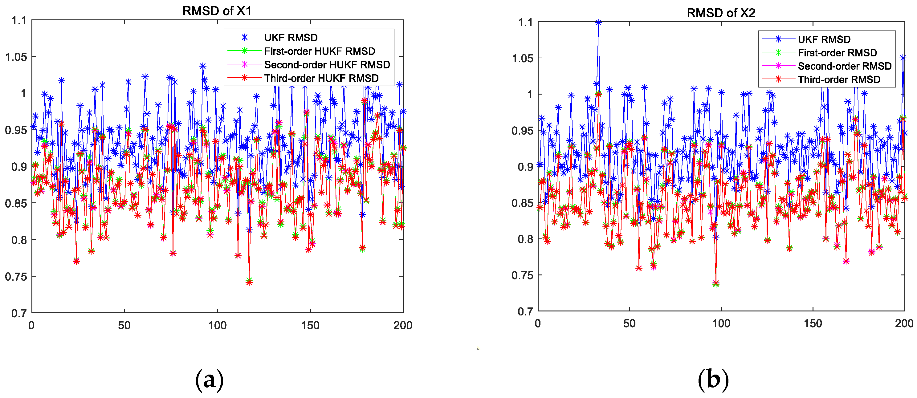
where the state noise and the measurement noise are both uncorrelated white Gaussian noise and obey the following distribution: w ( t ) N ( 0 , Q ) , v ( k ) N ( 0 , R ) , Q = d i a g ( 1 , 1 ) , R = d i a g ( 1 , 1 ) . The initial values of the system are x ( 0 ) = [ 1 , 1 ] , P ( 0 | 0 ) = I 2 × 2 . At the same time, the relevant parameters in the Unscented Transformation are set to α = 1 , β = 2 , λ = 1 and n = 2 . The simulation results are shown in the following figures. Figure 1a,b present the output curves of the true value of state X1 and state X2, the estimated value of the UKF, and the estimated value when the proposed filter is extended to the first and second orders. Figure 2a,b show the estimated error output results of the above filter in state X1 and state X2, respectively. Table 1 shows a comparison of the mean square error of each filtering method after the system is stabilized.
Through analysis of the data in the above table, it can be found that when the state equation is in the same dimension as the measurement equation, for equation X1, considering the first-order residual term information on the basis of the UKF improves the prediction accuracy by 6.50% compared with the traditional Unscented Kalman Filter. Considering the second-order remainder information on the basis of the UKF, the prediction accuracy is improved by 6.60% compared with the traditional Unscented Kalman Filter. and considering the third-order residual term information on the basis of the UKF, the prediction accuracy is improved by 6.61% compared with the traditional Unscented Kalman Filter. The prediction accuracy of the Unscented Kalman filtering method considering the second-order remainder information is 0.10% higher than that of the Unscented Kalman filtering method considering the first-order term information. The prediction accuracy of the Unscented Kalman filtering method considering the third-order remainder information is 0.01% higher than that of the Unscented Kalman filtering method considering the second-order term information.
For equation X2, considering the first-order residual term information on the basis of the UKF improves the prediction accuracy by 7.46% compared with the traditional Unscented Kalman Filter; considering the second-order remainder information on the basis of the UKF, the prediction accuracy is improved by 7.56% compared with the traditional Unscented Kalman Filter; and considering the third-order residual term information on the basis of the UKF, the prediction accuracy is improved by 7.56% compared with the traditional Unscented Kalman Filter. The prediction accuracy of the Unscented Kalman filtering method considering the second-order remainder information is 0.10% higher than that of the Unscented Kalman filtering method considering the first-order term information. The prediction accuracy of the Unscented Kalman filtering method considering the third-order remainder information is similar to that of the Unscented Kalman filtering method considering the second-order term information.
The second-order term information and third-order term information that can be extracted from the data-available residuals are already very sparse.

5.2. Simulation 2

The equation of state is two-dimensional nonlinear, and the measurement equation is one-dimensional linear.
x 1 ( k + 1 ) = 0.85 x 1 ( k ) + 0.5 x 2 ( k ) + 0.5 sin ( 0.5 x 1 ( k ) ) + w 1 ( k ) x 2 ( k + 1 ) = 0.5 x 1 ( k ) + 0.5 sin ( 0.5 x 2 ( k ) ) + w 2 ( k ) y ( k + 1 ) = x 1 ( k + 1 ) + 3 x 2 ( k + 1 ) + v ( k + 1 )
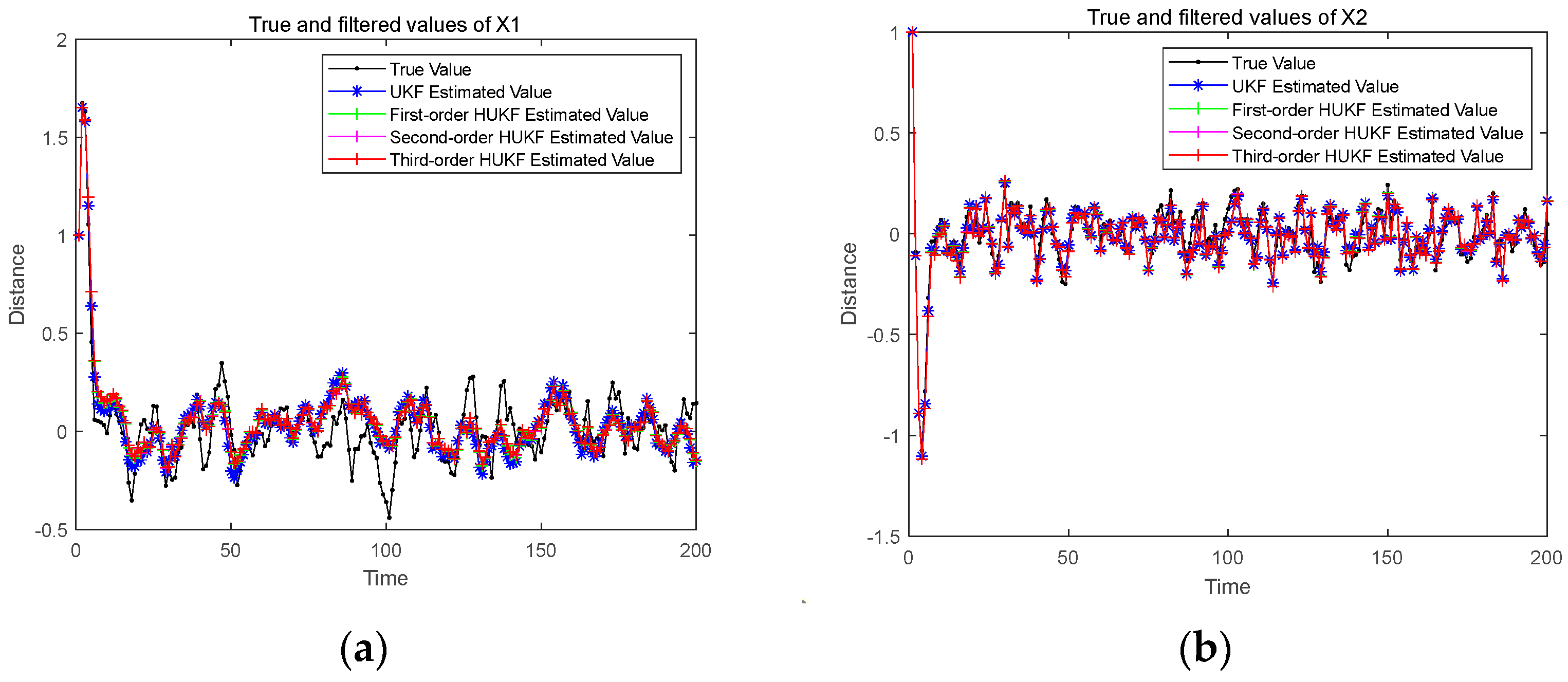
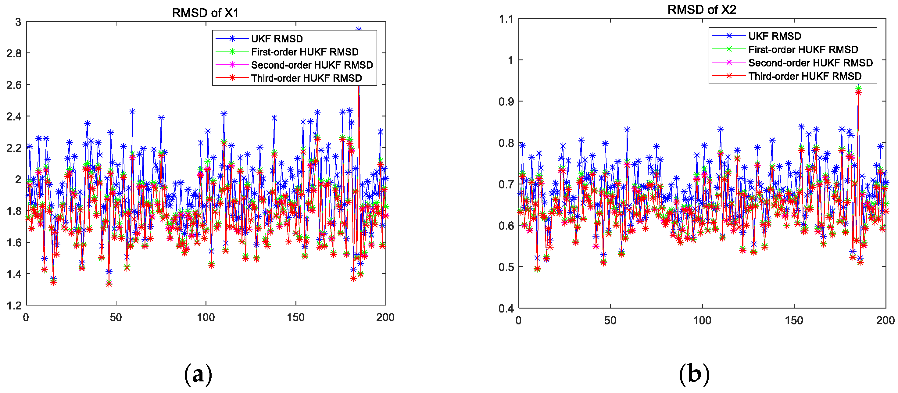
where the state noise and the measurement noise are both uncorrelated white Gaussian noise and obey the following distribution: w ( t ) N ( 0 , Q ) , v ( k ) N ( 0 , R ) , Q = d i a g ( 1 , 1 ) , R = 0.5 . The initial values of the system are x ( 0 ) = [ 1 , 1 ] and P ( 0 | 0 ) = I 2 × 2 . At the same time, the relevant parameters in the Unscented Transformation are set to α = 1 , β = 2 , λ = 1 , and n = 2 . The simulation results are shown in the following figures. Figure 3a,b present the output curves of the true value of state X1 and state X2, the estimated value of the UKF, and the estimated value when the proposed filter is extended to the first and second orders. Figure 4a,b show the estimated error output results of the above filter in state X1 and state X2, respectively. Table 2 shows a comparison of the mean square errors of each filtering method after the system is stabilized.
Through analysis of the data in the above table, it can be found that when the state equation and the measurement equation are not in the same dimension, for equation X1, considering the first-order residual term information on the basis of the UKF improves the prediction accuracy by 7.00% compared with the traditional Unscented Kalman Filter; considering the second-order residual term information on the basis of the UKF improves the prediction accuracy by 7.62% compared with the traditional Unscented Kalman Filter; and considering the third-order residual term information, the Unscented Kalman Filter improves the prediction accuracy by 7.70% compared with the traditional Unscented Kalman Filter. The Unscented Kalman Filter with second-order residual information improves the prediction accuracy by 0.62% compared with the Unscented Kalman Filter with first-order term information. The Unscented Kalman Filter with third-order residual information improves the prediction accuracy by 0.08% compared with the Unscented Kalman Filter with second-order term information.
For equation X2, considering the first-order residual term information on the basis of the UKF improves the prediction accuracy by 5.46% compared with the traditional Unscented Kalman Filter; considering the second-order residual term information on the basis of the UKF improves the prediction accuracy by 5.99% compared with the traditional Unscented Kalman Filter; and considering the third-order residual term information, the Unscented Kalman Filter improves the prediction accuracy by 6.06% compared with the traditional Unscented Kalman Filter. The Unscented Kalman Filter with second-order residual information improves the prediction accuracy by 0.53% compared with the Unscented Kalman Filter with first-order term information. The Unscented Kalman Filter with third-order residual information improves the prediction accuracy by 0.07% compared with the Unscented Kalman Filter with second-order term information.
In theory, as more error information is extracted and applied, the prediction accuracy increases. As the order increases, less information can be extracted, and the lifting effect will gradually weaken.

5.3. Summary of Simulation Results

Through analysis of the results of the above two simulation experiments, we can obtain the following conclusion:
Through analysis of the results of simulation 1, when the dimensions of the state equation and the measurement equation are 2 × 2 , it means that when the dimensions of the state equation and the measurement equation are the same dimension, from the perspective of observability (not observability in modern control), the degree of freedom of the equation is 0. For some equations, high-quality extraction of the remaining information can be completed by considering the first-order information of the remaining items on the basis of the UKF. The information in the second-order term and the third-order term is limited, and the improvement of the prediction accuracy is negligible.
Through analysis of the results of simulation 2, when the dimensions of the state equation and the measurement equation are 2 × 1 , it means that when the dimensions of the state equation and the measurement equation are different, this indicates under-measurement, and the degree of freedom of the equation is 1 from the perspective of observability. Therefore, it can be clearly found through the simulation data that the information in the first-order term, the information in the second-order term, and the information in the third-order term that can be extracted from the remainder is reduced. The prediction accuracy also decreases accordingly.
Through the above simulation experiments, the effectiveness of the new filtering method considering the high-order rejection error on the basis of the UKF is proved; through analysis of the dimensionality of the system’s state equation and the measurement equation, when the dimensionality is the same, the enhancement effect of the higher-order residual information on the prediction accuracy is minimal, and the first-order residual information can be extracted to achieve substantial enhancement of the prediction accuracy; when the dimensions are different, the enhancement effect of the higher-order residual information is more obvious than that of the same dimension. When the dimensions are different, the effect of higher-order residual information on the prediction accuracy is more obvious than that in the same dimension. For a system with two-dimensional state equations, one-dimensional measurement equations, and an operable degree of freedom of 1, the second-order residual information can be taken into account to achieve a substantial increase in the prediction accuracy, and this effect on the improvement of the prediction accuracy also increases with increasing under-measurement.

6. Conclusions

This paper improves the performance of nonlinear filtering based on Unscented Kalman filtering, fully considers the influence of high-order rejection error on the accuracy of state estimation, and improves the design issues of traditional Unscented Kalman filtering. A new filtering method considering high-order rejection errors based on Unscented Kalman filtering is established. The effectiveness of the proposed method is verified.
Outlook: Although the proposed method improves the filtering accuracy of the traditional UKF, there are still shortcomings. The proposed method is based on the fact that the state to be estimated is normally distributed, but the state to be estimated is often a non-Gaussian variable, which is difficult to conform to the normal distribution. Application of the proposed method to non-Gaussian distribution systems should be investigated in future studies. For non-Gaussian systems, further research is needed.

Author Contributions

Conceptualization, C.L. and C.W.; methodology, C.W.; software, C.L.; writing—original draft preparation, C.L.; writing—review and editing, C.L. All authors have read and agreed to the published version of the manuscript.

Funding

This work was supported by: (1) National Key R&D Program Intelligent Robot Key Special Project “Robot Joint Drive Control Integrated Chip” 2023YFB4704000; (2) National Natural Science Foundation of China 62125307, U22A2046, 61933013.

Institutional Review Board Statement

Not applicable.

Informed Consent Statement

Not applicable.

Data Availability Statement

Data are contained within the article.

Conflicts of Interest

The authors declare no conflicts of interest.

References

  1. Zhang, Z.; Zhang, Z.; Zhao, S.; Li, Q.; Hong, Z.; Li, F.; Huang, S. Robust adaptive Unscented Kalman Filter with gross error detection and identification for power system forecasting-aided state estimation. J. Frankl. Inst. 2023, 360, 10297–10336. [Google Scholar] [CrossRef]
  2. Kalman, R.E. A New Approach to Linear Filtering and Prediction Problems. J. Basic Eng. 1960, 82, 35–45. [Google Scholar] [CrossRef]
  3. Wen, C.; Cheng, X.; Xu, D.; Wen, C. Filter design based on characteristic functions for one class of multi-dimensional nonlinear non-Gaussian systems. Automatica 2017, 82, 171–180. [Google Scholar] [CrossRef]
  4. Wen, T.; Liu, J.; Cai, B.; Roberts, C. High-Precision State Estimator Design for the State of Gaussian Linear Systems Based on Deep Neural Network Kalman Filter. IEEE Sens. J. 2023, 23, 31337–31344. [Google Scholar] [CrossRef]
  5. Liu, X.; Wen, C.; Sun, X. Design Method of High-Order Kalman Filter for Strong Nonlinear System Based on Kronecker Product Transform. Sensors 2022, 22, 653. [Google Scholar] [CrossRef]
  6. Smith, G.L.; Schmidt, S.F.; McGee, L.A. Application of Statistical Filter Theory to the Optimal Estimation of Position and Velocity on Board a Circumlunar Vehicle; NASA Tech. Rep. TR R-135; National Aeronautics and Space Administration: Washington, DC, USA, 1962. [Google Scholar]
  7. Yue, M.; Zhe, G. Estimation for state of charge of lithium-ion batteries by adaptive fractional-order unscented Kalman filters. J. Energy Storage 2022, 51, 104396. [Google Scholar] [CrossRef]
  8. Cui, T.; Sun, X.; Wen, C. A Novel Data Sampling Driven Kalman Filter Is Designed by Combining the Characteristic Sampling of UKF and the Random Sampling of EnKF. Sensors 2022, 22, 1343. [Google Scholar] [CrossRef] [PubMed]
  9. Lee, A.S.; Hilal, W.; Gadsden, S.A.; Al-Shabi, M. Combined Kalman and sliding innovation filtering: An adaptive estimation strategy. Measurement 2023, 218, 113228. [Google Scholar] [CrossRef]
  10. Gustafsson, F.; Hendeby, G. Some Relations Between Extended and Unscented Kalman Filters. IEEE Trans. Signal Process. 2012, 60, 545–555. [Google Scholar] [CrossRef]
  11. Stepanov, O.A.; Litvinenko, Y.A.; Vasiliev, V.A.; Toropov, A.B.; Basin, M.V. Polynomial Filtering Algorithm Applied to Navigation Data Processing under Quadratic Nonlinearities in System and Measurement Equations. Part 1. Description and Comparison with Kalman Type Algorithms. Gyroscopy Navig. 2021, 12, 205–223. [Google Scholar] [CrossRef]
  12. Julier, S.J.; Uhlmann, J.K.; Durrant-Whyte, H.F. A new approach for filtering nonlinear systems. In Proceedings of the 1995 American Control Conference—ACC’95, Seattle, WA, USA, 21–23 June 1995. [Google Scholar]
  13. Juryca, K.; Pidanic, J.; Mishra, A.K.; Moric, Z.; Sedivy, P. Wind Turbine Micro-Doppler Prediction Using Unscented Kalman Filter. IEEE Access 2022, 10, 109240–109252. [Google Scholar] [CrossRef]
  14. Yang, F.; Zheng, L.; Wang, J.Q.; Pan, Q. Double Layer Unscented Kalman Filter. Acta Autom. Sin. 2019, 45, 1386–1391. [Google Scholar]
  15. Lei, Z.; Zidong, W.; Donghua, Z. Moving horizon estimation with non-uniform sampling under component-based dynamic event-triggered transmission. Automatica 2020, 120, 109154. [Google Scholar] [CrossRef]
  16. Juntao, W.; Jifeng, S.; Yuanlong, L.; Tao, R.; Zhengye, Y. State of charge estimation for lithium-ion battery based on improved online parameters identification and adaptive square root unscented Kalman filter. J. Energy Storage 2024, 77, 109977. [Google Scholar] [CrossRef]
  17. Cheng, C.; Wang, W.; Meng, X.; Shao, H.; Chen, H. Sigma-Mixed Unscented Kalman Filter-Based Fault Detection for Traction Systems in High-Speed Trains. Chin. J. Electron. 2023, 32, 982–991. [Google Scholar] [CrossRef]
  18. Mengli, X.; Yongbo, Z.; Huimin, F. Three-stage unscented Kalman filter for state and fault estimation of nonlinear system with unknown input. J. Frankl. Inst. 2017, 354, 8421–8443. [Google Scholar] [CrossRef]
  19. Stojanovski, Z.; Savransky, D. Higher-Order Unscented Estimator. J. Guid. Control Dyn. 2021, 44, 2186–2198. [Google Scholar] [CrossRef]
  20. Stepanov, O.A.; Isaev, A.M. A Procedure of Comparative Analysis of Recursive Nonlinear Filtering Algorithms in Navigation Data Processing Based on Predictive Simulation. Gyroscopy Navig. 2023, 14, 213–224. [Google Scholar] [CrossRef]
Figure 1. (a) The true and filtered values of X1. (b) The true and filtered values of X2.
Actuators 13 00169 g001
Figure 2. (a) X1 RMSD of various methods. (b) X2 RMSD of various methods.
Actuators 13 00169 g002
Figure 3. (a) True values and filtered values of X1. (b) True values and filtered values of X2.
Actuators 13 00169 g003
Figure 4. (a) RMSD of X1. (b) RMSD of X2.
Actuators 13 00169 g004
Table 1. Performance comparison of various methods.
StateRMSD of X1RMSD of X2
Methods
UKF0.9367640.926681
First-order estimate0.8759190.857522
Improvement6.50%7.46%
Second-order estimate0.8748970.856663
Improvement6.60%7.56%
Third-order estimate0.8748170.856622
Improvement6.61%7.56%
Table 2. Performance comparison of different algorithms.
StateRMSD of X1RMSD of X2
Methods
UKF1.934160.683426
First-order estimate1.798710.646101
Improvement7.00%5.46%
Second-order estimate1.786690.642469
Improvement7.62%5.99%
Third-order estimate1.785240.642038
Improvement7.70%6.06%
Disclaimer/Publisher’s Note: The statements, opinions and data contained in all publications are solely those of the individual author(s) and contributor(s) and not of MDPI and/or the editor(s). MDPI and/or the editor(s) disclaim responsibility for any injury to people or property resulting from any ideas, methods, instructions or products referred to in the content.