Magnetic Performance of Eddy Current Suppressing Structures in Additive Manufacturing

Abstract

Additively manufactured soft-magnetic components are inherently bulky leading to significant eddy current losses when applied to electrical machines. Prior works have addressed this issue by implementing structures based on the Hilbert space-filling curve which include eddy current suppressing gaps, thereby reducing the fill factor of the soft-magnetic component. The present research aims at investigating a number of space-filling curves in addition to sheets in order to find the optimal eddy current suppressing structure from an electromagnetic point of view. By means of both analysis and finite-element simulation, it was shown that sheets are superior at minimizing eddy current losses while space-filling curves excel at maximizing the fill factor.

1. Introduction

Additive manufacturing (AM) is a technique experiencing fast adoption in prototyping and low-volume manufacturing. Its main benefit is the ability to directly use a computer-aided design (CAD) model which results in fast design iteration and the possibility to create complex geometries in a single part [1]. Additionally, material waste is greatly reduced compared to subtractive manufacturing techniques, which instead currently excel in high-volume production.

Although the span of AM components already ranges from purely mechanical ones [2] to functional use such as with electronics [3] and radio frequency components [4,5], the investigation of many potential applications such as magnetic flux-guiding components has only recently started [6]. The first application of this kind was the core of a transformer by Plotkowski et al. in [7]. A more recent set of publications by Goodall et al. presented an axial flux machine with an additively manufactured stator [8,9]. Both of these research groups already addressed one of the main issues with AM-built soft-magnetic components, namely eddy currents and their respective losses.

As the AM process is intrinsically bulky due to the deposition of one layer on top of the other, the lack of electrical insulation enables eddy currents to flow freely, resulting in unobstructed power losses already at low frequencies and consequently thermal issues for the entire electrical machine. In classical manufacturing of these soft-magnetic components, thin insulated sheets are cut to the required geometry and then stacked on top of each other. Thus, the eddy currents are limited to the width of a single sheet. However, this process is tedious and expensive, which are exactly some reasons one might choose AM processing in the first place. A similar approach can be implemented by only filling regions of the bulk component, leaving gaps between them [10]. Naturally, the gaps should be as narrow as possible while still insulating the regions from each other. However, there are additional aspects to consider. In the case of powder bed processes, which is the AM process used in both [7,8], the gaps are still filled with powder once the component is finished. Thus, the gaps have to be wide enough for the powder to be removable or the component will once again be quasi-bulky from an electromagnetic point of view. Additionally, the surfaces of AM-built components are quite rough compared to conventionally manufactured parts [11]. If such surfaces are very close to each other inside a component, it is very likely that they are connected at a number of points. These aspects have to be considered when choosing the minimum viable gap size. An in-depth investigation of Fe-6.5 wt%Si on this latter issue is presented in [8] resulting in a minimum gap size of $50\mathsf{\mu }\mathrm{m}$ with the gap plane perpendicular to the build plane and $250\mathsf{\mu }\mathrm{m}$ when the build and gap planes are parallel to each other. These values may be reduced by improving both the alloy properties and AM process but still represent non-negligible regions of the soft-magnetic component which are not soft-magnetic.

Structures already applied by different research groups in order to reduce the eddy current losses range from interconnected sheets [12] to hexagons [13] and clock springs [7]. Despite this, every research group has ultimately chosen to use a so-called space-filling curve (SFC). 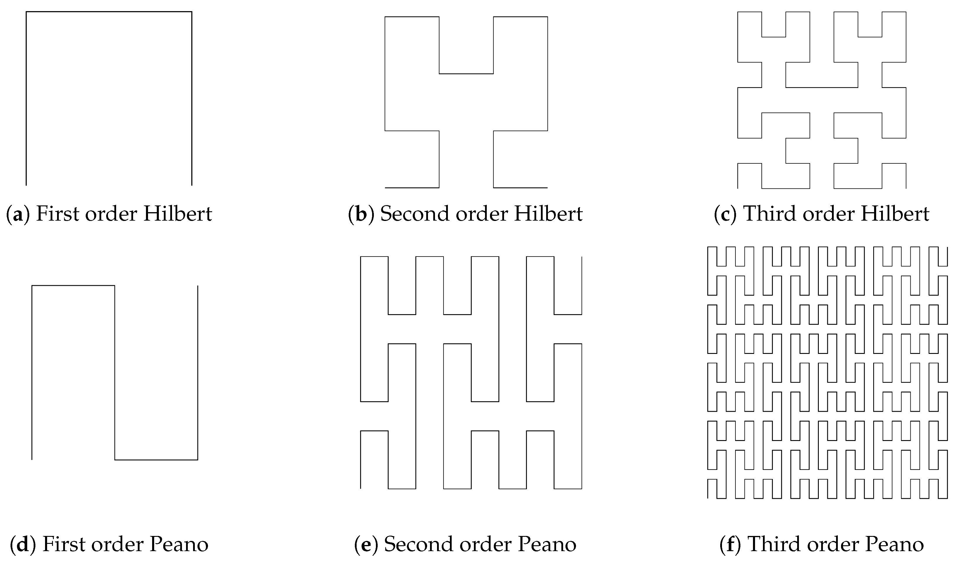SFCs were originally investigated in mathematics with the idea of filling an area or a volume using a one-dimensional object [14]. In order to achieve this property, fairly simple geometries are refined over a theoretically unlimited number of iterations according to rules specifically designed for the appropriate SFC, similar to the creation of fractals. A small number of iterations for the Hilbert and Peano SFCs are shown in Figure 1. Over time, a number of SFCs were developed such as the already mentioned Hilbert and Peano curves but also the Moore curve, Lebesgue curve, Sierpiński curve and many more [15]. Practical applications of SFCs mainly concern informatics: Their property of creating a continuous path on higher dimensional objects is used in processing or compressing images and optimizing search algorithms [16,17]. One of the most important properties for these operations is locality, that is, the ratio of distance between points in the respective space to the distance of these points along the SFC [18]. However, this aspect is yet to be connected to magnetic performance and will therefore not be included in the presented research.

Another characteristic influencing eddy current losses is the width of the structures between the insulating gaps, similar to the thickness of sheets in laminated soft-magnetic components. In order to achieve minimal power losses, the minimum manufacturable thickness should be implemented. However, this increases the number of gaps and consequently the gap volume. Thus, this approach reduces the fill factor and subsequently the maximum magnetic flux which the component can guide. Therefore, a compromise between eddy current losses and fill factor has to be made. The topic of fill factor is also especially interesting, as research on soft-magnetic metal-polymer composites has shown a strong non-linear connection between fill factor and magnetic properties as well as losses [19,20,21].

This paper provides insight into the magnetic performance of a number of eddy current limiting structures and compares them regarding both their resulting power loss density due to eddy currents as well as fill factor of soft-magnetic material. Section 2 recaps eddy current losses in thin sheets and introduces the finite-element (FE) model used in the investigation. Section 3 presents the eddy current losses of structures based on so-called space-filling curves (SFCs) and compares the respective results with the losses of similarly sized sheets. The fill factors of the presented structures are compared in Section 4, and Section 5 summarizes the conclusions of the research.

2. Eddy Current Losses in Sheets

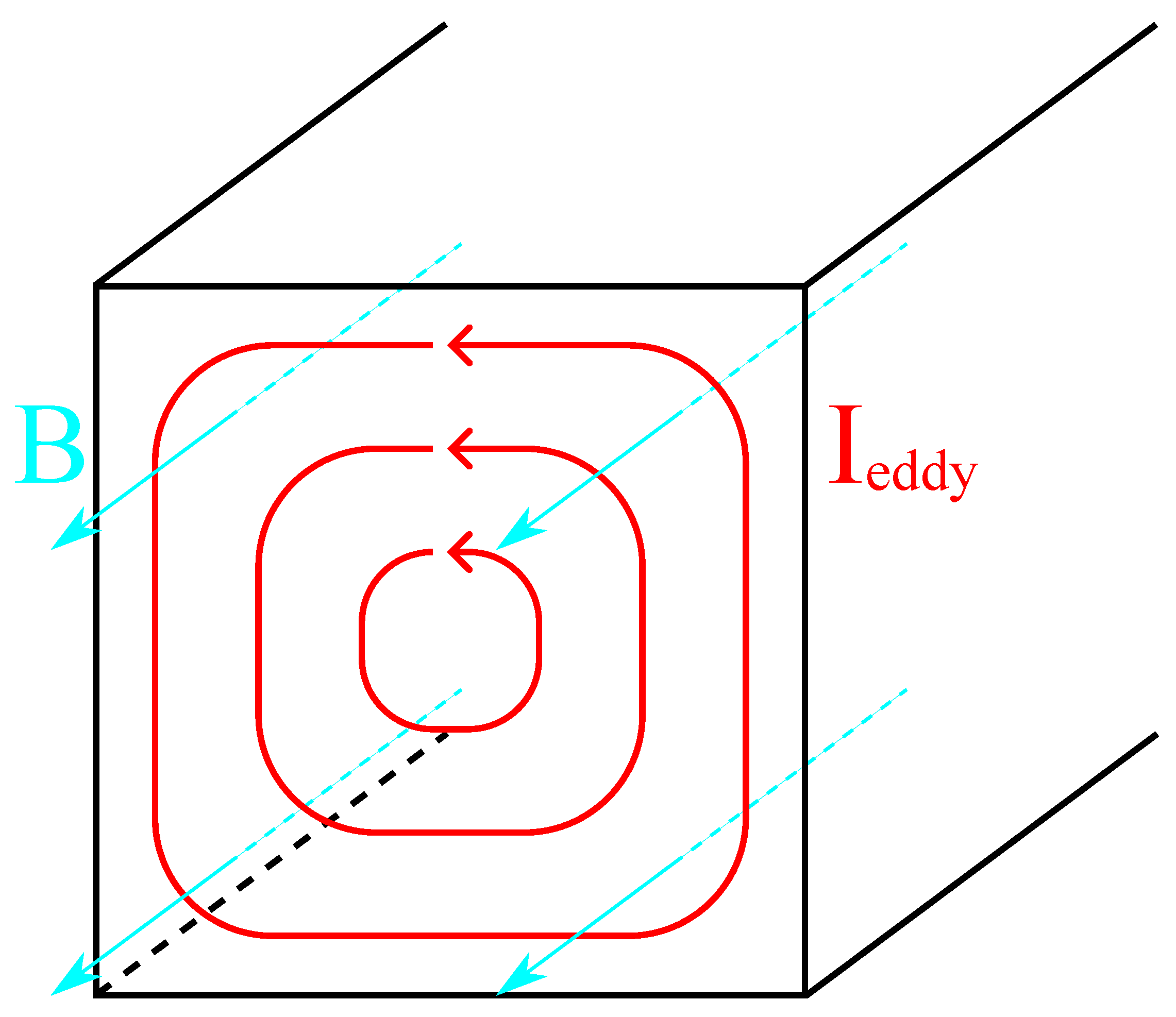
Eddy currents are electrical currents induced in electrically conductive materials experiencing a change in magnetic field. The cause of this change may be due to the magnetic field changing, e.g., by driving a nearby coil with a sinusoidal source, or by the material itself moving within a static magnetic field. As portrayed in Figure 2, this induced current $I_{eddy}$ circulates in a plane perpendicular to the magnetic flux denoted by the flux density B. The current leads to ohmic losses and therefore generates heat in materials with non-zero electrical resistivity ${\rho }_{el}$. Additionally, this current generates a magnetic field itself which may distort the applied magnetic field. Although eddy currents are useful in some applications such as eddy current brakes [22], in most other applications they are undesired and means to suppress eddy currents and subsequent losses are implemented. The most common method to reduce eddy current losses is by using electrically insulated and stacked soft-magnetic sheets instead of bulk components.

A general formulation for both eddy currents and their losses have been derived in literature such as [23] but are omitted here for reasons of brevity. Instead, a simplified estimation for eddy current losses in thin sheets of thickness d in m experiencing a sinusoidal magnetic field of frequency f in Hz as presented in [24] will be used:

$$\begin{array}{c}\hfill W=\frac{{\pi }^2{d}^2{B}_p^{2}f}{6{\rho }_{el}{\rho }_m},\end{array}$$

(1)

where W is the specific loss per cycle in $\frac{\mathrm{J}}{\mathrm{kg}}$, $B_p$ the peak magnetic flux density in T and ${\rho }_m$ the volumetric mass density of the material in $\frac{\mathrm{kg}}{{\mathrm{m}}^3}$. The specific power lost P in $\frac{\mathrm{W}}{\mathrm{kg}}$ can be expressed as:

$$\begin{array}{c}\hfill P=Wf=\frac{{\pi }^2{d}^2{B}_p^2{f}^2}{6{\rho }_{el}{\rho }_m}.\end{array}$$

(2)

These equations already show the effect of using thin sheets, as the square of their thickness d is directly linked to P. Although this leads to the objective of minimizing d, there is a practical limit to the thickness of sheets concerning both cost of production and handling of such sensitive parts. Thus, most providers limit their regular product at around $d=0.1\mathrm{mm}$ with thinner sheets being available for a markup.

Inserting some thicknesses d into (2) using the values presented in

Table 1. Parameters used for analytical and FE simulation determination of eddy current losses.

Parameter	Symbol	Value
Frequency	f	$10\mathrm{Hz}$
Peak Flux Density	$B_p$	$1\mathrm{T}$
Electrical Resistivity	${\rho }_{el}$	$89.29\mathrm{n}\mathsf{\Omega }\mathrm{m}$
Relative Magnetic Permeability	${\mu }_r$	4000
Volumetric Mass Density	${\rho }_m$	$7870\frac{\mathrm{kg}}{{\mathrm{m}}^3}$
Cube Side Length	l	$1\mathrm{mm}$

leads to the specific power losses listed in

Table 2. Specific eddy current losses for sheets of different thickness d.

d in mm	Specific Power Losses P in $\frac{\mathbf{mW}}{\mathbf{kg}}$
	Analytical	2D Analytical	FE Simulation
1	234.09	117.05	97.84
0.5	58.52	46.82	40.01
0.25	14.63	13.77	12.33
0.1	2.34	2.32	2.20

under ’Analytical’.

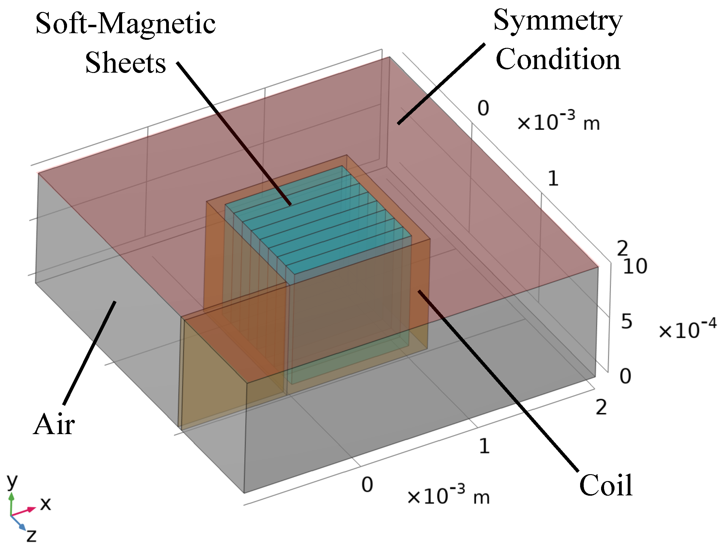
Table 2 additionally contains loss values determined by means of FE simulation using COMSOL Multiphysics as well as ’2D Analytical’ results which will be explained later. As illustrated in Figure 3, the soft-magnetic component simulated is a cube with side length $l=1\mathrm{mm}$ which itself is comprised of stacked sheets of the appropriate thickness d. Instead of using a finite gap for electrical insulation, the sheets are electrically insulated by 2D planes with ${\rho }_{el}=\infty \mathsf{\Omega }\mathrm{m}$. Thus, the specific power loss can be calculated by dividing the total loss in the cube by its volume and mass density. The cube is surrounded by electrically non-conducting air on four sides as well as a homogenized multi-turn coil whose current is adjusted on a per model basis in order to create the magnetic flux density according to Table 1. The two parallel planes of the open sides of the cube have boundary conditions applied which only allow B-fields perpendicular and currents parallel to the respective plane. Thus, the cube is modeled as a section of a long beam without any end effects, reducing computational cost and time substantially and introducing negligible deviation from a real-life configuration exhibiting end effects.

The latter assumption is especially helpful as (2) is based on an infinitely large sheet of thickness d. However, the FE model only applies an infinite length in one dimension instead of two which contributes to the significant deviations of results in Table 2. This error can be reduced by extending the square in its x-axis direction such that $l>>d$ but this leads to highly increased computational time and, most importantly, deviates from the square shape of the cross section. The reason for this square shape will become obvious in Section 3 and with the introduction of SFCs. Their resulting structures are inherently square-shaped which requires the sheets to also fill this shape for a one-to-one comparison.

Instead, (2) is extended as suggested in [25] in order to include the length of the sheet:

$$\begin{array}{c}\hfill P=\frac{{\pi }^2{d}^2{l}^2{B}_p^2{f}^2}{6\left(d^2+l^2\right){\rho }_{el}{\rho }_m}.\end{array}$$

(3)

As (3) simplifies into (2) for $l>>d$, it covers all sheet lengths and will therefore be used for all future calculations. The results of this equation are reported in the column ’2D Analytical’ of Table 2 and are significantly closer to the ones obtained by means of FE analysis especially for the cases where d is close to l.

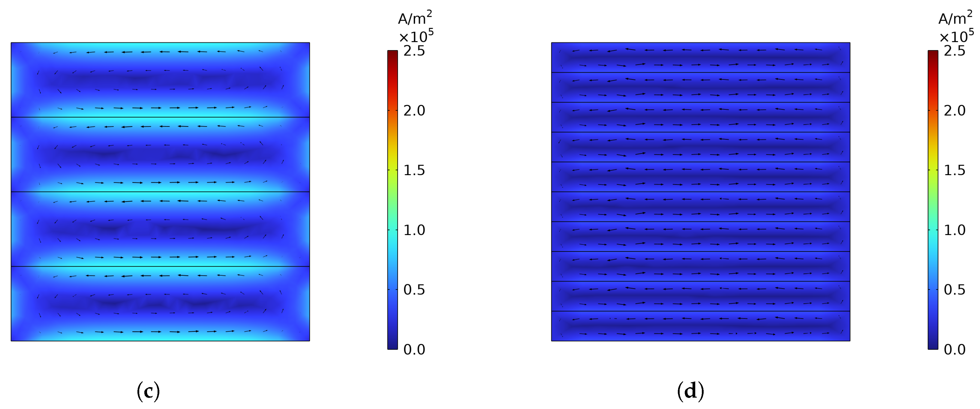
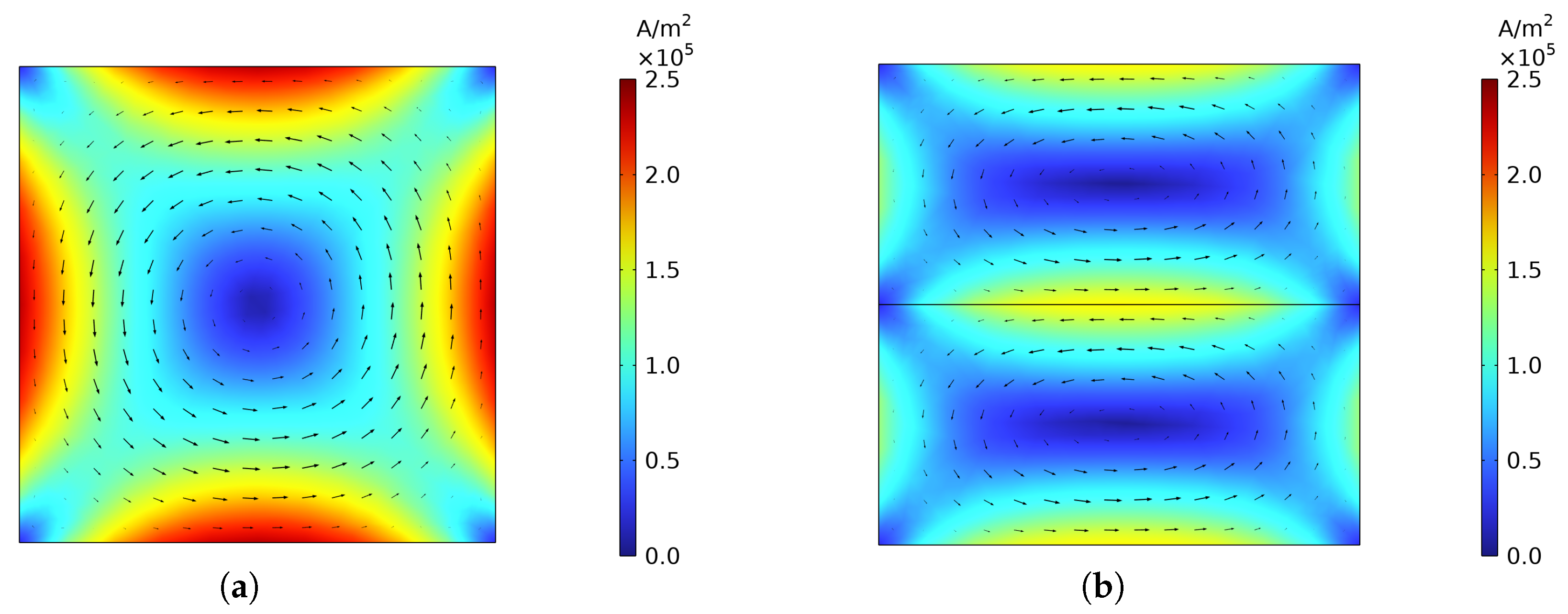
Figure 4 illustrates the flux density of the cube obtained by FE analysis for $d\in \{1,0.5,0.25,0.1\}\mathrm{mm}$ while the current density is presented in Figure 5. These figures show an additional aspect of eddy currents omitted until now, namely the skin effect. As indicated by both the coloring and the arrow size of Figure 5, the current density tends to be high at the edges of the sheets and near zero at their center. This has consequences for the effective cross section of electrical conductors especially at high frequencies but also affects the flux density distribution in magnetic conductors as indicated in Figure 4. In fact, the flux density is anisotropic for all models, yet it is less so for thin sheets as the standard penetration depth $\delta$ of the current is constant for all sheet thicknesses [26]:

$$\begin{array}{c}\hfill \delta =\sqrt{\frac{{\rho }_{el}}{\pi f\mu }}=0.752\mathrm{mm},\end{array}$$

(4)

where $\mu ={\mu }_0{\mu }_r$ is the magnetic permeability of the material. The skin effect also explains the remaining deviation between the analytical and simulation results in Table 2 as (2) and (3) assume a constant flux density across the whole sheet while the targeted peak flux density of $B_p=1\mathrm{T}$ is only achieved as a mean value in simulation. This is also reflected in the fact that the relative error increases with d and the magnetic flux density approaches a virtually constant value for the entire soft-magnetic component in simulation for $d=0.1\mathrm{mm}$.

3. Space-Filling Curves

Although there are a large number of SFCs, only two SFCs, the Hilbert and Peano curves, were chosen for this investigation in which the magnetic performance will be compared against sheets. These two SFCs, and especially the Hilbert curve, are also the ones used in studies such as [7,8,9,13]. The main reasons for excluding other SFCs are either that they do not fill a unit square which can then be replicated and adjusted to fit any area, they are too similar to another SFC, such as the Moore curve to the Hilbert curve, or they cannot be manufactured with a finite width without simplifying them beyond recognition, for example the Lebesgue curve. Figure 6 shows the two chosen SFCs and their resulting cross sections used for FE simulation. This figure also includes the Sierpiński curve to illustrate that not every SFC is a reasonable choice for application purposes.

As shown in Figure 6c, the Sierpiński curve cannot simply be widened to fill a finite area without creating short circuits. Thus, in order to avoid a significantly reduced fill factor, its geometry would have to be adapted, as illustrated in Figure 6f. Upon further inspection, the resulting cross section is mainly made of triangles. As triangles must always have at least two acute angles, manufacturing this structure, while respecting any minimum viable structure width, will always fail at these corners and either create short circuits or reduce the fill factor once again. Thus, also this variant of the Sierpiński curve is not a worthwhile choice.

For each of the selected SFCs (Hilbert and Peano), the first three orders were investigated. As mentioned previously, the minimum reliably manufacturable gap $w_g$ for Fe-6.5 wt%Si was found to be $50\mathsf{\mu }\mathrm{m}$ for gaps parallel to the build direction with wider gaps required in other orientations [8]. In order to simplify the calculations, only gaps perpendicular to the build plane will be considered such that a constant $w_g=50\mathsf{\mu }\mathrm{m}$ can be applied everywhere. The nominal structural width w was chosen to be $0.5\mathrm{mm}$ as this structure width is the minimum width $w_{min}$ known to be manufacturable [8]. As the parameters of Table 1 are applied also for these soft-magnetic components, the penetration depth of $\delta =0.752\mathrm{mm}$ applies here, too. Since this value is close to the chosen $w_{min}=0.5\mathrm{mm}$ some skin effect is to be expected. The assumptions made lead to predetermined cross sections for each order of SFC, as shown in Figure 7 for the Hilbert curve. Analog to the sheets, the coil current is adapted for each SFC to achieve a mean peak flux density of $1\mathrm{T}$. 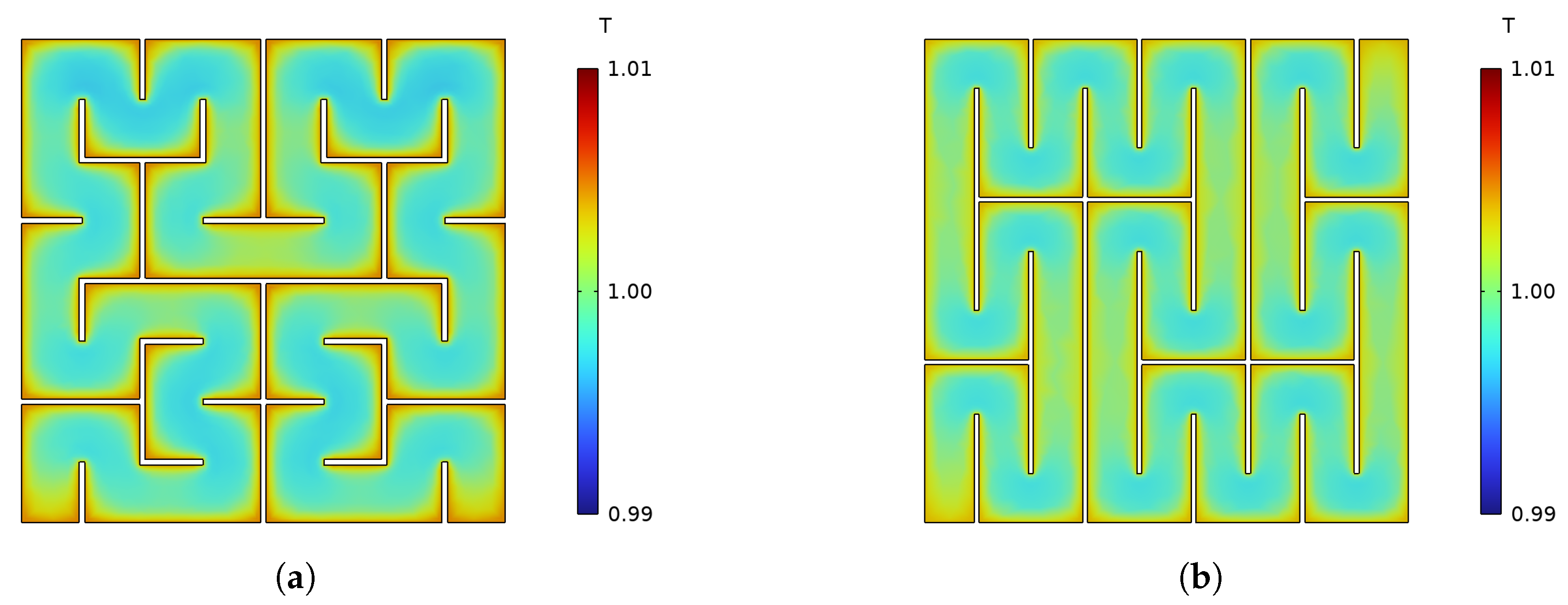The resulting flux density distribution of select SFCs is shown in Figure 8 with the current density presented in Figure 9.

Similarly to Figure 4, the flux densities shown in Figure 8 are inhomogeneous. However, there is a clear difference between regions which are mostly straight and ones characterized by corners. This difference can once again be explained using (4). Although the nominal thickness is constant for all regions, the effective cross section of corners is greater than that of straight regions. Therefore, the constant penetration depth leads to a higher heterogeneity of flux density in corners.

Inspecting the current density, one can spot that there are local effects around sharp corners due to singularities. The finite element mesh at these points was refined in order to confine the affected area. However, they likely still introduce some error. Nevertheless, by integrating the specific losses and dividing them by the volume and volumetric mass density ${\rho }_m$ of the soft-magnetic component, the specific eddy current losses can be estimated as presented in

Table 3. Specific eddy current losses for a number of different SFCs.

SFC & Order	Specific Losses P in $\frac{\mathbf{mW}}{\mathbf{kg}}$
	FE Simulation	Analytical $\mathit{w}$	Analytical $\overline{\mathit{w}}$
Hilbert 1	56.22	55.52	66.73
Hilbert 2	66.16	58.33	79.97
Hilbert 3	71.64	58.51	81.47
Peano 1	60.44	57.92	69.26
Peano 2	64.41	58.52	71.67
Peano 3	64.97	58.52	71.84

.

Analytically validating the results for eddy current losses of these models is not straight forward as equations such as (3) assume a constant sheet thickness d, which is not the case for the SFCs portrayed in Figure 6. Nonetheless, by inserting the nominal width w for d and length $l_{SFC}$ of the SFCs for l into (3), the losses can be estimated and are provided in the ’Analytical w’ of Table 3. These results are fairly close to the ones obtained by means of FE simulation. However, they fail to replicate the significant differences between the orders of the SFCs, sometimes predicting higher and sometimes lower losses than the FE simulation. This also contradicts the values of Table 2 where the analytical results for sheets are always higher than the ones obtained by means of FE simulation.

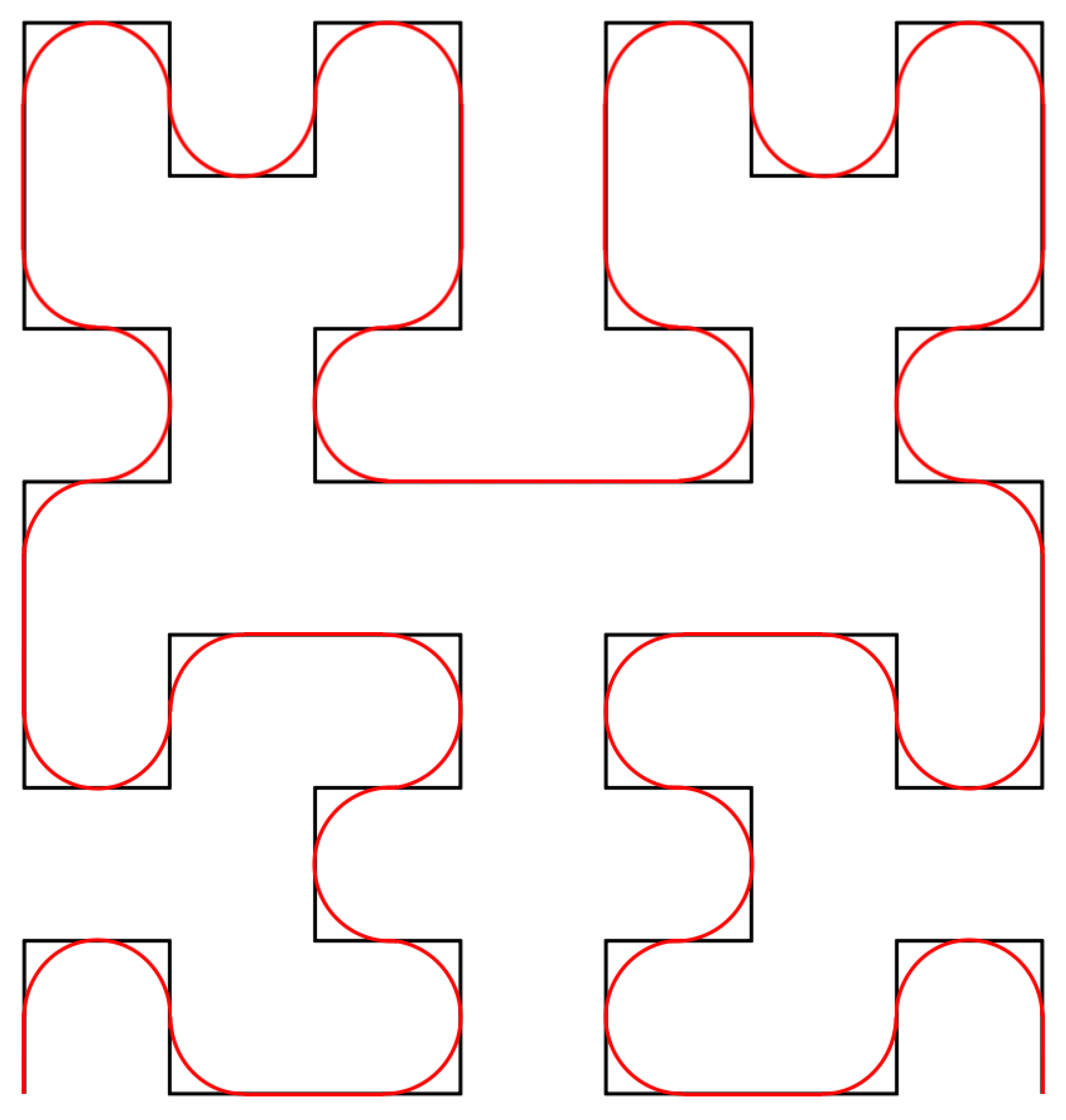
A significant source of this error can be extracted from Figure 8 and Figure 9. These figures clearly show that both the magnetic flux and the current do not follow the SFCs as derived analytically and shown in Figure 10 in black but rather arc at every corner. Estimating these arcs as illustrated in Figure 10 in red leads to a new curve length $l_{SFC}^{*}$. This effective length $l_{SFC}^{*}$ is smaller than $l_{SFC}$ leading to an increased mean width $\overline{w}$ calculated as:

$$\begin{array}{c}\hfill \overline{w}=\frac{A_{eff}}{l_{SFC}^{*}},\end{array}$$

(5)

where $A_{eff}$ is the effective soft-magnetic area which will be derived for the investigated SFCs in Section 4.

The respective loss densities are included in the last column of Table 3 ’Analytical $\overline{w}$’. These analytical results always show a higher loss density than the ones obtained by means of FEA. Moreover, the ratio of results obtained by means of FE simulation to the ones obtained by using $\overline{w}$ and $l_{SFC}^{*}$ is quite consistent across the different SFCs and their orders.

It is also of interest to investigate the remaining deviation as to potentially develop models which predict the eddy current losses more accurately. For this purpose, the first three iterations of the Hilbert curve have been examined using $w\in \left[0.1;0.2;0.5\right]\mathrm{mm}$, $w_g\in \left[0.01;0.05;0.1\right]\mathrm{mm}$ and $f\in \left[10;50;200\right]\mathrm{Hz}$. Inspecting the resulting loss densities leads to the conclusion that the deviation mainly depends on the geometry of the respective SFC. The resulting ratio of loss densities are illustrated in Figure 11 with the x-axis defined by a geometric ratio $\gamma$

$$\begin{array}{c}\hfill \gamma ={\left(\frac{\overline{w}}{l_{SFC}^{*}}\right)}^{\frac{1}{o}},\end{array}$$

(6)

thus also taking into account the order o of the SFC. The lines are functions obtained by fitting the data points not showing a significant skin effect.

The deviation in the results that do show a significant skin effect is straight forward as the analytical results do not include this effect. Nevertheless, these loss ratios appear to decrease systematically as illustrated in the bottom right corner of Figure 11. These nine points represent the most extreme case of skin effect investigated ($w=0.5\mathrm{mm}$ and $f=200\mathrm{Hz}$) and are shifted down from their low-frequency counterparts.

Focusing on the remaining results, one can see that there are clusters of multiple points that are slightly shifted along the y-axis. The difference between these points is the applied frequency. Therefore, these results experience a slight skin effect as well. However, this also implies that the frequency does not contribute to the loss ratio apart from this effect. Therefore, the loss ratios do depend on the geometric parameters themselves.

Inspecting the different orders, they each appear to create their own trend line with an increasingly negative slope as the order increases. This is likely related to the number of edges introduced into the geometry as this aspect is the main difference between them. For large geometric ratios, the loss ratio of the first order Hilbert curve appears to saturate whereas the second order Hilbert curve only starts to flatten in the provided data set. The exact reasons for this systematic error are still unclear and necessitate an in-depth investigation. It appears that the applied analytical model is incomplete and has to be extended in order to correctly model these structures. Nevertheless, the applied model consistently overestimates the losses, making preliminary calculation situationally useful.

Comparison with Sheets

In order to compare the sheet loss densities to the ones of the SFCs, the number of sheets N and their length l is adjusted in order to fill the same area as the cube filled by the SFC.

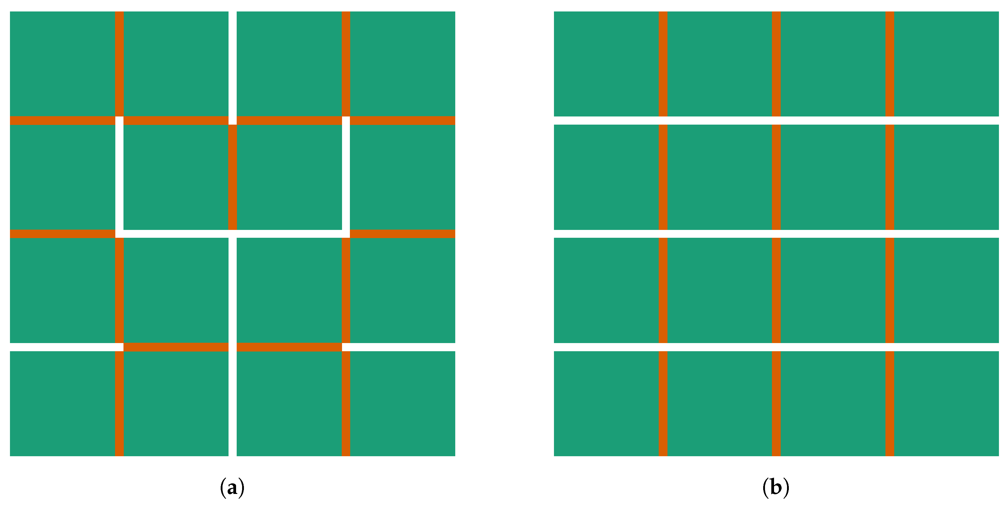
Therefore a modelling approach is introduced which is illustrated in Figure 12 for the second order of the Hilbert curve and the respective packaged sheets as an example. Depending on the order o of the Hilbert curve, a grid of $2^o$ by $2^o$ of squares is generated, thus, a 4 by 4 grid for the case depicted in Figure 12. These squares have a side length equal to the nominal structural width w. The gap between neighbouring squares is of width $w_g$. By strategically filling these gaps with rectangles of size w by $w_g$, either the Hilbert structure or the sheet-based structure can be generated. Consequently, the nominal structural width w of the SFC and the sheet thickness d are the same with $w=d=0.5\mathrm{mm}$. The number of sheets N required and the length l of the sheets depend on the order o and can be calculated by means of

$$N=2^o,$$

(7)

$$l=2^{o}w+(2^o-1)w_g.$$

(8)

The Peano curve and a sheet-based component of the same area can be modeled analogously with slight changes to the equations as each side is split into three parts per iteration instead of two:

$$N=3^o,$$

(9)

$$l=3^{o}w+(3^o-1)w_g.$$

(10)

Inserting these values into (3) leads to the loss densities in

Table 4. Specific eddy current losses obtained analytically and via FE simulation for a number of different SFCs and sheets of thickness $d=w$.

SFC & Order	Specific Losses P in $\frac{\mathbf{mW}}{\mathbf{kg}}$
	Analytical		FE Simulation
	SFC	Sheets	SFC	Sheets
Hilbert 1	66.73	47.71	56.21	40.97
Hilbert 2	79.97	55.52	66.16	49.89
Hilbert 3	81.47	57.76	71.64	54.22
Peano 1	69.26	53.32	60.44	46.96
Peano 2	71.67	57.92	64.41	54.70
Peano 3	71.84	58.46	64.97	57.32

, which also includes the loss densities for the same structures obtained by means of FE simulation.

Although the before mentioned differences between the results obtained by analysis and FE simulation are yet to be considered, both methods show the same overall result, namely significantly lower specific losses for sheets. Nevertheless, the discussion of the results will focus on the ones obtained by means of FE simulation notwithstanding the fact that the reduction in losses are in the same range.

Compared to the Hilbert SFCs, sheets exhibit $24\%$ to $27\%$ lower loss densities while being between $12\%$ and $22\%$ lower than that of the Peano SFCs. This consistent improvement concerning eddy current losses is quite significant, making sheets an attractive form of loss reduction. Some implications this loss reduction leads to are that a SFC-based structure has to be manufactured about $10\%$ thinner in order to show the same loss density or that the sheet-based structure can be wider and thus fill a larger area while achieving similar loss densities. An additional benefit of sheets is that they are based on straight lines instead of an already fixed structure. These lines can be easily adjusted to, for example, fill a circular structure such as a rotor of an electrical machine. Nevertheless, this result is only useful in application if a reduction in fill factor of the sheets due to insulating gaps is not too significant.

4. Fill Factor Comparison

So far the main focus of the present research was eddy current losses, and it was shown that sheets of the same width always exhibit lower losses than the investigated SFCs. However, another important aspect is the fill factor

$$\begin{array}{c}\hfill F=\frac{V_{eff}}{V_{total}},\end{array}$$

(11)

defined as the ratio of the effectively usable soft-magnetic volume $V_{eff}$ to the total volume $V_{total}$ such that

$$\begin{array}{c}\hfill V_{eff}=V_{total}-V_{gap}.\end{array}$$

(12)

Since F is directly linked to the maximum magnetic flux, maximizing it will increase the power density of the electrical machine.

As in the investigation of the loss densities, the gap width $w_g$ is assumed to be constant. In order to guarantee manufacturability, the components are obtained by extruding a 2D structure and, instead of using $V_{eff}$ and $V_{total}$, the effective area $A_{eff}$, gap area $A_{gap}$ and total area $A_{total}$ are introduced such that

$$\begin{array}{c}\hfill V_{eff}=A_{eff}h,\end{array}$$

(13)

$$\begin{array}{c}\hfill V_{gap}=A_{gap}h,\end{array}$$

(14)

$$\begin{array}{c}\hfill V_{total}=A_{total}h,\end{array}$$

(15)

$$\begin{array}{c}\hfill A_{eff}=A_{total}-A_{gap}\end{array}$$

(16)

where h represents an arbitrary build height. This allows the comparison of the fill factor F by means of

$$\begin{array}{c}\hfill F=\frac{A_{eff}}{A_{total}},\end{array}$$

(17)

which should be maximized. In the case of laminated sheets of thickness d, the effective area, gap area and total area are calculated as

$$\begin{array}{c}\hfill A_{eff,sheets}=Nld,\end{array}$$

(18)

$$\begin{array}{c}\hfill A_{gap,sheets}=Nl{w}_g,\end{array}$$

(19)

$$\begin{array}{c}\hfill A_{total,sheets}=Nld+Nl{w}_g,\end{array}$$

(20)

with l being an arbitrary side length. In this case, the gap is insulation due to the sheets being insulated before cutting and stacking them. However, at the aim of simplifying manufacturing, AM-built sheet-based components should be printed as extruded lines of thickness d with air gaps of thickness $w_g$ serving as insulation between them. Thus, there is no insulation at the outer edges of the component. This leads to a modified equation of $A_{gap,sheets}$ and consequently to

$$\begin{array}{c}\hfill A_{total,\mathit{\text{AM-sheets}}}=Nld+(N-1)l{w}_g.\end{array}$$

(21)

As one can see, the only difference is that the number of insulation gaps is reduced by one. Inserting these expressions into (17) leads to:

$$\begin{array}{c}\hfill F_{\mathit{\text{AM-sheets}}}=\frac{A_{eff,sheets}}{A_{total,\mathit{\text{AM-sheets}}}}=\frac{Nd}{Nd+(N-1)w_g},\end{array}$$

(22)

$$\begin{array}{c}\hfill F_{sheets}=\frac{A_{eff,sheets}}{A_{total,sheets}}=\frac{d}{d+w_g}.\end{array}$$

(23)

Inspecting these two fill factors it is clear that their difference decreases with an increasing number of sheets N as presented in Figure 13.

Figure 14 shows $F_{sheets}$ for a commonly available range of sheet thicknesses d as well as a variety of gap widths $w_g$. As $F_{sheets}$ is independent of N and l, the actual geometry is irrelevant. Instead, this figure illustrates the significant impact of $w_g$ on the fill factor. Using $w_g=50\mathsf{\mu }\mathrm{m}$, as indicated by the green line in Figure 14, thick sheets have to be used in order to achieve reasonable fill factors above $0.9$. These thicker sheets would naturally increase the eddy current losses. Conventionally manufactured packaged sheets are more in line with the blue line, $w_g=10\mathsf{\mu }\mathrm{m}$, and show high fill factors even for quite small d. Therefore, considerable improvements to AM-processing are required for achieving similar fill factors.

As the presented investigation concerns additive manufacturing, the sheet thickness d may vary depending on the desired geometry. With the aim of simplifying the subsequently presented analysis, d and $w_g$ of all presented examples are constant and chosen in such a way that they fill $A_{total}$ using $N\in \mathbb{N}$ sheets. Additionally, the length l of the sheets is chosen to be the side length of the square used to investigate the SFCs. These assumptions make a comparison of fill factor straight-forward although they disregard any deformation of the SFCs or AM-built sheets required to fill non-square areas.

In order to investigate the fill factors of SFCs, let us recall the modelling approach of the Hilbert curve with a finite gap width $w_g$ as presented in Figure 12. According to the order o of the Hilbert curve, the number of squares $n_s$ and connections $n_c$ are

$$\begin{array}{c}\hfill n_s={\left(2^o\right)}^2=4^o,\end{array}$$

(24)

$$\begin{array}{c}\hfill n_c=4^o-1.\end{array}$$

(25)

Thus, the effective area for the Hilbert curve depending on nominal structural width w, gap width $w_g$ and order of the Hilbert curve o is defined as

$$\begin{array}{c}\hfill A_{eff,hilbert}=4^o{w}^2+(4^o-1)w{w}_g.\end{array}$$

(26)

The corresponding fill factor may be calculated by applying (17) and

$$\begin{array}{c}\hfill A_{total,hilbert}={(2^{o}w+(2^o-1)w_g)}^2,\end{array}$$

(27)

such that

$$\begin{array}{c}\hfill F_{hilbert}=\frac{4^o{w}^2+(4^o-1)w{w}_g}{{(2^{o}w+(2^o-1)w_g)}^2}.\end{array}$$

(28)

For an analytical comparison with AM-built sheets, (22) has to be modified, as the number of sheets N is directly linked to the order of the Hilbert curve o by means of (7) such that $N=2^o$. By choosing the sheet thickness $d=w$, this expression leads to an equation more in line with (28) although it should be extended with its own denominator resulting in

$$\begin{array}{c}\hfill F_{\mathit{\text{AM-sheets}}}=\frac{2^{o}w}{2^{o}w+(2^o-1)w_g}=\frac{4^o{w}^2+(4^o-2^o)w{w}_g}{{(2^{o}w+(2^o-1)w_g)}^2}.\end{array}$$

(29)

One can also start with the number of squares $n_s$ and connections $n_c$ as illustrated by the modelling approach of the sheets presented in Figure 12 which leads to the same equation. By dividing (28) and (29), the ratio of these fill factors is obtained:

$$\begin{array}{c}\hfill \frac{F_{hilbert}}{F_{\mathit{\text{AM-sheets}}}}=\frac{4^o{w}^2+(4^o-1)w{w}_g}{4^o{w}^2+(4^o-2^o)w{w}_g}.\end{array}$$

(30)

Inserting any non-zero nominal structural width w and gap width $w_g$ into this equation always results in a value larger than one, independent of the Hilbert order o. Thus, the Hilbert SFC always has a higher fill factor than AM-built sheets of the same nominal thickness w.

The same strategy may be adopted for the Peano curves. In this case, each side of the squares is split into three instead of two per order. As the remaining derivation is analog to the case of the Hilbert curve, it is omitted and the resulting equation for the fill factor for the Peano SFC $F_{peano}$ is

$$\begin{array}{c}\hfill F_{peano}=\frac{9^o{w}^2+(9^o-1)w{w}_g}{{(3^{o}w+(3^o-1)w_g)}^2}.\end{array}$$

(31)

Naturally, this also changes the equation for the fill factor of the AM-built sheets, as the connection between the number of sheets N and the order o changes according to (9). Thus, the fill factor of AM-built sheets may be calculated as

$$\begin{array}{c}\hfill F_{\mathit{\text{AM-sheets}}}=\frac{9^o{w}^2+(9^o-3^o)w{w}_g}{{(3^{o}w+(3^o-1)w_g)}^2}.\end{array}$$

(32)

The resulting ratio of these fill factors is

$$\begin{array}{c}\hfill \frac{F_{peano}}{F_{\mathit{\text{AM-sheets}}}}=\frac{9^o{w}^2+(9^o-1)w{w}_g}{9^o{w}^2+(9^o-3^o)w{w}_g}.\end{array}$$

(33)

Also in this case, the AM-built sheets show a lower fill factor for any non-zero w and $w_g$ independent of the SFC order o of the Peano curve. Of course, if the sheets were to be manufactured conventionally with a commonly achievable gap width $w_g$ of one fifth of the one applied in this investigation, the fill factor would increase substantially.

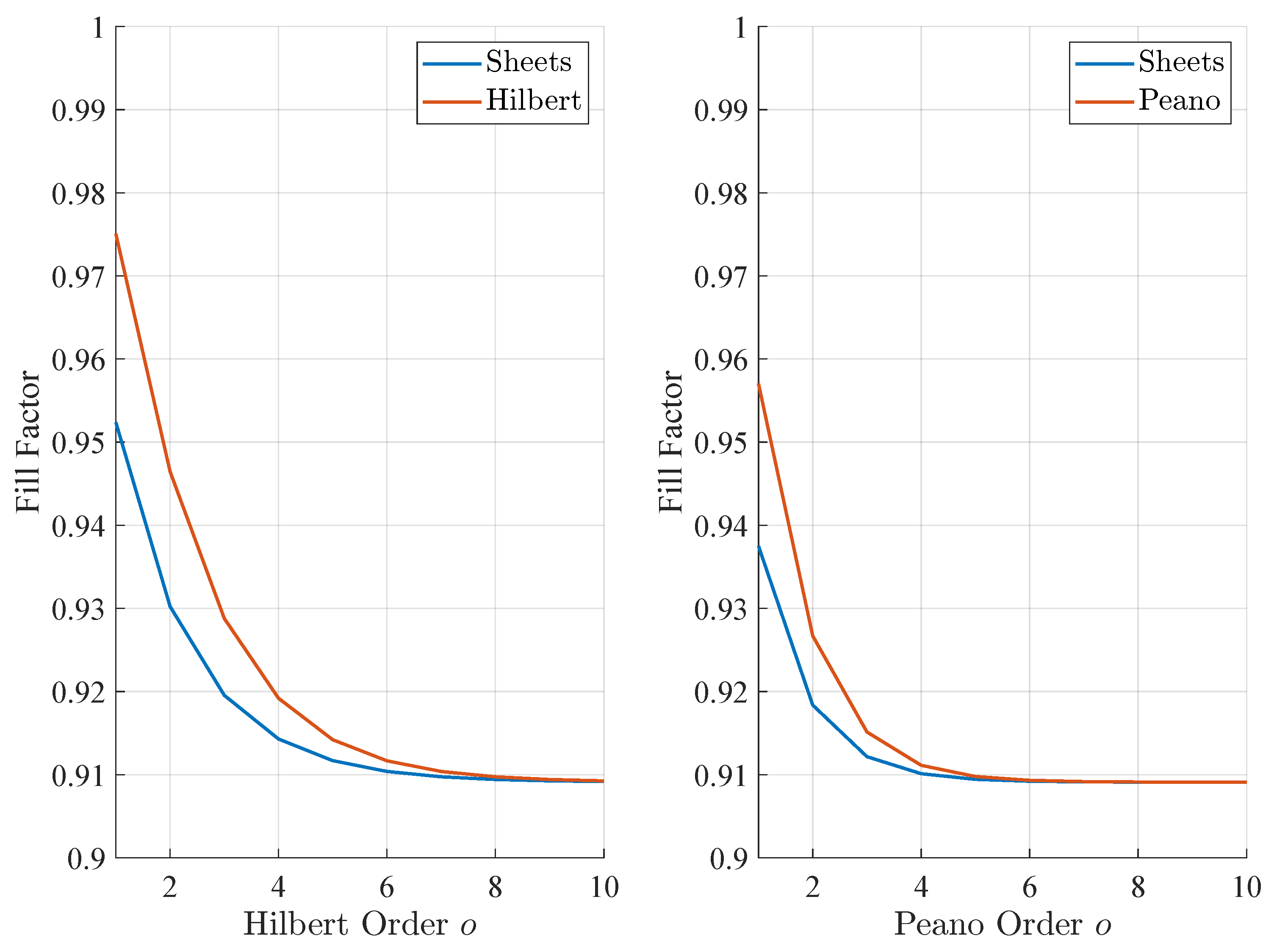
Figure 15 shows the fill factor of multiple orders of the Hilbert curve based on (28) with the respective fill factor of AM-built sheets according to (29) on the left, while the right side shows the fill factor of the Peano curve (31) which necessitates the appropriate equation for the fill factor of AM-built sheets (32). As the connection between order o and number of sheets N is different for the two SFCs, the fill factor of the AM-built sheets is not the same for both cases. As already mentioned, the AM-built sheets consistently show a lower fill factor than the SFCs. However, the difference decreases with an increasing order o and both SFCs as well as the AM-built sheets converge to a fill factor of $0.909$. This value is the fill factor of laminated sheets when inserting $w=0.5\mathrm{mm}$ and $50\mathsf{\mu }\mathrm{m}$ into (23). Another interesting fact is that the fill factor is highest for a low order o. A one-to-one comparison between the SFCs is not possible as either at least one of the widths w or $w_g$ has to be different between the SFCs or the total area filled changes. It is also clear that this comparison would be highly dependent on the order of the SFCs. However, in a real world application, the targeted area $A_{total}$ is usually given such that the maximum order is limited by the smallest manufacturable structure and gap sizes. This leads to an ideal structural width w which differs for each SFC and the respective fill factors can be calculated.

5. Conclusions

A number of soft-magnetic components based on space-filling curves (SFCs) were investigated and compared to components comprised of sheets with respect to both specific eddy current losses and fill factor. A method for estimating the eddy current loss density analytically was proposed, although an error based on the geometric parameters of the structure remains and necessitates further investigation. Sheets with a thickness equal to the nominal width of the SFC structures exhibit specific eddy current losses which are as much as $27\%$ lower than in the SFC structure. However, analysis has shown the fill factor of the SFCs to be superior compared to that of sheets when filling the same volume and while applying the same constraints concerning achievable structure and insulating gap width. Therefore, a compromise between eddy current losses and fill factor has to be made when designing novel soft-magnetic components for AM-built electrical machines.

A critical next step in this research topic is to experimentally investigate the proposed structures. This will require careful planning as the components are non-standard and some methods such as using an Epstein frame may not be feasible. Another attribute which is yet to be investigated is the mechanical stability. Depending on the orientation of the SFCs or sheets with air gaps as insulation, some mechanical loads may be favourable to others. Thus, future work will investigate this and develop concepts for improving the mechanical stability of these structures.