
Yaw Stability Control of Unmanned Emergency Supplies Transportation Vehicle Considering Two-Layer Model Predictive Control


Abstract
1. Introduction
- A two-layer control structure is adopted to decouple the dynamics between the yaw control system and the driving system. Compared with the integral control structure of yaw stability and torque distribution, the system dimension of the overall optimization strategy is reduced, the computational burden is reduced, and the computational efficiency of multi-objective optimization control with constraints is improved, which is easier to implement.
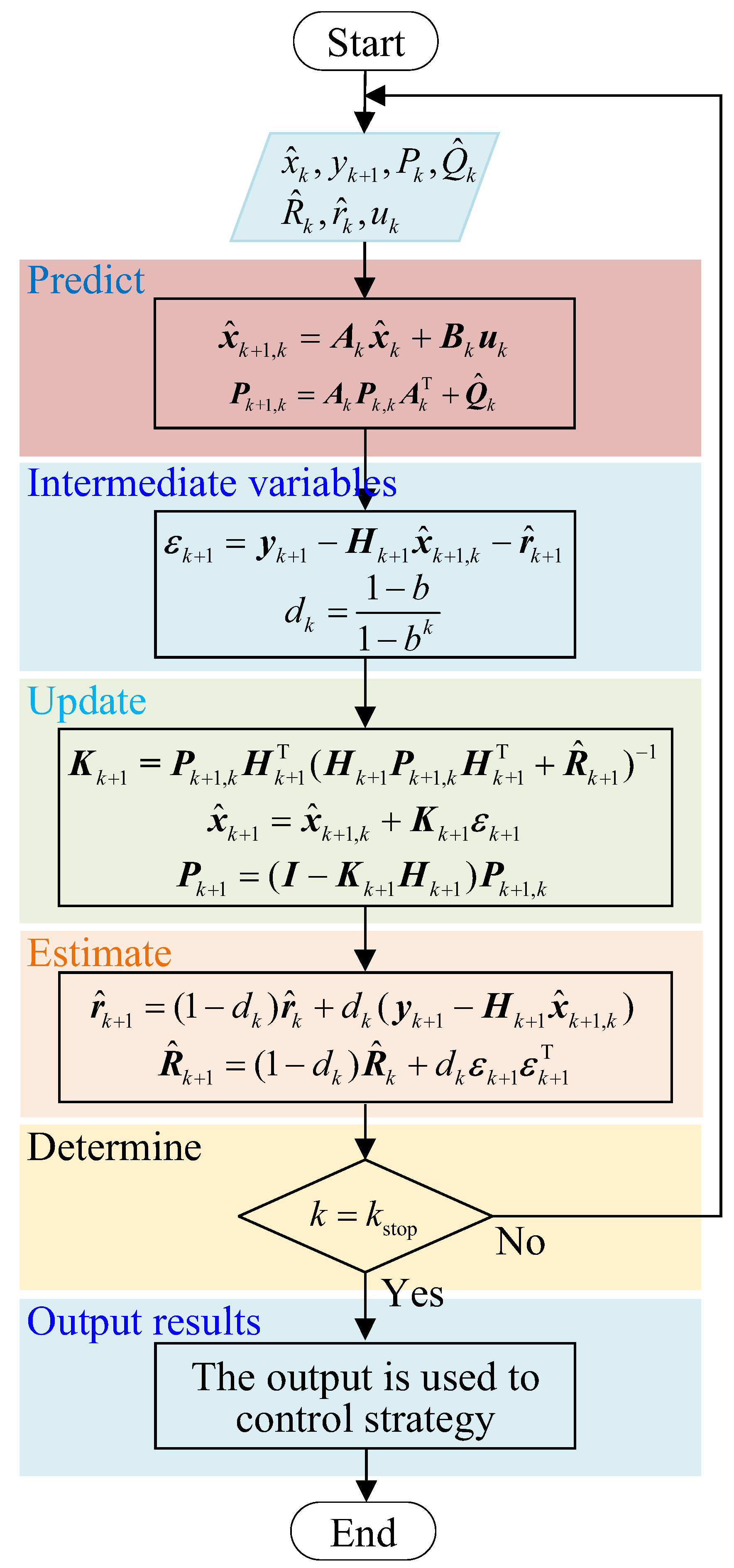
- To improve the accuracy and stability of filtering, an improved SHAEKF method that can dynamically adjust the statistical characteristics of noise in a timely manner is used to optimize the state variables, which improves the accuracy of the state variables.
- The upper-layer yaw stability controller uses MPC to solve the expected additional yaw moment and the front wheel steering angle. The lower-layer torque distribution controller uses the rolling time domain optimization method to track the additional yaw moment required for the upper-layer yaw stability.
2. Vehicle Dynamics Model
- Assume that the vehicle is operating on a flat road, and ignore the vehicle’s vertical movement.
- Assume that the suspension system and the vehicle are rigid.
- Assume that only pure lateral deflection tire characteristics are considered.
- Assume that the lateral load transfer of the wheel is not considered.
- Assume that the effect of lateral and longitudinal aerodynamics on the yaw characteristics of the vehicle is ignored.
2.1. Dynamics Model
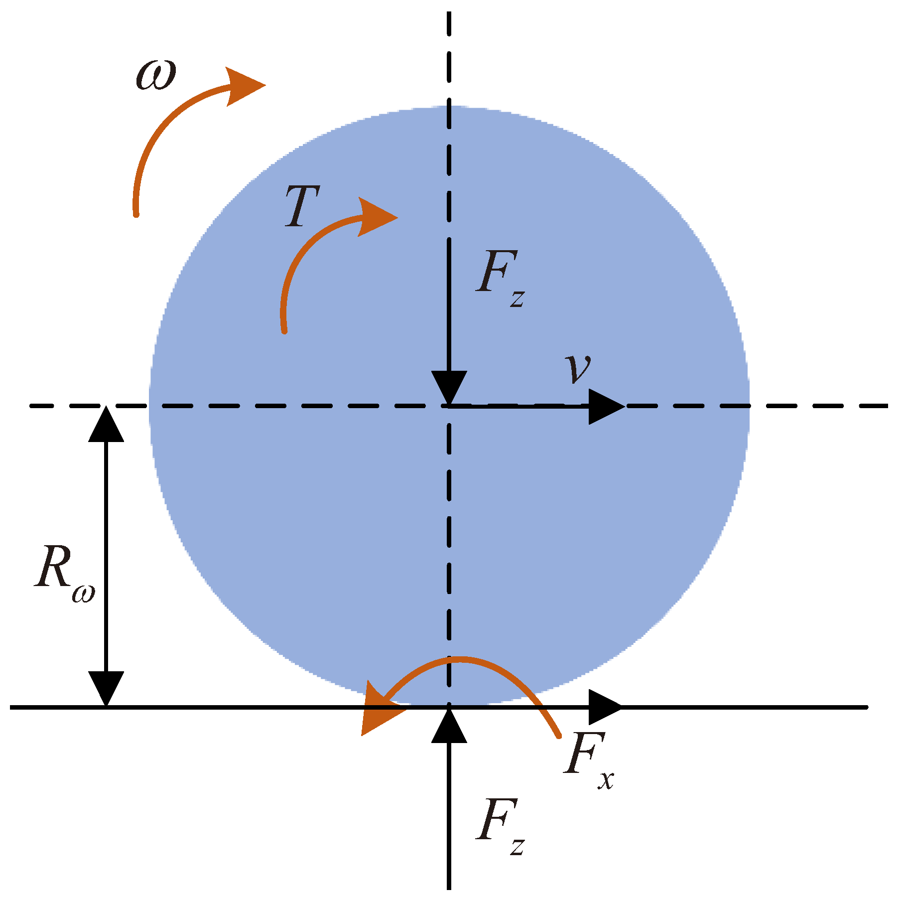
2.2. Tire Model
3. Improved SHAEKF
4. Control Strategy
5. Analysis and Validation
5.1. Simulation of Improved SHAEKF
5.2. Double Shift Trajectory Simulation
5.2.1. Comparison of Different Control Methods
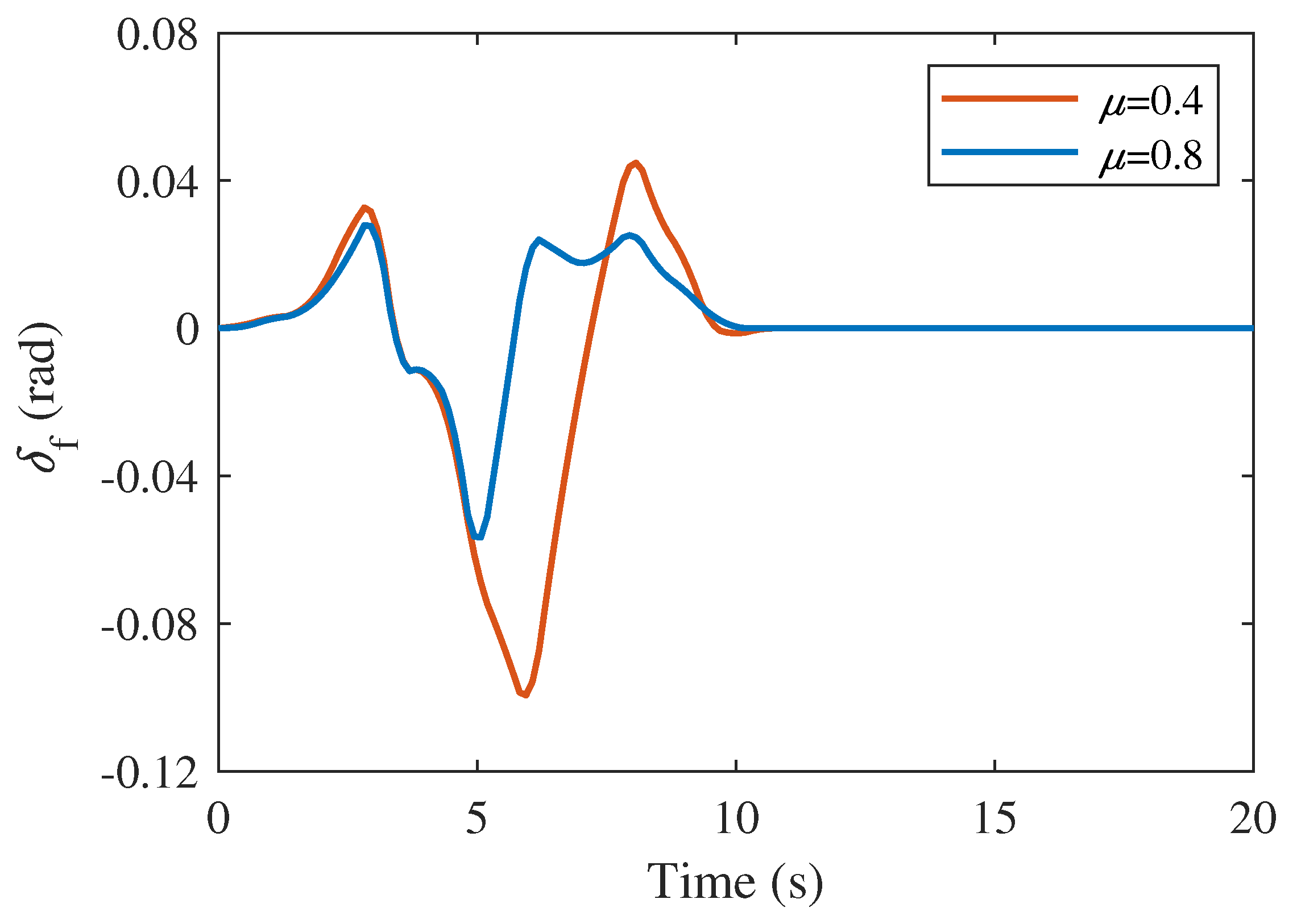
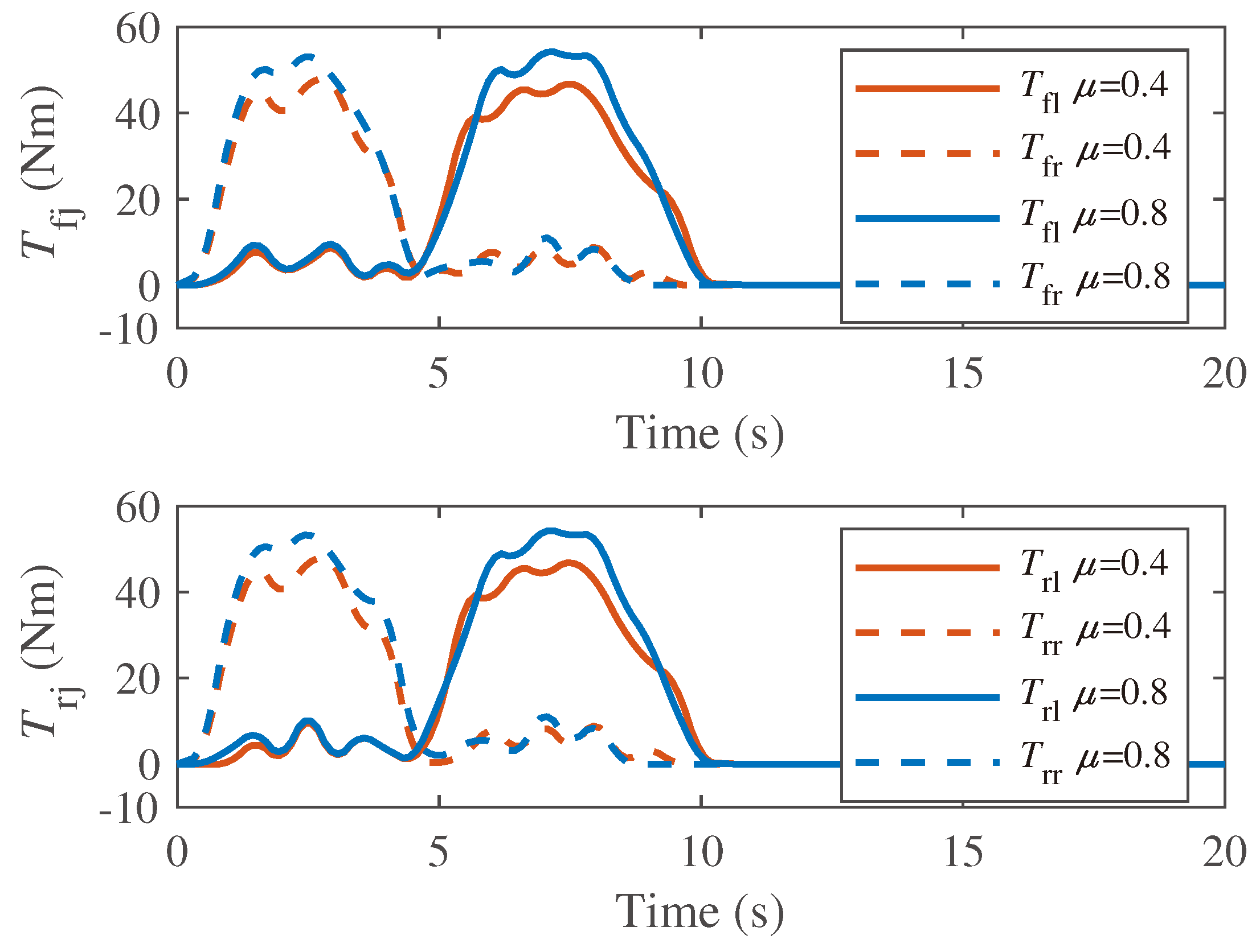
5.2.2. Robustness of the Control System to Road Adhesion Conditions
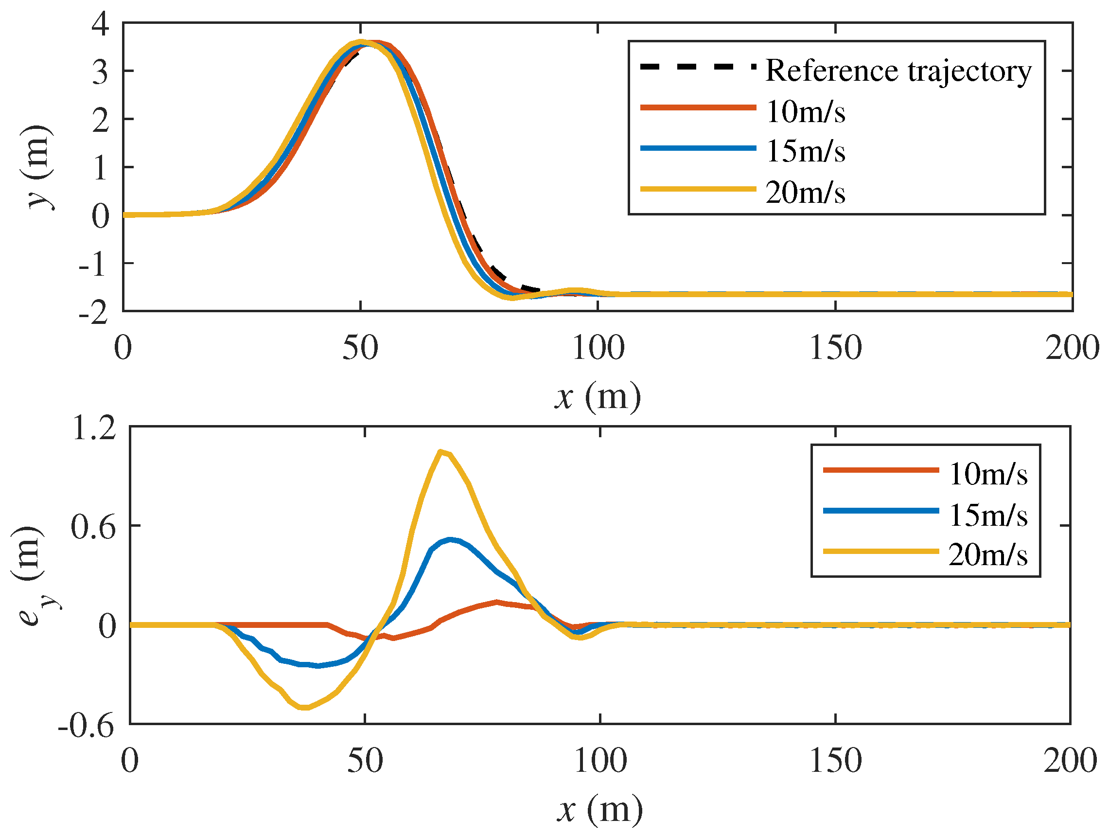
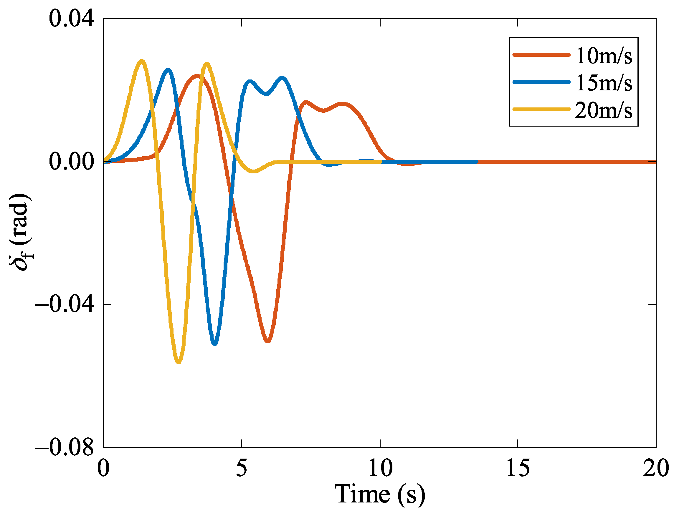
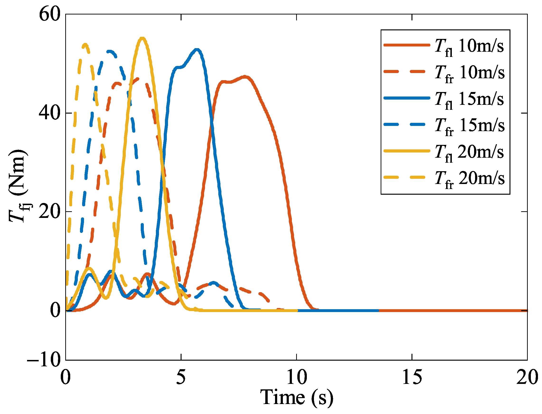
5.2.3. Robustness of the Control System to Operating Velocity
6. Conclusions
Author Contributions
Funding
Data Availability Statement
Conflicts of Interest
Abbreviations
| m | Vehicle mass |
| h | Height of center of gravity |
| d | Wheel tread |
| Distance from the center of gravity to front axle | |
| Distance from the center of gravity to rear axle | |
| Front wheel steering angle | |
| Yaw rate | |
| Sideslip angle | |
| Longitudinal and lateral velocity | |
| Longitudinal and lateral acceleration | |
| Total yaw moment | |
| Moment of inertia of vehicle | |
| Moment of inertia of wheel | |
| Wheel angular acceleration | |
| Tire rolling radius | |
| Front and rear wheel cornering stiffness | |
| Front and rear wheel longitudinal stiffness | |
| Longitudinal force of the four tires | |
| Lateral force of the four tires | |
| Drive torque |
References
- Hu, Z. A container multimodal transportation scheduling approach based on immune affinity model for emergency relief. Expert Syst. Appl. 2011, 38, 2632–2639. [Google Scholar] [CrossRef]
- Hu, X.; Yan, S.; Lin, J.; Liu, Q.; Wang, P.; Chen, H. Lateral motion control and analysis for autonomous vehicles considering road curvature. In Proceedings of the 2021 China Automation Congress, CAC 2021, Beijing, China, 22–24 October 2021. [Google Scholar]
- Li, R.; Guo, C.; Li, Y.; Zhao, Y. Trajectory tracking of intelligent vehicle based on steering and braking coordination control. Syst. Eng. Electron. 2023, 45, 1185–1192. [Google Scholar]
- Wu, X.; Wei, C.; Zhai, J.; Yuan, S. Study on the optimization of autonomous vehicle on path-following considering yaw stability. J. Mech. Eng. 2022, 58, 130–142. [Google Scholar]
- Park, M.; Yim, S. Comparative study on coordinated control of path tracking and vehicle stability for autonomous vehicles on low-friction roads. Actuators 2023, 12, 398. [Google Scholar] [CrossRef]
- Liu, L.; Zhang, L.; Pan, G.; Zhang, S. Robust yaw control of autonomous underwater vehicle based on fractional-order PID controller. Ocean Eng. 2022, 257, 111493. [Google Scholar] [CrossRef]
- Li, H.; Wang, X.; Song, S.; Li, H. Vehicle control strategies analysis based on PID and fuzzy logic control. Procedia Eng. 2016, 137, 234–243. [Google Scholar] [CrossRef]
- Patil, H.; Devika, K.B.; Vivekanandan, G.; Sivaram, S.; Subramanian, S.C. Direct yaw-moment control integrated with wheel slip regulation for heavy commercial road vehicles. IEEE Access 2022, 10, 69883–69895. [Google Scholar] [CrossRef]
- Yu, S.; Li, W.; Liu, Y.; Chen, H. Steering stability control of four-wheel-drive electric vehicle. Control Theory Appl. 2021, 38, 719–730. [Google Scholar]
- Zhou, X.; Shen, H.; Wang, Z.; Ahn, H.; Kung, Y.; Wang, J. Ground Vehicle generalized forces and moment governor design via noncertainty-equivalent adaptive prescribed performance control. In Proceedings of the 2023 IEEE International Automated Vehicle Validation Conference, IAVVC 2023, Austin, TX, USA, 16–18 October 2023. [Google Scholar]
- Hussain, N.A.A.; Ali, S.S.A.; Ovinis, M.; Arshad, M.R.; Al-Saggaf, U.M. Underactuated coupled nonlinear adaptive control synthesis using U-Model for multivariable unmanned marine robotics. IEEE Access 2020, 8, 1851–1865. [Google Scholar] [CrossRef]
- Park, B.S.; Yoo, S.J. Quantized-communication-based neural network control for formation tracking of networked multiple unmanned surface vehicles without velocity information. Eng. Appl. Artif. Intell. 2022, 114, 105160. [Google Scholar] [CrossRef]
- Taghavifar, H.; Hu, C.; Taghavifar, L.; Qin, Y.; Na, J.; Wei, C. Optimal robust control of vehicle lateral stability using damped least-square backpropagation training of neural networks. Neurocomputing 2020, 384, 256–267. [Google Scholar] [CrossRef]
- Gros, S.; Zanon, M.; Quirynen, R.; Bemporad, A.; Diehl, M. From linear to nonlinear MPC: Bridging the gap via the real-time iteration. Int. J. Control 2020, 93, 62–80. [Google Scholar] [CrossRef]
- Zhang, Z.; Xie, L.; Lu, S.; Wu, X.; Su, H. Vehicle yaw stability control with a two-layered learning MPC. Veh. Syst. Dyn. 2023, 61, 423–444. [Google Scholar] [CrossRef]
- Bossi, L.; Rottenbacher, C.; Mimmi, G.; Magni, L. Multivariable predictive control for vibrating structures: An application. Control Eng. Pract. 2011, 19, 1087–1098. [Google Scholar] [CrossRef]
- Xu, F.; Guo, Z.; Yu, S.; Chen, H.; Liu, Q. Fast realization of stability prediction controller for four-wheel drive electric vehicles. Control Theory Appl. 2022, 39, 777–787. [Google Scholar]
- Qu, Y.; Xu, F.; Yu, S.; Chen, H.; Li, Z. Model predictive control based on extended state observer for vehicle yaw stability. Control Theory Appl. 2020, 37, 941–949. [Google Scholar]
- Wang, L.; Pang, H.; Wang, P.; Liu, M.; Hu, C. A yaw stability-guaranteed hierarchical coordination control strategy for four-wheel drive electric vehicles using an unscented Kalman filter. J. Frankl. Inst. 2023, 360, 9663–9688. [Google Scholar] [CrossRef]
- Chowdhri, N.; Ferranti, L.; Iribarren, F.S.; Shyrokau, B. Integrated nonlinear model predictive control for automated driving. Control Eng. Pract. 2021, 106, 104654. [Google Scholar] [CrossRef]
- Liu, C.; Liu, H.; Han, L.; Chen, K. High-speed obstacle avoidance and stability control of distributed electric drive vehicle under extreme off-road conditions. Acta Armamentarii 2021, 42, 2102–2113. [Google Scholar]
- Zhang, C.; Feng, Y.; Wang, J.; Gao, P.; Qin, P. Vehicle sideslip angle estimation based on radial basis neural network and unscented Kalman filter algorithm. Actuators 2023, 12, 371. [Google Scholar] [CrossRef]
- Slimi, H.; Sentouh, C.; Mammar, S.; Nouveliere, L. Sensor position identification and vehicle state estimation using the extended Kalman filter. Intell. Syst. Autom. 2008, 1019, 41–46. [Google Scholar]
- You, J.; Zhang, Z.; Zhang, F.; Wu, W. Cooperative filtering and parameter identification for advection-diffusion processes using a mobile sensor network. IEEE Trans. Control Syst. Technol. 2023, 31, 527–542. [Google Scholar] [CrossRef]
- Dong, Z.; Yang, X.; Zheng, M.; Song, L.; Mao, Y. Parameter identification of unmanned marine vehicle manoeuvring model based on extended Kalman filter and support vector machine. Int. J. Adv. Robot. Syst. 2019, 16, 1–10. [Google Scholar] [CrossRef]
- Khalkhali, M.B.; Vahedian, A.; Yazdi, H.S. Situation assessment-augmented interactive Kalman filter for multi-vehicle tracking. IEEE Trans. Intell. Transp. Syst. 2022, 23, 3766–3776. [Google Scholar] [CrossRef]
- Khalkhali, M.B.; Vahedian, A.; Yazdi, H.S. Multi-target state estimation using interactive Kalman filter for multi-vehicle tracking. IEEE Trans. Intell. Transp. Syst. 2020, 21, 1131–1144. [Google Scholar] [CrossRef]
- Smieszek, M.; Dobrzanska, M. Application of Kalman filter in navigation process of automated guided vehicles. Metrol. Meas. Syst. 2015, 22, 443–454. [Google Scholar] [CrossRef][Green Version]
- Ge, L.; Zhao, Y.; Ma, F.; Guo, K. Towards longitudinal and lateral coupling control of autonomous vehicles using offset free MPC. Control Eng. Pract. 2022, 121, 105074. [Google Scholar] [CrossRef]
- Ahangarnejad, A.H.; Baslamisli, S.C. Adap-tyre: DEKF filtering for vehicle state estimation based on tyre parameter adaptation. Int. J. Veh. Des. 2016, 71, 52–74. [Google Scholar] [CrossRef]
- Cheng, C.; Cebon, D. Parameter and state estimation for articulated heavy vehicles. Veh. Syst. Dyn. 2011, 49, 399–418. [Google Scholar] [CrossRef]
- Hajiyev, C.; Soken, H.E. Robust adaptive Kalman filter for estimation of UAV dynamics in the presence of sensor/actuator faults. Aerosp. Sci. Technol. 2013, 28, 376–383. [Google Scholar] [CrossRef]
- Bahraini, M.S. On the efficiency of SLAM using adaptive unscented Kalman filter. Iran. J. Sci. Technol. Trans. Mech. Eng. 2020, 44, 727–735. [Google Scholar] [CrossRef]
- Mosconi, L.; Farroni, F.; Sakhnevych, A.; Timpone, F.; Gerbino, F. Adaptive vehicle dynamics state estimator for onboard automotive applications and performance analysis. Veh. Syst. Dyn. 2023, 61, 3244–3268. [Google Scholar] [CrossRef]
- Wang, X.; Wang, A.; Wang, D.; Xiong, Y.; Liang, B.; Qi, Y. A modified Sage-Husa adaptive Kalman filter for state estimation of electric vehicle servo control system. Energy Rep. 2022, 8, 20–27. [Google Scholar] [CrossRef]
- Ding, S.; Sun, J. Direct yaw-moment control for 4WID electric vehicle via finite-time control technique. Nonlinear Dyn. 2017, 88, 239–254. [Google Scholar] [CrossRef]
- Ren, B.; Chen, H.; Zhao, H.; Yuan, L. MPC-based yaw stability control in in-wheel-motored EV via active front steering and motor torque distribution. Mechatronics 2016, 38, 103–114. [Google Scholar] [CrossRef]
- Li, G.; Zhao, D.; Xie, R.; Han, H.; Zong, C. Vehicle state estimation based on improved Sage-Husa adaptive extended Kalman filtering. Automot. Eng. 2015, 37, 1426–1432. [Google Scholar]
- Zhang, C. Approach to adaptive filtering algorithm. Acta Aeronaut. Astronaut. Sin. 1998, S1, 97–100. [Google Scholar]
- Xu, L.; Li, S.; Qu, X. Robust adaptive algorithm for transfer alignment. J. Syst. Simul. 2012, 24, 2324–2328. [Google Scholar]
- Fnadi, M.; Du, W.; Plumet, F.; Benamar, F. Constrained model predictive control for dynamic path tracking of a bi-steerable rover on slippery grounds. Control Eng. Pract. 2021, 107, 104693. [Google Scholar] [CrossRef]


| Definition | Value |
|---|---|
| Vehicle mass m | 930 kg |
| Moment of inertia | 1372 |
| Distance from the center of gravity to front axle | 0.986 m |
| Distance from the center of gravity to rear axle | 1.253 m |
| Wheel tread d | 1.14 m |
| Tire rolling radius | 0.26 m |
| Definition | Controller Value |
|---|---|
| Predictive time domain | 15 |
| Control time domain | 5 |
| Sampling time T | 0.05 s |
| Weight coefficient matrix | |
| Weight coefficient matrix | 60 |
| Weight coefficient matrix | 100 |
| State Variables | Original Data | KF | AKF | SHAEKF |
|---|---|---|---|---|
| maximum value | 0.1659 m | 0.1249 m | 0.0968 m | 0.0847 m |
| maximum value | 0.2666 m | 0.1618 m | 0.1016 m | 0.0882 m |
| average value | 0.0038 m | 0.0027 m | 0.0017 m | 0.0013 m |
| average value | 0.0049 m | 0.0034 m | 0.0022 m | 0.0011 m |
| variance | ||||
| variance |
Disclaimer/Publisher’s Note: The statements, opinions and data contained in all publications are solely those of the individual author(s) and contributor(s) and not of MDPI and/or the editor(s). MDPI and/or the editor(s) disclaim responsibility for any injury to people or property resulting from any ideas, methods, instructions or products referred to in the content. |
© 2024 by the authors. Licensee MDPI, Basel, Switzerland. This article is an open access article distributed under the terms and conditions of the Creative Commons Attribution (CC BY) license (https://creativecommons.org/licenses/by/4.0/).
Share and Cite
Tang, M.; Zhang, Y.; Wang, W.; An, B.; Yan, Y. Yaw Stability Control of Unmanned Emergency Supplies Transportation Vehicle Considering Two-Layer Model Predictive Control. Actuators 2024, 13, 103. https://doi.org/10.3390/act13030103
Tang M, Zhang Y, Wang W, An B, Yan Y. Yaw Stability Control of Unmanned Emergency Supplies Transportation Vehicle Considering Two-Layer Model Predictive Control. Actuators. 2024; 13(3):103. https://doi.org/10.3390/act13030103
Chicago/Turabian StyleTang, Minan, Yaqi Zhang, Wenjuan Wang, Bo An, and Yaguang Yan. 2024. "Yaw Stability Control of Unmanned Emergency Supplies Transportation Vehicle Considering Two-Layer Model Predictive Control" Actuators 13, no. 3: 103. https://doi.org/10.3390/act13030103
APA StyleTang, M., Zhang, Y., Wang, W., An, B., & Yan, Y. (2024). Yaw Stability Control of Unmanned Emergency Supplies Transportation Vehicle Considering Two-Layer Model Predictive Control. Actuators, 13(3), 103. https://doi.org/10.3390/act13030103