Abstract
Because of their low cost, large workspace, and high flexibility, industrial robots have recently received significant attention in large-scale part machining. However, due to the stiffness limitations in robot joints and links, industrial robots are prone to vibration during milling processes, which leads to poor surface topography. In robotic milling processes, it remains challenging to simulate the surface topography accurately. This paper presents a mathematical model of surface topography combined with the effects of process parameters and tool vibrations in robotic milling. In this method, the kinematic trajectory of the cutting edge is first calculated by considering the cutter geometry, tool eccentricity, tool orientation, and redundancy angle. After that, the posture-dependent dynamic characteristics of the robotic milling system are predicted using an inverse distance-weighted approach. Then, a dynamic model of the robotic milling system is constructed for calculating tool vibration displacements. Finally, the kinematic model of cutting edges is modified using Z-map to incorporate the obtained vibration displacements into the sweep surfaces. In addition, milling experiments are carried out to verify the effectiveness of the proposed method, showing a good agreement between predicted and measured surface roughness. Furthermore, the findings offer valuable insights into the impact of process parameters and robot posture on surface quality.
1. Introduction
Industrial robots are becoming increasingly popular due to the advantages of low cost, high flexibility, and large workspace. Robotic milling machines, in contrast to conventional CNC (Computer Numerical Control) machines, exhibit significantly lower stiffness and heightened sensitivity to posture. The inherent characteristics of robotic milling systems make them susceptible to vibration chatter, posing substantial challenges in attaining satisfactory surface quality and machining accuracy during milling processes. Surface topography is significantly influenced by cutter runout, inclination angle, path interval, spindle speed, feed rate, and tool vibration. Surface topography plays an important role in assessing the quality of machined surface, and predicting it accurately is essential for optimizing milling processes. While conventional CNC machines have been extensively studied analytically and experimentally for surface topography prediction, there has been relatively little research focused on predicting the surface topography from robotic mill operations. The purpose of this study is, therefore, to illustrate the effect of process parameters and tool vibrations on surface topography during robotic milling.
Most early efforts focused on developing analytical methods and experiments for predicting surface topography of CNC machines in view of the influence of cutting parameters. For example, Sekineet et al. [1] developed a mathematical model for five-axis milling to investigate path-interval and feed-interval scallops on the machined surface. Based on the swept surface of the cutting edge and N-buffer model, Xu et al. [2] proposed a precise interpolation method for cusp height calculation of CNC machine tools and then investigated the impact of various cutting parameters such as spindle speed, feed rate, inclination angle, path interval, and cutter runout. Zhao et al. [3] proposed a method for predicting stochastic topography using empirical data, which investigated the effect of process parameters on stochastic topography by using regression functions to determine the relationship between process parameters (cutting depth, cutting width, feed rate). The impact of title angle on surface quality was studied by Klauer et al. [4]. Over short wavelengths, tilt angle has a critical impact on roughness and machined geometry. As mentioned above, several primary factors, such as feed rate, tool orientation, spindle speed, cutting depth, and cutting width, have been examined for their influence on surface topography, and their work has provided manufacturers with significant assistance in optimizing cutting parameters to achieve desired surface quality.
In addition to cutting parameters, many researchers have also focused on initial geometry errors. For example, Ying et al. [5] developed an equivalent fixture error model that considered datum transformation errors in machining. Denkena et al. [6] calculated flank milling surface profiles by incorporating the trajectory of the chamfer edge into the trajectory of the cutting edge. According to the study, surface generation can occur at either the cutting edge or the chamfer when using a chamfered tool. Using measured cutting tool geometry, Lavernhe et al. [7] proposed a realistic model to simulate and predict local defects of machined surfaces based upon the machining kinematics and Z-buffer model. By using modal coefficients instead of traditional roughness parameters, Li et al. [8] developed a way to measure and evaluate milled surface quality in real time, taking into account errors such as locating errors, spindle errors, and cutting tool deflections. With tool eccentricity, secondary cutting, and size effects taken into account, Zhou et al. [9] developed a mathematical model for predicting surface topography and roughness accurately in helical milling. Arizmendi and Jiménez [10] develop a method for estimating the height of the surface topography at each grid point based on discretizing the milled surface and considering the axial and radial runouts of the face mill cutters. This methodology uses Chebyshev expansions and a standard root finder to solve a polynomial equation derived from the cutting-edge trajectory equations. Due to the posture dependence of the performances, robot posture optimization can be applied to improve robot performance, which improves machining performance in turn. Bu et al. [11] optimized the robot drilling posture by employing the projection of the stiffness ellipsoid in the drilling feeding direction as an evaluation index, reducing the depth error of the countersunk hole. In order to reduce machining error, Dumas et al. [12] proposed a machining quality criterion for optimizing workpiece placement and robot kinematic redundancy. According to their research, cutting phenomena and robot stiffness can be considered for machining robots to achieve satisfactory results for finishing tasks. Using a press-and-release model and model-based reinforcement learning, Zhang et al. [13] presented a force control algorithm for robotic constant-force grinding. In this study, the feed direction had a significant impact on surface roughness in addition to robot posture. Robotic machining and CNC machining exhibit significant differences, and, as a result, process parameters that are optimized for CNC machining cannot be directly employed in robotic machining [14].
Tool vibrations are inevitable in the machining process, which adversely affects the quality of the machined surface. Slamani and Chatelain [15] employed fast Fourier transformation analysis to identify sources of error during high-speed robotic trimming, as well as to investigate how machining strategies and cutting parameters affect heat dissipation, cutting force, and path deviation. With the integration of tool vibration into the kinematic model, Chen and Wang [16] developed a surface reconstruction model using biharmonic spline interpolation. In comparison to conventional methods, the model reduces computation errors, avoids complex optimization, and is suitable for predicting free-form surfaces of workpieces. For ball-end milling, Yang et al. [17] introduced non-uniform rational B-splines (NURBS) for surface reconstruction, which improved surface topography prediction accuracy by accounting for factors such as lead angle, surface curvature, and tool vibration. Based on a cutting-edge motion model, Wang et al. [18] developed a simulation model of the vibration of the tool and thin-walled workpiece and investigated the effects of vibration on surface topography. By identifying dynamic characteristics in different milling areas, they proposed a new method for predicting texture intervals, distributions, and residual heights. Through the incorporation of the vibration displacements into the sweep surfaces of cutter cutting edges, Sun et al. [19] presented a method for predicting the surface topography during robotic machining more accurately. Due to the fact that the process parameters and robot postures are usually considered separately in many works on robotic machining, Xu et al. [20] used grey relational analysis to study the influence of these two aspects on the surface quality of the robot. It is important to realize that the work mentioned above contributes significantly to our understanding of how surfaces are generated and to the development of prediction methods. The process considers cutting parameters, cutter geometry errors, and tool vibrations. Due to posture-dependent dynamic characteristics, it is still difficult to predict surface topography accurately in robotic milling.
The purpose of this paper is to develop a more accurate model for predicting surface topography in robotic machining, taking into account the effects of the process parameters and the posture-dependent dynamic characteristics of the robotic milling system. Based on a homogeneous coordinate transformation matrix, the cutting-edge trajectory is first established by considering parameters such as cutter geometry, runout, tool orientation, redundancy angle, and cutting parameters. After that, the posture-dependent dynamic parameters of the robotic milling system are predicted using an inverse distance-weighted method based on modal tests. Based on the identified modal parameters and cutting force, a dynamic model of the robotic milling system can be developed. Using the Z-map model, the vibration displacements obtained from solving the time-periodic delay differential equation (DDE) of the robotic milling system are finally incorporated into the sweep surfaces of the cutting edges.
The remainder of this paper is organized as follows. Section 2 presents a framework for obtaining surface topography in robotic milling systems, which integrates process parameters (such as tool orientation, redundancy angle, cutter runout) with posture-dependent dynamics (tool vibration). Section 3 presents the simulation and experimental validation. Finally, the conclusions of this study are summarized in Section 4.
2. Mathematical Model of Surface Topography
The machining accuracy and surface quality in robotic milling are impacted by several factors, including link length and assembly deviations, joint kinematic errors, deformations induced by cutting forces, process parameters, and configuration-dependent dynamic characteristics of the robot. Usually, these factors are addressed through a combination of system design, calibration, and control strategies. The calibration of the kinematic parameter errors can significantly improve the absolute positioning accuracy of the industrial robot using the product of exponentials (POE) or Denavit–Hartenberg model. In order to simplify the modeling process, the following assumptions are introduced:
- Workpieces, machine tools, and fixtures are rigid, and their deformations are ignored;
- Thermal errors are not considered;
- Tool wear and system control errors are not taken into consideration;
- The fixture errors and geometrical errors of process parameters are small.
2.1. Cutting-Edge Trajectory Model
2.1.1. Coordinate System
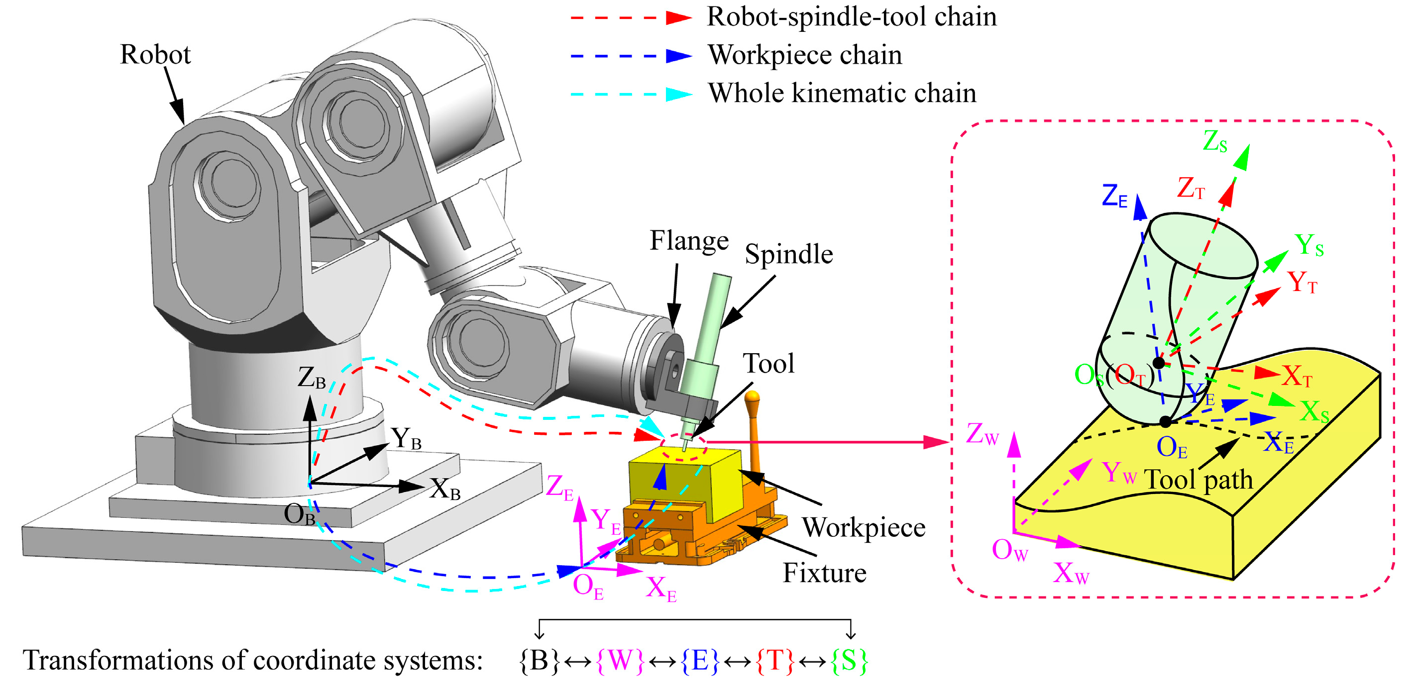
The robotic milling system is illustrated in Figure 1, which has a 6-DOF industrial robot, electric spindle, milling cutter, fixture, and workpiece. As shown in Figure 1, several coordinate systems used in modeling the sweeping surface are first introduced, as follows.
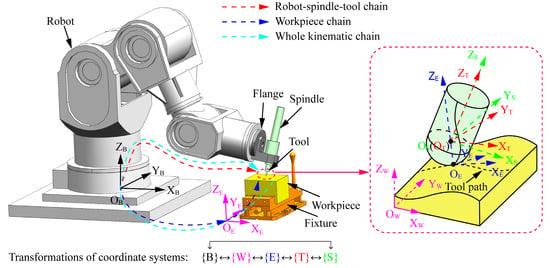
Figure 1.
Configuration of the robotic milling system coordinates.
Robot base coordinate system OB-XBYBZB, also known as {B}, is set at the center of the robot base as the global coordinate system.
Spindle coordinate system OS-XSYSZS, also known as {S}, is a local coordinate system that is fixed to the spindle. The ZS axis coincides with the spindle axis. The XS axis is along the feed direction if tilt angle and lead angle are both zero. YS can be calculated according to the right-hand rule.
Tool coordinate system OT-XTYTZT, also known as {T}, is a local coordinate system attached to the milling tool. The origin OT is defined at the tool center. The ZT axis coincides with the tool axis direction. The XT-axis is perpendicular to the tool axis and tangent to the projection of the first cutting edge. YT can be calculated according to the right-hand rule.
Workpiece coordinate system OW-XWYWZW, also known as {W}, is a local coordinate system attached to the workpiece, in which the cutter location (CL) file is described. The origin OW should be located in an easy-to-calibrate position.
Engagement coordinate system OE-XEYEZE, also known as {E}, is a local coordinate system attached to the tool path. The origin OE is located at the cutter contact (CC) point on the tool path, the XE axis is parallel to the linear feed direction, the ZE axis is the normal direction of the workpiece surface at point CC, and the YE axis is equal to the cross-product of the ZE axis and XE axis. Thus, the engagement coordinate system is also known as the feed coordinate system.
During the robotic milling process, the tool center point (TCP) moves along a specified tool path in Cartesian space. There are two motion chains in robot milling processing, as shown in Figure 1. The first is the robot motion chain, extending from the robot base coordinate system to the tool coordinate system. The second is the workpiece motion chain, originating from the robot base coordinate system to the workpiece coordinate system. To accurately describe the machined surface topography in terms of relative displacement between the cutter and the workpiece, it is necessary to transform the cutting-edge trajectory, which is initially described in the tool coordinate system, into the workpiece coordinate system. By applying these transformations along the kinematic chain, the cutting-edge trajectory can be accurately represented in the workpiece coordinate system.
2.1.2. Cutting-Edge Definition
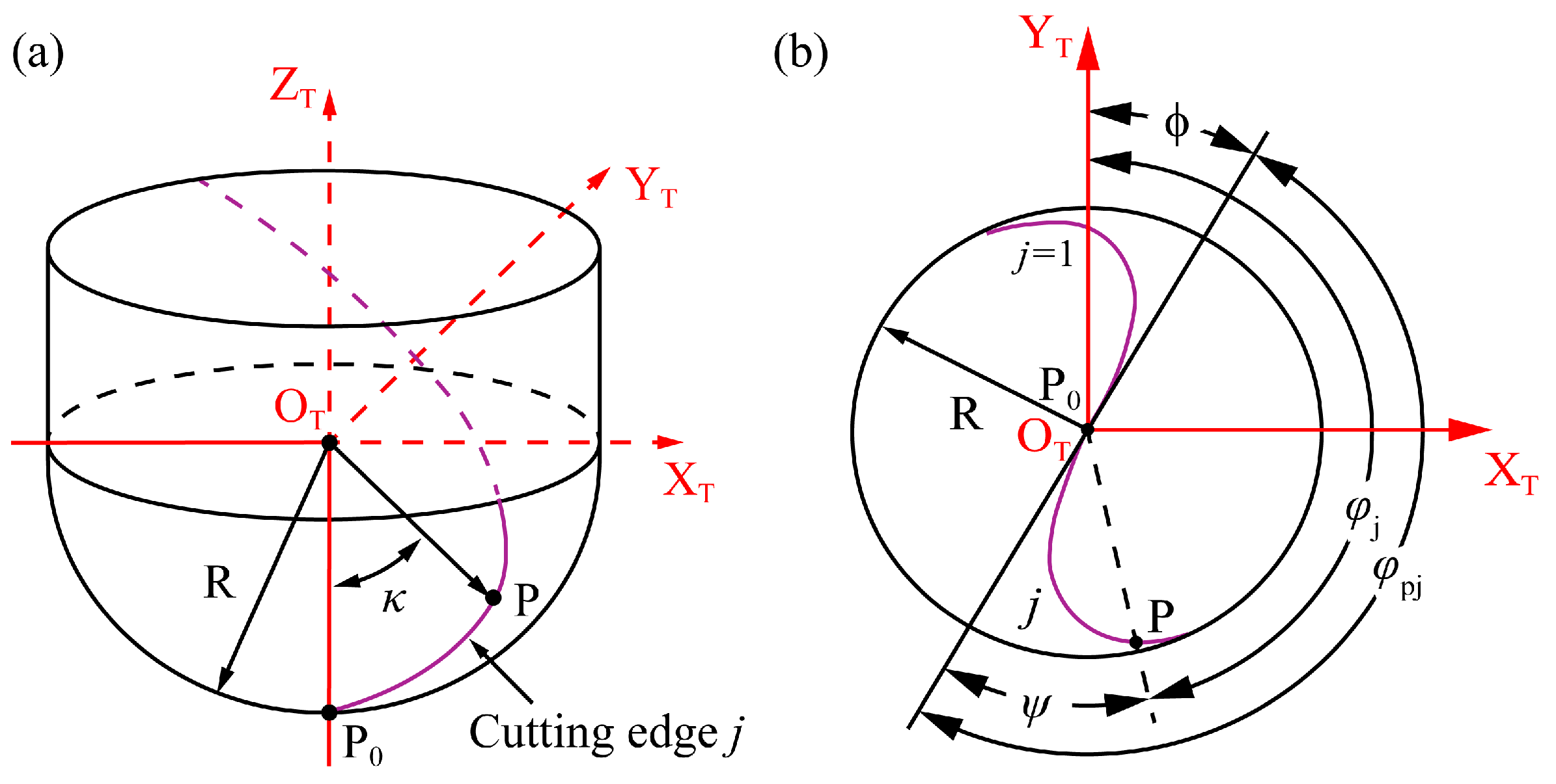
As shown in Figure 2, a ball-end milling cutter with equal pitch angle and constant lead is selected as the research object. Taking only the cutting edge on the ball end of the cutter into account, an arbitrary point P on the j-th cutter edge is
where R is the tool radius and κ is the axial position angle of the point P. The positioning angle is measured from the positive direction of YT and . is the tool rotation angle, is the pitch angle of cutting-edge j with respect to cutting edge 1, and j is the index of the cutting edge. is the lag angle of point P. These angles can be expressed as
where N is the total number of cutter teeth and is the nominal helix angle measured at the ball shank meeting boundary. The lag angle reaches its maximum value when .
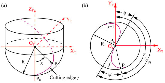
Figure 2.
(a) General view of cutting edge, and (b) Top view of cutting edge.
2.1.3. Tool Runout Definition
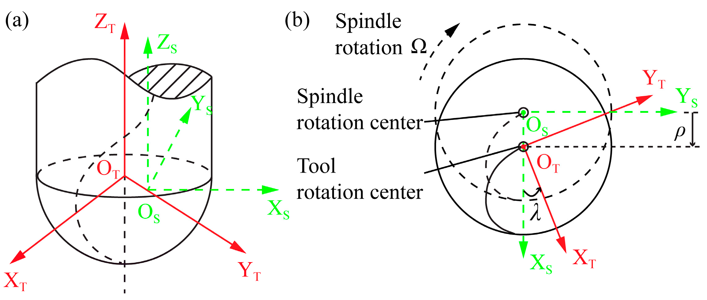
Typically, tool eccentricity occurs when the tool axis is not aligned with the spindle rotation axis, resulting in a misaligned tool movement trajectory that has a significant impact on surface morphology. Thus, it is necessary to incorporate tool eccentricity into the simulation model of surface topography. As shown in Figure 3, the cutter runout is defined by tool axis offset ρ and locating angle for offset λ. The tool coordinate system {T} rotates around the OSZS axis with angular velocity (r/min). To take the tool parallel axis offset into account, the homogeneous transformation matrix from the spindle coordinate system {S} to the tool coordinate system {T} can be expressed as
where t is the machining time along the tool path.

Figure 3.
(a) Geometry of the ball-end mill with parallel-axis runout, (b) Top view of parallel-axis runout configuration.
2.1.4. Tool Orientation Definition
Generally, a six-axis robot is used to carry out a five-axis milling operation, resulting in a redundancy degree of freedom (γ), namely rotation of the tool axis. In contrast to the redundancy angle in a machine tool, which always equals 0°, there are infinite inverse kinematic solutions to the robot inverse problem for discrete tool position points. To convert the machining trajectory defined by the workpiece coordinate system into robot end-motion trajectory, it is necessary to determine the posture of the workpiece coordinate system relative to the world coordinate system as well as the redundancy angle of the robot.
To simplify the description of the tool posture angle in machining systems, the instantaneous coordinate system as is established to describe the contact relationship between the ball-end mill and workpiece for the machined surface. The origin is located at the sphere center of the ball parts of the tool, the axis is parallel to the XE axis, the axis is parallel to the YE axis, and the axis is perpendicular to the and axes. The tool posture angle is defined as a set of tilt angles, lead angles, and redundancy angles. As shown in Figure 4, the tool coordinate system is first rotated around the Z axis of the engagement coordinate system, and this angle is defined as the redundancy angle γ. Then, the tool coordinate system rotates around the Y axis of the engagement coordinate system, and this angle is defined as the lead angle β. Finally, the tool coordinate system rotates around the X axis of the engagement coordinate system, and this angle is defined as the tilt angle α. Therefore, the tool coordinate system can be calculated by using the transformation matrix for the Z axis to the tool axial vector in the coordinate system as follows:

Figure 4.
Tool orientation transformation of the ball-end milling cutter.
2.1.5. Tool Path Definition
During robotic machining, the posture of the robot end effector (such as milling tools) is usually converted from the cutter location data CL generated by a five-axis CAD/CAM software system. They can be expressed in the workpiece coordinate system as follows:
where is the normal tool path derived from the cutter location files. The coordinate components represent the three directions along the X axis, Y axis, and Z axis, respectively. derives from the cutter axis-vector and its components and are calculated from the quaternion.
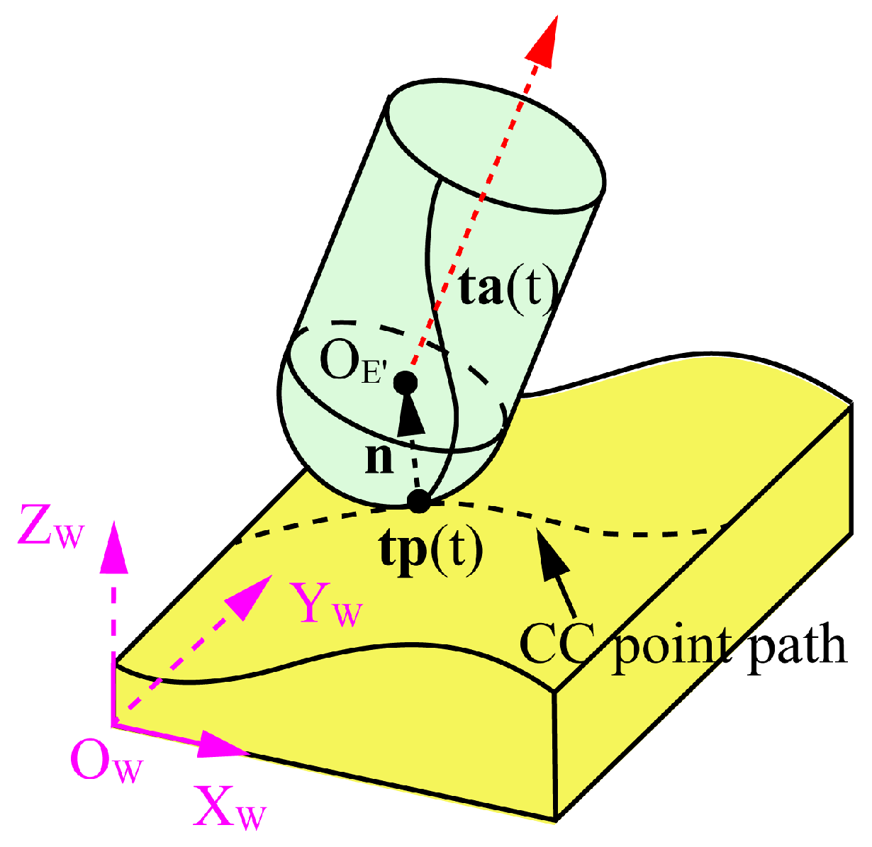
When the tool orientation is complete, the functional relation between CC point and Q(t) should be established. Figure 5 illustrates their relationship and can be expressed as the following equation:
where denotes the normal vector at the cutting contact point and represents the central point of the milling tool.
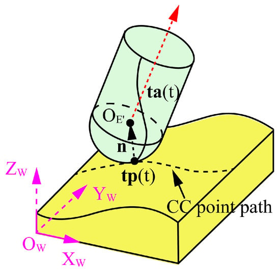
Figure 5.
Illustration of the simplified unidirectional tool path.
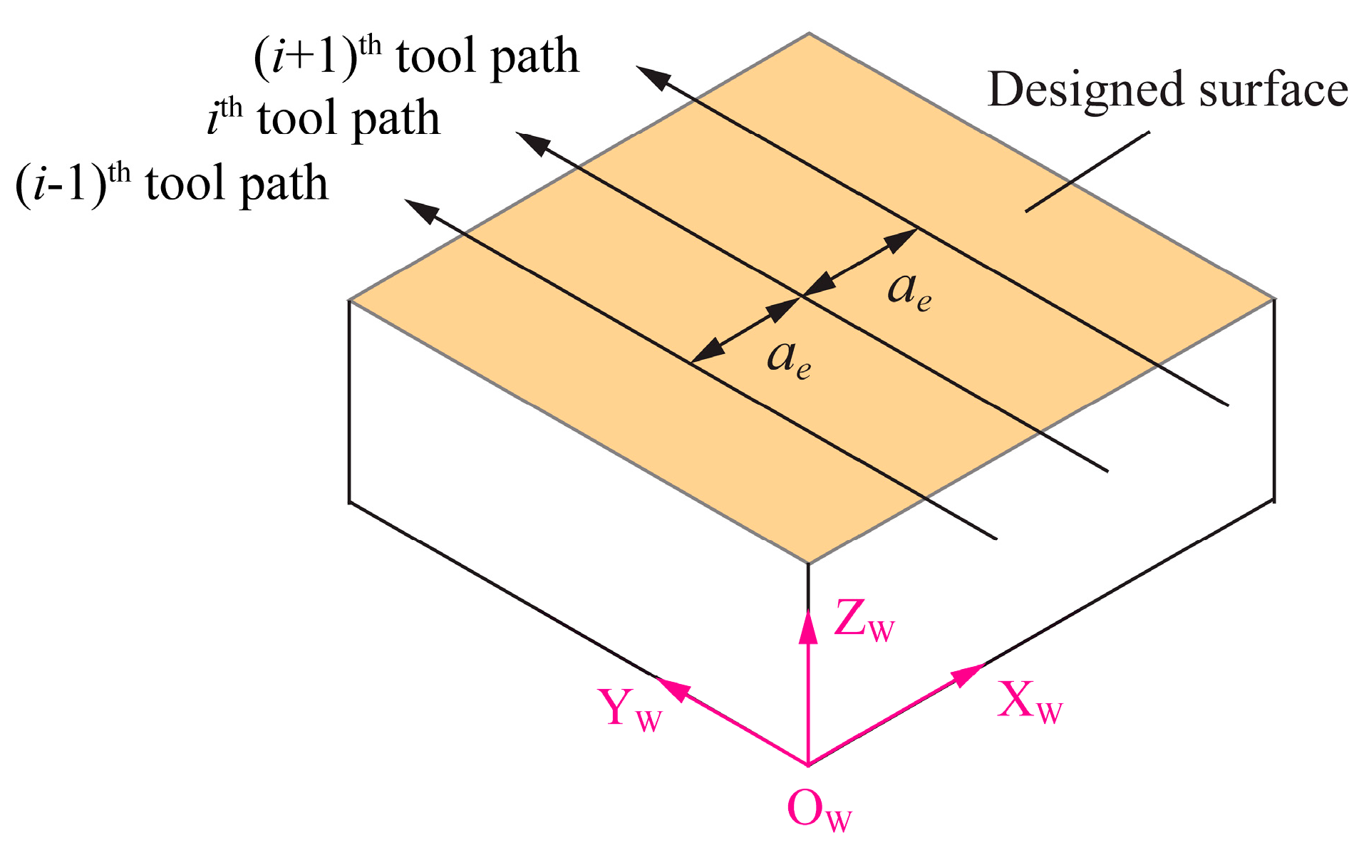
The milling cutter is presumed to move in the direction of the X axis, while the step-over between paths is directed along the Y axis. The homogeneous transformation matrix from the spindle coordinate system {E} to the tool coordinate system {W} is obtained by using the following matrix equation:
where , and are, respectively, the components of the vectors , , and in the workpiece coordinate system. , , and are the initial location of cutter contact points in the coordinate system {W}. is the feed rate (mm/s). t is the feeding time (s). is the cutting depth (mm), and is the cutting width (mm).
An example of a simplified unidirectional tool path used to carry out plane milling is shown in Figure 6. According to Equations (7) and (8), the homogeneous matrix from coordinate system to the workpiece coordinate system {W} can be rewritten as follows:
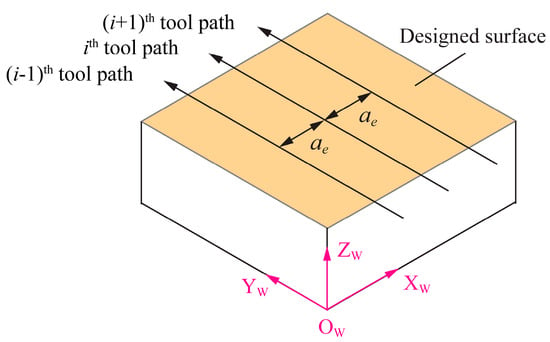
Figure 6.
Illustration of the simplified tool path.
Based on the homogeneous coordinate transformation matrix, the trajectory of the j-th cutting edge can be derived and expressed by
where the coordinates of the point P in {W} are denoted as . The position vector of the point P in {W} is represented as .
2.2. Dynamical Displacement Induced by Tool Vibration
2.2.1. Modeling of Cutting Force
Based on the cutting force model presented by Altintas [21], the cutting force components in the X axis, Y axis, and Z axis directions in the tool coordinate system {T} can be obtained from the tangential, normal, and axial force components ,, as follows:
The tangential , normal , and axial at the j-th cutting edge can be calculated using the mechanistic force model:
where ,, are the shear force coefficients, ,, are the edge force coefficients, and is the height of the cutting elements. The immersion angle of the j-th cutting edge is measured from the positive direction of YT, and . is a function used to judge whether the cutting-edge element is in cut or not. It can be defined by
where and are the entry and exit angles of the cutter j. is the instantaneous undeformed cutting thickness that has a great effect on machining force and machining stability. In robotic milling processes, robot stiffness remains constant within a short time interval, and the cutting thickness at any given moment t includes quasi-static component and dynamic components, as follows:
where is the feed per tooth, , , represent the dynamic displacement of the cutter caused by self-regeneration, and denotes the tooth passing period. The variable represents the unit normal vector of the ball-end cutter, which is expressed as follows:
2.2.2. Dynamic Model of the Robotic Milling System
In this study, the inverse distance-weighted method [22] is employed to forecast the frequency response functions (FRFs) of the tool tip, which are dependent on posture. By considering the correlation in tool tip dynamics between the unsampled points and sampled points, the FRFs at the j-th posture can be achieved by using modal data from the i-th posture in the workspace:
where is the FRFs of the j-th posture to be predicted; is the known FRFs of the i-th tested posture; and s is the number of weighted FRFs.
The joint angular distance between the predicted posture and the tested posture is used to quantify the impact of the tested posture on the predicted value. The Euclidean distance in joint space and the weight coefficients can be defined as
For a specific posture j, the predicted FRFs is defined as the ratio of harmonic displacement response at a particular node to the harmonic force at node :
where is the frequency, is the number of modes, is the modal mass of mode r, j is the imaginary unit, and are the mode shape coefficients at nodes p and q for mode r, respectively. is the pole of mode r, and * denotes complex conjugation.
The poles can be expressed as
where and are the damping ratio and eigenfrequency of mode r, respectively.
By using a partial fraction expansion, Equation (19) can be further expressed in the form of real and imaginary parts:
where the residues are composed of a modal scaling constant , and the mode shape coefficients in the two points p and q, as follows:
Equation (22) suggests that the modal scaling constant serves as a common denominator for assessing modal mass. Mode shapes are inherently arbitrarily scaled, and various methods, such as setting the largest coefficients to 1 or achieving unity length, unity modal mass, or unity modal A, can be applied [23,24]. For simplicity, this paper calculates the modal mass by scaling mode shapes to unity modal A. The modal mass, modal damping, and modal stiffness can be determined using the modalfit function in MATLAB.
Utilizing the acquired dynamic parameters and cutting force, the dynamic equations, accounting for the x, y, and z directions in the robotic milling system for a specific configuration θ in joint space, can be derived using the following equations:
where , , and are the modal mass matrix, modal damping matrix, and modal stiffness matrix, respectively. Typically, the modal matrices for robotic milling are posture-dependent, and they can be expressed as
where () are the components of modal mass, damping, and stiffness of the robotic milling system, respectively. The cutting forces represent the component forces along the X axis, Y axis, and Z axis. Additionally, represents the displacement of the cutting tool along the X axis, Y axis, and Z axis, respectively.
The dynamic displacement can be obtained from the dynamic equation using the DDE23 function in MATLAB. It is crucial to highlight that the dynamic displacements, as previously discussed, are computed in the tool coordinate system {T}. They should be further transformed into the workpiece coordinate system {W}.
2.3. Cutting Motion Correction for Vibration Displacement
In order to describe the effect of vibration on cutting motion, the vibration displacement needs to be integrated with the ideal cutting-edge trajectory. According to Equations (4) and (5), the vibration displacement of a point P on the j-th cutting edge can be expressed as a function of its coordinates in {E}, as follows:
where represent the components of the vibration displacement in the X axis, Y axis, and Z axis, respectively.
By incorporating the vibration displacement to the cutting edge trajectory of the ball-end cutter, Equation (9) can be rewritten as
Taking into account the impacts of the process parameters and vibrations of the robotic milling system, the trajectory equation of the cutting edge can be expressed as follows:
2.4. Simulation of Surface Topography
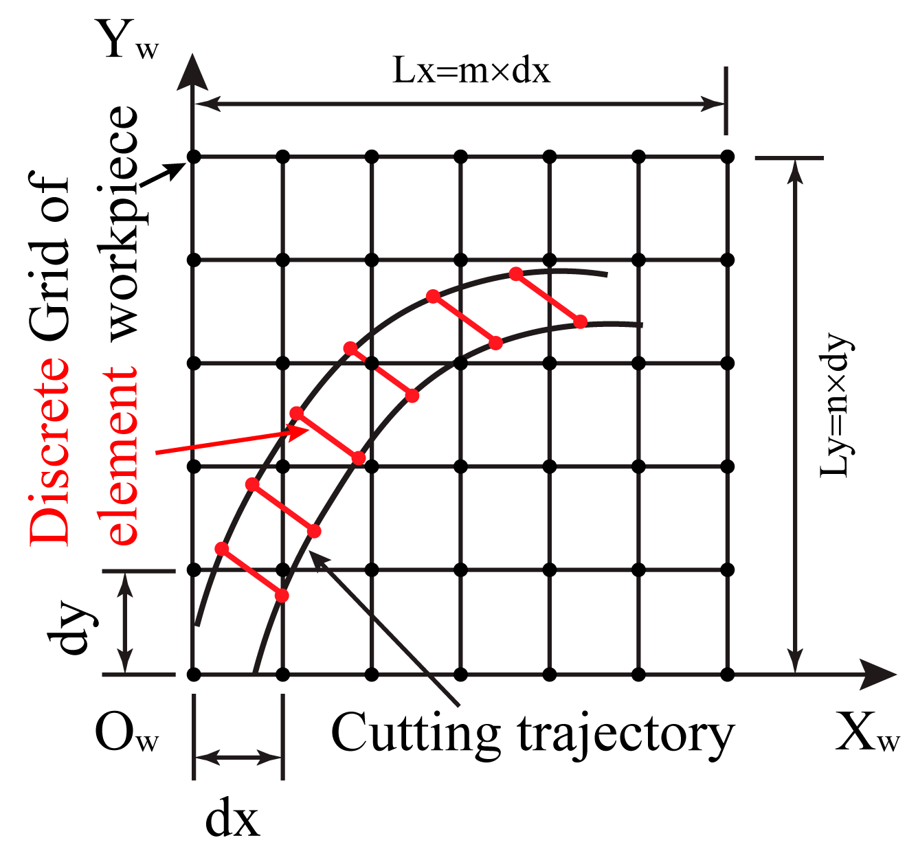
In the simulation of surface topography, the workpiece model is established using the Z-map model, employing a discretization approach. Assuming the workpiece surface is represented by , the surface is initially partitioned into grids along the X and Y directions, as illustrated in Figure 7. The coordinates of the nodes are determined by
where and represent the mesh size in the X and Y directions, respectively. In order to ensure a balance between computational accuracy and efficiency, these values are chosen according to the specific requirements of the application. Typically, the mesh size should be sufficiently small to capture fine details in the surface topography, adhering to the condition . The symbol denotes the step-over (mm). The surface topography of the workpiece is represented by the matrix , and is determined by and .
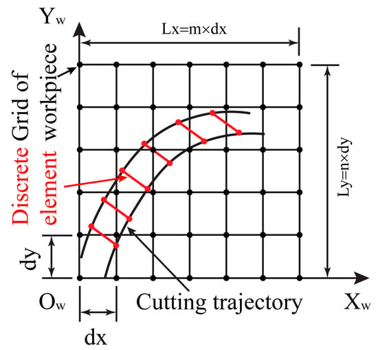
Figure 7.
Schematic of cutting trajectory projection.
The milling time is also discretized into infinitesimal elements . For each , the movement of discrete points on each cutting edge is smaller than the minimum discrete length of the workpiece. Assuming that is very small, the trajectory of discrete points on the cutting edge during this time interval is approximately linear. Therefore, the range of is determined as follows:
To ensure accuracy in the simulation, it is crucial for the discrete length of the tool to be smaller than the discrete length of the workpiece. The discrete number of points can be calculated by
where denotes the length of a discrete segment along the cutting edge.
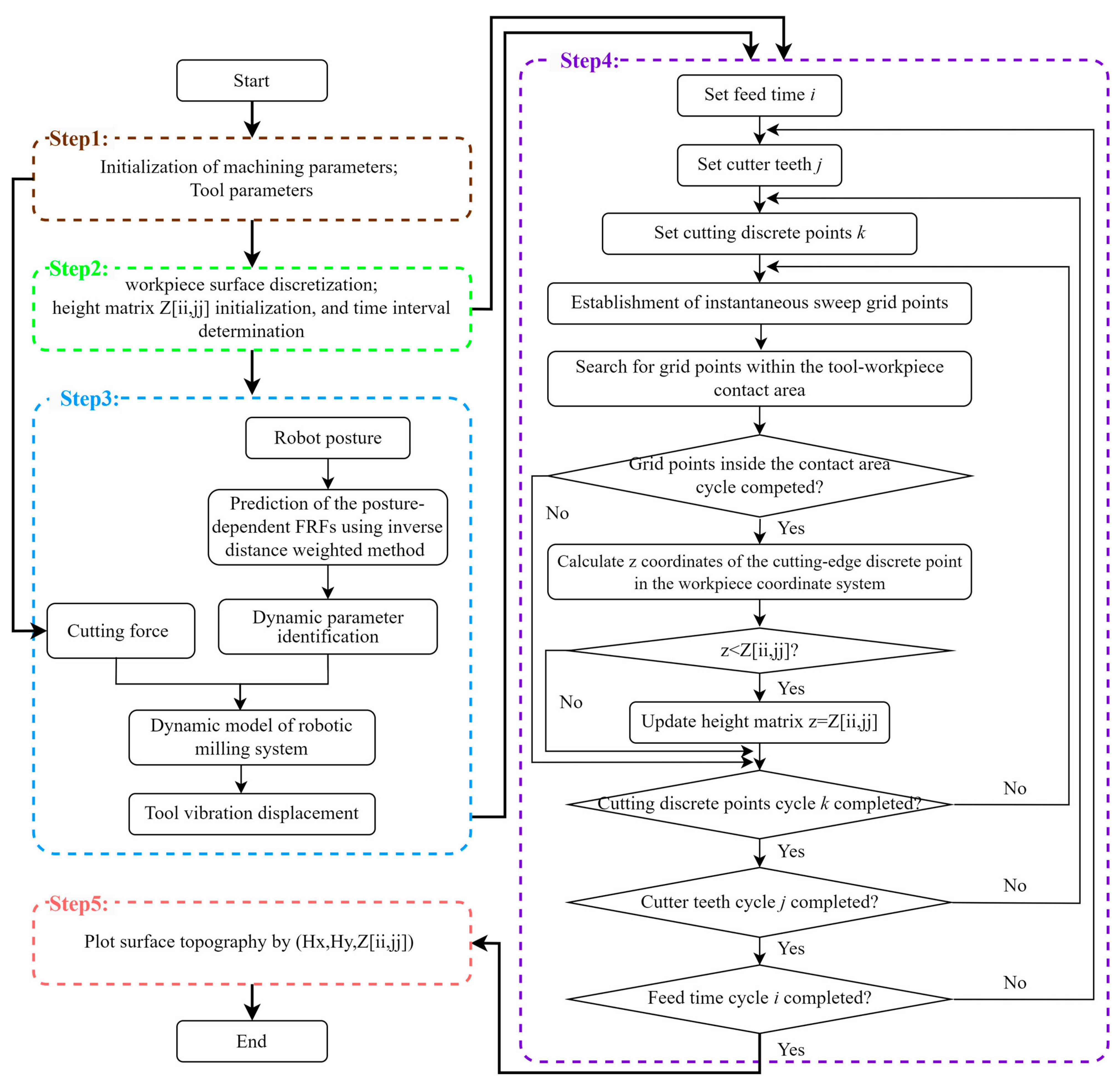
Following the surface generation mechanism of the cutting edge in robotic ball-end milling operations, the simulation of surface topography is carried out using the Z-map method. Figure 8 provides a detailed illustration of the surface topography simulation algorithm:
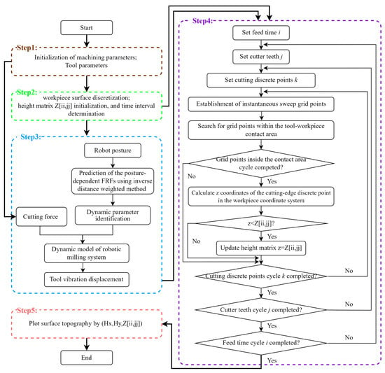
Figure 8.
Flow chart of surface topography simulation.
Step 1. Initialization: Define cutter parameters, including cutter radius, cutter runout, lead angle, tilt angle, and cutting parameters such as spindle speed, federate, depth of cut, cutting width, and redundancy angle;
Step 2: Workpiece discretization: Generate a three-dimensional grid on the workpiece surface, selecting an appropriate time step to ensure that only one grid point falls within the space covered by the cutting edge during each unit time step;
Step 3. Tool vibration displacement calculation: The total cutting forces are determined by integrating the differential force along the engaged cutting edge and subsequently summing up the contributions from all cutting edges. The FRFs at an arbitrary posture are then predicted using the inverse distance-weighted method. Subsequently, the dynamic model of the robotic milling system is constructed by incorporating the identified modal parameters and cutting force. The vibration displacement of the tool can be obtained by solving the time-periodic delay differential equation.
Step 4. Matrix Transformations: The simulation algorithm, known as Z-map, incorporates crucial components such as feed time cycle, cutter teeth cycle, and discrete cutting point cycle. During the successive cycles, the vibration displacement obtained in Step 3 is integrated into the cutting-edge equation by applying matrix transformations, resulting in the generation of a discrete point trajectory. Examine the height of every discrete point along the cutting edge, comparing it to its present value during each time interval. If the computed height is lower than the current height of the workpiece, modify the current height by incorporating the coordinate of the discrete point on the cutting edge;
Step 5. Surface topography generation: Upon completion of all iterations, update the matrix to generate a three-dimensional surface topography.
3. Experimental Verification and Analysis
3.1. Posture-Dependent Dynamic Characteristics
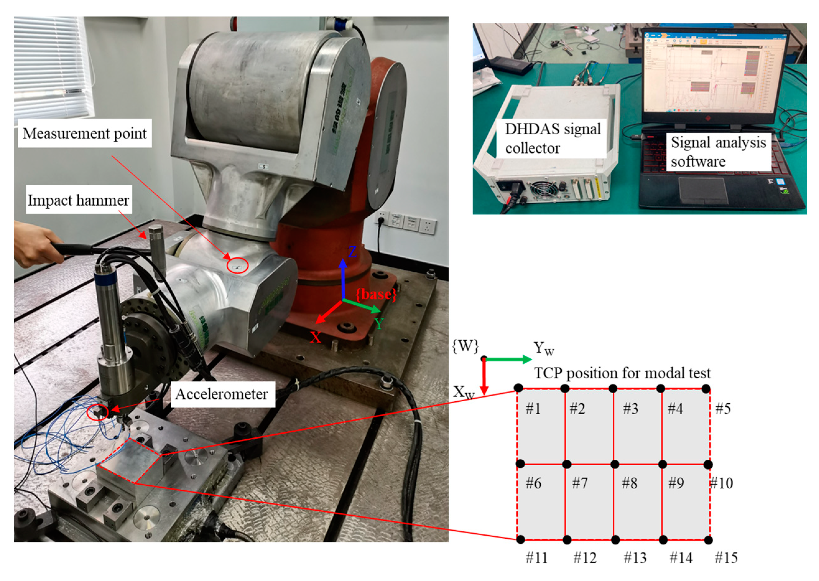
The experimental validation setup for robotic milling is illustrated in Figure 9, with a six-axis robot utilizing a Y-series harmonic reducer and equipped with a high-speed spindle attached to its end effector. An impact hammer WX-HM03 is used to excite the robot end-effector, and the acceleration responses are measured at 107 different points on the robot using a 3-axis PCB accelerometer. The input modes of the hammer and accelerometers are IEPE input mode. The excitation method used in the test is the multi-point response single-point excitation force measurement technique. FRFs are subsequently determined through the DHDAS hammer-acceleration sensor data processing system.
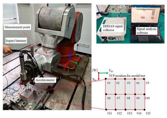
Figure 9.
Distribution of positions for impact modal tests.
In this section, 107 points on the robot body are measured using three accelerometers at each position through the group measurement method. At each specific position, five impact tests are conducted using the average method of three times of hammering. Following a consistent methodology, impact tests are carried out at 15 positions. In order to obtain the frequency response distribution characteristics of the robot under different postures, 15 TCP positions are strategically positioned within the machining plane, totaling 36 sets of impact modal tests. The chosen positions are evenly distributed across the machining plane, and Figure 9 provides a visual representation of the position distribution and numbering for clarity.
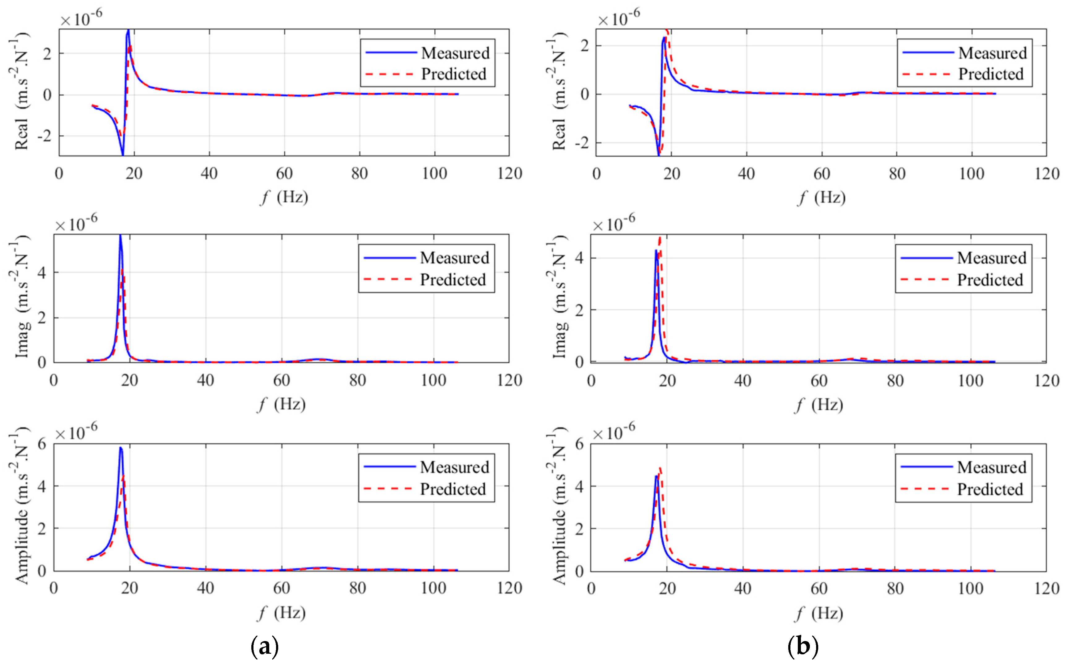
During the robotic milling process, the dominant mode of the tool tip contributes the most vibration displacement, ignoring the influence of other modes. Using the inverse distance-weighted method, a frequency response prediction for points #8 and #11 was generated based on 15 postures of experimentally acquired frequency response data. The comparison between the predicted and measured data for points #8 and #11 is depicted in Figure 10.
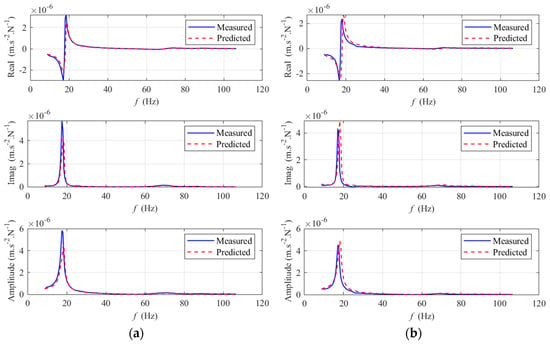
Figure 10.
Frequency response curve prediction results: (a) Posture #8, and (b) Posture #11.
Figure 10 illustrates a significant alignment between the predicted and measured frequency response results, underscoring the effectiveness of the frequency response prediction method applied in this study. The observed high level of concordance between the curves reinforces the reliability of the employed prediction approach.
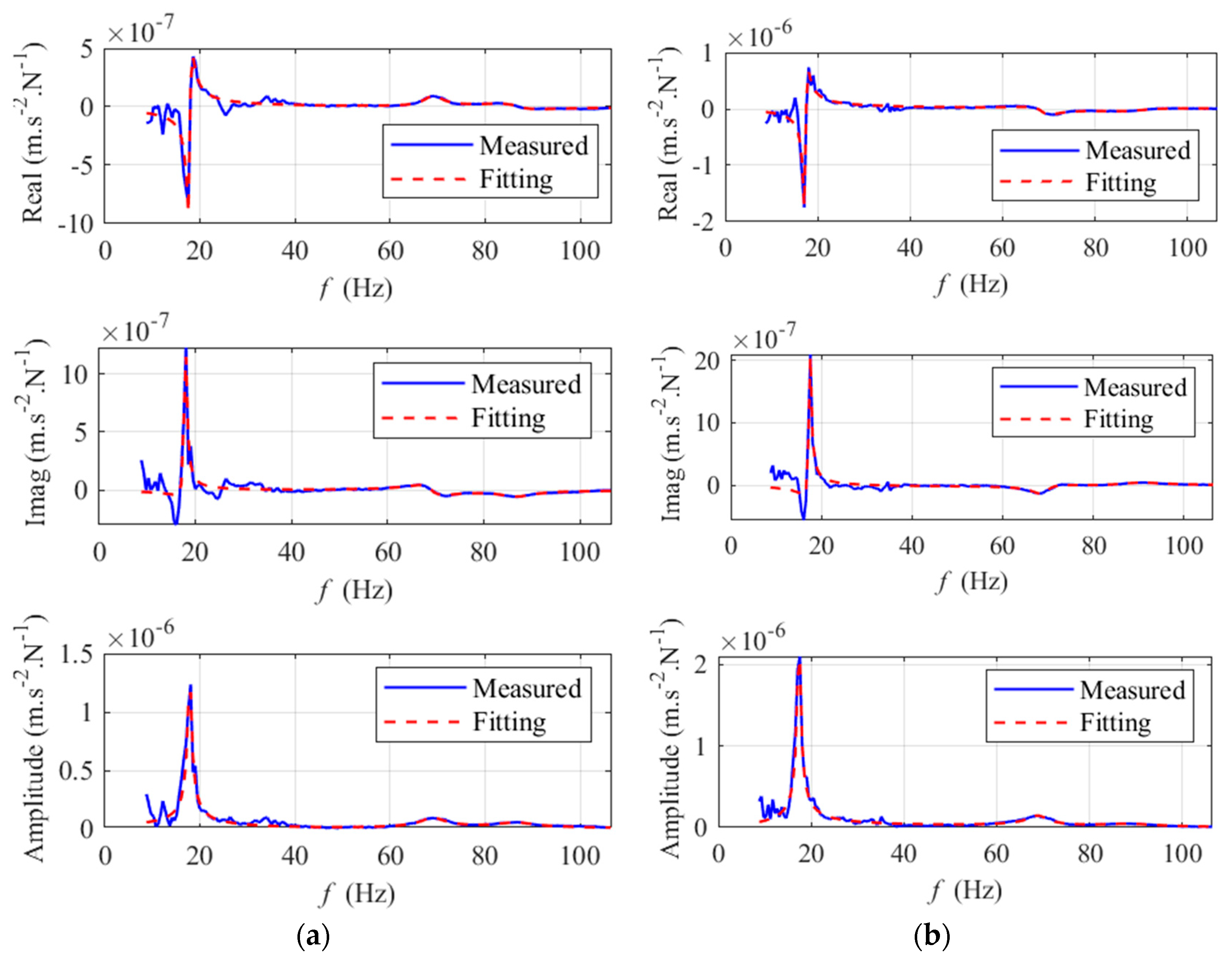
Modal parameter identification is a widely adopted approach for analyzing FRFs, serving as a crucial foundation for delving into machining vibration phenomena. As previously described, the 15 measurement positions are effectively fitted using Chebyshev orthogonal polynomials. By analyzing these fitted FRFs, the natural frequency and damping ratio for the robot processing system can be determined.
Figure 11 shows a detailed comparison of the first-order natural frequency identification at these specific points. For example, at point #8, the measured frequency is 17.54 Hz and the predicted frequency is 18.12 Hz, with a prediction error of 3.3%. Similarly, at point #11, the measured frequency is 18.36 Hz and the predicted frequency is 18.17 Hz, showing a prediction error of 1.03%. The proposed method consistently demonstrates an overall accuracy of less than 5% in predicting the modal parameters of industrial robots.
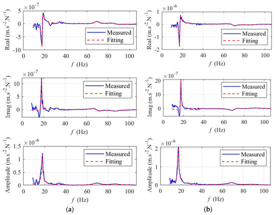
Figure 11.
Fitting frequency response curve by the orthogonal polynomials method: (a) Posture #8, and (b) Posture #11.
Significantly, the method exhibits heightened precision in predicting the positions of points located on the edges of the working plane. This highlights the effectiveness of the Chebyshev orthogonal polynomials in capturing and analyzing the modal characteristics of the robotic system. The results suggest a reliable and precise method for predicting and comprehending the dynamic behavior of the industrial robot.
3.2. Stability Analysis of Robotic Milling System
As shown in Figure 12, ball-end milling experiments were conducted on aluminum 7075-T6 workpieces with dimensions of 100 mm × 80 mm × 60 mm. Throughout these experiments, a cemented carbide mill with an 8.0 mm diameter, a helix angle of 45 degrees, and a cutter length of 25 mm was used. The cutting force signals were measured by a Kistler 9255C dynamometer, as depicted in Figure 12a. A fixture, attached to the dynamometer, securely clamped the workpiece during the experiments. A dry milling experiment was used to calculate milling force coefficients for predicting stability lobes. Subsequently, modal parameters were detected using hammer-acceleration sensor-data processing, as shown in Figure 12b. The stability lobes were predicted using the semi-discretization method [25]. Finally, cutting parameters were chosen within the stable zone for milling the material.

Figure 12.
(a) Cutting forces and chatter detection system, (b) modal parameters.
The cutting force coefficient was identified through a slot milling experiment. In this experiment, the feed per tooth was systematically varied with a fixed increment at = 0.02, 0.04, 0.06, 0.08, and 0.10 mm/tooth. The milling forces in the X axis, Y axis, and Z axis were measured using the Kistler 9255C dynamometer. Subsequently, the average milling force model was employed to identify the cutting force coefficient. According to the identification method of cutting force coefficients [26], the estimates of force coefficients are listed in Table 1.

Table 1.
Cutting force coefficients.
In the robotic milling process, the redundancy angle remained constant and did not vary. Modal parameters merely changed on the upper surface due to the small size of the experimental workpiece. To analysis the stability of the linear milling, reference point #2 was selected in the feeding direction, and its position is shown in Figure 8. The dynamic parameters of the milling system were determined by combining the inverse distance-weighted method with impact-acceleration response tests. Additionally, an accelerometer captured the vibration signal, and a Fourier transform was applied to obtain the frequency spectrogram. This spectrogram aids in determining the occurrence of chatter during the machining process. Chatter can be identified by examining the spectrogram for an increase in amplitude associated with the main mode, commonly referred to as the flutter frequency.
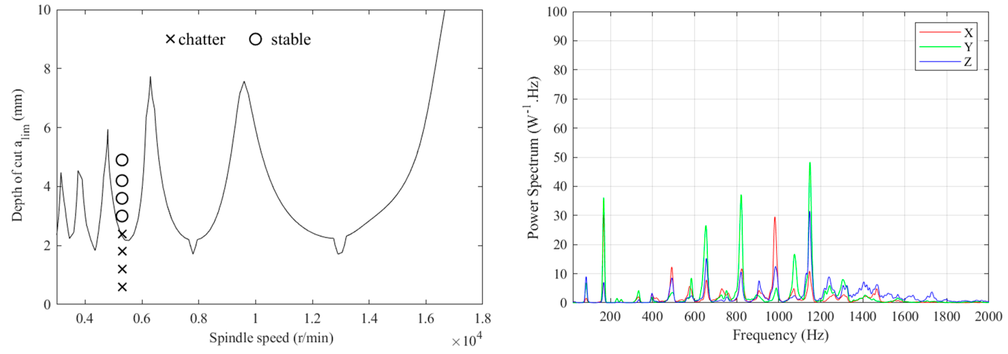
As shown in Figure 13, a semi-discretization method was used to predict stability lobes based on modal parameters. Subsequently, cutting experiments were carried out at spindle speed 5000 r/min to validate the predicted stability lobes. In the figure, ‘o’ denotes stability in the milling process with these parameters, while ‘x’ signifies destabilization. Given the use of a two-tooth cutting tool in the experiment, the cutter passing frequency was approximately 166.7 Hz at a spindle speed of 5000 r/min.
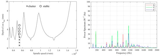
Figure 13.
Stability lobe diagram of the milling process with the selected point #2.
During the experiment with a milling depth of 1.0 mm, the dominant frequencies in the X, Y, and Z directions were primarily the harmonic frequencies of the spindle frequency (83.3 Hz). No unusual sounds occurred, and the spectrum diagram indicates the absence of other frequencies with rising amplitude, except for the larger amplitude at the conversion frequency. Consequently, the experimental results aligned with theoretical calculations, confirming stable machining conditions.
This consistency between experimental and theoretical results validates the accuracy of the proposed method for predicting stability lobes. The method is used to select machining parameters in the next section.
3.3. The Effect of Vibration on Surface Topography
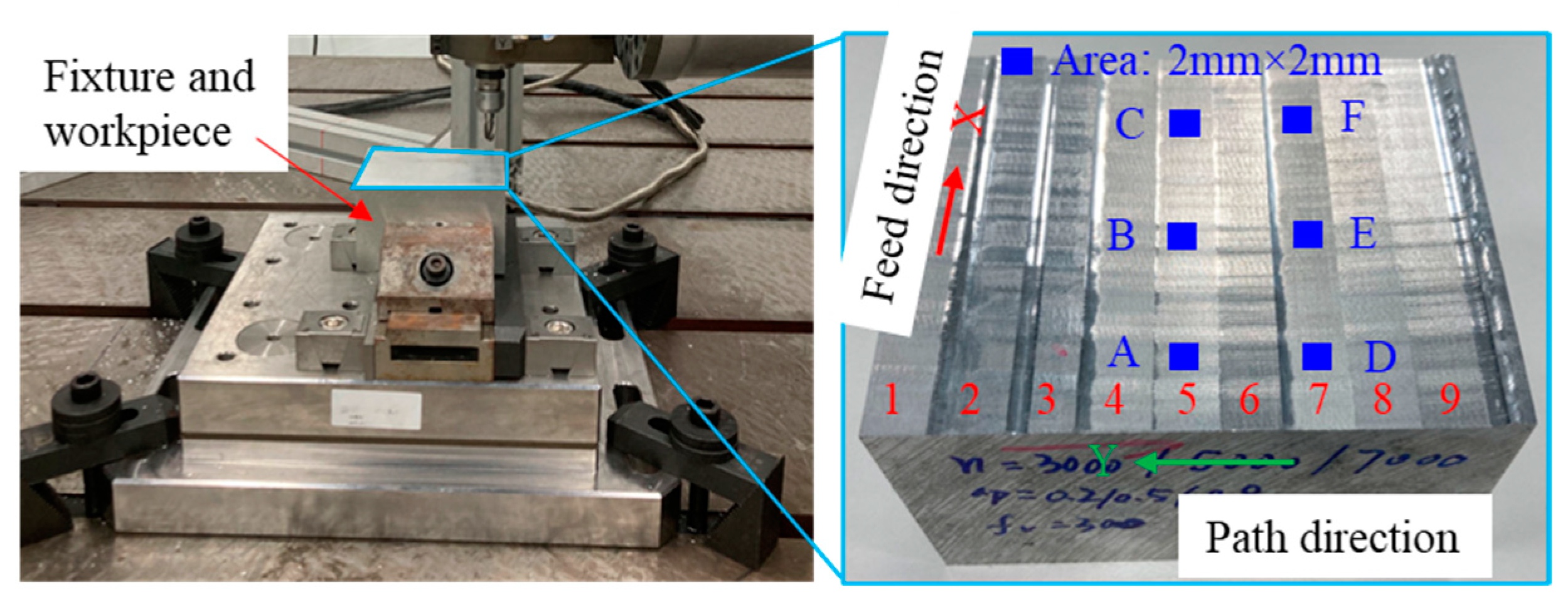
The milling experiments were carried out with a specially designed six-axis robot, employing dry milling operations. Table 2 presents an optimization of cutting parameters based on stability analysis. The machined surface of the workpiece is divided into nine zones, as illustrated in Figure 14, spanning from case 1 to case 9. For cases 5 and 7, three smaller regions (denoted as A, B, C for case 5, and D, E, F for case 7, respectively) are selected to compare simulation and experimental data on surface topography. The milling operation is carried out along the X axis, with the path direction following the Y axis. The dial gauge, illustrated in Figure 15a, is employed for tool run-out measurement. The axial runout is recorded at 0.005 mm, while the radial runout measures 0.02 mm. An Alicona optical 3D measuring instrument, as shown in Figure 15b, provides high-resolution measurements of the machined surface topography using non-contact optical methods.

Table 2.
Cutting parameters selected in the experiment.
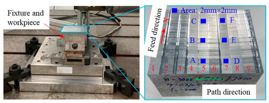
Figure 14.
Experimental results of machined surface.

Figure 15.
(a) Runout measurement using a dial gauge, (b) Optical surface roughness measurement instrument.
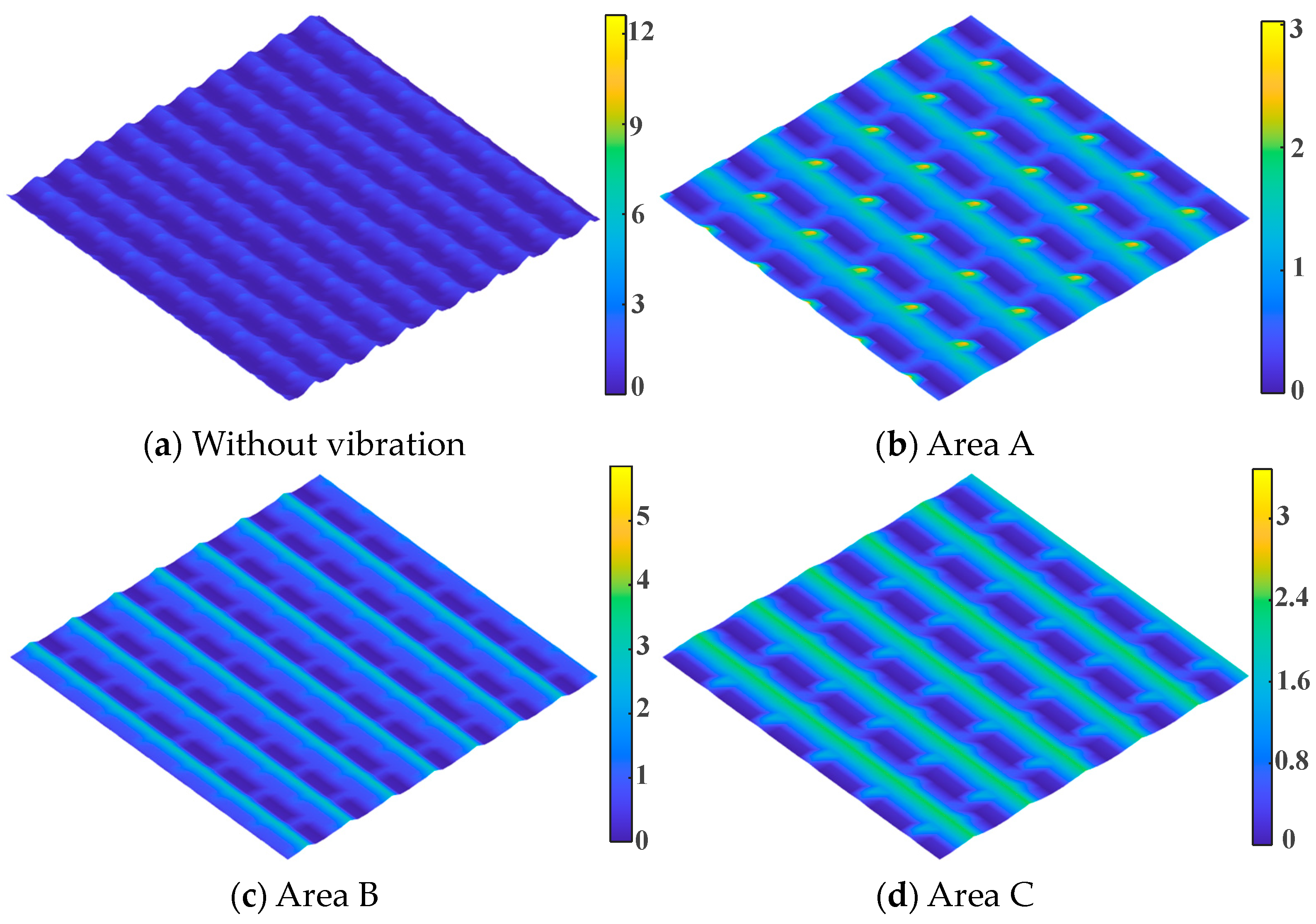
Surface topography simulations for Cases 5 and 7 (shown in Figure 14) are conducted considering both vibration and non-vibration, as illustrated in Figure 16 and Figure 17. The simulation process incorporates various parameters influencing surface generation, including spindle speed, feed rate per tooth, path interval, cutting depth, redundancy angle, and dynamic parameters related to the robotic milling system (such as stiffness, mass, and damping ratio).

Figure 16.
Simulation of surface generation model for Case 5. (a) Simulation of surface topography without considering vibration, (b) Simulation of surface topography considering vibration for Area A, (c) Simulation of surface topography considering vibration for Area B, (d) Simulation of surface topography considering vibration for Area C (unit: µm).
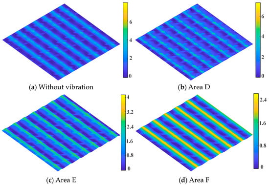
Figure 17.
Simulation of surface generation model for Case 7. (a) Simulation of surface topography without considering vibration, (b) Simulation of surface topography considering vibration for Area D, (c) Simulation of surface topography considering vibration for Area E, (d) Simulation of surface topography considering vibration for Area F (unit: µm).
During the simulation, each area (A-F, referenced in Figure 13) is defined with dimensions of 2 mm × 2 mm, utilizing a grid size of 100 × 100. MATLAB R2023B is used as the simulation platform. The choice of a 2 mm × 2 mm analysis area aligns with the measurement area outlined in Figure 14, ensuring a detailed and high-resolution representation for a specific region.
As shown in Figure 16a and Figure 17a, vibration-free machining surfaces show a relatively uniform and regular 3D contour and surface topography is arranged periodically along the path direction. Along the feed direction, the texture interval closely aligns with the feed rate per tooth, while, along the path direction, it corresponds approximately to the path interval. The residual height of the surface is relatively low.
Contrastingly, in Figure 16b–d and Figure 17b–d, it is evident that, under the influence of cutting vibration, contour fluctuation intensifies, the residual height increases, periodicity diminishes, and irregular components become more pronounced. In the feed direction, the texture interval is roughly four times larger compared to the scenario without tool vibration. Additionally, the results emphasize that, due to the posture-dependent dynamic characteristics, the residual height of the machined surface tends to increase in the direction away from the robot base system (from A to C and D to F) under identical machining parameters. These vibrations have the potential to induce tool chatter, leading to compromised surface finish and dimensional inaccuracies.
The presented analysis in Table 3 focuses on Ra (average roughness) and Rq (root mean square roughness) values obtained from simulation results with vibration across various cases (A, B, C, D, E, F). The relative error (%) is then calculated to assess the agreement between experimental and simulated results.

Table 3.
Comparison of predictions and experiments (unit: µm).
Case A reveals that both Ra and Rq exhibit relatively low relative errors, indicating a good agreement between experimental and simulated values. Compared to Case A, Case B shows relatively low errors. However, the overall error for Rq in the vibration condition is slightly higher. In contrast, Case C exhibits a higher relative error in Rq with vibration, which indicates a more pronounced deviation from experimental values.
There is a noticeable increase in Rq when vibration is introduced to Case D, although it generally displays low relative errors. In Case E, relative errors are small, but Rq increases under vibrational conditions. As in Case E, Case F exhibits small relative errors and a noticeable increase in Rq with vibration.
There is a consistent trend across the cases that indicates an increase in relative error with vibration. As a result of this trend, it seems that simulating under vibrational conditions can present some challenges. As a result, Cases C and D have higher relative errors, which highlights the difficulty in accurately simulating the experimental conditions. Results provide insightful information on how the simulation method performs under a variety of different conditions and cases.
4. Conclusions
In this paper, we develop a model to predict machined surface topography during robotic ball-end milling operations, taking various factors into account, such as tool runout, tool orientation, spindle speed, cutting depth, redundancy angle, and tool vibration. Based on this study, the key findings and conclusions can be summarized as follows:
- (1)
- The inverse distance-weighted method is particularly useful when data points are unevenly distributed across the postures of interest, providing a more accurate estimate based on proximity to the target posture;
- (2)
- The analysis shows thatthe postures of the robotic system play an important role and have a more significant impact than process parameters on milling surface quality. Therefore, milling operations should consider and optimize robot poses;
- (3)
- The combination of process parameters and robot poses estimated using the Z-map method is crucial in milling operations. Results show good agreement between predicted and measured residual heights on machined surfaces. This study provides valuable insight into the optimization of robotic milling processes for achieving desired surface quality and tolerances.
Author Contributions
J.L.: conceptualization, methodology, investigation, writing—original draft preparation. Y.N.: validation, visualization, writing—review and editing. Y.Z. (Yiyang Zhao): validation, visualization, writing—review and editing. L.Z.: supervision, conceptualization, resources, writing—review and editing. Y.Z. (Yanzheng Zhao): supervision, conceptualization, resources, writing—review and editing. All authors have read and agreed to the published version of the manuscript.
Funding
This research was funded by China Postdoctoral Science Foundation, grant number 2023M742265, and the National Key Research and Development Program of China for Robotics Serialized Harmonic Reducer Fatigue Performance Analysis and Prediction and Life Enhancement Technology Research, Grant No. 2017YFB1300603.
Data Availability Statement
All data generated or analyzed during this study are included in this paper or are available from the corresponding authors on reasonable request. Some data are not publicly available due to intellectual property protection.
Conflicts of Interest
The authors declare no conflicts of interest.
Nomenclature
| cutter radius | |
| axial position angle of the point P | |
| positioning angle from the positive direction of YT | |
| initial rotation angle | |
| pitch angle of cutting-edge j | |
| lag angle of the point P | |
| number of cutter teeth | |
| feed rate | |
| radial depth of cut | |
| axial depth of cut | |
| tool discretization disc height | |
| feed per tooth | |
| ,, | tilt angle, lead angle, redundancy angle |
| , | cutter entry and exit angle |
| instantaneous undeformed cutting thickness | |
| ,, | shear force coefficients in x/y/z direction |
| ,, | edge force coefficients in x/y/z direction |
| cutting force components in x/y/z direction | |
| vibration displacement in the x/y/z direction | |
| homogeneous transformation matrix from {S} to {T} | |
| homogeneous transformation matrix from {E} to {S} | |
| homogeneous transformation matrix from {W} to {E} | |
| frequency response function of posture | |
| frequency response function of posture | |
| number of modes | |
| spindle speed in r/min | |
| frequency in rad/s | |
| ,, | pole, damping ratio, natural frequency of mode r |
| residues | |
| mode shape coefficients of points p and q for mode r | |
| system mass, damping, and stiffness matrices |
References
- Sekine, T.; Obikawa, T.; Hoshino, M. Establishing a Novel Model for 5-Axis Milling with a Filleted End Mill. J. Adv. Mech. Des. Syst. Manuf. 2012, 6, 296–309. [Google Scholar] [CrossRef][Green Version]
- Xu, J.T.; Zhang, H.; Sun, Y.W. Swept Surface-Based Approach to Simulating Surface Topography in Ball-End CNC Milling. Int. J. Adv. Manuf. Technol. 2018, 98, 107–118. [Google Scholar] [CrossRef]
- Zhao, K.M.; Hockauf, R.; Liu, Z.B.; Zhao, W.X.; Wang, X.B.; Wang, D.Q. Kinematic and Stochastic Surface Topography of Workpiece Made of Al7075 in Flank Milling. Int. J. Adv. Manuf. Technol. 2018, 96, 2735–2745. [Google Scholar] [CrossRef]
- Klauer, K.; Eifler, M.; Kirsch, B.; Seewig, J.; Aurich, J.C. Ball End Micro Milling of Areal Material Measures: Influence of the Tilt Angle on the Resulting Surface Topography. Prod. Eng. Res. Devel. 2020, 14, 239–252. [Google Scholar] [CrossRef]
- Yang, F.; Xing, Y.; Li, X.X. A Comprehensive Error Compensation Strategy for Machining Process with General Fixture Layouts. Int. J. Adv. Manuf. Technol. 2020, 107, 2707–2717. [Google Scholar] [CrossRef]
- Denkena, B.; Köhler, J.; Sellmeier, V.; Mörke, T. Topography Prediction of Resilient Parts after Flank Milling with Chamfered Tools. Prod. Eng. Res. Devel. 2011, 5, 273–281. [Google Scholar] [CrossRef]
- Lavernhe, S.; Quinsat, Y.; Lartigue, C.; Brown, C. Realistic Simulation of Surface Defects in Five-Axis Milling Using the Measured Geometry of the Tool. Int. J. Adv. Manuf. Technol. 2014, 74, 393–401. [Google Scholar] [CrossRef]
- Li, B.; Cao, Y.L.; Chen, W.H.; Pan, J. Geometry Simulation and Evaluation of the Surface Topography in Five-Axis Ball-End Milling. Int. J. Adv. Manuf. Technol. 2017, 93, 1651–1667. [Google Scholar] [CrossRef]
- Zhou, Y.D.; Tian, Y.L.; Jing, X.B.; Wang, F.J.; Liu, Y.P. Surface Topography Modeling and Roughness Extraction in Helical Milling Operation. Int. J. Adv. Manuf. Technol. 2018, 95, 4561–4571. [Google Scholar] [CrossRef]
- Arizmendi, M.; Jiménez, A. Modelling and Analysis of Surface Topography Generated in Face Milling Operations. Int. J. Mech. Sci. 2019, 163, 105061. [Google Scholar] [CrossRef]
- Bu, Y.; Liao, W.H.; Tian, W.; Zhang, J.; Zhang, L. Stiffness Analysis and Optimization in Robotic Drilling Application. Precis. Eng. 2017, 49, 388–400. [Google Scholar] [CrossRef]
- Garnier, S.; Dumas, C.; Caro, S.; Furet, B. Quality Certification and Productivity Optimization in Robotic-Based Manufacturing. IFAC Proc. Vol. 2013, 46, 825–830. [Google Scholar] [CrossRef]
- Zhang, T.; Xiao, M.; Zou, Y.B.; Xiao, J.D. Robotic Constant-Force Grinding Control with a Press-and-Release Model and Model-Based Reinforcement Learning. Int. J. Adv. Manuf. Technol. 2020, 106, 589–602. [Google Scholar] [CrossRef]
- Slamani, M.; Gauthier, S.; Chatelain, J.-F. Comparison of Surface Roughness Quality Obtained by High Speed CNC Trimming and High Speed Robotic Trimming for CFRP Laminate. Robot. Comput. Integr. Manuf. 2016, 42, 63–72. [Google Scholar] [CrossRef]
- Slamani, M.; Chatelain, J.-F. Assessment of the Suitability of Industrial Robots for the Machining of Carbon-Fiber Reinforced Polymers (CFRPs). J. Manuf. Process. 2019, 37, 177–195. [Google Scholar] [CrossRef]
- Chen, H.-Q.; Wang, Q.-H. Modeling and Simulation of the Surface Topography in Ball-End Milling Based on Biharmonic Spline Interpolation. Int. J. Adv. Manuf. Technol. 2018, 99, 2451–2466. [Google Scholar] [CrossRef]
- Yang, L.; Wu, S.; Liu, X.L.; Liu, Z.J.; Zhu, M.W.; Li, Z.H. The Effect of Characteristics of Free-Form Surface on the Machined Surface Topography in Milling of Panel Mold. Int. J. Adv. Manuf. Technol. 2018, 98, 151–163. [Google Scholar] [CrossRef]
- Wang, Z.H.; Wang, B.X.; Yuan, J.T. Modeling of Surface Topography Based on Cutting Vibration in Ball-End Milling of Thin-Walled Parts. Int. J. Adv. Manuf. Technol. 2019, 101, 1837–1854. [Google Scholar] [CrossRef]
- Sun, Y.W.; Shi, Z.F.; Guo, Q.; Xu, J.T. A Novel Method to Predict Surface Topography in Robotic Milling of Directional Plexiglas Considering Cutter Dynamical Displacement. J. Mater. Process Technol. 2022, 304, 117545. [Google Scholar] [CrossRef]
- Xu, P.; Gao, Y.H.; Yao, X.L.; Ng, Y.H.; Liu, K.; Bi, G.J. Influence of Process Parameters and Robot Postures on Surface Quality in Robotic Machining. Int. J. Adv. Manuf. Technol. 2023, 124, 2545–2561. [Google Scholar] [CrossRef]
- Cordes, M.; Hintze, W.; Altintas, Y. Chatter Stability in Robotic Milling. Robot. Comput. Integr. Manuf. 2019, 55, 11–18. [Google Scholar] [CrossRef]
- Hou, T.Y.; Lei, Y.; Ding, Y. Pose Optimization in Robotic Milling Based on Surface Location Error. J. Manuf. Sci. Eng. 2023, 145, 084501. [Google Scholar] [CrossRef]
- Aenlle, M.; Juul, M.; Brincker, R. Modal Mass and Length of Mode Shapes in Structural Dynamics. Shock Vib. 2020, 2020, 8648769. [Google Scholar] [CrossRef]
- Brandt, A.; Berardengo, M.; Manzoni, S.; Cigada, A. Scaling of Mode Shapes from Operational Modal Analysis Using Harmonic Forces. J. Sound Vib. 2017, 407, 128–143. [Google Scholar] [CrossRef]
- Insperger, T.; Stépán, G. Updated Semi-discretization Method for Periodic Delay-differential Equations with Discrete Delay. Int. J. Numer. Methods Eng. 2004, 61, 117–141. [Google Scholar] [CrossRef]
- Jiang, S.L.; Zhan, D.N.; Liu, Y.; Sun, Y.; Xu, J.T. Modeling of Variable-Pitch/Helix Milling System Considering Axially Varying Dynamics with Cutter Runout Offset and Tilt Effects. Mech. Syst. Signal Process. 2022, 168, 108674. [Google Scholar] [CrossRef]
Disclaimer/Publisher’s Note: The statements, opinions and data contained in all publications are solely those of the individual author(s) and contributor(s) and not of MDPI and/or the editor(s). MDPI and/or the editor(s) disclaim responsibility for any injury to people or property resulting from any ideas, methods, instructions or products referred to in the content. |
© 2024 by the authors. Licensee MDPI, Basel, Switzerland. This article is an open access article distributed under the terms and conditions of the Creative Commons Attribution (CC BY) license (https://creativecommons.org/licenses/by/4.0/).

