Distributed Fixed-Time Formation Tracking Control for the Multi-Agent System and an Application in Wheeled Mobile Robots

Abstract

This work addresses the issue of multi-agent system (MAS) formation control under external disturbances and a directed communication topology. Firstly, a new disturbance observer is proposed to effectively reconstruct and compensate for external disturbances within a short period of time. Then, the integral terminal sliding mode technology is introduced to devise a novel distributed formation control protocol, ultimately realizing the stability of the MAS within a fixed time. Moreover, by means of rigorous Lyapunov theory analyses, a faster formation convergence rate and more accurate consensus accuracies are achieved in the proposed fixed-time strategy with variable exponent form. Finally, the formation tracking control scheme is applied to a multi-wheeled mobile robot (WMR) system. The experimental results strongly support the fine effectiveness of the control scheme designed in this work.

1. Introduction

The multi-agent system (MAS) is one of the current research hotspots with a broad range of applications, among which are spacecraft or unmanned aerial vehicle formation flying, multi-robot transporting, and so on [1,2,3]. As a fundamental control problem of the MAS, the formation control aims to coordinate MASs to execute tasks in the desired pattern. Due to the disturbances derived from the real environment and the communication constraints within the formation, designing a practical and reliable formation control scheme remains an important research topic.

The key issue of the successful formation control is the effective communication among the multiple agents. Communication plays a pivotal role in sharing information, exchanging data, and synchronizing actions within the formation process. At present, the main communication approaches for formation control include the centralized method [4], decentralized method [5], and distributed method [6]. In large-scale MAS formation, the distributed method has the advantages of scalability, robustness, and adaptability, while striking a balance between resource consumption and communication efficiency. Thus, it has been widely utilized in practical applications [7,8,9]. Based on an undirected topological graph, ref. [7] formulated distributed observers for each follower within a category of multi-agent systems characterized by nonlinear uncertainties. In [8], a distributed control approach based on digital twin technology was introduced to counter composite attacks in multi-agent systems, including Denial-of-Service and actuation attacks, with its effectiveness demonstrated through simulation and experimentation. The distributed communication was integrated into the state estimators in [9], which resulted in the controller being capable of predefining the system’s convergence performance. Simultaneously, the controller introduced a repulsive potential function to ensure collision avoidance during the formation process.

It is worth noting that the rate of convergence is imperative in evaluating the performance of consensus-based formation tracking control of MASs. Therefore, finite-time control strategies emerged [10] and were extensively applied in formation control of MASs [11,12,13,14]. Based on the homogeneous theory, ref. [15] investigated the finite-time formation control problem for MAS. In [16], a distributed finite-time bearing-only formation control method for MASs was proposed based on orientation estimation, which attained almost global finite-time convergence of the actual formation to the specified formation shape. Through the application of the adaptive law to the gradient term of the potential energy function, the authors introduced a novel finite-time controller designed for the distributed anti-jamming formation control of multiple unmanned helicopters [17]. To address the time-varying formation control challenges of multiple maritime surface vessels, ref. [18] devised a novel finite-time control algorithm utilizing the sliding mode control approach. This proposed resolution not only mitigates uncertainties and input saturation constraints within the system but also effectively handles issues arising from actuator faults.

It is essential to highlight that in the aforementioned studies, the determination of the upper bound of the settling time is contingent upon the initial states of the control system. However, it is very difficult to obtain the initial states accurately in practical applications. To address this issue, ref. [19] proposed the fixed-time stability theory, which makes the settling time unaffected by the initial conditions. Currently, this theory has been applied to research on various control issues, such as actuator failures in quadrotor and spacecraft [20,21] and attitude stabilization of aircraft [22,23] and has consistently demonstrated superior control performance in these applications. In [24], an improved continuous fixed-time sliding-mode control law was investigated, which sped up the theoretical convergence time of the spacecraft system while ensuring that the controller was chattering-free and nonsingular. A combination of fixed-time strategy and backstepping control was employed in [25], along with the use of a filter to address the computational complexity in backstepping design. The method resulted in the realization of precise trajectory tracking for underwater vehicles.

With the maturation of fixed-time theory, it has been proficiently applied in the research of formation control in multi-agent systems [26,27,28]. In [29], a distributed fixed-time protocol has been proposed for an MAS chain structure by utilizing the backstepping control method. Ref. [30] investigated the cross-dimensional formation for a class of second-order multi-dimensional heterogeneous MASs. Furthermore, to deal with the external disturbance problem in MASs, ref. [31] integrated the disturbance observer with the super-twisting control method to achieve the stability of the MAS. For multiple unmanned ground vehicles with mismatched disturbances and parameter uncertainties, the authors proposed a time-varying formation control scheme [32]. In addition, ref. [33] addressed the input delay that exists in the system by designing a state observer and transforming the nonholonomic mobile robot model into two subsystems. Subsequently, the distributed controllers were conceived for the subsystems separately by integrating the estimation information of the future state attained from the observer to achieve fixed-time stable formation tracking.

Motivated by the above results, constructing a high-performance multi-agent formation control scheme holds practical significance. However, the multi-agent formation control system inevitably faces the adverse effect deriving from external disturbances in practical engineering applications. To address this dilemma, this work introduces a disturbance-resistant fixed-time formation control algorithm. The main contributions of this paper are summarized in the following points:

(1) A terminal sliding-mode surface is constructed by using local information among leader–follower agents. Furthermore, a new form of sliding-mode observer incorporating a Gaussian error function is proposed that can effectively estimate external disturbances and compensate for their impact on the system.

(2) A new distributed fixed-time formation control protocol with newly added variable exponential and variable coefficient terms is proposed to enhance the convergence rate and accuracy, in which the parameters of the controller can be adjusted according to the state of the system.

(3) A remarkable point is that the formation tracking experiments are conducted on a multi-wheeled mobile robot (WMR) experimental platform. The introduction of novel error variables facilitated the achievement of fixed-time formation tracking control of multi-WMRs. Experimental results substantiate the practical engineering effectiveness of the designed formation control scheme.

Notation 1.

Define $\mathit{x}={[x_1,x_2,\cdots ,x_n]}^{\mathrm{T}}\in {\mathbb{R}}^N$, $\left|\mathit{x}\right|=\left[\right|x_1|,|x_2|,\cdots ,|x_n{\left|\right]}^{\mathrm{T}}\in {\mathbb{R}}^N$ and $\mathrm{sign}\left(\mathit{x}\right)={[\mathrm{sign}\left(x_1\right),\mathrm{sign}\left(x_2\right),\cdots ,\mathrm{sign}\left(x_n\right)]}^{\mathrm{T}}\in {\mathbb{R}}^N$ with $\mathrm{sign}\left(x_i\right)=1(x_i\ge 0)$ and $\mathrm{sign}\left(x_i\right)$ $=-1(x_i<0)$. For the sake of simplicity, define ${\lceil \mathit{x}\rfloor }^{\alpha }=\left[\right|x_1{|}^{\alpha }\mathrm{sign}\left(x_1\right),\cdots ,|x_n{{|}^{\alpha }\mathrm{sign}\left(x_n\right)]}^{\mathrm{T}}\in {\mathbb{R}}^N$ for $\mathit{x}\in {\mathbb{R}}^N$, $\alpha \in {\mathbb{R}}^{+}$. ${\mathbf{1}}_{\mathit{N}}={[1,1,\cdots ,1]}^{\mathrm{T}}\in {\mathbb{R}}^N$. Denote $\parallel ·\parallel$ to be Euclidean norm with · being an arbitrary and ⊗ being the Kronecker product.

2. Preliminaries and Problem Statements

2.1. Graph Theory Preliminaries

This paper describes a formation system comprising n agents, employing a directed digraph $G=\{V,\epsilon ,A\}$ to depict the communication topology that elucidates the information interchange among the individual agents. $V=\{v_1,v_2,\cdots ,v_n\}$ denotes a vertex set with n nodes; $\epsilon \subseteq V\times V$ and $A=\left[a_{ij}\right]\in {\mathbb{R}}^{N\times N}$ represent the collection of linking edges and the weighted adjacency matrix, respectively. When agent i is capable of receiving information from agent j, then $a_{ij}=1$, otherwise $a_{ij}=0$. Denote the diagonal matrix $\mathit{b}=\mathrm{diag}\{b_1,b_2,\cdots ,b_n\}$ as the adjacent matrix linking the leader and followers, and $b_i=1$ indicates that the ith follower can obtain information from the leader, otherwise $b_i=0$.

Assumption 1.

The digraph G contains a directed spanning tree where the node of the leader robot serves as the root.

2.2. Mathematical Preliminaries

Lemma 1

([34]). Define $H=L+B$, then the matrix H is a positive stable matrix whose eigenvalues have positive real parts if the digraph G has a directed spanning tree.

Lemma 2

([11]). The following inequality is given as ${\displaystyle \sum _{i=1}^N{x}_i^m\ge N^{1-m}{\left(\sum _{i=1}^N{x}_i\right)}^m}$ with $x_i\ge 0$ and $m>1$.

Lemma 3

([35]). For any $\kappa >0$ and $\vartheta \in \mathbb{R}$

$$\left|x\right|-\frac{\vartheta }{\kappa }\le xtanh\left(\kappa x\right)$$

where $\vartheta =0.2785$.

Lemma 4

([36]). The Gaussian error function is defined as $erf\left(x\right)=\frac{2}{\sqrt{\pi }}{\int }_0^x{e}^{-2t^2}\mathrm{d}\mathrm{t}$, where e is the natural constant. And the Gaussian error function satisfies $\frac{1}{2}x\le erf\left(x\right)\le 2x$ for $0\le x\le 1$.

Lemma 5.

([37]). The following chain of inequalities hold: $xtanh<xerf\left(\frac{x}{\phi }\right)<|x|$ for $x\in \mathbb{R}$ and $\phi >0$.

2.3. HMAS Model Descriptions

Consider the high-order MAS (HMAS) of n followers

$$\left\{\begin{array}{c}\begin{array}{cc}\hfill {\dot{q}}_{i,1}& =q_{i,2}\hfill \\ \hfill {\dot{q}}_{i,2}& =q_{i,3}\hfill \\ \hfill & ⋮\hfill \\ \hfill {\dot{q}}_{i,m}& =u_i+d_i\hfill \end{array}\end{array}\right.$$

(1)

where ${\mathit{q}}_i={[q_{i,1},q_{i,2},\cdots ,q_{i,m}]}^{\mathrm{T}}\in {\mathbb{R}}^M$ represents the state vector and $i=1,2,\cdots ,n$. $u_i\in \mathbb{R}$ and $d_i\in \mathbb{R}$ denote the control input and external disturbance of the ith follower, respectively.

The dynamic model of the virtual leader agent is described as

$$\left\{\begin{array}{c}\begin{array}{cc}\hfill {\dot{q}}_{0,1}& =q_{0,2}\hfill \\ \hfill {\dot{q}}_{0,2}& =q_{0,3}\hfill \\ \hfill & ⋮\hfill \\ \hfill {\dot{q}}_{0,m}& =u_0\hfill \end{array}\end{array}\right.$$

(2)

where $u_0\in \mathbb{R}$ and ${\mathit{q}}_0={[q_{0,1},q_{0,2},\cdots ,q_{0,m}]}^{\mathrm{T}}\in {\mathbb{R}}^M$ represent the control input of the leader and the state vector, respectively.

Assumption 2.

The disturbance $d_i$ in (1) is continuous and bounded, that is, $\parallel \mathit{d}\parallel \le {\overline{k}}_0$, where ${\overline{k}}_0$ is a positive constant.

Assumption 3.

The control input $u_0$ in (2) of the virtual leader is unknown and bounded, expressed as $|u_0|\le {\overline{u}}_0$, where ${\overline{u}}_0$ is a positive constant.

3. Fixed-Time ISMC-Based Formation Control for HMASs

In this section, a new fixed-time formation control protocol is designed for HMASs in (1) and (2). Considering the communication structure between multi-agents, we first introduce the following consensus error variables

$$\begin{array}{c}\hfill e_{i,k}=\sum _{i=1}^N{a}_{ij}\left(q_{i,k}-q_{j,k}\right)+b_i(q_{i,k}-q_{0,k})\end{array}$$

(3)

with $k=1,2,\cdots ,m$. Define error vector ${\mathit{e}}_k={[e_{1,k},e_{2,k},\cdots ,e_{n,k}]}^{\mathrm{T}}\in {\mathbb{R}}^N$ and input vector $\mathit{u}={\left[u_1,u_2,\cdots ,u_n\right]}^{\mathrm{T}}\in {\mathbb{R}}^N$, the error dynamic model can be rewritten as follows

$$\left\{\begin{array}{c}\begin{array}{cc}\hfill {\dot{\mathit{e}}}_1& ={\mathit{e}}_2\hfill \\ \hfill {\dot{\mathit{e}}}_2& ={\mathit{e}}_3\hfill \\ \hfill & ⋮\hfill \\ \hfill {\dot{\mathit{e}}}_m& =H(\mathit{u}-{\mathbf{1}}_{\mathit{N}}\otimes u_0+\mathit{d})\hfill \end{array}\end{array}\right.$$

(4)

3.1. Fixed-Time Disturbance Observer

In view of the external disturbances existing in (1), the auxiliary variable is considered as $z_i=q_{i,m}-{\sigma }_i$, where ${\sigma }_i$ satisfies the following equation

$${\dot{\sigma }}_i=u_i+l_{1}erf\left(\frac{z_i}{{ϵ}_1}\right)+l_2{\lceil z_i\rfloor }^{{\gamma }_1+{\gamma }_2\mathrm{sign}\left(\right|z_i|-1)}+l_3{\lceil z_i\rfloor }^{{\gamma }_3}$$

(5)

in which $l_1$, $l_2$, $l_3$, and ${ϵ}_1$ are positive constants and $l_1>{\overline{k}}_0$. The parameters ${\gamma }_1$, ${\gamma }_2$, ${\gamma }_3$ satisfy ${\gamma }_1+{\gamma }_2>1$, $0<{\gamma }_1-{\gamma }_2<1$, ${\gamma }_3>1$.

Theorem 1.

For the ith agent in the error system (4), a continuous disturbance observer is designed as

$${\widehat{d}}_i=l_{1}erf\left(\frac{z_i}{{ϵ}_1}\right)+l_2{\lceil z_i\rfloor }^{{\gamma }_1+{\gamma }_2\mathrm{sign}\left(\right|z_i|-1)}+l_3{\lceil z_i\rfloor }^{{\gamma }_3}$$

(6)

Then, the estimation error ${\tilde{d}}_i=d_i-{\widehat{d}}_i$ will converge to a small neighborhood around the origin in a fixed time $T_{d0}$.

Proof. 

Define $\mathit{z}={[z_1,z_2,\cdots ,z_n]}^{\mathrm{T}}\in {\mathbb{R}}^N$ and $\mathit{d}={[d_1,d_2,\cdots ,d_n]}^{\mathrm{T}}\in {\mathbb{R}}^N$, one selects a positive definite Lyapunov function as $V_1={\mathit{z}}^{\mathrm{T}}\mathit{z}$. Differentiating $V_1$, according to Lemma 3 and Lemma 5, one has

$$\begin{array}{cc}\hfill {\dot{V}}_1& \le -2\left(l_1{\mathit{z}}_1^{\mathrm{T}}erf\left(\frac{\mathit{z}}{{ϵ}_1}\right)+l_2{\mathit{z}}^{\mathrm{T}}\mathit{Q}\left(\mathit{z}\right)+l_3{\mathit{z}}^{\mathrm{T}}{\lceil \mathit{z}\rfloor }^{{\gamma }_3}-{\mathit{z}}^{\mathrm{T}}\mathit{d}\right)\hfill \\ \hfill & \le -2\left(l_1{\mathit{z}}_1^{\mathrm{T}}tanh\left(\frac{\mathit{z}}{{ϵ}_1}\right)+l_2{\mathit{z}}^{\mathrm{T}}\mathit{Q}\left(\mathit{z}\right)+l_3{\mathit{z}}^{\mathrm{T}}{\lceil \mathit{z}\rfloor }^{{\gamma }_3}-{\mathit{z}}^{\mathrm{T}}\mathit{d}\right)\hfill \\ \hfill & \le -2\left(l_1\parallel \mathit{z}\parallel -N{l}_1{\rho }_1{ϵ}_1+l_2{\mathit{z}}^{\mathrm{T}}\mathit{Q}\left(\mathit{z}\right)+l_3{\mathit{z}}^{\mathrm{T}}{\lceil \mathit{z}\rfloor }^{{\gamma }_3}-{\overline{k}}_0\parallel \mathit{z}\parallel \right)\hfill \\ \hfill & \le -2l_2{\mathit{z}}^{\mathrm{T}}\mathit{Q}\left(\mathit{z}\right)-2l_3{\mathit{z}}^{\mathrm{T}}{\lceil \mathit{z}\rfloor }^{{\gamma }_3}+2N{l}_1{\rho }_1{ϵ}_1\hfill \\ \hfill & \le -2l_2\sum _{i=1}^N|z_i{|}^{{\gamma }_1+{\gamma }_2\mathrm{sign}\left(\right|z_i|-1)+1}-2l_3{N}^{-{\gamma }_3}{\parallel \mathit{z}\parallel }^{{\gamma }_3+1}+2l_1{\rho }_1{ϵ}_1\hfill \end{array}$$

(7)

where ${\rho }_1$ and ${ϵ}_1$ are positive constants. Denote $\mathit{Q}\left(\mathit{z}\right)={\left[Q_1\left(z_1\right),Q_2\left(z_2\right),\cdots ,Q_n\left(z_n\right)\right]}^{\mathrm{T}}$ with $Q_i={\lceil z_i\rfloor }^{{\gamma }_1+{\gamma }_2\mathrm{sign}\left(\right|z_i|-1)}$.

Case 1 When $V_1\ge 1$, it can be obtained that $\parallel \mathit{z}\parallel \ge 1$ and ${\dot{V}}_1\le -2l_3{N}^{-{\gamma }_3}{\parallel \mathit{z}\parallel }^{{\gamma }_3+1}+2l_1{\rho }_1{ϵ}_1$. Define ${\overline{ϵ}}_1=l_1{\rho }_1{ϵ}_1$, one can achieve ${\dot{V}}_1\le -2({\overline{N}}_1-{\overline{ϵ}}_1)V_1^{\frac{{\gamma }_3+1}{2}}$ with ${\overline{N}}_1=l_3{N}^{-{\gamma }_3}$. Hence, all the solutions of $\{V_1\ge 1\}$ will reach the set $\{V_1<1\}$ in a settling time, which is given by $t_{d1}\le \frac{1}{({\gamma }_3-1)({\overline{N}}_1-{\overline{ϵ}}_1)}$.

Case 2 In the converse case $V_1<1$, there is $\parallel \mathit{z}\parallel <1$. Inequality (7) can be redrafted as ${\dot{V}}_1\le -2{\kappa }_1{\overline{N}}_2{V}_1^{\frac{{\gamma }_1-{\gamma }_2+1}{2}}-2(1-{\kappa }_1){\overline{N}}_2{V}_1^{\frac{{\gamma }_1-{\gamma }_2+1}{2}}+{\overline{ϵ}}_1$ with ${\overline{N}}_2=l_2{N}^{{\gamma }_2-{\gamma }_1}$ and $0<{\kappa }_1<1$. When ${\overline{ϵ}}_1-2(1-{\kappa }_1){\overline{N}}_2{V}_1^{\frac{{\gamma }_1-{\gamma }_2+1}{2}}\le 0$, then ${\dot{V}}_1$ is simplified as ${\dot{V}}_1\le -2{\kappa }_1{\overline{N}}_2{V}_1^{\frac{{\gamma }_1-{\gamma }_2+1}{2}}$. Consequently, the solution of $V_1$ will reach in a compact set given by $\Theta =\left\{\mathit{z}|V_1\left(\mathit{z}\right)\le {\left(\frac{{\overline{ϵ}}_1}{2(1-{\kappa }_1){\overline{N}}_2}\right)}^{\frac{2}{{\gamma }_1-{\gamma }_2+1}}\right\}$ within a fixed time $t_{d2}\le \frac{1}{{\kappa }_1{\overline{N}}_2(1-{\gamma }_1+{\gamma }_2)}$.

Therefore, the estimation error ${\tilde{d}}_i$ will converge to a small set $\Theta$ within $T_{d0}\le t_{d1}+t_{d2}$. □

3.2. Fixed-Time Formation Control Protocol

To handle the problem of the fixed-time formation control of HMASs, an integral sliding-mode surface is introduced as follows [26]:

$$s_i=e_{i,m}+{\int }_0^t\sum _{j=1}^M{k}_j\left({\lceil e_{i,j}\rfloor }^{p_j}+{\lceil e_{i,j}\rfloor }^{q_j}\right)\mathrm{d}\tau$$

(8)

where the parameters $k_j$, $p_j$, and $q_j$ are chosen to satisfy the constraints in Lemma 2 in [26].

Theorem 2.

Consider the MAS with Assumptions 1–2, one introduces a sliding-mode surface as (8), and designs a formation control protocol in the form of

$$\begin{array}{cc}\hfill u_i& =\frac{1}{{\sum }_{i=1}^N{a}_{ij}+b_j}(\sum _{i=1}^N{a}_{ij}{u}_j+b_i{u}_0-\sum _{j=1}^M{k}_j\left({\lceil e_{i,j}\rfloor }^{p_j}+{\lceil e_{i,j}\rfloor }^{q_j}\right)\hfill \\ \hfill & \phantom{=}-{\rho }_0\mathrm{sign}\left(s_i\right)-(a_1+a_2{e}^{-|s_i|}){\lceil s_i\rfloor }^{b_1+b_2\mathrm{sign}\left(\right|s_i|-1)}-a_3{\lceil s_i\rfloor }^{b_3})-{\widehat{d}}_i\hfill \end{array}$$

(9)

where $a_1$, $a_2$, $a_3$ are positive constants and $b_1$, $b_2$, $b_3$ are selected by $b_1+b_2>1$, $0<b_1-b_2<1$, $b_3>1$, ${\rho }_0>\parallel H\parallel \Theta$. Then, the error system (4) achieves fixed-time stability within a settling time given by $t_0\le \frac{2}{{\overline{a}}_1(b_3-1)}+\frac{2}{{\overline{a}}_2(1-b_1+b_2)}$.

Proof. 

Let $\mathit{s}={[s_1,s_2,\cdots ,s_n]}^{\mathrm{T}}$. The formation control protocol can be rephrased in a compact form as follows

$$\begin{array}{cc}\hfill \mathit{u}& =H^{-1}(\mathit{b}{u}_0-\sum _{j=1}^M{k}_j\left({\lceil {\mathit{e}}_j\rfloor }^{p_j}+{\lceil {\mathit{e}}_j\rfloor }^{q_j}\right)\hfill \\ \hfill & \phantom{=}-{\rho }_0\mathrm{sign}\left(\mathit{s}\right)-W\left(\mathit{s}\right)-a_3{\lceil \mathit{s}\rfloor }^{b_3})-\widehat{\mathit{d}}\hfill \end{array}$$

(10)

where $W\left(\mathit{s}\right)={\left[W_1\left(s_1\right),W_2\left(s_1\right),\cdots ,W_n\left(s_n\right)\right]}^{\mathrm{T}}$ with $W_i\left(s_i\right)=(a_1+a_2{e}^{-|s_i|}){\lceil s_i\rfloor }^{b_1+b_2\mathrm{sign}\left(\right|s_i|-1)}$.

Choose a Lyapunov function as $V_2={\mathit{s}}^{\mathrm{T}}\mathit{s}$, one has

$$\begin{array}{cc}\hfill {\dot{V}}_2& =2{\mathit{s}}^{\mathrm{T}}\left({\dot{\mathit{e}}}_n+\sum _{j=1}^M{k}_j\left({\lceil {\mathit{e}}_j\rfloor }^{p_j}+{\lceil {\mathit{e}}_j\rfloor }^{q_j}\right)\right)\hfill \\ \hfill & =2{\mathit{s}}^{\mathrm{T}}(H·\left(\mathit{u}+\mathit{d}+\sum _{j=1}^M{k}_j\left({\lceil {\mathit{e}}_j\rfloor }^{p_j}+{\lceil {\mathit{e}}_j\rfloor }^{q_j}\right)\right)\hfill \\ \hfill & =2{\mathit{s}}^{\mathrm{T}}\left(-W\left(\mathit{s}\right)-a_3{\lceil \mathit{s}\rfloor }^{b_3}+\left(H·\tilde{\mathit{d}}-{\rho }_0\mathrm{sign}\left(\mathit{s}\right)\right)\right)\hfill \\ \hfill & \le 2{\mathit{s}}^{\mathrm{T}}\left(-W\left(\mathit{s}\right)-a_3{\lceil \mathit{s}\rfloor }^{b_3}\right)\hfill \end{array}$$

(11)

Case 1 When $\parallel \mathit{s}\parallel >1$, one has $V_2>1$. Consequently, (11) can be rewritten as

$$\begin{array}{cc}\hfill {\dot{V}}_2& \le -2a_1{N}^{-b_3}{\left(\sum _{i=1}^N{s}_i\right)}^{b_3+1}\hfill \\ \hfill & \le -2a_1{N}^{-b_3}{\parallel \mathit{s}\parallel }^{b_3+1}\hfill \\ \hfill & =-{\overline{a}}_1{V}_2^{\frac{b_3+1}{2}}\hfill \end{array}$$

(12)

where ${\overline{a}}_1=2a_1{N}^{-b_3}$. Hence, solving the equation ${\dot{V}}_2=-{\overline{a}}_1{V}_2^{\frac{b_3+1}{2}}$ provides the upper limit of the settling time. Then, the state will converge into the set $\left\{\mathit{s}\right|V_2\le 1\}$ within $t_1\le \frac{2}{{\overline{a}}_1(b_3-1)}$.

Case 2 When $V_2\le 1$, $\parallel \mathit{s}\parallel \le 1$, then (11) can be reformulated as

$$\begin{array}{cc}\hfill {\dot{V}}_2& \le -2a_1{N}^{b_2-b_1}{\left(\sum _{i=1}^N{s}_i\right)}^{b_1-b_2+1}\hfill \\ \hfill & \le -2a_1{N}^{b_2-b_1}{\parallel \mathit{s}\parallel }^{b_1-b_2+1}\hfill \\ \hfill & =-{\overline{a}}_2{V}_2^{\frac{b_1-b_2+1}{2}}\hfill \end{array}$$

(13)

with ${\overline{a}}_2=2a_1{N}^{b_2-b_1}$. Similarly, the settling time can be calculated by

$$t_2=\frac{2}{{\overline{a}}_2(1-b_1+b_2)}{V}_2^{1-\frac{b_1-b_2+1}{2}}\left(0\right)\le \frac{2}{{\overline{a}}_2(1-b_1+b_2)}$$

In summary, it can be obtained that the error system (4) will converge to origin within a fixed time $t_0\le t_1+t_2$. □

Remark 1.

The designed formation control protocol (9) not only facilitates the realization of fixed-time control, allowing the estimation of an upper bound on the settling time in scenarios where the initial system states are unknown, but also serves to augment the convergence rate of the HMAS (1) and (2). When $\parallel \mathit{s}\parallel \le 1$, the variable coefficient term $a_1+a_2{e}^{-|s_i|}$ mainly achieves a fast convergence rate of the system while $\parallel \mathit{s}\parallel >1$, and the variable exponent term $b_1+b_2\mathrm{sign}\left(\right|s_i|-1)$ mainly serves to regulate the convergence rate. In consequence, the control protocol designed in this work possesses the capability to achieve both fixed-time stability and faster convergence speed.

4. Fixed-Time Formation Control for a Multi-WMR System

Take into account an MAS composed of N WMRs. All WMRs in possession of the identical mechanical structure are depicted in Figure 1.

The dynamic model of the ith WMR is described by [15]

$$\left\{\begin{array}{c}\begin{array}{cc}\hfill & {\dot{x}}_i=v_{i}cos{\theta }_i\hfill \\ \hfill & {\dot{y}}_i=v_{i}sin{\theta }_i\hfill \\ \hfill & {\dot{\theta }}_i={\omega }_i\hfill \\ \hfill & {\dot{\omega }}_i=u_{1i}+d_{i1}\hfill \\ \hfill & \dot{v_i}=u_{2i}+d_{i2}\hfill \end{array}\end{array}\right.$$

(14)

where $v_i$, ${\omega }_i$ are the linear and angular velocity. Define the actual posture of the ith WMR as ${\mathit{P}}_{\mathit{c}}={[x_i,y_i,{\theta }_i]}^{\mathrm{T}}$, $(x_i,y_i)$ is the position, ${\theta }_i$ is the attitude information, ${\mathit{d}}_1={[d_{11},d_{21},\cdots ,d_{n1}]}^{\mathrm{T}}$ and ${\mathit{d}}_2={[d_{12},d_{22},\cdots ,d_{n2}]}^{\mathrm{T}}$ are external disturbances of the WMR. Moreover, the dynamic model of the leader ${\mathit{P}}_l={[x_0,y_0,{\theta }_0]}^{\mathrm{T}}$ is given as

$$\left\{\begin{array}{c}\begin{array}{cc}\hfill & {\dot{x}}_0=v_{0}cos{\theta }_0\hfill \\ \hfill & {\dot{y}}_0=v_{0}sin{\theta }_0\hfill \\ \hfill & {\dot{\theta }}_0={\omega }_0\hfill \\ \hfill & {\dot{\omega }}_0=u_{10}\hfill \\ \hfill & \dot{v_0}=u_{20}\hfill \end{array}\end{array}\right.$$

(15)

To achieve the formation mission, introduce the following desired formation pattern

$$\left\{\begin{array}{c}\begin{array}{cc}\hfill P_{ix}& =x_i-x_0-{\delta }_{x_{i0}}\hfill \\ \hfill P_{iy}& =y_i-y_0-{\delta }_{y_{i0}}\hfill \\ \hfill P_{i\theta }& ={\theta }_i-{\theta }_0\hfill \end{array}\end{array}\right.$$

(16)

where ${\delta }_{x_{i0}}$ and ${\delta }_{y_{i0}}$ are constant values that denote desired distance of the ith followers from the leader (see in Figure 2), respectively. Then, based on the geometric relationship, the error variables of WMR formation tracking are defined as follows

$$\left[\begin{array}{c}{x}_{ie}\\ y_{ie}\\ {\theta }_{ie}\end{array}\right]=\left[\begin{array}{ccc}cos{\theta }_i& sin{\theta }_i& 0\\ -sin{\theta }_i& cos{\theta }_i& 0\\ 0& 0& 1\end{array}\right]\left[\begin{array}{c}{P}_{ix}\\ P_{iy}\\ P_{i\theta }\end{array}\right]$$

(17)

Furthermore, the ith WMR’s error dynamics system can be altered as

$$\left\{\begin{array}{c}\begin{array}{cc}\hfill & {\dot{x}}_{ie}=\omega y_{ie}-v_i+v_{0}cos{\theta }_{ie}\hfill \\ \hfill & {\dot{y}}_{ie}=v_{0}sin{\theta }_{ie}-{\omega }_i{x}_{ie}\hfill \\ \hfill & {\dot{\theta }}_{ie}={\omega }_i-{\omega }_0\hfill \\ \hfill & {\dot{\omega }}_i=u_{i1}+d_{i1}\hfill \\ \hfill & {\dot{v}}_i=u_{i2}+d_{i2}\hfill \end{array}\end{array}\right.$$

(18)

Then, by introducing the following state transformation [15]: $x_{i1}={\theta }_{ie}$, $x_{i2}={\overline{\omega }}_{ie}$, $x_{i3}=y_{ie}$, $x_{i4}=-{\omega }_0{x}_{ie}$, $x_{i5}=-{\omega }_0^2{x}_{i3}+{\omega }_0(v_i-v_0)+{\dot{\omega }}_0\frac{x_{i2}}{{\omega }_0}$, with ${\overline{\omega }}_{ie}={\omega }_0-{\omega }_i$, (18) can be transformed into two subsystems

$$\left\{\begin{array}{c}\begin{array}{cc}\hfill & {\dot{x}}_{i1}=x_{i2}\hfill \\ \hfill & {\dot{x}}_{i2}={\dot{\omega }}_0-u_{i1}-d_{i1}\hfill \end{array}\end{array}\right.$$

(19a)

$$\left\{\begin{array}{c}{\dot{x}}_{i3}=x_{i4}-\frac{1}{{\omega }_0}{x}_{i4}{x}_{i2}+v_{0}sin{x}_{i1}\hfill \\ {\dot{x}}_{i4}=x_{i5}+x_{i3}{x}_{i2}{\omega }_0-{\omega }_0{v}_0\left(cos{x}_{i1}-1\right)\hfill \\ {\dot{x}}_{i5}=-{\omega }_0{\dot{\omega }}_0{x}_{i3}+\left(\frac{{\ddot{\omega }}_0}{{\omega }_0}-{\omega }_0^2-\frac{2{\dot{\omega }}_0^2}{{\omega }_0^2}\right)x_{i4}\hfill \\ +{\omega }_0{u}_{i2}+{\omega }_0{d}_{i2}-{\omega }_0{\dot{v}}_0+x_{i4}{x}_{i2}{\omega }_0+\frac{2{\dot{\omega }}_0}{{\omega }_0}{x}_{i5}\hfill \\ -{\omega }_0^2{v}_{0}sin{x}_{i1}+{\dot{\omega }}_0{x}_{i3}{x}_{i2}-{\dot{\omega }}_0{v}_0\left(cos{x}_{i1}-1\right)\hfill \end{array}\right.$$

(19b)

In this part, the aim of the control is to design distributed formation protocols that ensure the stability of two subsystems and achieve multi-WMR formation tracking control.

Assumption 4.

${\mathit{d}}_1$ and ${\mathit{d}}_2$ exist upper bounds defined by $\parallel {\mathit{d}}_1\parallel \le {\overline{k}}_1,\parallel {\mathit{d}}_2\parallel \le {\overline{k}}_2$, where ${\overline{k}}_1$, ${\overline{k}}_2$ are positive constants.

4.1. Fixed-Time Disturbance Observers

To design the disturbance observers, we define the auxiliary variables as ${\varsigma }_{i1}={\omega }_i-{\varpi }_{i1}$ and ${\varsigma }_{i2}=v_i-{\varpi }_{i2}$, where ${\varpi }_{i\iota }(\iota =1,2)$ satisfies

$${\dot{\varpi }}_{i\iota }=u_{i\iota }+l_{\iota 1}erf\left(\frac{{\varsigma }_{i\iota }}{{ϵ}_{\iota }}\right)+l_{\iota 2}{\lceil {\varsigma }_{i\iota }\rfloor }^{{\gamma }_{\iota 1}+{\gamma }_{\iota 2}\mathrm{sign}\left(\right|{\varsigma }_{i\iota }|-1)}+l_{\iota 3}{\lceil {\varsigma }_{i\iota }\rfloor }^{{\gamma }_{\iota 3}}$$

(20)

where $l_{\iota 1}$, $l_{\iota 2}$, $l_{\iota 3}$ are positive constants and $l_{\iota 1}>k_{\iota }$, ${ϵ}_{\iota }$ are small positive constants. ${\gamma }_{\iota 1}$, ${\gamma }_{\iota 2}$, ${\gamma }_{\iota 3}$ meet the constraints ${\gamma }_{\iota 1}+{\gamma }_{\iota 2}>1$, $0<{\gamma }_{\iota 1}-{\gamma }_{\iota 2}<1$, and ${\gamma }_{\iota 3}>1$.

For the ith agent, the continuous disturbance observers are designed as

$${\widehat{d}}_{i\iota }=l_{\iota 1}erf\left(\frac{{\varsigma }_{i\iota }}{{ϵ}_{\iota }}\right)+l_{\iota 2}{\lceil {\varsigma }_{i\iota }\rfloor }^{{\gamma }_{\iota 1}+{\gamma }_{\iota 2}\mathrm{sign}\left(\right|{\varsigma }_{i\iota }|-1)}+l_{\iota 3}{\lceil {\varsigma }_{i\iota }\rfloor }^{{\gamma }_{\iota 3}}$$

(21)

Similar to Theorem 1, the estimation error ${\tilde{d}}_{i\iota }=d_{i\iota }-{\widehat{d}}_{i\iota }$ will converge to a small neighborhood around the origin in the fixed time $T_{d\iota }$.

4.2. Distributed Formation Control for the Second-Order Subsystem

For the attitude error systems (19a), we define two error variables as ${\tilde{\theta }}_i={\theta }_i-{\theta }_0$, ${\tilde{\omega }}_i={\omega }_i-{\omega }_0$. Furthermore, the consensus errors are introduced as

$$\left\{\begin{array}{c}\begin{array}{cc}\hfill e_{i1}& =\sum _{i=1}^N{a}_{ij}(x_{i1}-x_{j1})+b_i{x}_{i1}\hfill \\ \hfill e_{i2}& =\sum _{i=1}^N{a}_{ij}(x_{i2}-x_{j2})+b_i{x}_{i2}\hfill \end{array}\end{array}\right.$$

(22)

Obviously, one can deduce from (22) that ${\dot{e}}_{i1}=e_{i2}$. In order to design a distributed controller for the second-order subsystem, we introduce a fixed-time sliding-mode surface, which is defined as $s_{i1}=e_{i2}+{\int }_0^t{\sum }_{j=1}^2{k}_j\left({\lceil e_{ij}\rfloor }^{p_j}+{\lceil e_{ij}\rfloor }^{q_j}\right)\mathrm{d}\tau$, where $i=1,2,\cdots ,n$, $k_j$ are positive constants. The parameters $p_j,q_j$ are positive odd integers, satisfying $0<p_j<1$, $q_j>1$.

Then, the fixed-time control protocol for the second-order system is formulated as follows:

$$\begin{array}{cc}\hfill u_{i1}& =-{\widehat{d}}_{i1}+\frac{1}{\sum _{i=1}^N{a}_{ij}+b_j}\{\sum _{j=1}^N{a}_{ij}{u}_{j1}+b_i{\dot{\omega }}_0-\sum _{j=1}^2{k}_j\left({\lceil e_{ij}\rfloor }^{p_j}+{\lceil e_{ij}\rfloor }^{q_j}\right)\hfill \\ \hfill & \phantom{=}-(m_2+m_1{e}^{-|s_{i1}|}){\lceil s_{i1}\rfloor }^{{\alpha }_1+{\alpha }_2\mathrm{sign}\left(\right|s_{i1}|-1)}-m_3{\lceil s_{i1}\rfloor }^{{\alpha }_3}-{\rho }_1\mathrm{sign}\left(s_{i1}\right)\}\hfill \end{array}$$

(23)

where $m_1$, $m_2$, $m_3$ are positive constants. ${\alpha }_1$, ${\alpha }_2$, ${\alpha }_3$ satisfy ${\alpha }_1+{\alpha }_2>1$, $0<{\alpha }_1-{\alpha }_2<1$, and ${\alpha }_3>1$. Select ${\rho }_1$ to meet the constraint ${\rho }_1\ge \parallel H\parallel \parallel {\tilde{\mathit{d}}}_1\parallel$, which is relevant to the external disturbance $d_{i1}$·. The proposed distributed formation protocol (23) guarantees the consensus errors $e_{i\iota }$ can converge to be stable along $s_{i\iota }$ within a fixed time, which is denoted as $T_1$.

Then, we can obtain that attitude error variables ${\theta }_{ie}$ and ${\omega }_{ie}$ can converge to zero in a fixed time. When $t>T_1$, the third-order subsystem (19b) can be simplified as

$$\left\{\begin{array}{c}{\dot{x}}_{i3}=x_{i4}\hfill \\ {\dot{x}}_{i4}=x_{i5}\hfill \\ {\dot{x}}_{i5}=-{\omega }_0{\dot{\omega }}_0{x}_{i3}+\left(\frac{{\ddot{\omega }}_0}{{\omega }_0}-{\omega }_0^2-\frac{2{\dot{\omega }}_0^2}{{\omega }_0^2}\right)x_{i4}\hfill \\ +{\omega }_0{u}_{i2}+{\omega }_0{d}_{i2}-{\omega }_0{\dot{v}}_0+\frac{2{\dot{\omega }}_0}{{\omega }_0}{x}_{i5}\hfill \end{array}\right.$$

(24)

4.3. Distributed Formation Control for the Third-Order Subsystem

Similar to the procedure followed in designing the control protocol for the second-order subsystem, we can define the subsequent error variables:

$$\left\{\begin{array}{c}\begin{array}{cc}\hfill e_{i3}& =\sum _{i=1}^N{a}_{ij}\left(x_{i3}-x_{j3}\right)+b_i{x}_{i3}\hfill \\ \hfill e_{i4}& =\sum _{i=1}^N{a}_{ij}(x_{i4}-x_{j4})+b_i{x}_{i4}\hfill \\ \hfill e_{i5}& =\sum _{i=1}^N{a}_{ij}(x_{i5}-x_{j5})+b_i{x}_{i5}\hfill \end{array}\end{array}\right.$$

(25)

Likewise, it can be obtained that (25) is a continuous third-order system. By designing a fixed-time sliding-mode surface for (25) as $s_{i2}=e_{i5}+{\int }_0^t{\sum }_{j=3}^5{k}_j\left({\lceil e_{ij}\rfloor }^{p_j}+{\lceil e_{ij}\rfloor }^{q_j}\right)\mathrm{d}\tau$, we construct a fixed-time control protocol for the system (25) in the form of

$$\begin{array}{cc}\hfill u_{i2}& =\frac{1}{\sum _{i=1}^N{a}_{ij}+b_j}\{\sum _{j=1}^N{a}_{ij}{u}_{j2}+\frac{1}{{\omega }_0}(b_i{\dot{v}}_0-\sum _{j=3}^5{k}_j\left({\lceil e_{ij}\rfloor }^{p_j}+{\lceil e_{ij}\rfloor }^{q_j}\right)\hfill \\ \hfill & \phantom{=}+(\frac{{\ddot{\omega }}_0}{{\omega }_0}-2\frac{{\dot{\omega }}_0^2}{{\omega }_0^2}-{\omega }_0^2)x_{i4}+2\frac{{\dot{\omega }}_r{x}_{i5}}{{\omega }_0}-{\dot{\omega }}_0{\omega }_0{x}_{i3}-{\rho }_2\mathrm{sign}\left(s_{i2}\right)\hfill \\ \hfill & \phantom{=}-(m_5+m_4{e}^{-|s_{i2}|}){\lceil s_{i2}\rfloor }^{{\beta }_1+{\beta }_2\mathrm{sign}\left(\right|s_{i2}|-1)}-m_6{\lceil s_{i2}\rfloor }^{{\beta }_3}\left)\right\}-{\widehat{d}}_{i2}\hfill \end{array}$$

(26)

where $m_4$, $m_5$, $m_6$ are positive constants. ${\beta }_1$, ${\beta }_2$, ${\beta }_3$ satisfy ${\beta }_1+{\beta }_2>1$, $0<{\beta }_1-{\beta }_2<1$, and ${\beta }_3>1$. ${\rho }_2$ is selected as a positive constant surpassing ${\tilde{d}}_{i2}$, that is, ${\rho }_2\ge \parallel H\parallel \parallel {\tilde{\mathit{d}}}_2\parallel$.

According to Theorem 2, for the third-order error system in (25), the sliding-mode surface $s_2$ will converge to a small set within a fixed time. Furthermore, within a fixed time marked as $T_2$, the position error variables can converge to zero along the sliding-mode surface.

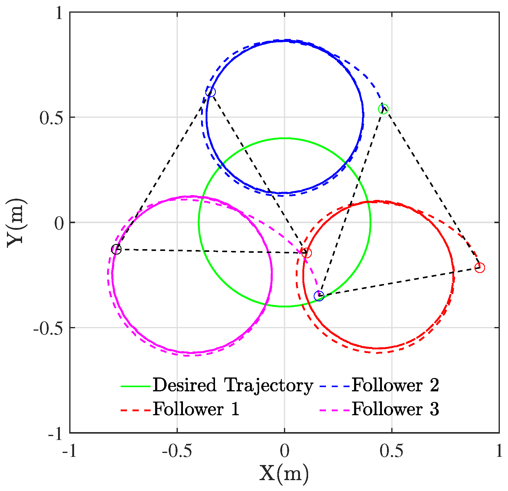
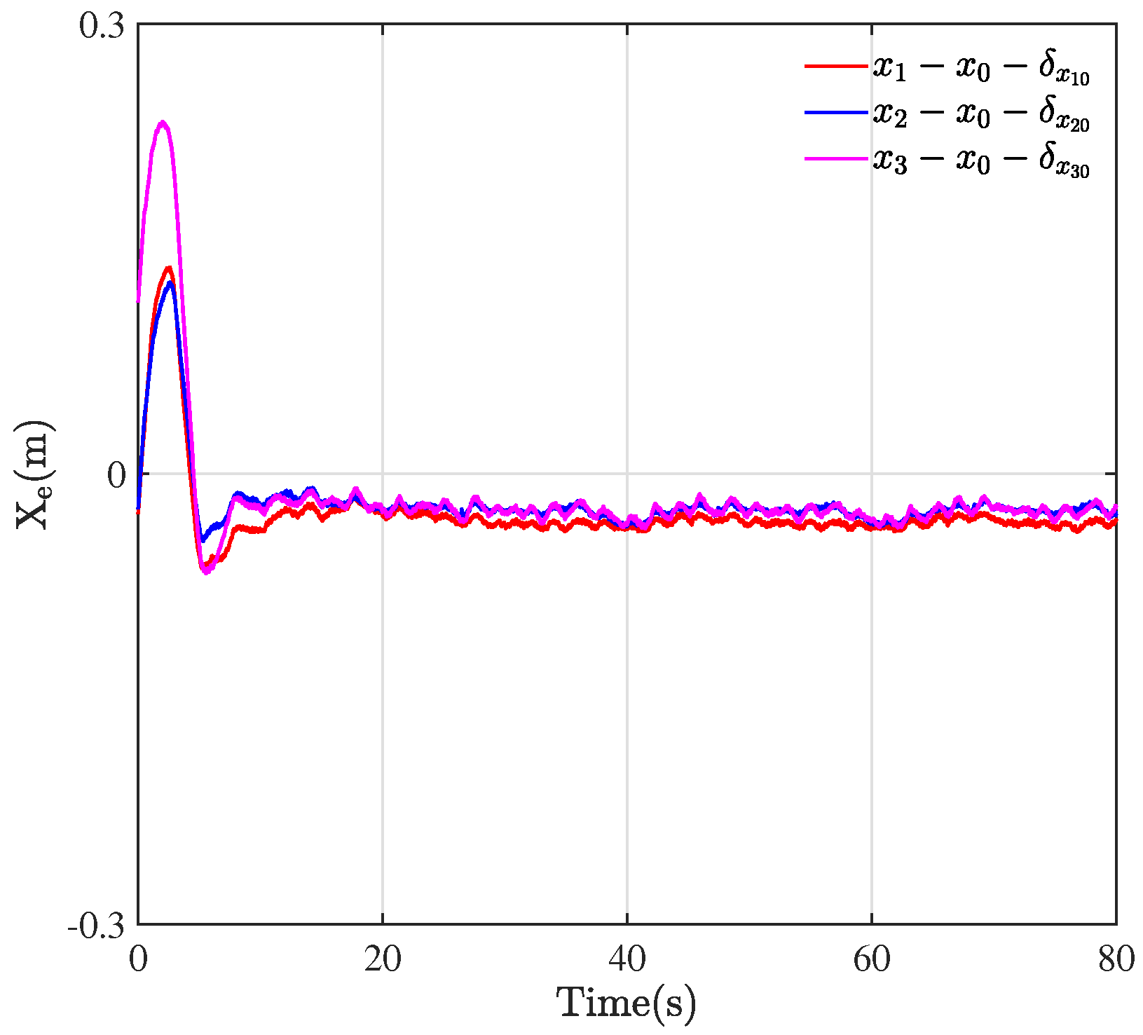
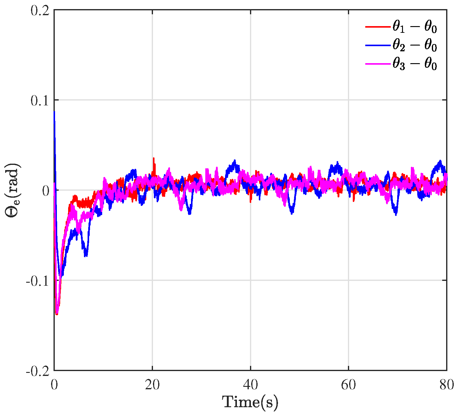
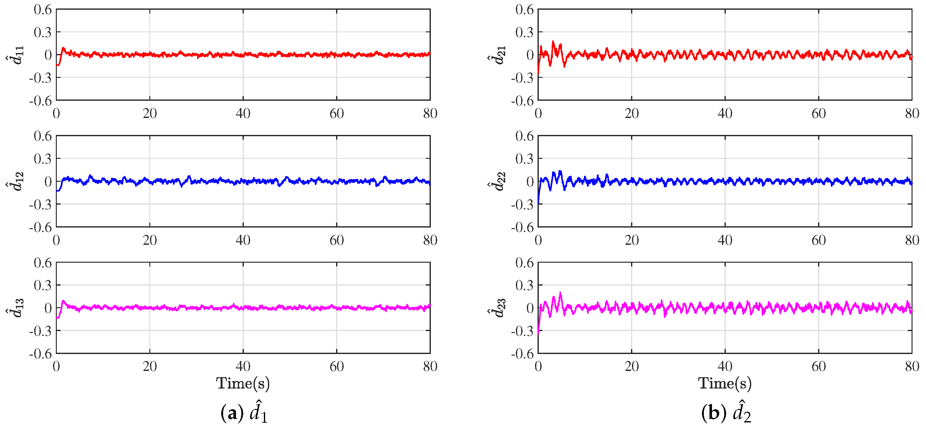
5. Experimental Results

To confirm the efficiency of the proposed control scheme, the formation trajectory tracking experiment is implemented on the QBot 2e mobile robot platform. The configuration block diagram illustrating the control scheme and the application scenario are depicted in Figure 2. The experimental platform primarily comprises three QBot 2e robots, one central host computer, a set of infrared motion capture systems for real-time pose information acquisition, and a wireless communication router to enable wireless connectivity.

The experiment aims to realize that three QBot 2e robots start from random positions and maneuver to achieve a stable formation in the shape of an equilateral triangle. The robots autonomously converge to form a stable equilateral triangle formation and track a circular trajectory with a predefined radius of 0.4 m.

The directed topology graph of multiple WMRs is depicts in Figure 3, with the leader identified as 0 and three followers labeled as 1, 2, and 3. The connected topology indicates that only part of the followers have access to information transmitted by the leader. In the experiment, the relevant physical parameters of QBot 2e are given as $m=4\mathrm{kg}$, $J=2.5$ $\mathrm{kg}·{\mathrm{m}}^2$. The parameters of the designed fixed-time disturbance observers for two subsystems are selected as ${\gamma }_1=1$, ${\gamma }_2=0.01$, ${\gamma }_3=1$, ${\gamma }_4=0.01$, ${ϵ}_1=0.1$, ${ϵ}_2=0.1$. And the main parameters of the proposed distributed formation controllers for multi WMRs are given by $k_1=4.5$, $k_2=4$, $k_3=2$, $k_4=74$, $k_5=4$, ${\alpha }_1=0.01$, ${\beta }_1=1$, ${\alpha }_2=0.01$, ${\beta }_2=1$, $p_1=0.53$, $q_1=1.3$, $p_2=0.53$, $q_2=1.3$.

Figure 4 plots the results of the formation tracking experiment of three WMRs, where the green circle represents the desired trajectory of the virtual leader. The red, blue, and cyan circles portray the trajectory of three followers labeled by 1, 2, and 3. The black dashed lines depict the configurations of three QBot 2e robots at their initial positions, which form an irregular triangle.

Through the designed control framework, it can be observed that, once the system stabilizes, the entire formation system of WMRa forms the desired equilateral triangle. Moreover, they all track the expected circular trajectory with a radius of $0.4$ m. Figure 5, Figure 6 and Figure 7 illustrate the experimental tracking errors $X_e$, $Y_e$, and ${\Theta }_e$ between the virtual leader and followers. As can be observed from the figure, the tracking error of the formation system can be stabilized and converged to a smaller value around 0 in about 15 s, which indicates a fast convergence rate, high accuracy, and small variability. This is achieved through the variable coefficient and variable exponent terms proposed by the controller (26). Furthermore, the efficacy of the proposed formation control scheme is validated through the results of tracking errors.

As depicted in Figure 8, the control inputs in the experiments can oscillate within an appropriate range by utilizing the designed formation protocols. At the same time, the stable control inputs ensure that each WMR can establish a formation configuration while tracking the desired trajectory of the leader.

The observed values ${\widehat{d}}_1$ and ${\widehat{d}}_2$ in the experimental environment are provided in Figure 9. In this experiment, the external disturbances may arise from factors such as uneven laboratory ground, wind effects, sensor measurement errors, and so on. The data displayed in Figure 9 clearly show that the error states are bounded after the system is stable. The observers demonstrate a high degree of accuracy in their estimation of the disturbances in the external environment.

6. Conclusions

This article investigates the problem of distributed fixed-time tracking control for MASs and applies it to a multi-WMR system. Firstly, a fixed-time disturbance observer is designed for a third-order continuous integration system with external disturbances, which can effectively attenuate the chattering phenomenon. Then, a distributed controller is devised to achieve the formation tracking of a third-order MAS by combining the integral sliding-mode methodology. Finally, the designed control scheme is applied to a mobile robot platform for experimental validation. Nevertheless, the design and experimental implementation of the entire control method rely on the assumption of ideal communication conditions. Further study will focus on communication delays in formation control for MASs.

References

1. Hu, Q.; Shi, Y.; Wang, C. Event-based formation coordinated control for multiple spacecraft under communication constraints. IEEE Trans. Syst. Man Cybern. Syst. 2021, 51, 3168–3179. [Google Scholar] [CrossRef]
2. Gong, W.; Li, B.; Yang, Y.; Xiao, B.; Ran, D. Leader-following output-feedback consensus for second order multiagent systems with arbitrary convergence time and prescribed performance. ISA Trans. 2023, 141, 251–260. [Google Scholar] [CrossRef]
3. Li, B.; Liu, H.; Ahn, C.K.; Gong, W. Optimized intelligent tracking control for a quadrotor unmanned aerial vehicle with actuator failures. Aerosp. Sci. Technol. 2024, 144, 108803. [Google Scholar] [CrossRef]
4. Sun, Z.; Liu, Q.; Huang, N.; Yu, C.; Anderson, B.D.O. Cooperative event-based rigid formation control. IEEE Trans. Syst. Man Cybern. Syst. 2021, 51, 4308–4320. [Google Scholar] [CrossRef]
5. Yan, Z.; Zhang, M.; Zhang, C.; Zeng, J. Decentralized formation trajectory tracking control of multi-AUV system with actuator saturation. Ocean Eng. 2022, 255, 111423. [Google Scholar] [CrossRef]
6. Maghenem, M.; Loria, A.; Nuno, E.; Panteley, E. Consensus-based formation control of networked nonholonomic vehicles with delayed communications. IEEE Trans. Autom. Control 2021, 66, 2242–2249. [Google Scholar] [CrossRef]
7. Liang, D.; Wang, C.; Cai, X.; Li, Y.; Xu, Y. Distributed fixed-time leader-following consensus tracking control for nonholonomic multi-agent systems with dynamic uncertainties. Neurocomputing 2021, 430, 112–120. [Google Scholar] [CrossRef]
8. Cui, Y.; Cao, L.; Gong, X.; Basin, M.V.; Shen, J.; Huang, T. Resilient output containment control of heterogeneous multiagent systems against composite attacks: A digital twin approach. IEEE Trans. Cybern. 2023. [Google Scholar] [CrossRef] [PubMed]
9. Li, B.; Gong, W.; Yang, Y.; Xiao, B. Distributed fixed-time leader-following formation control for multi-quadrotors with prescribed performance and collision avoidance. IEEE Trans. Aerosp. Electron. Syst. 2023, 59, 7281–7294. [Google Scholar] [CrossRef]
10. Bhat, S.; Bernstein, D. Finite-time stability of continuous autonomous systems. SIAM J. Control Optim. 2000, 38, 751–766. [Google Scholar] [CrossRef]
11. Zuo, Z.; Tie, L. A new class of finite-time nonlinear consensus protocols for multi-agent systems. Int. J. Control. 2014, 87, 363–370. [Google Scholar] [CrossRef]
12. Du, H.; Wen, G.; Cheng, Y.; He, Y.; Jia, R. Distributed finite-time cooperative control of multiple high-order nonholonomic mobile robots. IEEE Trans. Neural Netw. Learn. Syst. 2017, 28, 2998–3006. [Google Scholar] [CrossRef]
13. Zhang, J.; Fu, Y.; Fu, J. Adaptive finite-time optimal formation control for second-order nonlinear multiagent systems. IEEE Trans. Syst. Man Cybern. Syst. 2023, 53, 6132–6144. [Google Scholar] [CrossRef]
14. Wei, C.; Li, Y.; Yin, Z.; Liang, Z.; Feng, J. On finite-time anti-saturated proximity control with a tumbling non-cooperative space target. Space Sci. Technol. 2023, 3, 0045. [Google Scholar] [CrossRef]
15. Ou, M.; Du, H.; Li, S. Finite-time tracking control of multiple nonholonomic mobile robots. Int. J. Robust Nonlinear Control 2012, 349, 2834–2860. [Google Scholar] [CrossRef]
16. Tran, Q.V.; Trinh, M.H.; Zelazo, D.; Mukherjee, D.; Ahn, H.S. Finite-time bearing-only formation control via distributed global orientation estimation. IEEE Trans. Control Netw. Syst. 2019, 6, 702–712. [Google Scholar] [CrossRef]
17. Wang, D.; Zong, Q.; Tian, B.; Wang, F.; Dou, L. Finite-time fully distributed formation reconfiguration control for UAV helicopters. Int. J. Robust Nonlinear Control 2018, 28, 5943–5961. [Google Scholar] [CrossRef]
18. Zhu, C.; Huang, B.; Su, Y.; Zhou, B.; Zhang, E. Finite-time time-varying formation control for marine surface vessels. Ocean. Eng. 2021, 239, 109817. [Google Scholar] [CrossRef]
19. Polyakov, A. Nonlinear feedback design for fixed-time stabilization of linear control systems. IEEE Trans. Autom. Control 2012, 57, 2106–2110. [Google Scholar] [CrossRef]
20. Liu, H.; Li, B.; Xiao, B.; Ran, D.; Zhang, C. Reinforcement learning-based tracking control for a quadrotor unmanned aerial vehicle under external disturbances. Int. J. Robust Nonlinear Control 2023, 33, 10360–10377. [Google Scholar] [CrossRef]
21. Jiang, B.; Hu, Q.; Friswell, M.I. Fixed-time rendezvous control of spacecraft with a tumbling target under loss of actuator effectiveness. IEEE Trans. Aerosp. Electron. Syst. 2016, 52, 1576–1586. [Google Scholar] [CrossRef]
22. Liu, J.; Sun, M.; Chen, Z.; Sun, Q. Output feedback control for aircraft at high angle of attack based upon fixed-time extended state observer. Aerosp. Sci. Technol. 2019, 95, 105468. [Google Scholar] [CrossRef]
23. Ye, D.; Zou, A.M.; Sun, Z. Predefined-time predefined-bounded attitude tracking control for rigid spacecraft. IEEE Trans. Aerosp. Electron. Syst. 2022, 58, 464–472. [Google Scholar] [CrossRef]
24. Cao, L.; Xiao, B.; Golestani, M.; Ran, D. Faster fixed-time control of flexible spacecraft attitude stabilization. IEEE Trans. Ind. Inform. 2020, 16, 1281–1290. [Google Scholar] [CrossRef]
25. An, S.; Wang, L.; He, Y. Robust fixed-time tracking control for underactuated AUVs based on fixed-time disturbance observer. Ocean Eng. 2022, 266, 112567. [Google Scholar] [CrossRef]
26. Zuo, Z.; Tian, B.; Defoort, M.; Ding, Z. Fixed-time consensus tracking for multiagent systems with high-order integrator dynamics. IEEE Trans. Autom. Control 2018, 63, 563–570. [Google Scholar] [CrossRef]
27. Ou, M.; Sun, H.; Zhang, Z.; Li, L. Fixed-time trajectory tracking control for multiple nonholonomic mobile robots. Trans. Inst. Meas. Control 2021, 43, 1596–1608. [Google Scholar] [CrossRef]
28. Liu, Y.; Zhang, F.; Huang, P.; Lu, Y. Fixed-time consensus tracking for second-order multiagent systems under disturbance. IEEE Trans. Syst. Man Cybern. Syst. 2021, 51, 4883–4894. [Google Scholar] [CrossRef]
29. Chen, Y.; Zhu, B. Distributed fixed-time control of high-order multi-agent systems with non-holonomic constraints. J. Franklin Inst. 2021, 358, 2948–2963. [Google Scholar] [CrossRef]
30. Ma, L.; Wang, Y.L.; Fei, M.R.; Pan, Q.K. Cross-dimensional formation control of second-order heterogeneous multi-agent systems. ISA Trans. 2022, 127, 188–196. [Google Scholar] [CrossRef]
31. Zhang, G.; Wang, Y.; Wang, J.; Chen, J.; Qian, D. Disturbance observer–based super-twisting sliding mode control for formation tracking of multi-agent mobile robots. Meas. Control 2020, 53, 908–921. [Google Scholar] [CrossRef]
32. Cheng, W.; Zhang, K.; Jiang, B.; Ding, S.X. Fixed-time fault-tolerant formation control for heterogeneous multi-agent systems with parameter uncertainties and disturbances. IEEE Trans. Circuits Syst. I Reg. Pap. 2021, 68, 2121–2133. [Google Scholar] [CrossRef]
33. Jenabzadeh, A.; Safarinejadian, B. Distributed estimation and control for nonlinear multi-agent systems in the presence of input delay or external disturbances. ISA Trans. 2020, 98, 198–206. [Google Scholar] [CrossRef] [PubMed]
34. Olfati-Saber, R.; Murray, R. Consensus problems in networks of agents with switching topology and time-delays. IEEE Trans. Autom. Control 2004, 49, 1520–1533. [Google Scholar] [CrossRef]
35. Polycarpou, M.; Ioannou, P. A robust adaptive nonlinear control design. Automatica 1996, 32, 423–427. [Google Scholar] [CrossRef]
36. Chevillard, S. The functions erf and erfc computed with arbitrary precision and explicit error bounds. Inf. Comput. 2012, 216, 72–95. [Google Scholar] [CrossRef]
37. Bagul, Y.J.; Chesneau, C. Sigmoid functions for the smooth approximation to the absolute value function. Moroccan J. Pure Appl. Anal. 2021, 7, 12–19. [Google Scholar] [CrossRef]
Figure 1. Leader–follower formation model of multi-WMRs.
Actuators 13 00068 g001
Figure 2. Frame of control scheme and QBot 2e platform.
Actuators 13 00068 g002
Figure 3. Communication topology among WMRs.
Actuators 13 00068 g003
Figure 4. Trajectory tracking for multiple WMRs.
Actuators 13 00068 g004
Figure 5. Tracking errors of X e .
Actuators 13 00068 g005
Figure 6. Tracking errors of Y e .
Actuators 13 00068 g006
Figure 7. Tracking errors of Θ e .
Actuators 13 00068 g007
Figure 8. Response curves of control inputs in experiment.
Actuators 13 00068 g008
Figure 9. External disturbance estimation in experiment.
Actuators 13 00068 g009
Disclaimer/Publisher’s Note: The statements, opinions and data contained in all publications are solely those of the individual author(s) and contributor(s) and not of MDPI and/or the editor(s). MDPI and/or the editor(s) disclaim responsibility for any injury to people or property resulting from any ideas, methods, instructions or products referred to in the content.