Abstract
A dynamic LC trajectory planning algorithm based on the modified driving risk field is proposed to address the issue of dynamic changes during the lane-changing (LC) process. First, a modified driving risk field (MDRF) model is constructed for LC scenarios. Then, according to the state of the target vehicle and discrete sampling points, a series of LC candidate trajectories were generated based on the quintic polynomial. After eliminating candidate trajectories that do not meet the constraints, the MDRF was utilized as a safety evaluation function. Additionally, comfort and smoothness evaluation functions were combined to evaluate candidate LC trajectories in order to obtain the optimal LC reference trajectory. Then, this paper proposes a dynamic LC trajectory planning algorithm, addressing the challenges of complex traffic scenarios and dynamic changes in adjacent vehicle states. Utilizing the optimal reference trajectory as a basis, a dynamic segmented algorithm is applied to the x–t and y–x curves, constructing an optimized objective function that considers the MDRF. Under multiple constraints, including the continuity and smoothness of the lateral and longitudinal trajectories, the penalty function approach is employed to solve the optimization objective function, yielding the optimal LC trajectory adapted to real-time changes in the traffic state. Finally, the proposed dynamic LC trajectory planning algorithm was validated under four different scenarios by using MATLAB 2023b. The simulation results indicate the safety, continuity, and dynamic feasibility of the proposed algorithm. Moreover, it demonstrates strong adaptability and flexibility in challenging dynamic LC scenarios.
1. Introduction
Lane changing (LC) and following behaviors are the most prevalent driving behaviors. Compared to the following behaviors, LC behaviors require transitioning from the current lane to the target lane, making the process more complex and more prone to collisions with adjacent vehicles [1,2]. Relevant research has demonstrated that 70% of traffic accidents are caused by human error, with LC behavior being one of the primary reasons for various accidents [3]. Based on statistical data, traffic accidents caused by LC maneuvers account for approximately 4% to 10% of all traffic accidents, leading to about 10% of total traffic delays [4]. Intelligent and connected vehicles (ICVs) can enhance travel experience, improve driving safety, reduce traffic accidents, and mitigate the likelihood of traffic congestion [5,6]. With the development of ICVs, it is widely believed in the industry that they provide a crucial solution to address issues such as traffic safety, congestion, and pollution. ICVs have the potential to reduce over 50% of traffic accidents [7]. According to the definitions by the Society of Automotive Engineers (SAE) [8], currently most automobiles are at level 2 (L2). L2 represents partial automation, where auto lane change (ALC) systems are vital components of L2 advanced driving assistance systems (ADAS) used in specific scenarios, enabling vehicles to perform lane changes independently within predefined circumstances [9]. LC trajectory planning is a critical component of ALC systems [10]. It generates an LC path that avoids collisions with adjacent vehicles, providing significant assurance for efficient and safe vehicle maneuvering. It has garnered significant attention from researchers in related fields.
However, in real-road environments, traffic conditions are highly complex and constantly changing. Vehicles equipped with ADAS systems face challenges in assessing dynamic environmental risks, especially in highly dynamic and complex scenarios [11]. The LC trajectory cannot be adjusted based on real-time traffic conditions, which consequently lead to frequent traffic accidents. The National Highway Traffic Safety Administration (NHTSA) reports that in 2023, there were a total of 367 traffic accidents that involved L2-level ADAS in the US. Among which 51.86% involved collisions resulting from lane changing or merging [12]. As a result, the industry has repeatedly postponed the timeline for attaining complete autonomy in highly dynamic and complex scenarios [13]. Consequently, it is imperative for the LC vehicles to adapt to the intricate and fluctuating traffic environments by dynamically adjusting their trajectories based on information such as the positions, speeds, and accelerations of adjacent vehicles, thereby ensuring the safety of LC maneuvers.
Given this, this paper proposes a dynamic LC trajectory planning algorithm for ICVs in response to the dynamically changing surrounding environments. This algorithm aims to provide ICVs with the capability of real-time adaptation to varying traffic environments, accurately anticipate potential collision risks, and quickly make optimal trajectory adjustments. Firstly, referring to the artificial potential field (APF) theory, a modified driving risk field (MDRF) for LC scenarios is constructed, taking into account the size, position, velocity, and acceleration of adjacent vehicles. Next, employing a quintic polynomial, the LC trajectory planning is decomposed into path planning and velocity planning, generating LC trajectories clusters. Utilizing the MDRF, an evaluation function is constructed to select the reference LC trajectory. Subsequently, based on the reference LC trajectory, the optimal trajectory is dynamically segmented and optimized. An optimization objective function based on the MDRF is constructed, which is constrained by start and end points, x–t curve, y–x curve, and smoothness conditions. And the penalty function method is applied to solve this optimization problem, yielding the optimal LC trajectory. Finally, MATLAB simulations are constructed to validate the effectiveness of the proposed algorithm.
The overall structure of this paper is organized as follows: Section 2 summarizes the relevant theoretical methods in the research field of driving risk field (DRF) and LC trajectory optimization. Section 3 constructs an MDRF specifically for LC scenarios, evaluating real-time potential LC risks. In Section 4, a cluster of LC trajectories is generated based on quintic polynomials, from which a reference LC trajectory is selected. Section 5 proposes a dynamic optimizing algorithm for LC trajectories. Finally, Section 6 conducts simulations to validate the proposed algorithm under various scenarios.
2. Literature Review
In recent years, the safety of the traffic participants, especially the ICVs, has attracted significant concern. Trajectory planning and risk assessment methodologies are the main research directions. Risk assessment, a critical component for decision making and ensuring the secure operation of ICVs in complex traffic scenarios, involves evaluating the potential influence of diverse traffic elements within the traffic environment on the operational safety of these vehicles.
The field-based driving risk assessment aligns more closely with the intrinsic nature of how drivers perceive risks [14]. It can assimilate data regarding the vehicles’ dynamic conditions and traffic environment, especially during interactions among multiple vehicles. The concept of artificial potential fields (APFs), introduced by Khatib in 1986, marked a significant advancement in this field. Initially applied to investigate robot path planning and obstacle avoidance, APF has been widely adopted in collision avoidance and path planning for autonomous vehicles [15]. Building upon the foundational principles of APF, Wang et al. innovatively proposed the driving risk field (DRF) model and applied it to vehicle risk assessment in complex road traffic environments [16]. Matinez and Jimenez take into account the forward, side, and diagonal potentials to simulate interactions between the vehicles and environmental elements [17]. The DRF differs from traditional vehicle dynamics and kinematics-based risk assessment methods by quantifying the interactive effects between vehicles and surrounding elements, such as pedestrians, adjacent vehicles, road conditions, and infrastructure, into a risk field distribution during driving [18]. For risk perception, early warning, and decision making in ITS, DRF provides more comprehensive and dynamic theoretical support [19]. Subsequent research has enhanced the DRF by considering factors such as minimum safety distance [20], vehicle motion direction [21], acceleration, and steering angle. Li et al. [22] assessed the LC risks and presented the distribution of the DRF under different motion states, summarizing the safe distance required at the end of the LC process. Mullakkal-Babu et al. [23] developed an improved APF model based on the product of collision probability and expected collision energy to assess the driving risk. They further utilized this model to predict the collision probability with adjacent vehicles and evaluated the risk for different scenarios by selecting either a single time step or multiple time steps. Chen et al. [24] computed the risk at each time point during the LC process based on the risk indicators derived from the DRF. They then generated an LC risk field and applied dynamic time warping (DTW) and K-means clustering algorithms to classify the LC risk profiles into several categories. The DRF contributes to designing and understanding the risk distribution and safety orientation in dynamic traffic environments. It has facilitated the simulation of risk fields for ICVs in intricate traffic scenarios, enabling a deeper analysis and optimization of driving safety. Li et al. [25] suggested a novel dynamic driving risk potential field model that completely accounts for the dynamic influence of the vehicle’s steering angle and acceleration. The distribution of risk fields is impacted by acceleration and steering angle. Son and Kim [26] used a cooperation concept to present an innovative approach to assess the rear-end collision risk for an autonomous LC system, offering a more flexible and proactive method compared to previous methods. Zhang et al. [27] investigated the driving risk pulse field model by risk pulse energy for cars following, which include both basic and random risk energies. The model assesses the overall risk performance and total risk level from vector and scalar perspectives, which includes the properties and motion states of vehicles, pedestrians, obstacles, etc., such as speed and acceleration.
In terms of LC trajectory planning and optimization, a multitude of innovative approaches have been proposed to enhance the safety and efficiency of autonomous vehicles. Yang et al. [28] employed an improved APF method to assess path risk, accounting for the driver’s style and reaction time. Finally, the optimal path was selected based on a comprehensive consideration of LC efficiency and comfort. Zuo et al. [29] proposed a local path planning method that combines Model Predictive Control (MPC) with APF. They incorporated the potential field function into the cost function, transforming the local path planning problem into a typical MPC optimization problem. And the PSO strategy was employed for the optimal path. Matinez et al. [17] proposed the algorithm for lateral and longitudinal planning based on the potential models. The lateral planning algorithm calculates the steering angle based on the total lateral potential, which includes contributions from side and diagonal potentials. While the longitudinal planning algorithm determines the vehicle’s speed based on the obstacles and the road conditions. Li et al. [30] proposed an efficient LC path planning method that leverages prior road information to optimize the selection of sampling points, enhancing the algorithm’s real-time performance and reducing the number of candidate paths. Beyond the sampling points, additional intermediate nodes and target points were introduced to address the issue of continuous LC, thereby enabling ICVs to execute complex maneuvers. Wang et al. [31] proposed a hybrid trajectory planning method based on sampling and numerical optimization methods. Initially, they used sampling methods to decompose path velocity and generate collision-free candidate trajectories. Considering factors such as curve smoothness, collision risk, and travel time, the optimal trajectory was determined. Finally, within the spatiotemporal constraints, sequential quadratic programming (SQP) was applied to optimize the trajectory, guaranteeing safety, stability, and comfort. Ding et al. [32] proposed a time-based quintic polynomial algorithm to derive an LC reference trajectory that satisfies multiple criteria, including safety, LC duration, driving distance, and comfort. They introduced LC constraints induced by adjacent vehicles and ultimately minimized LC duration, driving distance, driving comfort, and fuel consumption to compute the optimal LC trajectory that eliminates potential collisions. Yu et al. [33] proposed the LC decision-making model for ICVs in a mixed traffic environment based on multi-player dynamic game theory. This model introduced an overtaking expectation parameter to measure the utility of following vehicles and employed a hybrid splitting algorithm to solve the Nash equilibrium solution in multi-player games, thereby achieving the optimal solution for LC decisions. Luo et al. [34] employed hidden Markov models (HMMs) to assess adjacent vehicles, calculating the magnitude of obstacle vehicles’ longitudinal and lateral potential field strength. By utilizing HMMs with real-time trajectory prediction methods, the feasible collision avoidance paths were obtained. Wang et al. [35] proposed a combined optimization method based on NSGA-II and TOPSIS to solve the multi-objective optimization problem of LC trajectory algorithms. Under the consideration of LC constraints, feasible trajectory clusters were generated based on the quintic polynomial to ensure the comfort, stability, and effectiveness of the LC process. The NSGA-II algorithm was employed to optimize longitudinal displacement and LC duration. A continuous ordered weighted averaging operator was introduced to calculate weights for three objective optimization functions. Finally, the TOPSIS algorithm was applied to obtain the optimal LC trajectory. Liu et al. [36] aimed to accomplish dependable real-time avoidance of both static and moving obstacles in the situation involving multi-vehicles interacting on a constructed road and provided a least action principle to present a hierarchical lane-changing trajectory planner. Feng et al. [37] addressed the interaction effects between the ego vehicle and adjacent vehicles in the dynamic road environment and suggested an LC decision making and trajectory planning method using the GCNs and multi-segment polynomial curve optimization. Zhu et al. [38] explored the integration of dynamic vehicle trajectories, vehicle safety factors, static traffic environments, and actuator constraints to improve cooperative intent modeling. And proposed a cooperative intent multi-layer graph neural network (CMGNN) model for a more comprehensive approach to trajectory planning. Nie et al. [39] proposed a framework to dynamically plan LC trajectory for autonomous buses. The planning and replanning algorithm is optimized in the safe range of longitudinal length. And the optimization is aimed at generating a real-time reference trajectory that takes into account the buses’ yaw, roll dynamics, and LC efficiency.
In the realm of LC trajectory planning and optimization, significant strides have been made to enhance the rationality and comfort of trajectories, particularly under scenarios where adjacent vehicles are assumed to be in constant conditions. Furthermore, the computational intensity of some methods, such as those utilizing model predictive control (MPC) or sequential quadratic programming (SQP), may exceed the processing capabilities of onboard vehicle systems, thereby limiting their practicality for real-time decision making. The need for dynamic LC trajectory planning that can adapt to the uncertainties and complexities of traffic environments is therefore paramount. In light of these limitations, this paper introduces a dynamic LC trajectory planning algorithm designed to respond to the interactive states between the LC vehicle and adjacent vehicles in real time. The proposed algorithm aims to overcome the aforementioned challenges by adjusting LC strategies across different phases of the LC process, thereby planning trajectories that are not only efficient and smooth but also minimize potential risks. This approach is intended to enable intelligent connected vehicles (ICVs) to better navigate the complexities of real-world road conditions, marking a significant step towards the practical implementation of autonomous driving technologies in varied traffic scenarios.
3. Modeling of Modified Driving Risk Field
3.1. LC Scenario
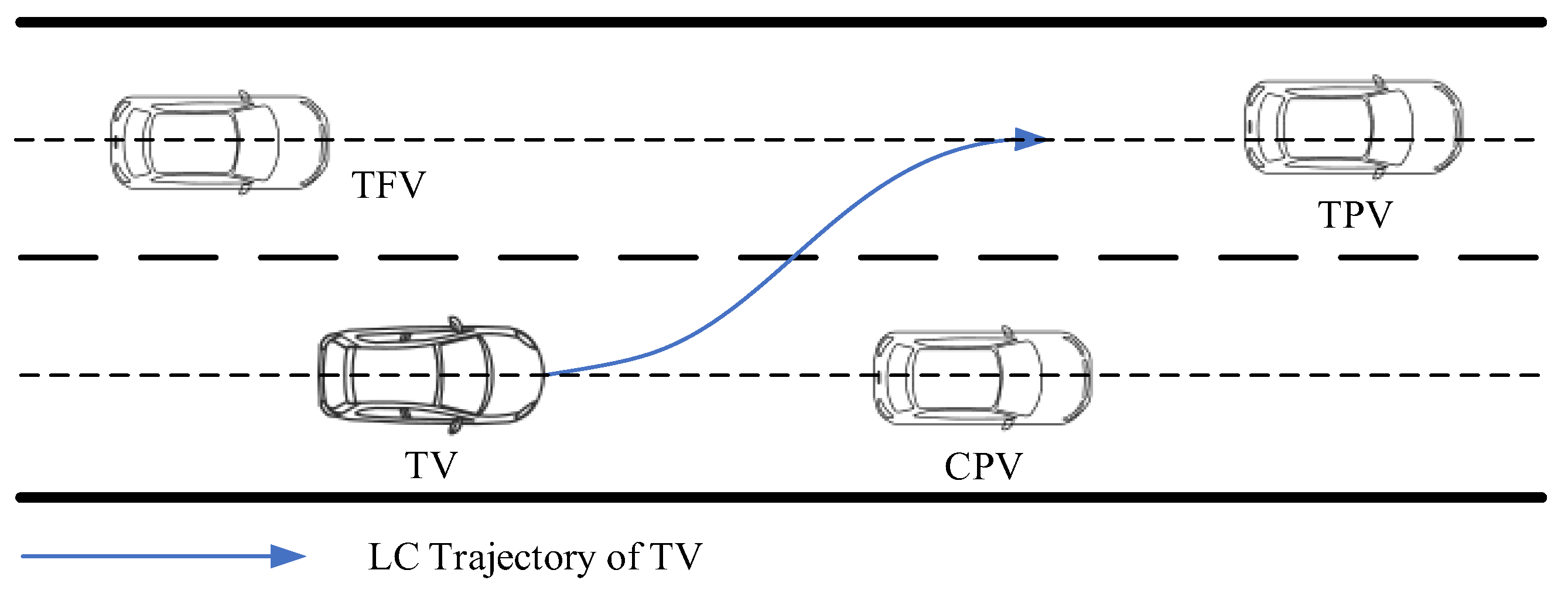
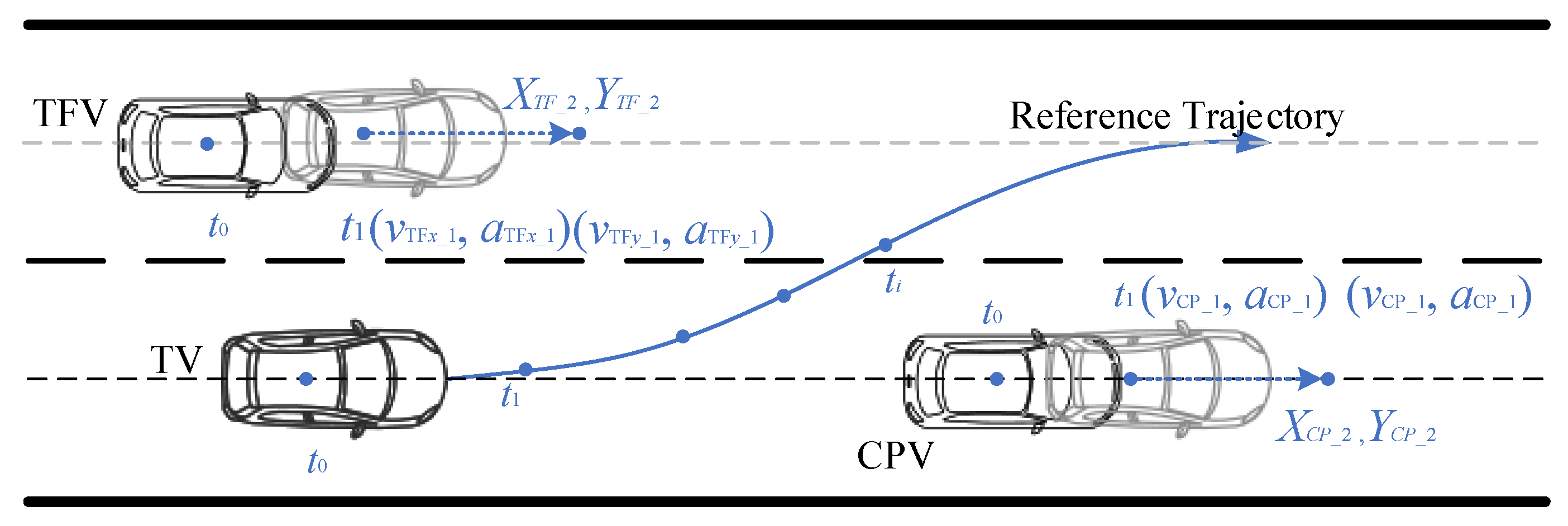
The typical LC scenario for the ICVs in a multi-lane highway environment is illustrated in Figure 1. TV is the target vehicle intending to change lane, CPV is the current-lane preceding vehicle, TPV is the target-lane preceding vehicle, and TFV is the target-lane preceding vehicle.
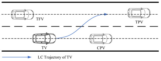
Figure 1.
Illustration of the typical LC scenario.
3.2. Modified Driving Risk Field Model
The MDRF for LC scenarios includes the road risk field, static risk field, and dynamic risk field. The road risk field mainly consists of the roadside risk field and the lane centerline risk field. The static risk field primarily considers the static attributes of adjacent vehicles, incorporating vehicle size, the distance to the adjacent vehicles, and the direction of vehicles approaching the TV. The dynamic risk field mainly encompasses the impact of the dynamic characteristics of adjacent vehicles and the relative dynamic features of the TV.
3.2.1. Road Risk Field
Highway is the typical structured road, on which the roadside markings are used to regulate and restrict the longitudinal (Y direction) movement of vehicles, ensuring driving safety [40]. Depending on the different impacts of roadside markings and lane centerlines on risk, the road risk field includes the roadside risk field and the lane centerline risk field.
- (1)
- Roadside Risk Field
Higher risk field strength results from an increase in the potential risk when the TV drives up to the roadside [41]. Since the roadside cannot be crossed and the roadside risk field does not vary dynamically, it is solely determined by the vehicle’s longitudinal position. The roadside risk field can be calculated using the following formulas:
where Aroad_b is the coefficient of the roadside risk field, yroad_b is the longitudinal coordinate of the boundary line, and σroad_b and c1 are the shape coefficients.
- (2)
- Lane Centerline Risk Field
The lowest risk for TV is when it remains on the lane centerline, while the highest risk is when it crosses the lane line [42]. The lane centerline risk field does not change over time and is only related to the vehicle’s longitudinal position. Therefore, the lane centerline risk field is:
where n is the number of lanes, Aroad_c is the coefficient of lane centerline risk field, yroad_c is the longitudinal position of the lane centerline, and σroad_c and c2 are the are the shape coefficients.
- (3)
- Road Risk Field
Therefore, the road risk field is the combination of the roadside risk field and the lane centerline risk field:
3.2.2. Static Risk Field
Three factors primarily influence the static risk field, which focuses on the static attributes of adjacent vehicles: (1) the relative distance between the TV and adjacent vehicles; (2) the direction in which the TV approaches the adjacent vehicles; and (3) the dimensions of the adjacent vehicles.
First, the smaller the relative distance between the TV and adjacent vehicles, the greater the possibility of collision and the stronger the static risk field. Second, considering the actual motion characteristics of vehicles, their traveling direction is limited; that is, the longitudinal speed of vehicles is usually much smaller than the lateral speed [43]. Therefore, laterally, the static risk field of adjacent vehicles has a greater impact range, while longitudinally, the impact range of the static risk field is smaller. In addition, taking into account the influence of the adjacent vehicles’ dimensions, the larger the vehicle size, the relatively higher the risk it poses.
Due to the rapid decrease in field strength with increasing distance in traditional first-order central moment two-dimensional Gaussian functions when describing the static risk field of vehicles [44]. It implies the risk-field strength at the edge of the vehicle will rapidly decrease. However, this situation does not align with reality. In fact, the edge of the vehicle also poses a higher risk to the TV. In contrast, using two-dimensional Gaussian functions with high-order central distance can flatten the peak of the function. This results in a smaller difference in field strength between the edge and the center of the vehicle, better reflecting the distribution of the vehicle’s static risk field.
Furthermore, high-order Gaussian functions can accurately describe the impact of changes in the relative position between TV and adjacent vehicles on the field strength and can control the shape of the risk field by adjusting the high-order terms, making the lateral and longitudinal risk distribution of the vehicle more consistent with the perceived risk during actual driving. In conclusion, high-order Gaussian functions can better reflect the influence of relative position, directional differences, and vehicle dimensions on the risk field. The static risk field can be formulated as Equation (4).
where (x, y) is the coordinate of TV, (xj, yj) is the coordinate of the j-th adjacent vehicle, Asta is the coefficient of static risk field strength, it is a constant; β is the high-order coefficient that influences the distribution of static risk field, which can reflect the distribution in different scenarios by adjusting the value; σx and σy are the shape function of the adjacent vehicle, σx = kx × Lj, σy = ky × Wj, Lj and Wj are the length and width of the j-th adjacent vehicle, respectively; kx and ky are the dimensions coefficient of the adjacent vehicle, which adjust the influence range of the static risk field in the longitudinal and lateral directions, respectively.
3.2.3. Dynamic Risk Field
The dynamic risk field describes the evolution patterns of the potential risk between TV and the moving adjacent vehicles. It takes into account the relative distance, relative velocity, and approaching direction between TV and adjacent vehicles. As the relative distance between vehicles decreases, the risk of collision increases. Furthermore, there is a nonlinear acceleration in the rate of risk rise with decreasing distance; the rate of risk increase shows a nonlinear acceleration. In real traffic environments. The dynamic speed and approach direction of adjacent vehicles significantly affect the LC risk. For instance, the rate of increase in collision risk is faster if the following vehicle approaches at a higher speed than the leading vehicle. Conversely, the rate of decrease in collision risk is also faster if the leading vehicle accelerates away at a speed higher than the following vehicle [45]. Similarly, all other adjacent vehicles constantly changing positions during the LC process will have similar and complex interactive effects on TV.
For the moving adjacent vehicles, the highest point of the risk field strength undoubtedly lies at the vehicle’s center point. Moreover, as the distance from the vehicle’s center point increases, the risk field strength decreases, and the risk field is symmetrical on the left and right sides. That is, regardless of whether other vehicles approach from the left or right side, the risk is the same. Therefore, to comprehensively capture the influence of dynamic factors on LC risk, a dynamic risk field can be constructed using a two-dimensional Gaussian function. The two-dimensional Gaussian function can integrate multiple variables, such as relative distance and relative velocity, to accurately describe the evolution of the risk field along with the dynamics of the vehicle. The dynamic risk field is calculated as Equation (5):
where Adyn is the coefficient of dynamic risk field strength, it is a constant, α is a constant, 0 ≤ α ≤ 1, σv is a function relating the relative velocity between the moving adjacent vehicle and TV, σv = kv|vj − v|, vj is the velocity of the j-th adjacent vehicle, v is the velocity of the TV, kv is a constant greater than 0, relv is the function describing the direction of relative motion between TV and adjacent vehicle, relv = sign|vj − v|, if vj > v, relv = 1, and vj ≤ v, relv = −1.
3.2.4. Modified Driving Risk Field
In conclusion, the MDRF for TV is the sum of the road risk field, static risk field, and dynamic risk field, namely:
where U is the LC driving risk field, Usta,j(x) is the static risk field of the j-th adjacent vehicle, and Udyn,j(x) is the dynamic risk field of the j-th adjacent vehicle.
3.2.5. The Simulation of MDRF Model
According to Wang [19], and by conducting multiple tests, the values of each parameter in the MDRF model utilized in these simulations are detailed in Table 1.

Table 1.
The values of parameters in MDRF model.
To validate the field strength distributions of the road risk field, static risk field, dynamic risk field, and MDRF, simulations were conducted using MATLAB. The lane width is 3.75 m; the location, length, width, and velocity are detailed in Table 2.

Table 2.
Simulation scenario setting.
The road risk field, static risk field, and dynamic risk field are illustrated in Figure 2, Figure 3 and Figure 4.
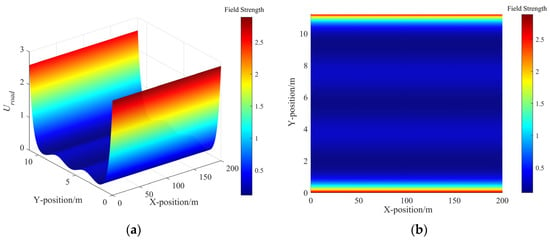
Figure 2.
The field strength distribution of road risk field: (a) the road risk field strength distribution in 3D view and (b) the road risk field strength distribution in bird view.
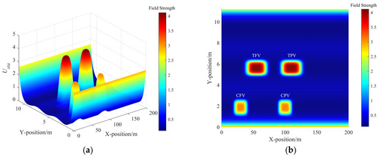
Figure 3.
The field strength distribution of static risk field. (a) The static risk field strength distribution in 3D view and (b) the static risk field strength distribution in bird view.
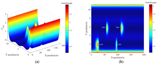
Figure 4.
The field strength distribution of dynamic risk field. (a) The dynamic risk field strength distribution in 3D view and (b) the dynamic risk field strength distribution in bird view.
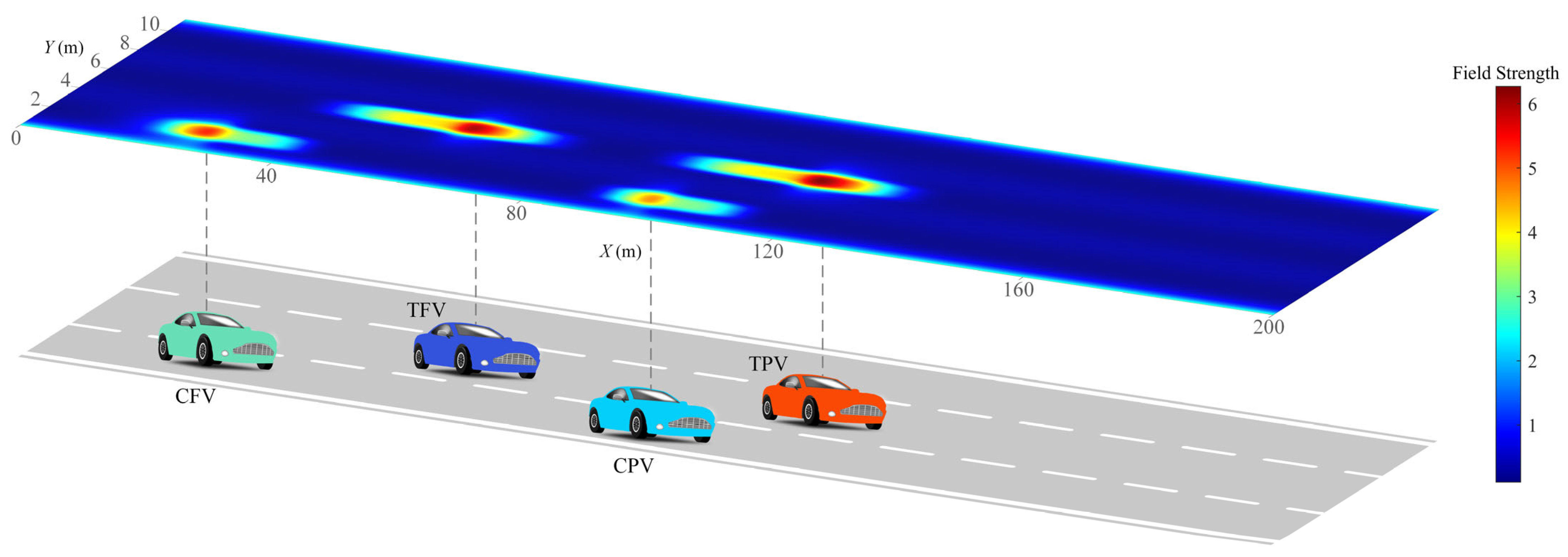
In Figure 2, the minimum risk field strength is at the centerline of the lane, while the maximum strength is at the road boundary lines. The risk field strength at the lane line is between these two extremes. The distribution of road risk fields ensures the vehicles can smoothly cross the lane line and guides the vehicles to drive near the centerline. And it can be seen in Figure 3 that the static risk field of each adjacent vehicle distributes in a shape approximating a rectangle, indicating that regardless of whether the TV approaches from the left or right, front or rear of the adjacent vehicle, it faces the same strength of static risk field. Furthermore, the coverage range of the risk field along the X-axis is greater than that along the Y-axis. In this scenario, due to the velocities of TPV and TFV being both greater than those of TV, the distribution of the dynamic risk field in Figure 4 shows a pronounced forward concentration propensity, which implies that the dynamic risk of collision is considerably high when vehicles approach from the front. Figure 5 illustrates the distribution of MDRF among the adjacent vehicles. It is evident that the risk field strengths of TPV and TFV exceed those of CPV and CFV, and the spatial extents of TPV and TFV are also greater than those of CPV and CFV. The MDRF model considers the differential impact of the adjacent vehicles, effectively capturing the gradient of risk imparted by different adjacent vehicles to TV, thus providing a nuanced assessment of the adjacent vehicular interactions.

Figure 5.
The field strength distribution of modified driving risk field.
According to the simulation results, the MDRF model comprehensively considers various influential factors such as the road, the morphological attributes, relative distances, and velocities of the adjacent vehicles on the LC risk within complex multi-vehicle motion scenarios. The MDRF model can dynamically reflect the real-time evolution of risk profiles surrounding the TV. By adjusting parameters such as the shape coefficient, the field distribution that more closely aligns with actual traffic conditions can be obtained, which can enhance the model’s applicability across diverse traffic conditions. Moreover, by mapping the risk distribution with specific spatial coordinates within the traffic environment, the MDRF model enables a more accurate and expeditious perception of dynamic changes. This mapping not only provides a visual representation but also serves as a critical input for the LC trajectory planning algorithm.
4. The LC Trajectory Dynamic Planning Algorithm Based on MDRF
4.1. Coordinate System
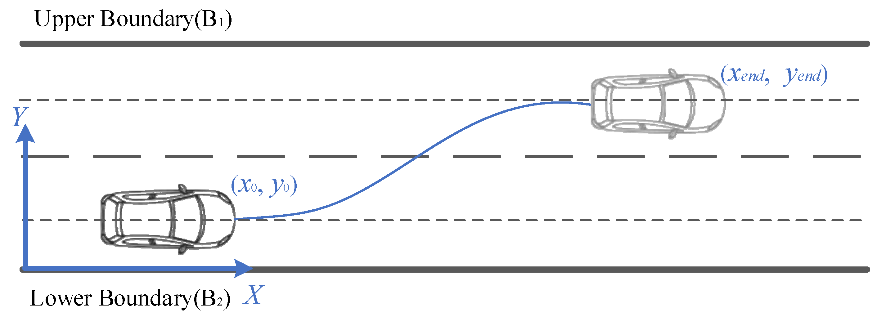
Highways are a typical structured road, characterized by their rigorous lane demarcations and stringent traffic regulations. These elements collectively establish clear boundaries and constraining conditions for vehicle operation, thereby imparting a distinct regularity and controllability to vehicle movement when traveling on highways. The upper and lower boundaries of the road are defined as B1 and B2, respectively. The coordinate system is established with the starting point of the target lane as the origin, creating a local rectangular coordinate system as shown in Figure 6. The X direction is defined as the forward direction along the road, which corresponds to the vehicle’s travel direction. The Y direction is perpendicular to the X direction. The coordinates (x0, y0) represent the position of TV at the beginning of the LC process, and the coordinates (xend, yend) represent the vehicle’s position at the end of the LC process.
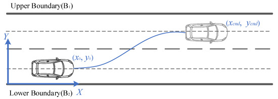
Figure 6.
Local coordinate system.
4.2. Discrete Sampling of LC Space
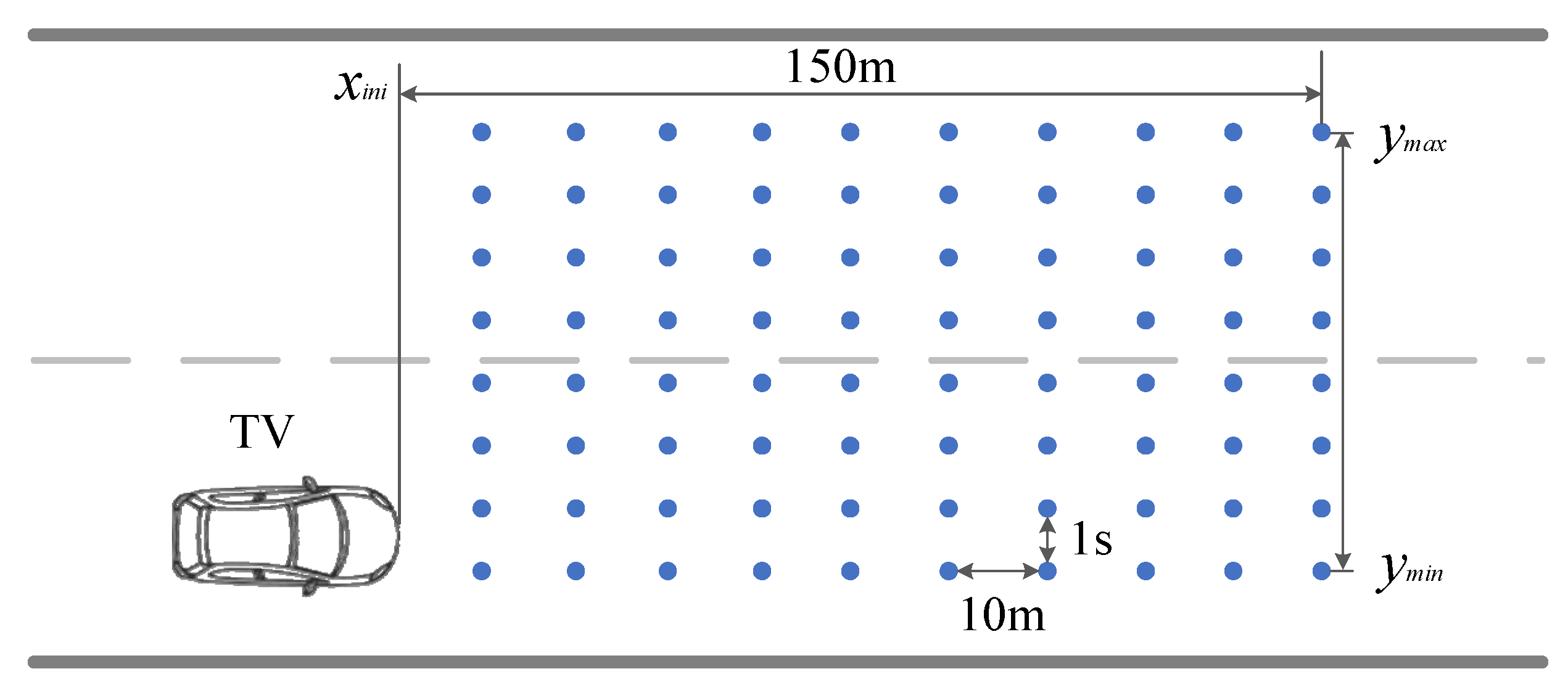
In order to avoid creating an infinite number of LC trajectories and minimize computational resources, it is necessary to discretized sample the LC space. Based on the research about the LC duration and distance, the LC distance is primarily concentrated within 150 m, and the LC duration is concentrated in 3~10 s [46,47,48]. Therefore, the sampling points are taken at an interval of ΔX = 10 m in the X direction and at an interval of Δt = 1 s in the Y direction. The sampling region ahead of the TV is shown in Figure 7. In the local rectangular coordinate system constructed in Figure 6, the length of the LC trajectory planning area is set to 150 m.
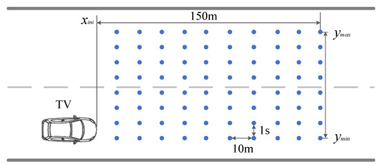
Figure 7.
Discrete sampling region and points.
In terms of lateral position, the initial position of TV at the start of the LC is xini. The discrete sampling points are as follows:
In terms of longitudinal position, the vehicle’s outer edge line should remain within the lane; the coordinate range for the vehicle center is as follows:
where Wr is the width of each lane, W is the width of the vehicle.
Therefore, within the position interval [ymin, ymax], with the sampling time interval Δt = 1 s, the longitudinal sampling points are:
4.3. Generation of LC Trajectory
4.3.1. LC Trajectory Planning Based on Quintic Polynomial
LC trajectory planning is the process of ICVs on highways, that calculates precisely a feasible trajectory from the current lane to the target lane in a safe and smooth manner based on real-time road conditions, vehicle dynamic state parameters, and traffic rules. This complex process not only requires comprehensive consideration of the vehicle’s dynamic characteristics, the current driving state of the vehicle, and the real-time traffic situation in the target lane, but also necessitates a forward-looking assessment of potential risks that may occur in future moments, ultimately ensuring that the planned trajectory meets the requirements for efficient driving while maximizing the safety of the LC maneuver.
Due to its advantages of continuous curvature, smoothness, and ease of computation, polynomial trajectory planning is widely used in trajectory planning research, which provides natural, coherent, and easily controllable motion trajectories for vehicles when performing LC maneuvers. Moreover, the real LC trajectories have a high similarity with polynomial curves. Cubic, quintic, and septic polynomials are commonly used. Among these algorithms, the cubic polynomials, although simple, may not be sufficient to accurately describe complex curve patterns in certain complex LC scenarios, especially when precise control of start and end positions, velocities, and accelerations is required. Septic polynomials can provide fine trajectory descriptions but may lead to overfitting and high computational complexity. Quintic polynomials are more flexible and offer appropriate degrees of freedom than cubic and septic polynomials, which satisfies the requirements of most LC scenarios that necessitate meticulous trajectory control.
Trajectories for lateral and longitudinal motions are generated separately using quintic polynomials for the LC scenario depicted in Figure 1, with the moment of LC initiation serving as the starting point for trajectory planning and the starting point of the road segment as the origin of the X-Y coordinates. A cluster of LC trajectories is generated by combining these trajectories. Trajectories that fail to meet the kinematic constraints and boundary condition constraints are filtered out. Subsequently, based on the evaluation function, the trajectory with the lowest cost is selected as the reference LC trajectory.
4.3.2. Generation of Candidate LC Trajectory Based on Quintic Polynomials
In the X-Y coordinate system, a quintic polynomial represents the variations of lateral position (x) and longitudinal position (y) over time (t). To take into account the dynamic changes in the surrounding traffic environment, this paper converts the trajectories into y–x curves and x–t curves, where y–x curves represent the change in longitudinal position (y) with respect to lateral position (x), and x–t curves depict the change in lateral position (x) over time (t). Essentially, this approach converts the original three-dimensional trajectory planning problem involving x–t and y–t into a two-dimensional problem represented by y–x and x–t.
The quintic polynomials in the X and Y directions are shown in Equation (10):
where X(t) and Y(x) are the positions of TV, a0, …, a5 and b0, …, b5 are the unknown coefficients of the polynomials, respectively associated with the vehicle’s lateral and longitudinal motion. Column matrix A represents the parameters related to the motion in the X direction, while column matrix B represents those related to the motion in the Y direction:
To solve the aforementioned 12 parameters, 12 boundary conditions are required. These boundary conditions are obtained from the vehicle’s state information at t = 0 and t = tend. By solving the system of equations using these boundary conditions, the parameters in column matrices A and B are determined. For the x–t curve X(t), at the time t = 0 and t = tend:
where X0(t), vx_0 and ax_0 are the position, velocity and acceleration in the X direction at t = 0, Xend(t), vx_end and ax_end are the position, and velocity and acceleration in the X direction at t = tend.
Moreover, for the x–y curve Y(x), at the start and end points:
where Y0(x) is the position in the Y direction at t = 0, φ0 and δ0 are the heading angle and steering angle at t = 0, Wb is the wheelbase, Wb = 2.6 m. And at the end of the LC process, ax_end = 0. Yend(x) is the position in the Y direction at t = tend, and , .
Convert Equations (12) and (13) into matrix form:
where:
By using the conditions of positions, velocity, acceleration, heading angle, and steeling angle at t = 0 and t = tend, the parameters A and B are obtained by Equation (14). This yields a set of coefficients, thus defining a candidate trajectory.
4.3.3. Constraints for LC Trajectories Subsubsection
Not all the candidate LC trajectories generated by quintic polynomials meet the requirements. To ensure the feasibility of the LC trajectories and to minimize the computational workload for subsequent trajectory evaluations, the generated LC trajectories that do not meet the constraints will be filtered. The constraints are as follows:
- (1)
- Constraints of Lateral Velocity
To guarantee safety, the TV’s lateral velocity must remain above the minimum threshold and below a maximum limit. In this study, the velocity values are set as vx_min = 0 m/s, vx_max = 35 m/s.
- (2)
- Constraints of Lateral Acceleration
To ensure stability, the TV’s lateral acceleration should also fall within a predefined range of acceleration. In this study, the acceleration values are set as ax_min= −6 m/s2, ax_max = 4 m/s2.
- (3)
- Constraints of Road Boundary
During the LC process, TV must remain within the boundary lines of the lane. Where W represents the width of the vehicle, B1 and B2 represent the coordinates of the upper and lower boundaries of the road, respectively.
- (4)
- Constraints of Acceleration
During the LC process, the acceleration must satisfy the limit of pavement adhesion. Where μ is the coefficient of road adhesion, μ = 0.8, and g is the acceleration of gravity.
By traversing LC trajectory clusters generated by the quintic polynomial, each trajectory will be systematically filtered one by one. Those trajectories that do not meet Equations (17)–(20) will be eliminated, while those that do meet the criterion will be retained, resulting in feasible trajectory clusters that satisfy the constraints.
4.3.4. LC Trajectory Evaluation Function
After eliminating LC trajectories that do not comply with the constraint conditions, there still exist multiple trajectories that satisfy all constraints. To obtain the optimal LC reference trajectory, it is necessary to evaluate the candidate LC trajectories. Generally, the main factors considered in the evaluation of LC trajectories include comfort, smoothness, and safety.
- (1)
- Comfort Evaluation Function (y–x Curve Evaluation Function)
The comfort evaluation function mainly considers the arc length, curvature, and change rate of curvature of the LC trajectory y–x curve. The degree of comfort increases with decreasing arc length, curvature, and rate of change in curvature.
where k1, k2, and k3 are the influencing coefficients, is the arc length, is curvature, and is the change rate of curvature.
- (2)
- Smoothness Evaluation Function (x–t Curve Evaluation Function)
Research has shown that humans are particularly sensitive to variations in acceleration. Rapid changes in acceleration can negatively affect passenger comfort and cause unstable vehicle motion. Therefore, the smoothness of driving is evaluated from the perspectives of the rates of change in lateral and longitudinal accelerations.
where k4, k5, and k6 are the influencing coefficients, is the difference between velocity and desire velocity, is the acceleration, and is Jerkx, the change rate of acceleration. Smoothness requires that within the time interval [0, tend] of LC trajectory planning, the vehicle should maintain a velocity close to the desired velocity while minimizing acceleration and jerk.
- (3)
- Safety Evaluation Function (MDRF Evaluation Function):
The MDRF, which is constructed in Section 3.2, is employed as the safety evaluation function. For each candidate LC trajectory, K equidistant discrete points are selected. The risk field strength value is then calculated for each discrete point, and the sum values give the overall risk field strength value for each trajectory, i.e.,:
where Uk is the risk field strength value of the k-th sample point.
In conclusion, the comprehensive evaluation function can be obtained by combining the comfort, smoothness, and safety evaluation functions through a weighted summation, as follows:
where w1, w2, and w3 are the weights of f1, f2, and f3, respectively. In this study, w1 = 1.2, w2 = 1, w3 = 1.3.
Based on the comprehensive evaluation function f, the filtered trajectories are comprehensively evaluated. Employing an exhaustive method, the evaluation function is computed for each trajectory. In accordance with the definitions of f1, f2, and f3, the trajectories Xref(t) and Yref(x) with the minimum f value are referred to as the optimal LC reference trajectory for dynamic optimization.
4.4. Dynamic Optimization of LC Trajectory
LC trajectory clusters were generated, filtered, and evaluated in order to get the reference LC trajectories Xref(t) and Yref(x) for the planning period. However, due to the real-time update in the motion states of adjacent vehicles, the reference LC trajectories Xref(t) and Yref(x) cannot adequately address the dynamically changing needs of LC in real time but serve only as references for the overall trajectory planning process. Hence, this paper utilizes real-time status information of adjacent vehicles, including speed and position, to predict the positions of vehicles in the next moment. The reference LC trajectory is dynamically optimized in real time by dynamic programming, updating the LC trajectories to obtain the optimal one.
4.4.1. Prediction of Vehicle’s Position
In the context of the ICV environment, real-time information about adjacent vehicles can be obtained through V2V communication. Given that the motion states of adjacent vehicles are continuously updating in real time, it is necessary to predict the real-time positions of vehicles and dynamically adjust the feasible area of LC trajectories accordingly. Considering the limitations of computational resources and concentrating on the dynamic programming of LC trajectories, a high-precision kinematic CA (constant acceleration, CA) model is chosen to predict the vehicle’s positions in the short term. Assuming at time ti, as shown in Figure 8, the lateral velocity of the vehicle is vx,i, the longitudinal velocity is vy,i, the lateral acceleration is ax,i, and the longitudinal acceleration is ay,i, then the position at the next moment is:
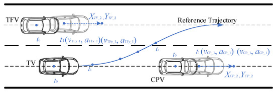
Figure 8.
Position prediction based on CA model.
4.4.2. Segmentation of Reference LC Trajectory
For the dynamic programming of LC trajectories, it essentially involves optimizing the reference trajectories Xref(t) and Yref(x). Leveraging real-time status information of adjacent vehicles (including position, velocity, and acceleration), the reference trajectories are dynamically optimized to derive the optimal LC trajectory. By dividing the reference trajectories into segments, optimization objective functions and constraints are established, and the objective functions of each segment are optimized to obtain the optimal trajectory.
Considering the limitation of onboard computing capabilities, the value should not be excessively large to avoid increasing the computational burden. However, if N is too small, the fitting effect of the trajectory curve will be subpar. In addition, LC durations are concentrated between 3 s and 10 s. After multiple simulation tests, the final option is N = 6, indicating an average duration of approximately 0.5 s to 1.6 s per segment, fulfilling the requirements for dynamic LC trajectory planning. Therefore, for the i-th segment of the LC trajectory:
For each trajectory segment Xref(t) and Yref(x), tli ≤ t ≤ tui, xli ≤ x ≤ xui, i = 1, 2, …, N. a0, …, a5i and b0, …, b5i are the coefficients of Xi(t) and Yi(x), tli and tui are the lower and upper boundary of the variable t for the i-th segment Xi(t), xli and xui are the lower and upper boundary of the variable x for the i-th segment Yi(x), and xli = Xi(tli), xui = Xi(tui).
4.4.3. Optimization Objective Function
The optimization objective of LC trajectories is to identify the point with the lowest risk field strength value and accomplish the LC in the smoothest manner with maximum efficiency, thereby avoiding prolonged disturbance to adjacent vehicles, while maintaining conformity with the reference trajectory curve as much as possible. Optimization is conducted individually for each segment of the LC trajectory. For the i-th segment trajectory, the optimization objective function is as follows:
where,
where w4, w5, …, w8, are the influencing coefficients, Disxi is the degree of conformity in the X direction between the i-th segment trajectory curve Xi(t) and the reference trajectory curve Xref(t), Dixyi is the degree of conformity in the Y direction between the i-th segment trajectory curve Yi(x) and the reference trajectory curve Yref(x), Ui is the risk field strength value of the i-th segment trajectory, feffi is the efficiency function, which is the ratio LC duration of the optimized trajectory to the duration of the reference trajectory, Jerkxi is the change rate of acceleration of the i-th segment; to maintain smoothness during LC, Jerkxi should be as small as possible.
Therefore, for the entire optimized LC trajectory, the overall optimization function is:
Optimizing and solving the y–x and x–t curves involve finding quintic polynomials Xi(t) and Yi(x) that minimize the optimization objective function Jsum under specific constraints.
4.4.4. Constraints Function
To ensure the feasibility of the LC trajectory curve after dynamic optimization, it is necessary to impose constraints on each segment of the polynomial curve to align with the vehicle’s driving requirements. These constraints encompass the starting and ending points of each polynomial segment, restrictions on the x–t curve and y–x curve, and smoothness criteria.
- (1)
- Constraints of Starting and Ending Points
For the optimized LC trajectory, its starting point is the starting point of the reference trajectories Xref(t) and Yref(x). The initial velocity, acceleration, and other states are identical to those of the starting points of Xref(t) and Yref(x). Therefore, the following constraints exist:
At the endpoint, the y-coordinate lies within the target lane, and both vy and ay are equal to 0. Therefore, the following constraints exist:
- (2)
- Constraints of x–t and y–x Curve
For the x–t curve, the lateral position should lie within the predicted feasible region. Furthermore, the first, second, and third derivatives of the x–t curve represent velocity, acceleration, and jerk, respectively, and must adhere to their upper and lower limit constraints.
In addition, for the y–x curve, the edge of TV should not exceed the boundary line. Moreover, the first, second, and third derivatives of the y–x curve represent arc length, curvature, and change rate of curvature, respectively, must adhere to the corresponding constraint conditions. Therefore, the following constraints are present:
Hence, the following constraints exist:
To ensure the safety, vmin = 0 m/s, vmax = 30 m/s, amin = −6 m/s2, amax = 4 m/s2, Jerkxmin = −2 m/s3, Jerkxmax = 2 m/s3, l is the arc length, ρ is the curvature of y–x curve, ensuring safety against sharp turns, and is the change rate of curvature, which is crucial for maintaining vehicle stability, especially during the LC process or sharp turns. Traverse all sampling points to determine the range of values, lmin = 0.2, lmax = 6.3, ρmin = 0.00002, ρmax = 0.0002, , .
- (3)
- Smoothness Constraints Condition
Additionally, the polynomial curves between segments should adhere to dynamical constraints, and nodes should possess continuity. That is, for the x–t curve and y–x curves, the motion state at the end of one segment should match the motion state at the beginning of the subsequent segment. Therefore, the following constraints must be fulfilled:
4.4.5. Dynamic Optimization Solution
In summary, the dynamic programming problem of LC trajectory can be viewed as a typical nonlinear optimization problem, aiming to find multiple polynomial segments Xi(t) and Yi(x) to optimize the objective function Jsum while satisfying a sequence of equality and inequality constraints to achieve the minimum value. The nonlinear optimization problem is reformulated into:
Equation (33) contains inequality constraints, which can be addressed by employing the penalty function method for the aforementioned nonlinear optimization problem. By applying the given constraints, an optimal LC trajectory can be computed.
5. Simulation Scenarios
The MATLAB 2023b simulation platform is utilized to validate the proposed dynamic LC trajectory planning algorithm. Four scenarios are set up: constant velocity, TFV decelerates, TFV accelerates and variable acceleration.
5.1. Simulation Scenario 1: Constant Velocity
The initial motion states of each vehicle in simulation scenario 1 are illustrated in Figure 9 and Table 3:

Figure 9.
Illustration of simulation scenarios 1, 2, and 3.

Table 3.
Initial motion states of each vehicle in simulation scenario 1.
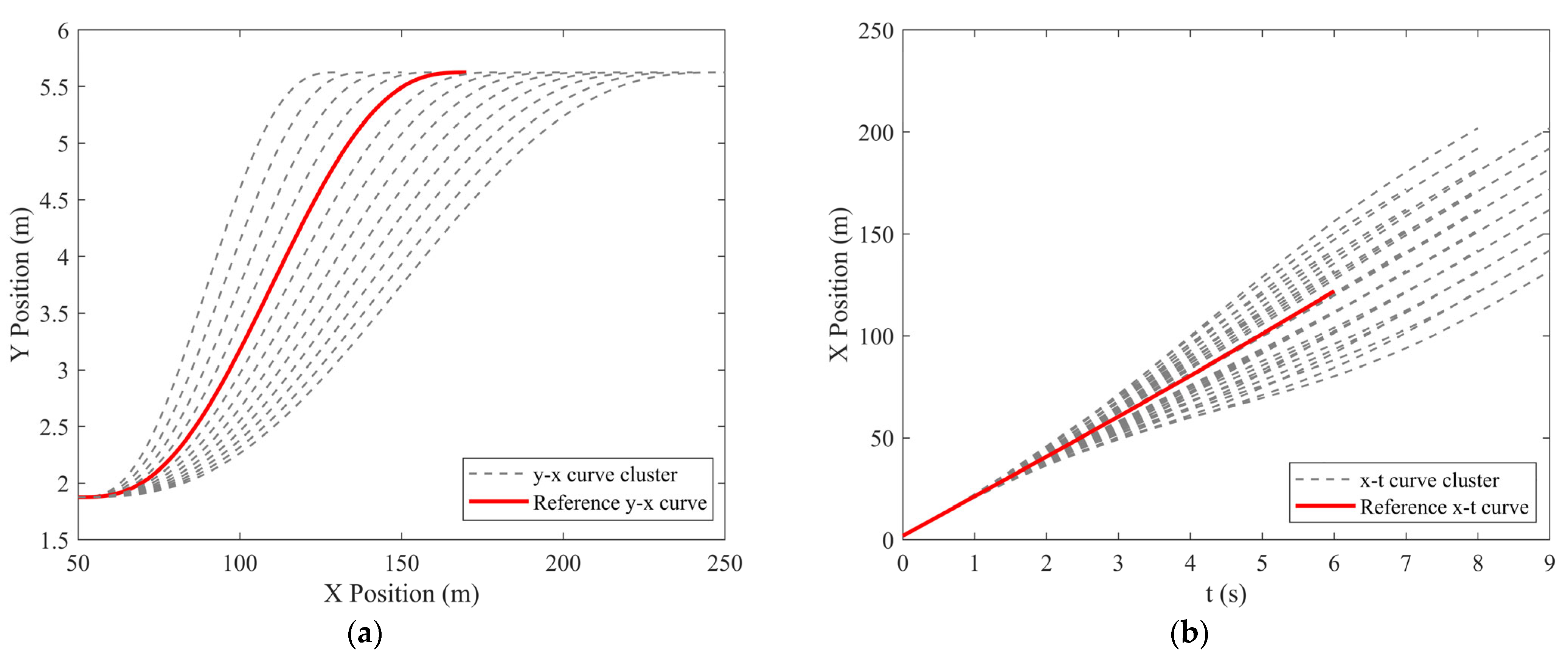
According to Section 4.2, after screening the LC trajectory cluster generated by quintic polynomial using constraints functions, an evaluation of the candidate trajectories that meet the constraints results in obtaining the reference trajectory, as shown in Figure 10.

Figure 10.
Reference LC trajectory selection results: (a) reference y–x curve and (b) reference x–t curve.
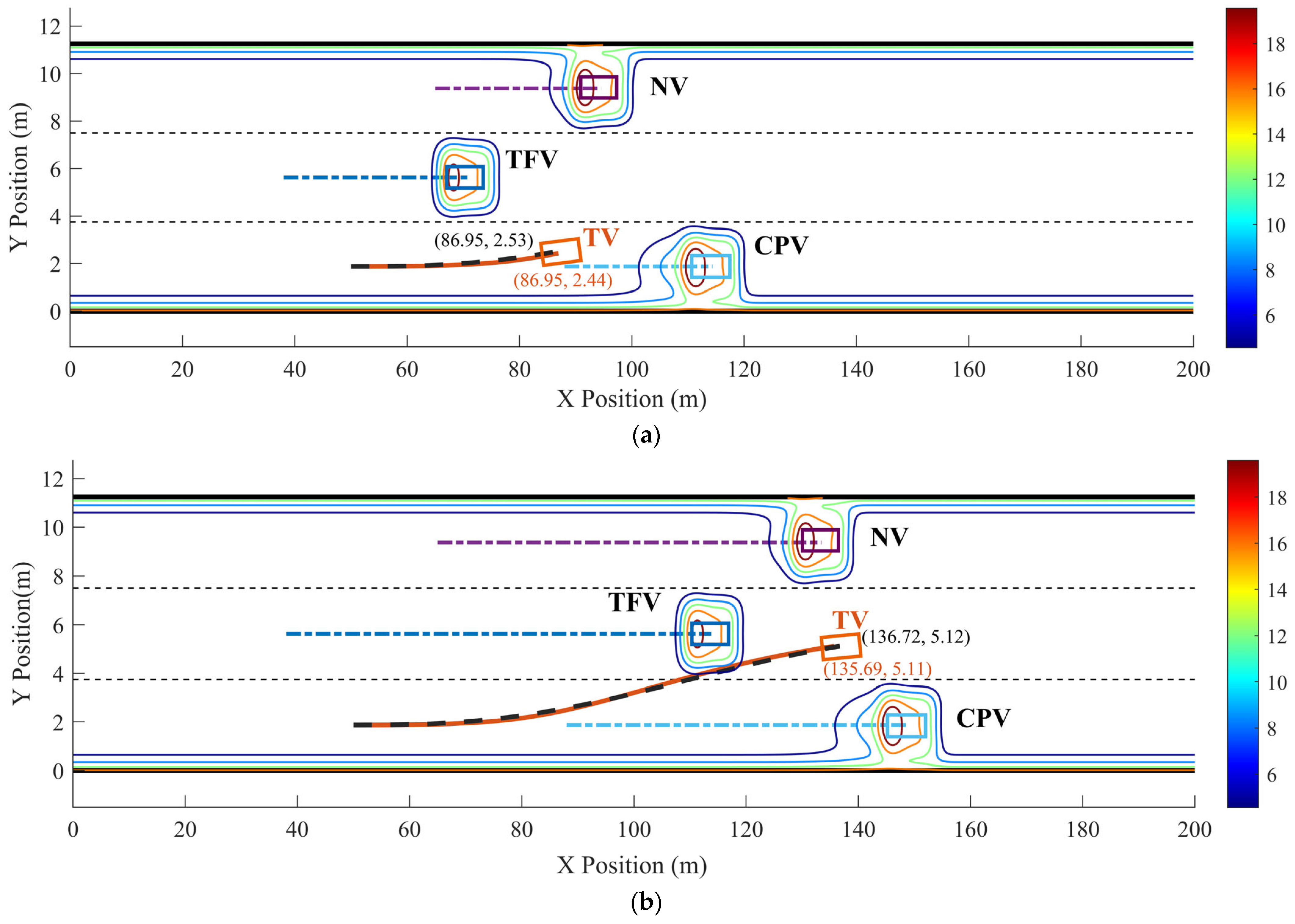
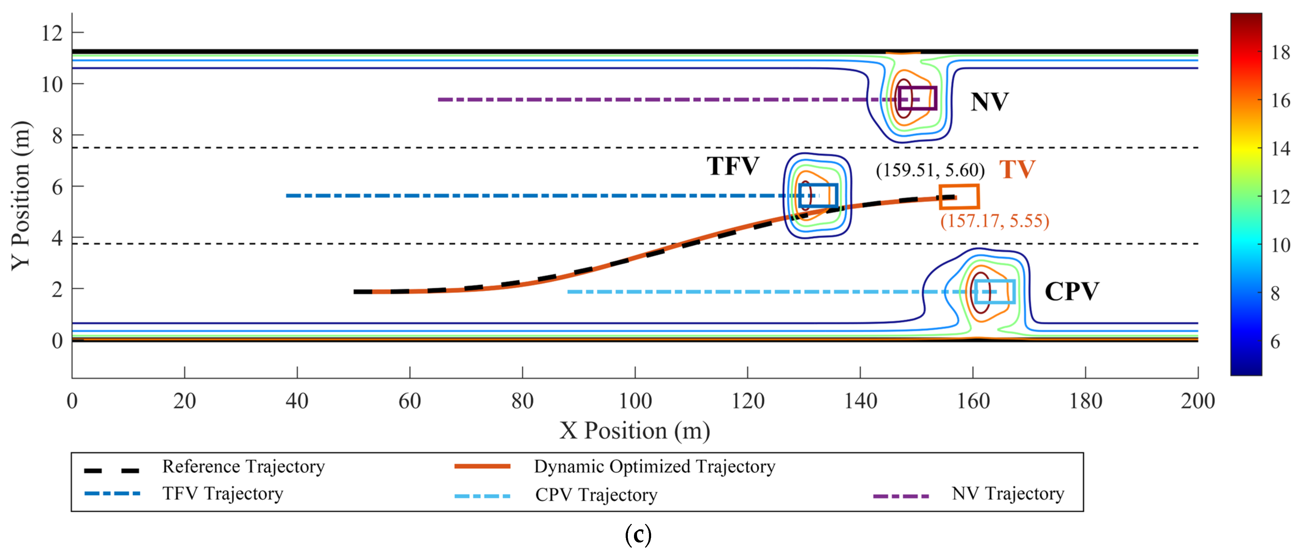
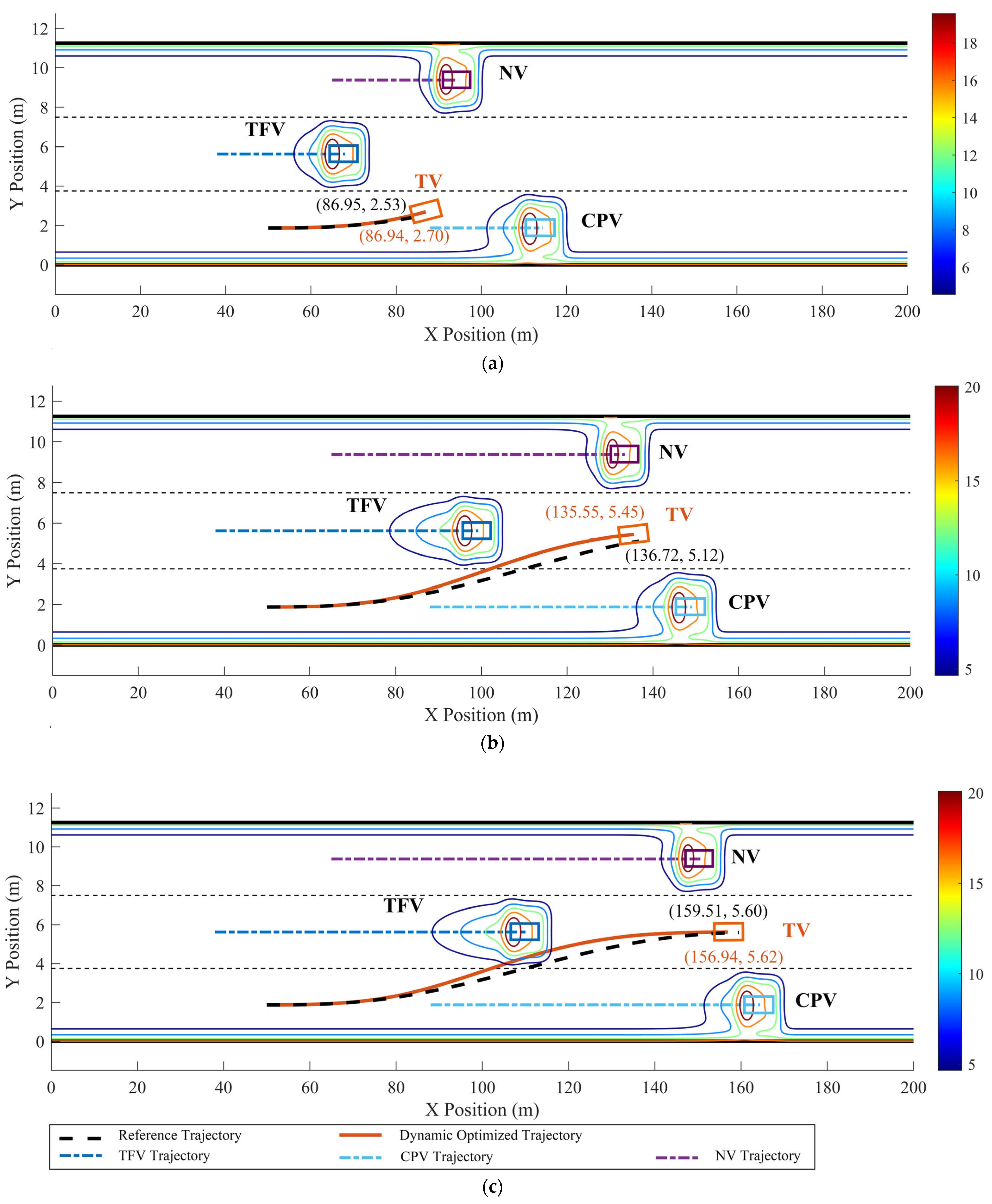
The optimized LC trajectory and motion state parameters are shown in Figure 11 and Figure 12. Figure 11 illustrates the reference trajectory and the optimized trajectory, overlaid with the real-time distribution of the MDRF.
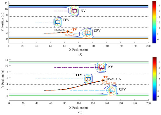
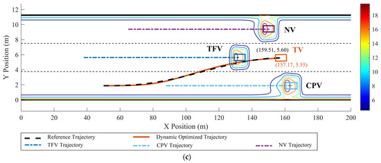
Figure 11.
Dynamic optimized LC trajectory planning result and MDRF distribution during the LC process in scenario 1: (a) t = 2 s, (b) t = 4.5 s, and (c) t = 5.6 s.
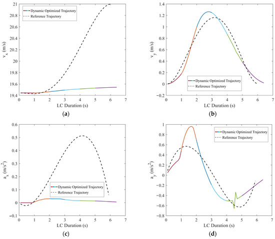
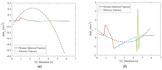
Figure 12.
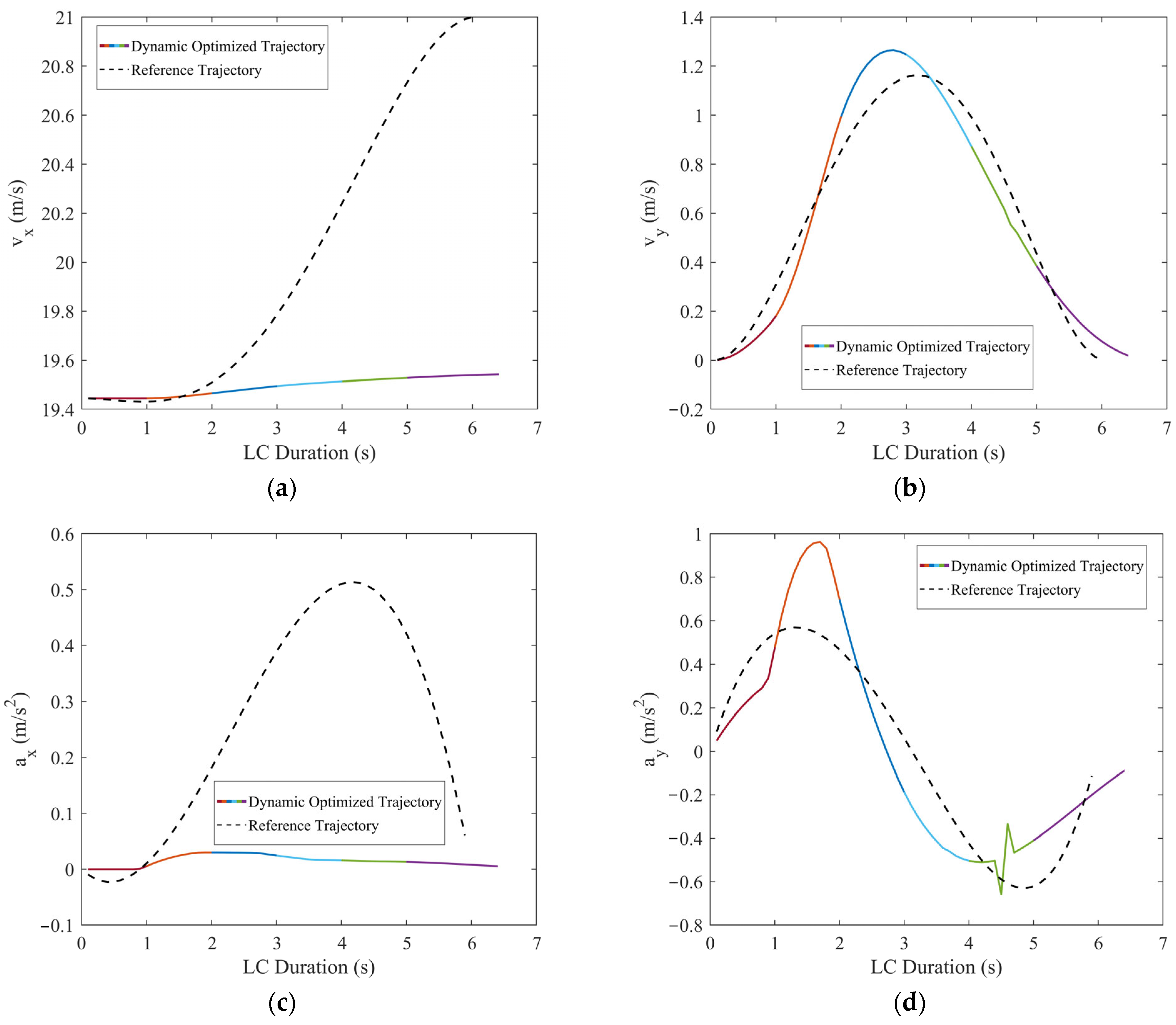
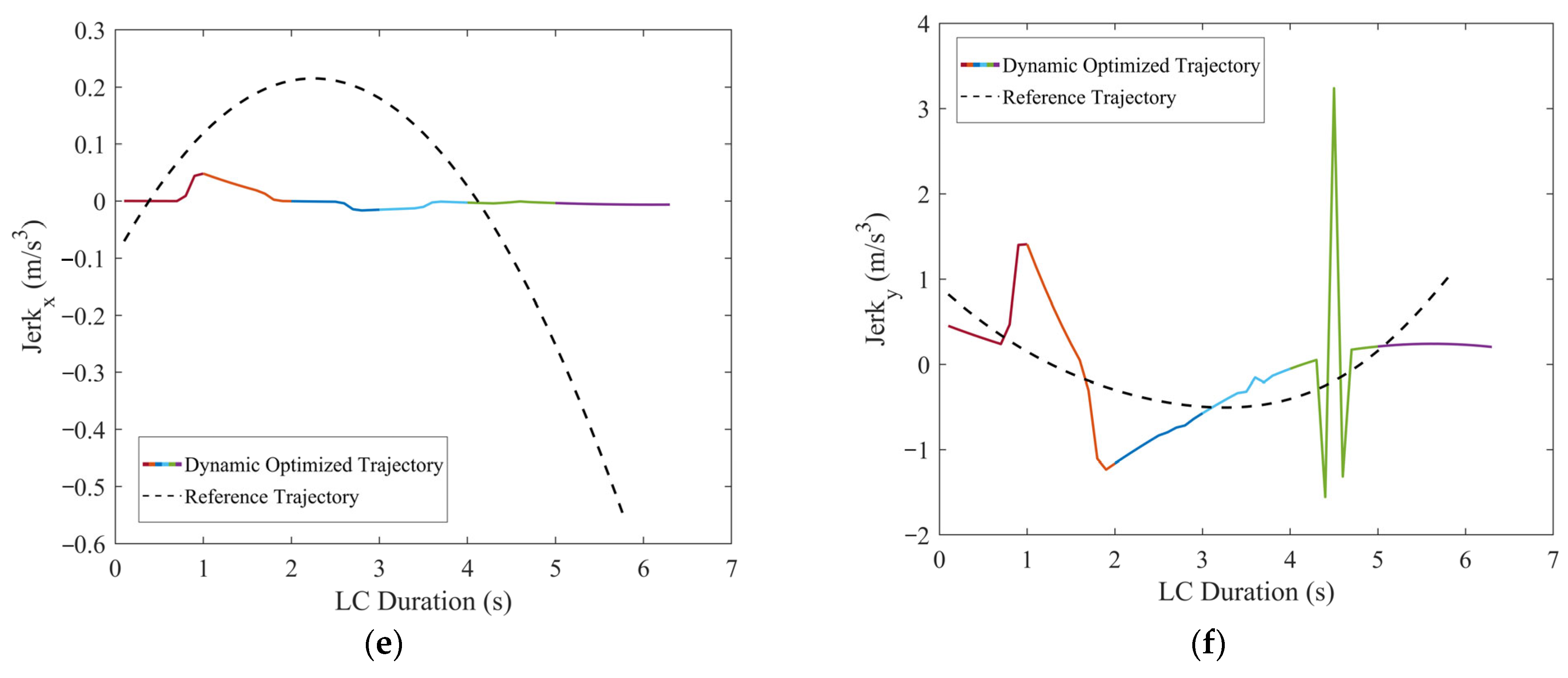
Comparisons of the motion parameters between dynamic optimized LC trajectory and reference LC trajectory for scenario 1: (a) Comparison of lateral velocities (vx); (b) comparison of longitudinal velocities (vy); (c) comparison of lateral accelerations (ax); (d) comparison of longitudinal accelerations (ay); (e) comparison of lateral jerk (Jerkx); and (f) comparison of longitudinal jerk (Jerky).
In scenario 1, each vehicle is moving at a constant velocity. It can be seen in Figure 11, when all vehicles are moving at a constant velocity, the optimized trajectory closely aligns with the reference trajectory. During the LC process, TV’s trajectory closely aligns with the point of minimum field strength, demonstrating the algorithm’s consideration for safety. From Figure 12, it is evident that the vx range of the optimized LC trajectory is between 19.44 m/s and 19.54 m/s, with very slight fluctuations in acceleration ax that fluctuate around 0, demonstrating excellent stability. vy ranges from 0 to 1.25 m/s, initially increasing and then decreasing, while ay ranges from −0.5 m/s2 to 1 m/s2. Additionally, both Jerkx and Jerky remain within the defined constraints. The changes in ax and ay, as well as Jerkx and Jerky, reflect the comfort and smoothness of the optimized trajectory. Moreover, each segment planned through programming ensures smooth transitions in path, velocity, acceleration, and jerk, ensuring smooth driving operations and passenger comfort, thus demonstrating the effectiveness and feasibility of the algorithm.
5.2. Simulation Scenario 2: TFV Decelerates
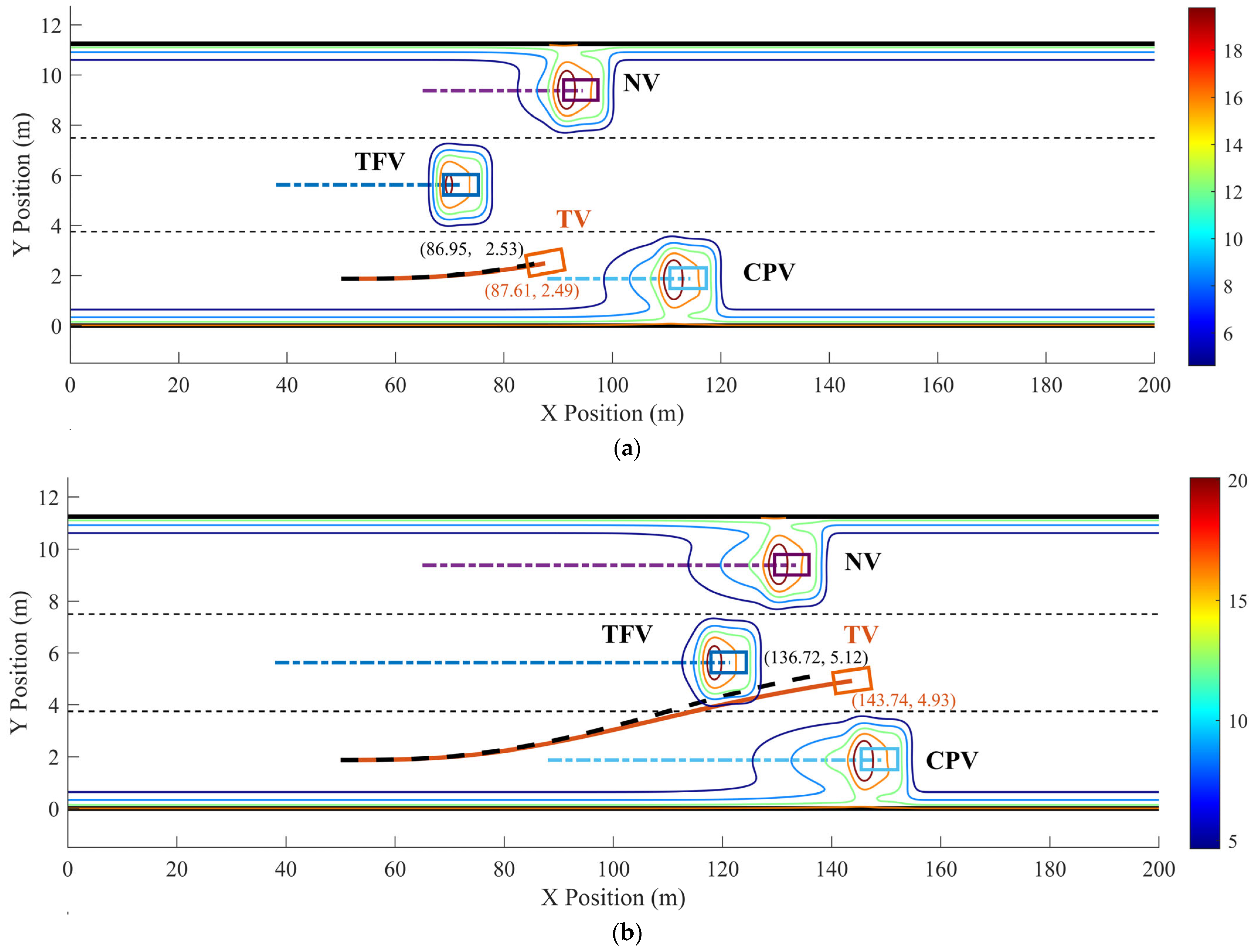
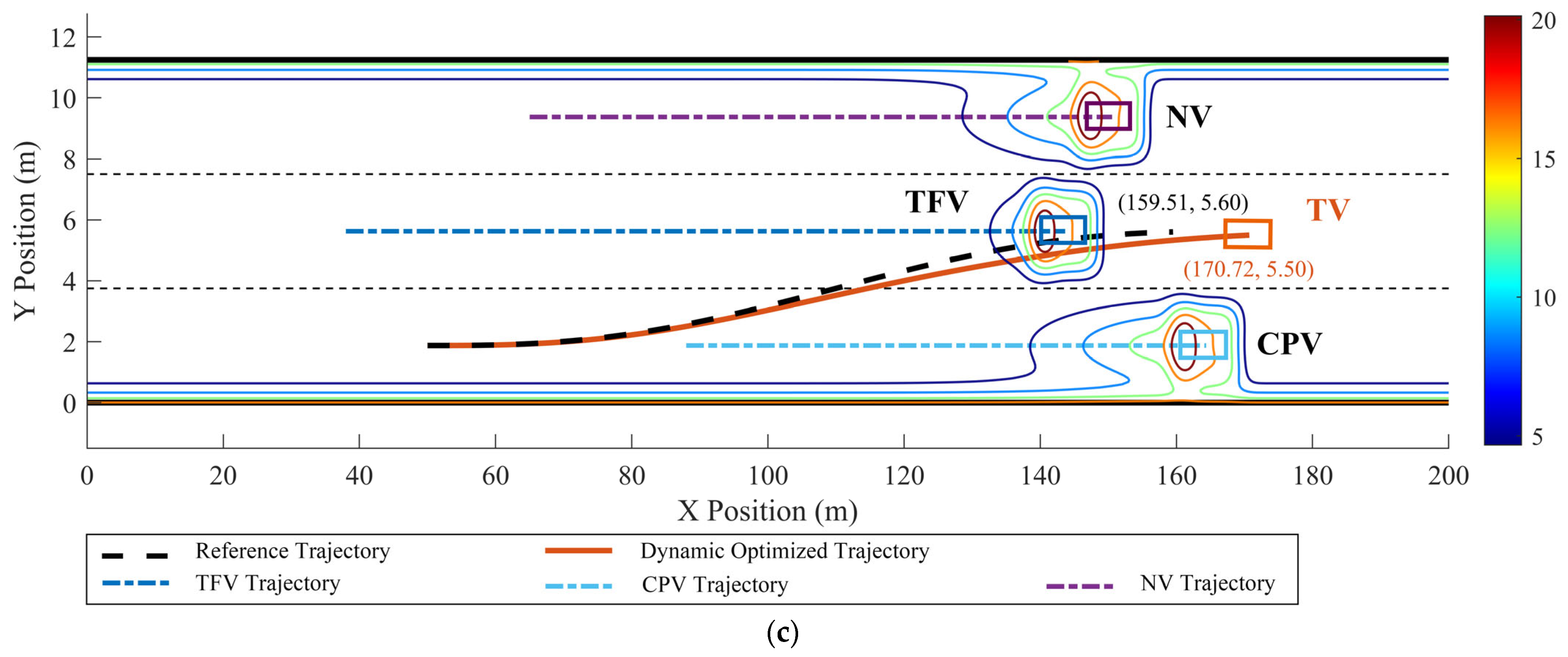
In scenario 2, apart from the TFV decelerating from 0~4 s with aTFV = −1.5 m/s2, the initial motion states of the other vehicles are identical to those in scenario 1, as shown in Figure 9.
The LC trajectory is dynamic optimized, and the optimal trajectory and motion state parameters are shown in Figure 13 and Figure 14. Since the initial states are the same as in scenario 1, the reference trajectory remains the same as in scenario 1.
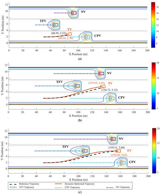
Figure 13.
Dynamic optimized LC trajectory planning result and MDRF distribution in scenario 2: (a) t = 2 s, (b) t = 4.5 s, and (c) t = 5.6 s.
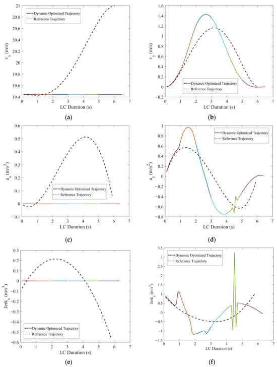
Figure 14.
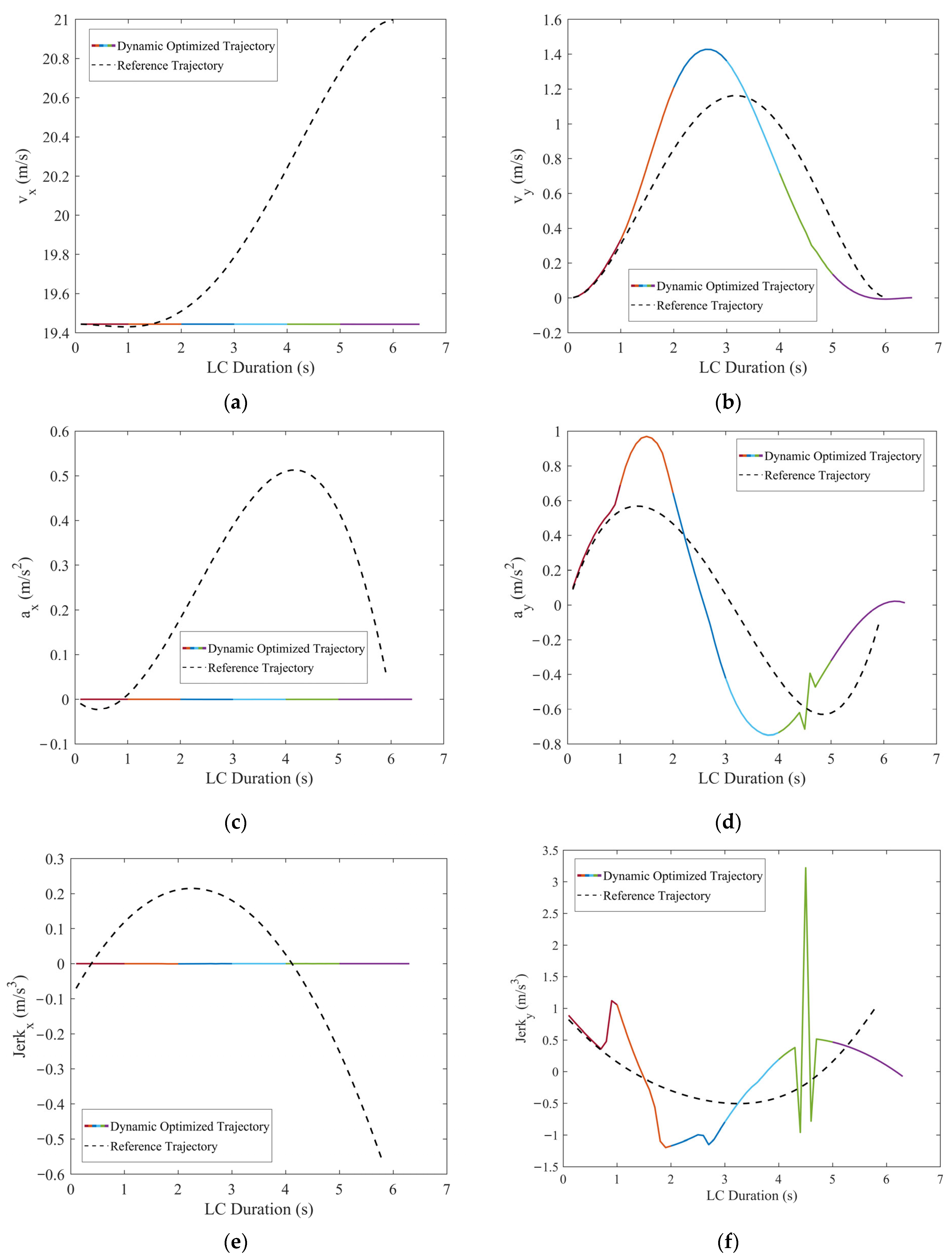
Comparisons of the motion parameters between dynamic optimized LC trajectory and reference LC trajectory for scenario 2: (a) Comparison of lateral velocities (vx); (b) comparison of longitudinal velocities (vy); (c) comparison of lateral accelerations (ax); (d) comparison of longitudinal accelerations (ay); (e) comparison of lateral jerk (Jerkx); and (f) comparison of longitudinal jerk (Jerky).
Figure 13 and Figure 14 show that, when TFV decelerates at aTFV = −1.5 m/s2, the optimized LC trajectory has undergone significant adjustments compared to the reference trajectory. Specifically, at t = 2 s, based on TFV’s real-time velocity and acceleration, the trajectory of TFV was promptly optimized and modified to predict its position at the next moment. Due to TFV being positioned further back laterally due to deceleration compared to its position during constant-speed motion, the optimized LC trajectory correspondingly shifted backward. As indicated in Figure 13, the x–t curve of the optimized trajectory completed the lane change approximately 3 m earlier compared to the reference trajectory. Furthermore, Figure 14a shows that TFV’s lateral velocity vx exhibited minimal variation, maintaining nearly constant speed with vx ≈ 19.44 m/s and the lateral acceleration ax ≈ 0. The longitudinal velocity vy ranged from 0~1.43 m/s, accelerating from 0~2.6 s, followed by smooth deceleration after 2.6 s, successfully entering the target lane.
5.3. Simulation Scenario 3: TFV Accelerates
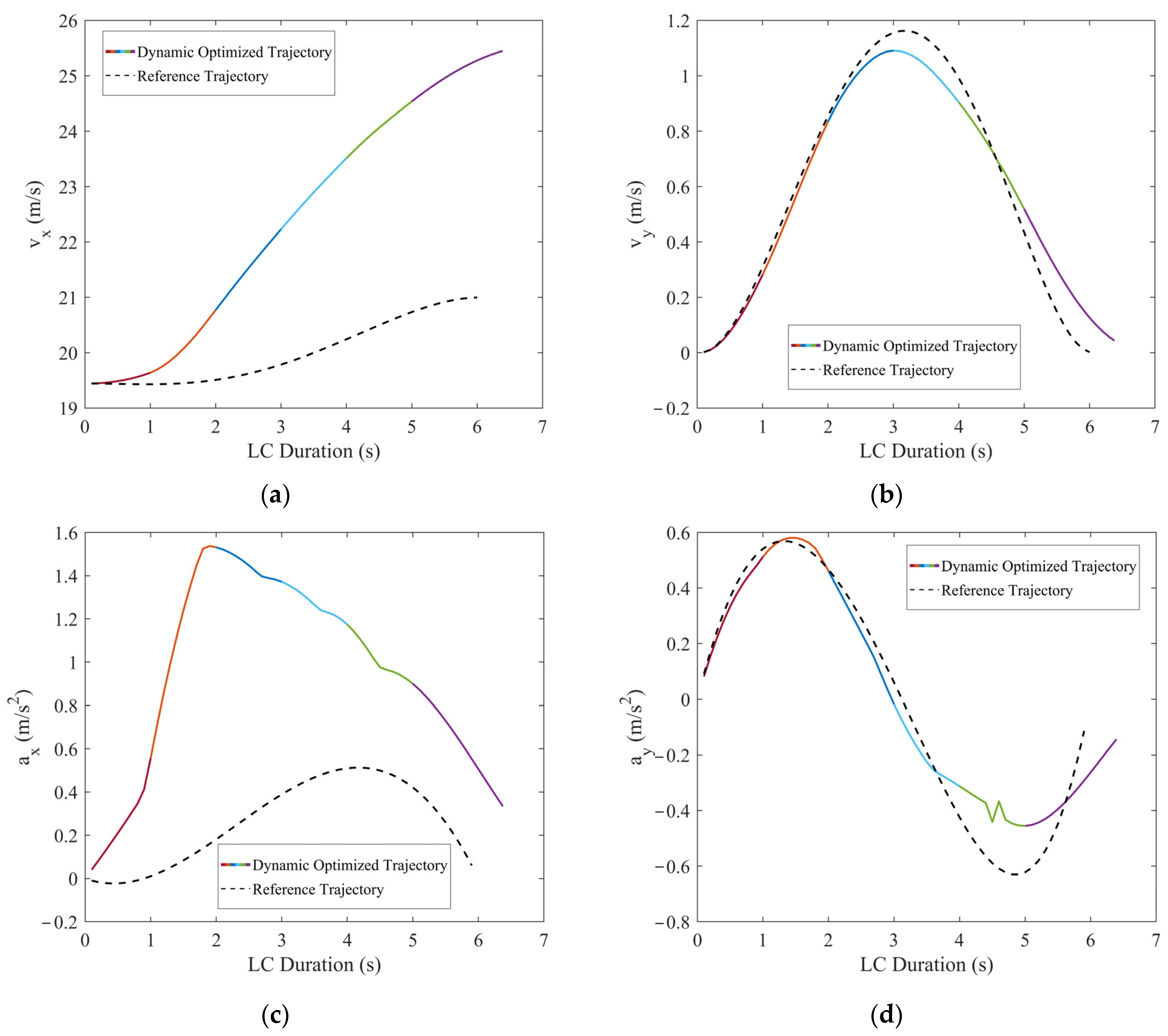
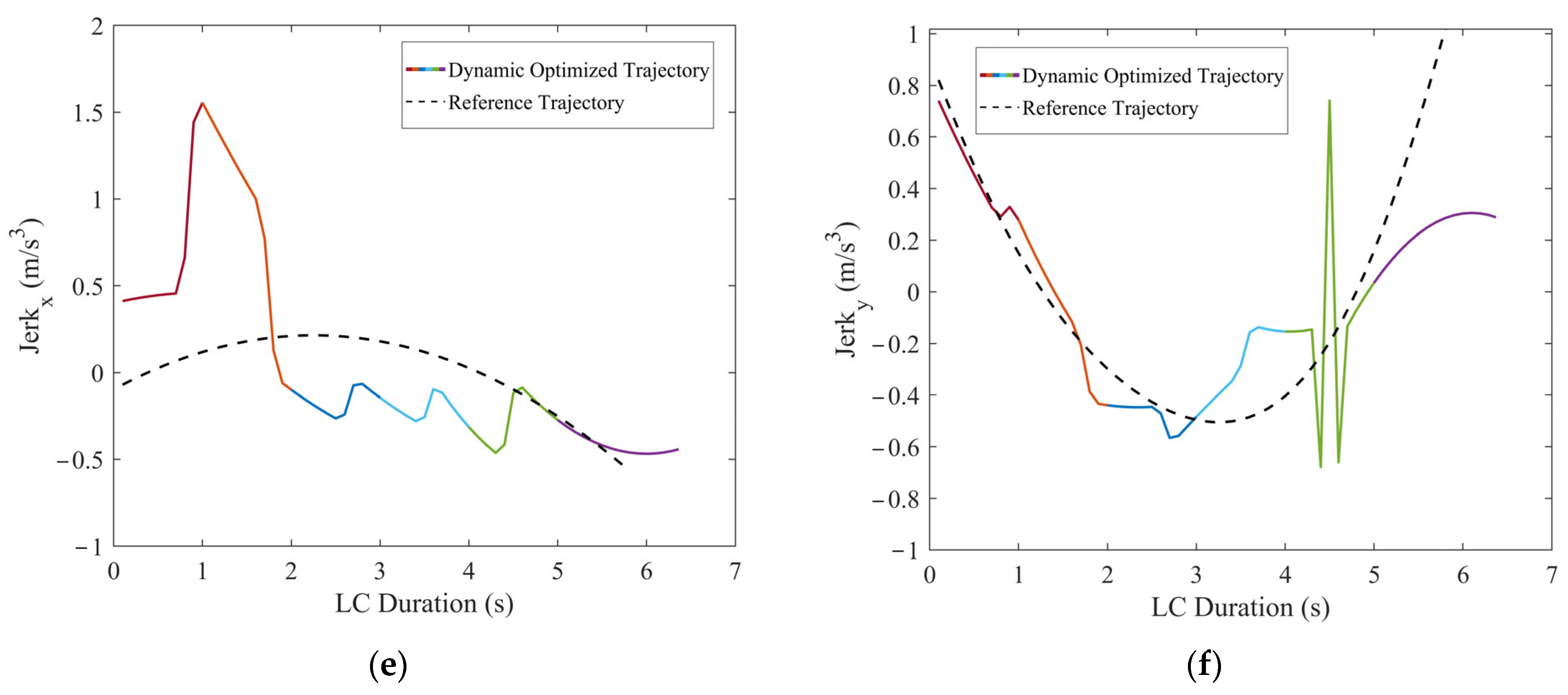
In scenario 3, apart from the TFV accelerating from 0~4 s with aTFV = 0.8 m/s2, the initial motion states of the other vehicles are identical to those in scenario 1, as shown in Figure 9. The optimized LC trajectory and motion state parameters are depicted in Figure 15 and Figure 16.
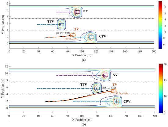
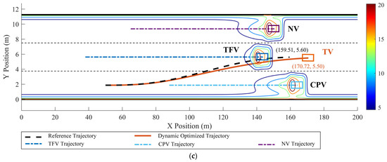
Figure 15.
Dynamic optimized LC trajectory planning result and MDRF distribution in scenario 3: (a) t = 2 s, (b) t = 4.5 s, and (c) t = 5.6 s.
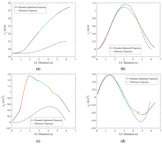

Figure 16.
Comparisons of the motion parameters between dynamic optimized LC trajectory and reference LC trajectory for scenario 3: (a) Comparison of lateral velocities (vx); (b) comparison of longitudinal velocities (vy); (c) comparison of lateral accelerations (ax); (d) comparison of longitudinal accelerations (ay); (e) comparison of lateral jerk (Jerkx); and (f) comparison of longitudinal jerk (Jerky).
In Figure 15 and Figure 16, when TFV accelerates with a = 0.8 m/s2, it can be observed that the dynamic optimized LC trajectory has been significantly adjusted compared to the reference trajectory. Relative to the reference trajectory, the optimized x–t curve is adjusted forward within a range of approximately 0~15 m and the y–x curve is adjusted within approximately 0~0.4 m. Compared to the reference trajectory, the optimized x–t curve completes the LC approximately 11 m later. The risk field distribution in Figure 15 shows that the risk associated with the optimized trajectory is significantly lower than that of the reference trajectory, indicating the effectiveness of the method in risk avoidance. According to Figure 16, TV’s lateral velocity vx varies significantly, accelerating from 19.44 m/s to 25.6 m/s during the LC process, with an acceleration of 0 < ax < 1.53 m/s2, indicating that TV aimed to speed up to quickly move away from TFV and increase the safety distance. The longitudinal velocity vy ranges from 0~1.1 m/s, initially accelerating from 0~2.9 s with an acceleration of 0 < ay < 0.58 m/s2, and then decelerating after 2.9 s with −0.45 m/s2 < ay < 0, signifying TV enters the target lane after 2.9 s.
5.4. Simulation Scenario 4: Variable Acceleration
In order to validate the scenario involving variable acceleration, scenario 4 is configured as depicted in Figure 17 and Table 4.

Figure 17.
Reference LC trajectory selection results.

Table 4.
Initial motion states of each vehicle in simulation scenario 4.
The LC trajectory of scenario 4 is optimized, and the optimized trajectory and motion state parameters are shown in Figure 18 and Figure 19.
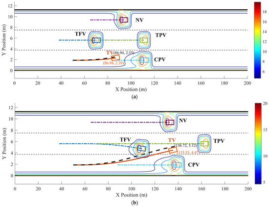
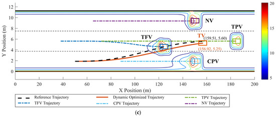
Figure 18.
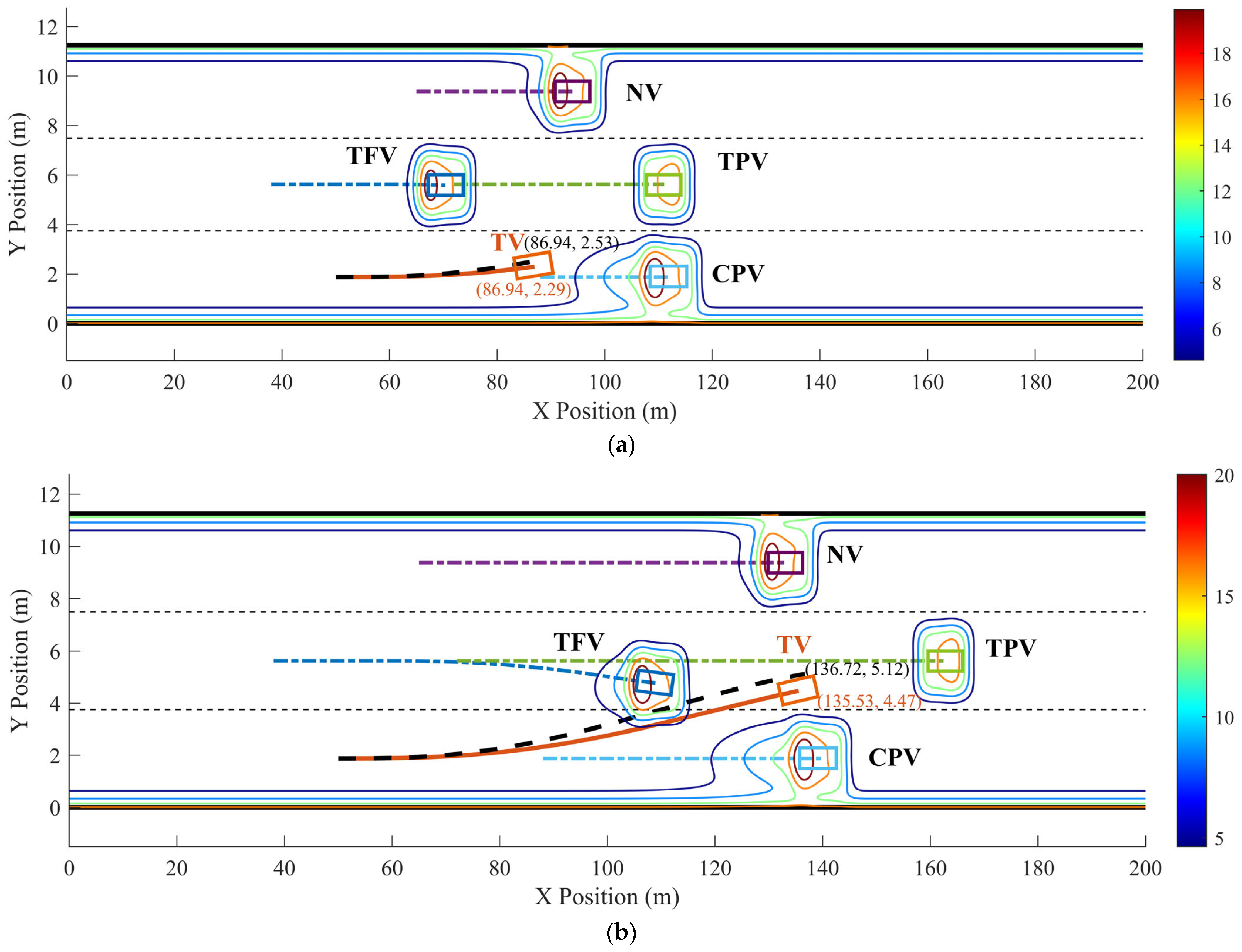
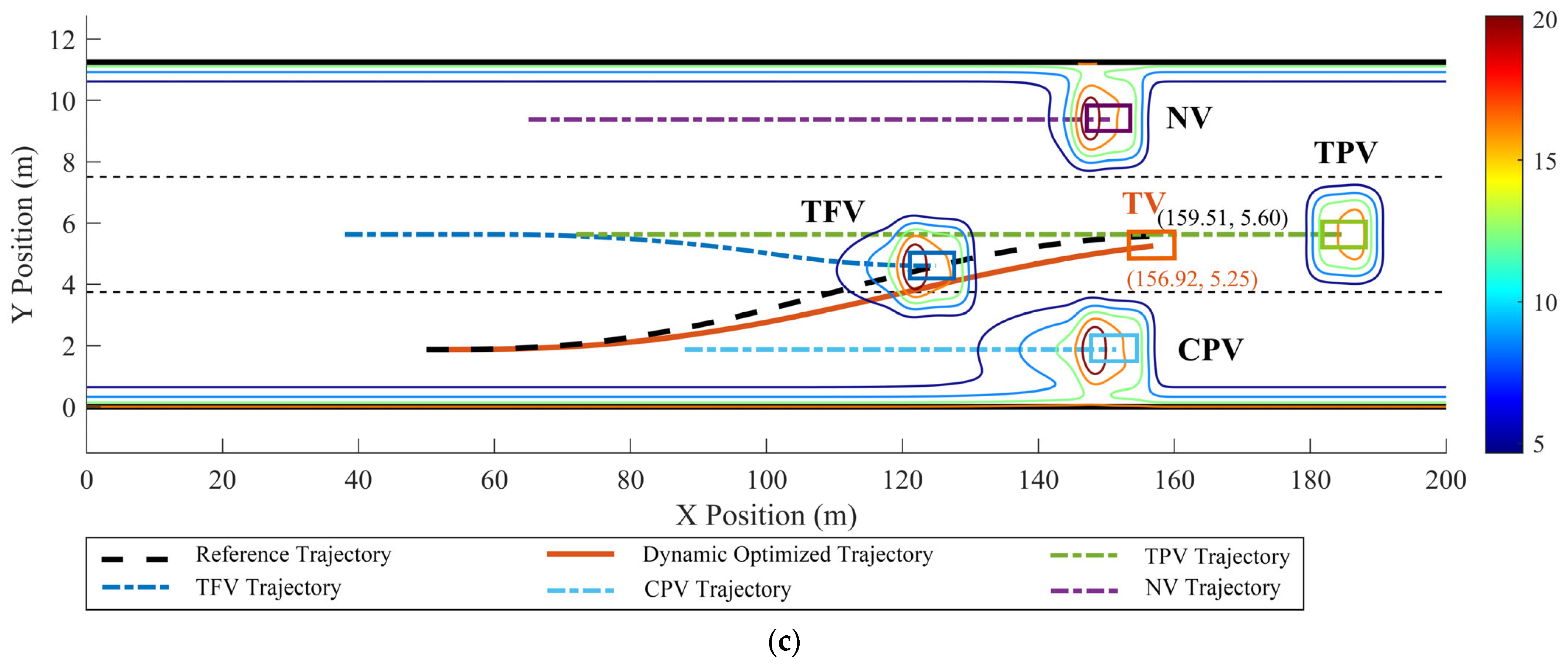
Dynamic optimized LC trajectory planning result and MDRF distribution in scenario 4: (a) t = 2 s, (b) t = 4.5 s, and (c) t = 5.6 s.
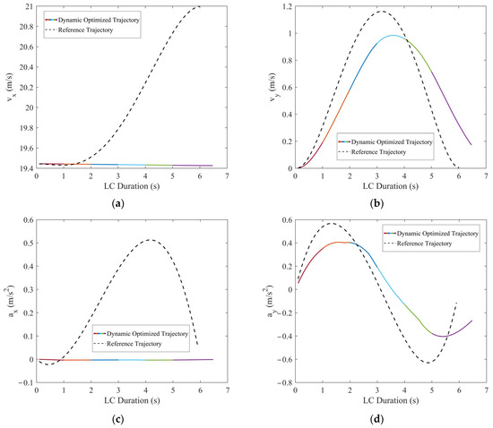
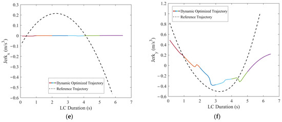
Figure 19.
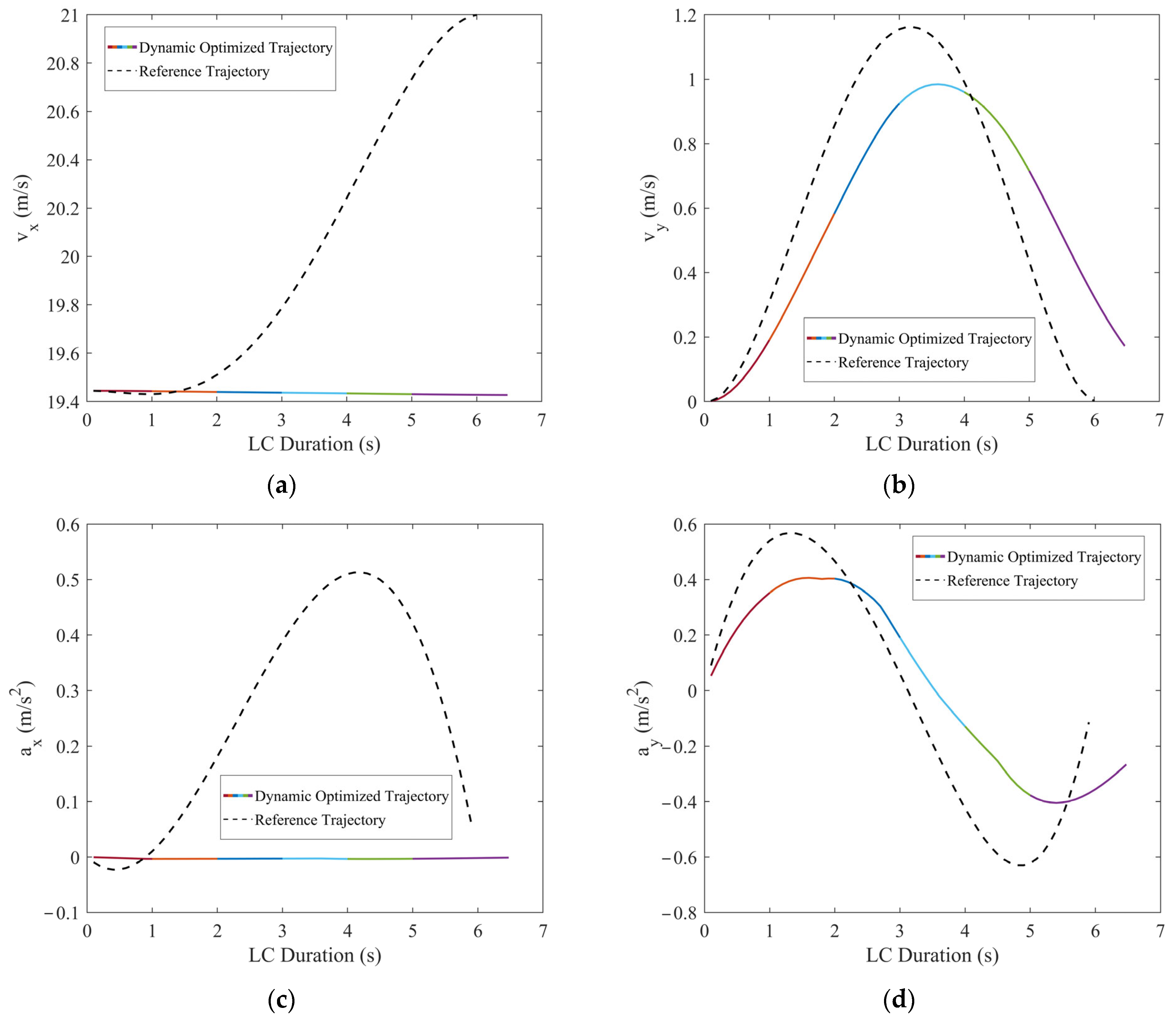
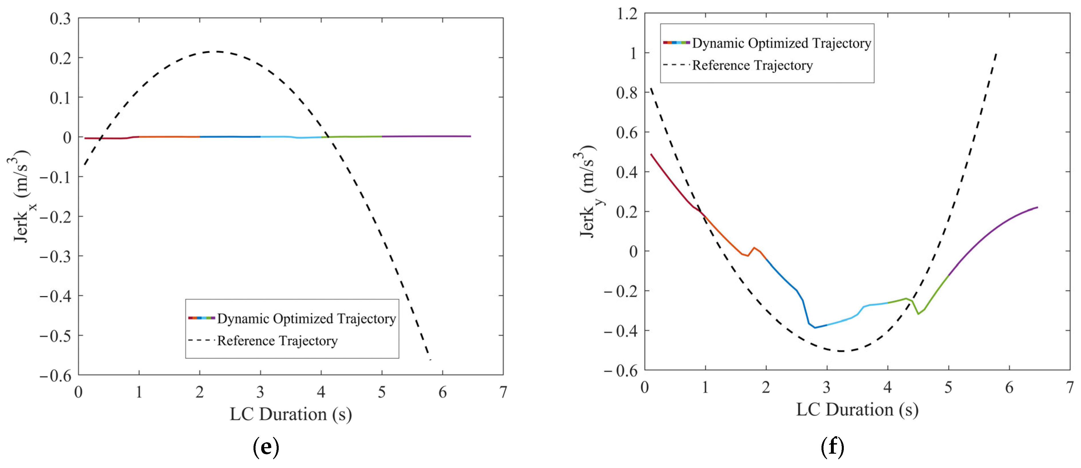
Comparisons of the motion parameters between dynamic optimized LC trajectory and reference LC trajectory for scenario 4: (a) Comparison of lateral velocities (vx); (b) comparison of longitudinal velocities (vy); (c) comparison of lateral accelerations (ax); (d) comparison of longitudinal accelerations (ay); (e) comparison of lateral jerk (Jerkx); and (f) comparison of longitudinal jerk (Jerky).
In scenario 4, the TFV and CPV exhibit variable acceleration patterns while considering the presence of TPV. Combining Figure 18 and Figure 19, the optimized LC trajectory has been significantly modified in comparison to the reference trajectory. Specifically, at t = 1 s, aTFV,x = −0.7 m/s2, aTFV,y = −0.2 m/s2, aCFV = −1.1 m/s2. At this point, as both TFV and CPV have initiated deceleration, TV promptly adjusts its trajectory in a timely manner based on the real-time velocity and acceleration of TFV and CPV. After predicting the positions of TFV and CPV for the next moment, TV’s trajectory is optimized accordingly. Influence by aTFV,y, TFV begins to approach TV in the Y direction. Consequently, the position of TV in the Y direction starts to shift downward compared to the reference trajectory. The maximum downward offset of the optimized trajectory on the y–x curve is approximately 0.6 m. During the interval [4 s, 6 s], with aTFV,x = −1.0 m/s2, aTFV,y = 0.32 m/s2, TFV starts moving away from TV in the Y direction. Compared to the previous segment, the optimized trajectory in this segment exhibits a reduced downward offset in the Y direction. At this point, the downward offset of the optimized trajectory on the y–x curve is approximately 0.4 m. Moreover, the distribution of the risk field in Figure 18 indicates that the risk associated with the optimized trajectory is significantly reduced compared to the reference trajectory. As indicated in Figure 19, TV’s lateral velocity vx remains relatively constant with vx ≈ 19.44 m/s, ax ≈ 0. The longitudinal velocity vy ranges between 0 and 0.98 m/s, accelerating initially within the interval [0, 3.6 s], then decelerating after 3.6 s, indicating TV successfully enters the target lane after 3.6 s.
Furthermore, the runtime performance of the scenarios 1~4 are as follows (Table 5):

Table 5.
Runtime performance of the scenarios 1~4.
These runtimes are well within the acceptable range for real-time applications, as they allow for sufficient time to process sensor data, perform trajectory planning, and execute control commands during an LC process. Moreover, the runtime of the simulation increases with the complexity of the scenarios, which is consistent with real-world conditions. The simulations were conducted on a platform using MATLAB 2023b, and the hardware configuration used for the simulations includes a system with 8 GB of RAM and an NVIDIA GeForce GTX 1650 GPU. This setup is representative of mid-range computational capabilities, indicating that the algorithms are feasible for implementation in ICVs with similar or higher computational resources.
In conclusion, the four simulation scenarios obtained smooth and continuous LC trajectory curves. The variations in velocity, acceleration, and jerk all comply with vehicle dynamics and conditional constraints. Moreover, the TVs are capable of dynamically adjusting their trajectories in real time based on the instantaneous states of adjacent vehicles, meeting the safety requirements of the MDRF function, thus effectively enhancing driving safety. Specifically, while TV is in the current lane, based on the adjacent vehicles’ real-time velocity and acceleration, the predicted position at the next moment is obtained, and the trajectory of TV is timely adjusted and optimized. In addition, the computational complexity of the proposed algorithms is sufficiently low to meet the stringent real-time requirements of ICVs. Consequently, the LC trajectory dynamic planning algorithm proposed in this study demonstrates high adaptability and practicality, enabling safe, smooth, and comfortable LC maneuvers in various LC scenarios.
6. Conclusions
This study presents a dynamic LC trajectory planning algorithm for ICVs, leveraging a multi-vehicle MDRF model. As validated through simulations, the algorithm ensures safe and comfortable LC maneuvers in dynamic traffic environments. The MDRF model, grounded on APF theory, evaluates environmental risk by integrating the kinematic and geometric attributes of adjacent vehicles, providing a theoretical foundation for LC trajectory planning.
By decomposing trajectory planning into path planning and velocity planning, this paper employs the path-velocity decomposition approach to reduce the dimensionality of trajectory planning. Constrained criteria are then added to the LC trajectory clusters, eliminating trajectories that do not meet the requirements of vehicle dynamics and safety. Compared to traditional trajectory planning methods, this approach reduces computational power consumption and enhances algorithm efficiency.
Based on the reference trajectories Xref(t) and Yref(x), the LC trajectory is segmented for dynamic planning. Utilizing the MDRF model, a multi-objective optimization function is constructed, incorporating constraints including continuity, kinematic feasibility, and smoothness. By applying the penalty function method to solve the optimization objective function, the optimal LC trajectory is determined. According to the simulation results, the dynamic LC trajectory planning algorithm based on the MDRF model proposed in this paper demonstrates better smoothness and comfort while maintaining the continuity and dynamic feasibility of the LC trajectory in various complex LC scenarios. Additionally, it exhibits remarkable safety and adaptability when confronted with intricate, dynamic LC scenarios. In conclusion, this study contributes an approach to LC trajectory planning that addresses the challenges of dynamic traffic conditions, showing the potential for practical implementation in ICV systems.
Future work will integrate human decision-making data from real-world scenarios to enhance predictive algorithms. Advanced sensor fusion using sophisticated sensors will improve perceptual capabilities and robustness. Furthermore, real traffic data will ground algorithms in practical, complex conditions, fostering a deeper understanding of vehicular interactions and environmental dynamics. Collectively, these efforts aim to refine trajectory planning algorithms, enabling effective decision-making for diverse road conditions and advancing the robustness of next-generation ICVs.
Author Contributions
Conceptualization, L.Z. and W.L.; methodology, L.Z.; software, L.Z.; validation, L.Z.; formal analysis, L.Z.; investigation, L.Z. and C.Z.; resources, L.Z.; data curation, L.Z.; writing original draft preparation, L.Z.; writing review and editing, L.Z.; visualization, L.Z. and C.Z.; supervision, W.L.; project administration, W.L.; funding acquisition, W.L and C.Z. All authors have read and agreed to the published version of the manuscript.
Funding
This research was funded by Natural Science Foundation of Guangdong Province: 2024A1515012376, 2022A1515010948.
Data Availability Statement
Data are contained within the article.
Conflicts of Interest
The authors declare no conflicts of interest.
References
- Zhai, C.; Li, K.; Zhang, R.; Peng, T.; Zong, C. Phase Diagram in Multi-Phase Heterogeneous Traffic Flow Model Integrating the Perceptual Range Difference under Human-Driven and Connected Vehicles Environment. Chaos Solitons Fractals 2024, 182, 114791. [Google Scholar] [CrossRef]
- Zhai, C.; Wu, W.; Xiao, Y. The Jamming Transition of Multi-Lane Lattice Hydrodynamic Model with Passing Effect. Chaos Solitons Fractals 2023, 171, 113515. [Google Scholar] [CrossRef]
- Makridis, M.; Leclercq, L.; Ciuffo, B.; Fontaras, G.; Mattas, K. Formalizing the Heterogeneity of the Vehicle-Driver System to Reproduce Traffic Oscillations. Transp. Res. Part C Emerg. Technol. 2020, 120, 102803. [Google Scholar] [CrossRef]
- Knoop, V.L.; Hoogendoorn, S.P.; Shiomi, Y.; Buisson, C. Quantifying the Number of Lane Changes in Traffic: Empirical Analysis. Transp. Res. Rec. 2012, 2278, 31–41. [Google Scholar] [CrossRef]
- Zhang, R.; Zhong, W.; Wang, N.; Sheng, R.; Wang, Y.; Zhou, Y. The Innovation Effect of Intelligent Connected Vehicle Policies in China. IEEE Access 2022, 10, 24738–24748. [Google Scholar] [CrossRef]
- Zeng, J.; Qian, Y.; Li, J.; Zhang, Y.; Xu, D. Congestion and Energy Consumption of Heterogeneous Traffic Flow Mixed with Intelligent Connected Vehicles and Platoons. Phys. A Stat. Mech. Its Appl. 2023, 609, 128331. [Google Scholar] [CrossRef]
- Ning, H.; Yin, R.; Ullah, A.; Shi, F. A Survey on Hybrid Human-Artificial Intelligence for Autonomous Driving. IEEE Trans. Intell. Transport. Syst. 2022, 23, 6011–6026. [Google Scholar] [CrossRef]
- ISO/SAE PAS 22736; Taxonomy and Definitions for Terms Related to Driving Automation Systems for On-Road Motor Vehicles. ISO: Geneva, Switzerland, 2021.
- Manjunath, R.; Saddaladinne, J.B.; Gopinath, D. Enhancing Safety Features of Advanced Driver Assistance System Warnings by Using Head-up Displays. In Proceedings of the WCX SAE World Congress Experience, Detroit, MI, USA, 18–20 April 2024; SAE International: Warrendale, PA, USA, 2024. [Google Scholar]
- Noonan, T.Z.; Gershon, P.; Mehler, B.; Reimer, B. Characterizing the Use of Tesla’s Auto Lane Change Feature in Driver-Initiated Maneuvers. Proc. Hum. Factors Ergon. Soc. Annu. Meet. 2022, 66, 1442–1446. [Google Scholar] [CrossRef]
- Mueller, A.S.; Cicchino, J.B.; Calvanelli, J.V., Jr. Consumer Demand for Partial Driving Automation and Hands-Free Driving Capability. J. Saf. Res. 2023, 84, 371–383. [Google Scholar] [CrossRef]
- NHTSA. Summary Report: Standing General Order on Crash Reporting for Level 2 Advanced Driver Assistance Systems; National Highway Traffic Safety Administration: Washington, DC, USA, 2023. [Google Scholar]
- Khan, M.A. Intelligent Environment Enabling Autonomous Driving. IEEE Access 2021, 9, 32997–33017. [Google Scholar] [CrossRef]
- Ma, Y.; Dong, F.; Yin, B.; Lou, Y. Real-Time Risk Assessment Model for Multi-Vehicle Interaction of Connected and Autonomous Vehicles in Weaving Area Based on Risk Potential Field. Phys. A Stat. Mech. Its Appl. 2023, 620, 128725. [Google Scholar] [CrossRef]
- Briz-Redón, Á.; Martínez-Ruiz, F.; Montes, F. Identification of Differential Risk Hotspots for Collision and Vehicle Type in a Directed Linear Network. Accid. Anal. Prev. 2019, 132, 105278. [Google Scholar] [CrossRef] [PubMed]
- Wang, J.; Wu, J.; Zheng, X.; Ni, D.; Li, K. Driving Safety Field Theory Modeling and Its Application in Pre-Collision Warning System. Transp. Res. Part C Emerg. Technol. 2016, 72, 306–324. [Google Scholar] [CrossRef]
- Martínez, C.; Jiménez, F. Implementation of a Potential Field-Based Decision-Making Algorithm on Autonomous Vehicles for Driving in Complex Environments. Sensors 2019, 19, 3318. [Google Scholar] [CrossRef]
- Liu, P.; Jia, H.; Zhang, L.; Wang, Z. Lane-Changing Trajectory Planning for Autonomous Vehicles on Structured Roads. J. Mech. Eng. 2023, 59, 271–281. [Google Scholar]
- Wang, M.; Zhang, L.; Zhang, Z.; Wang, Z. A Hybrid Trajectory Planning Strategy for Intelligent Vehicles in On-Road Dynamic Scenarios. IEEE Trans. Veh. Technol. 2023, 72, 2832–2847. [Google Scholar] [CrossRef]
- Sun, B.; Ma, G.; Song, J.; Cheng, Z.; Wang, W. Driving Safety Field Modeling Focused on Heterogeneous Traffic Flows and Cooperative Control Strategy in Highway Merging Zone. Phys. A Stat. Mech. Its Appl. 2023, 630, 129215. [Google Scholar] [CrossRef]
- Tian, Y.; Pei, H.; Yang, J.; Hu, J.; Zhang, Y.; Pei, X. An Improved Model of Driving Risk Field for Connected and Automated Vehicles. In Proceedings of the 2021 IEEE International Intelligent Transportation Systems Conference (ITSC), Indianapolis, IN, USA, 19–22 September 2021; IEEE: Piscataway, NJ, USA, 2021; pp. 285–291. [Google Scholar]
- Li, L.; Gan, J.; Zhou, K.; Qu, X.; Ran, B. A Novel Lane-Changing Model of Connected and Automated Vehicles: Using the Safety Potential Field Theory. Phys. A Stat. Mech. Its Appl. 2020, 559, 125039. [Google Scholar] [CrossRef]
- Mullakkal-Babu, F.A.; Wang, M.; He, X.; Van Arem, B.; Happee, R. Probabilistic Field Approach for Motorway Driving Risk Assessment. Transp. Res. Part C Emerg. Technol. 2020, 118, 102716. [Google Scholar] [CrossRef]
- Chen, T.; Shi, X.; Wong, Y.D. A Lane-Changing Risk Profile Analysis Method Based on Time-Series Clustering. Phys. A Stat. Mech. Its Appl. 2021, 565, 125567. [Google Scholar] [CrossRef]
- Li, L.; Gan, J.; Ji, X.; Qu, X.; Ran, B. Dynamic Driving Risk Potential Field Model Under the Connected and Automated Vehicles Environment and Its Application in Car-Following Modeling. IEEE Trans. Intell. Transport. Syst. 2022, 23, 122–141. [Google Scholar] [CrossRef]
- Son, Y.S.; Kim, W. Cooperation-Based Risk Assessment Prediction for Rear-End Collision Avoidance in Autonomous Lane Change Maneuvers. Actuators 2022, 11, 98. [Google Scholar] [CrossRef]
- Zhang, Y.; Shuai, B.; Zhang, R.; Fan, C.; Huang, W. Modeling and Simulation of Driving Risk Pulse Field and Its Application in Car Following Model. IEEE Trans. Intell. Transp. Syst. 2024, 25, 8984–9000. [Google Scholar] [CrossRef]
- Yang, D.; Zheng, S.; Wen, C.; Jin, P.J.; Ran, B. A Dynamic Lane-Changing Trajectory Planning Model for Automated Vehicles. Transp. Res. Part C Emerg. Technol. 2018, 95, 228–247. [Google Scholar] [CrossRef]
- Zuo, Z.; Yang, X.; Zhang, Z.; Wang, Y. Lane-Associated MPC Path Planning for Autonomous Vehicles. In Proceedings of the 2019 Chinese Control Conference (CCC), Guangzhou, China, 27–30 July 2019; IEEE: Piscataway, NJ, USA, 2019; pp. 6627–6632. [Google Scholar]
- Li, Z.; Liang, H.; Zhao, P.; Wang, S.; Zhu, H. Efficent Lane Change Path Planning Based on Quintic Spline for Autonomous Vehicles. In Proceedings of the 2020 IEEE International Conference on Mechatronics and Automation (ICMA), Beijing, China, 13–16 October 2020; IEEE: Piscataway, NJ, USA, 2020; pp. 338–344. [Google Scholar]
- Wang, H.; Xu, S.; Deng, L. Automatic Lane-Changing Decision Based on Single-Step Dynamic Game with Incomplete Information and Collision-Free Path Planning. Actuators 2021, 10, 173. [Google Scholar] [CrossRef]
- Ding, Y.; Zhuang, W.; Wang, L.; Liu, J.; Guvenc, L.; Li, Z. Safe and Optimal Lane-Change Path Planning for Automated Driving. Proc. Inst. Mech. Eng. Part D J. Automob. Eng. 2021, 235, 1070–1083. [Google Scholar] [CrossRef]
- Yu, Y.; Liu, S.; Jin, P.J.; Luo, X.; Wang, M. Multi-Player Dynamic Game-Based Automatic Lane-Changing Decision Model under Mixed Autonomous Vehicle and Human-Driven Vehicle Environment. Transp. Res. Rec. 2020, 2674, 165–183. [Google Scholar] [CrossRef]
- Luo, J.; Li, S.; Li, H.; Xia, F. Intelligent Network Vehicle Driving Risk Field Modeling and Path Planning for Autonomous Obstacle Avoidance. Proc. Inst. Mech. Eng. Part C J. Mech. Eng. Sci. 2022, 236, 8621–8634. [Google Scholar] [CrossRef]
- Wang, D.; Wang, G.; Wang, H. Optimal Lane Change Path Planning Based on the NSGA-II and TOPSIS Algorithms. Appl. Sci. 2023, 13, 1149. [Google Scholar] [CrossRef]
- Liu, K.; Wen, G.; Fu, Y.; Wang, H. A Hierarchical Lane-Changing Trajectory Planning Method Based on the Least Action Principle. Actuators 2023, 13, 10. [Google Scholar] [CrossRef]
- Feng, F.; Wei, C.; Zhao, B.; Lv, Y.; He, Y. Research on Lane-Changing Decision Making and Planning of Autonomous Vehicles Based on GCN and Multi-Segment Polynomial Curve Optimization. Sensors 2024, 24, 1439. [Google Scholar] [CrossRef] [PubMed]
- Zhu, Y.; Lv, J.; Liu, Q. Leveraging Cooperative Intent and Actuator Constraints for Safe Trajectory Planning of Autonomous Vehicles in Uncertain Traffic Scenarios. Actuators 2024, 13, 260. [Google Scholar] [CrossRef]
- Nie, Z.; Zhou, Y.; Lian, Y. Trajectory Planning and Tracking of Dynamic Lane Change for Autonomous Buses Considering Vehicle Stability in Dynamic Traffic Scenarios. Proc. Inst. Mech. Eng. Part D J. Automob. Eng. 2024. [Google Scholar] [CrossRef]
- Hao, X.; Xia, Y.; Yang, H.; Zuo, Z. Typical Motion-Based Modelling and Tracking for Vehicle Targets in Linear Road Segment. Int. J. Syst. Sci. 2024, 55, 833–843. [Google Scholar] [CrossRef]
- Linghong, S.; Ma, J.; Song, F. Risk Field Modeling of Urban Tunnel Based on APF. Traffic Inj. Prev. 2024, 25, 658–666. [Google Scholar] [CrossRef]
- Tan, S.; Wang, Z.; Zhong, Y. RCP-RF: A Comprehensive Road-car-pedestrian Risk Management Framework Based on Driving Risk Potential Field. IET Intell. Transp. Syst. 2024. [Google Scholar] [CrossRef]
- Zhang, D.; Sun, J.; Wang, J.; Yu, R. Real-Time Driving Risk Assessment Based on the Psycho-Physical Field. J. Transp. Saf. Secur. 2024, 16, 293–322. [Google Scholar] [CrossRef]
- Hongyu, H.; Chi, Z.; Yuhuan, S.; Bin, Z.; Fei, G. An Improved Artificial Potential Field Model Considering Vehicle Velocity for Autonomous Driving. IFAC-PapersOnLine 2018, 51, 863–867. [Google Scholar] [CrossRef]
- Tian, Y.; Pei, H.; Zhang, Y. Path Planning for CAVs Considering Dynamic Obstacle Avoidance Based on Improved Driving Risk Field and A* Algorithm. In Proceedings of the 2020 5th International Conference on Information Science, Computer Technology and Transportation (ISCTT), Shenyang, China, 13–15 November 2020; IEEE: Piscataway, NJ, USA, 2020; pp. 281–286. [Google Scholar]
- Liyuan, Z.; Weiming, L. Analysis of Lane Change Characteristics and Risk Clustering of Expressway Merging Bottleneck Based on Trajectory Data. In Proceedings of the 2022 IEEE 25th International Conference on Intelligent Transportation Systems (ITSC), Macau, China, 8–12 October 2022; IEEE: Piscataway, NJ, USA, 2022; pp. 3712–3718. [Google Scholar]
- Jokhio, S.; Olleja, P.; Bärgman, J.; Yan, F.; Baumann, M. Analysis of Time-to-Lane-Change-Initiation Using Realistic Driving Data. IEEE Trans. Intell. Transport. Syst. 2023, 25, 4620–4633. [Google Scholar] [CrossRef]
- Das, A.; Ahmed, M.M. Exploring the Effect of Fog on Lane-Changing Characteristics Utilizing the SHRP2 Naturalistic Driving Study Data. J. Transp. Saf. Secur. 2021, 13, 477–502. [Google Scholar] [CrossRef]
Disclaimer/Publisher’s Note: The statements, opinions and data contained in all publications are solely those of the individual author(s) and contributor(s) and not of MDPI and/or the editor(s). MDPI and/or the editor(s) disclaim responsibility for any injury to people or property resulting from any ideas, methods, instructions or products referred to in the content. |
© 2024 by the authors. Licensee MDPI, Basel, Switzerland. This article is an open access article distributed under the terms and conditions of the Creative Commons Attribution (CC BY) license (https://creativecommons.org/licenses/by/4.0/).

