Fault Diagnosis of Low-Noise Amplifier Circuit Based on Fusion Domain Adaptation Method

Abstract

The Low-Noise Amplifier (LNA) is a critical component of Radio Frequency (RF) receivers. Therefore, the accuracy of LNA fault diagnosis significantly impacts the overall performance of the entire RF receiver. Traditional LNA fault diagnosis is typically conducted under fixed conditions, but varying factors in practical applications often alter the circuit’s parameters and reduce diagnostic accuracy. To address the issue of decreased fault diagnosis accuracy under varying external or internal conditions, a fusion domain adaptation method based on Convolutional Neural Networks (CNNs), referred to as FDA, is proposed. Firstly, a domain-adaptive diagnostic model was established based on the feature extraction capabilities of CNNs. The powerful deep feature extraction capabilities of CNNs and the adaptability of domain adaptation methods to changing conditions are leveraged to enhance both the generalization ability of diagnostic models and the environmental adaptability of diagnostic techniques. Secondly, the fusion of feature-mapping domain adaptation and adversarial domain adaptation further enhances the convergence speed and diagnostic accuracy of the LNA cross-domain fault diagnosis model in the target domain. Finally, various cross-domain experiments were conducted. The FDA method achieved an average fault diagnosis rate of 90.19%, which represents an improvement of over 30% in accuracy compared to a CNN and also shows enhancements over individual domain-adaptation methods.

1. Introduction

An LNA [1,2] is a critical component in airborne RF systems [3,4,5,6]. It amplifies weak signals from antennas or other input sources, allowing them to be processed and interpreted at the receiver end. This function is essential for receiving long-distance signals or processing signals with low signal-to-noise ratios. The design of an LNA aims to minimize the introduction of additional noise. This is crucial for improving the signal-to-noise ratio of the system, particularly at low signal strengths. The sensitivity of the receiving system is directly affected by the performance of the LNA. A high-quality LNA enhances the system’s sensitivity to signal detection, thereby improving overall performance. Proper design and implementation can expand the dynamic range of the receiving system to handle signals of varying intensities. Therefore, fault diagnosis of LNAs [7,8,9,10,11,12] is of paramount importance.

With continuous breakthroughs in hardware technologies such as CPUs and GPUs, computers have gained increasingly powerful and abundant computing resources. In this context, neural networks [13,14,15] have further developed, with significant increases in network size and depth, marking the deep learning stage in their evolution. Convolutional Neural Networks (CNNs) [16,17,18,19,20,21] have emerged as a key component in this field. Through their unique convolution and pooling operations, CNNs efficiently capture features in images and extract multi-level and multi-scale information. This enhances the accuracy and efficiency of complex pattern recognition.

Transfer learning [22,23,24,25,26,27,28] benefits from advancements in both statistics and machine learning. While statistical probability distributions often vary between different data domains, latent connections in underlying knowledge typically exist. Transfer learning aims to improve model generalization by extracting common knowledge between domains. Various methods are used to implement transfer learning, with domain adaptation [29,30,31,32,33,34] being one of the most classic approaches. Its core implementation involves sharing features between the source and target domains to reduce distribution discrepancies. This is followed by training a model using both source and target domain data to adapt to the target domain. This method enhances domain adaptability, especially under limited labeled data in the target domain. With the powerful feature extraction capabilities of deep learning, domain adaptation has increasingly become a method for transferring knowledge from one domain to a completely different domain. This has further expanded the applicability of transfer learning.

Numerous studies have explored domain adaptation methods. Hasan et al. [35] from the Busan National University in South Korea used vibration imaging based on the discrete orthogonal Stockwell transform (DOST) as a preprocessing step to support various signal loads and velocity-invariant scenarios under different health conditions. They learned from large source datasets and applied the acquired knowledge to target data for fault identification. Canan et al. [23] from Elsie University in Türkiye realized higher precision and lower loss compared to a CNN architecture by freezing the transferred learning weights, removing the last fully connected layer, and using VGG series models to classify vibration signals. Li Feng et al. [24] from Sichuan University conducted research on deep convolutional domain adversarial transfer learning for fault diagnosis of rolling bearings. In the absence of labeled samples in the target domain, they used historical labeled samples from an auxiliary domain to achieve high-precision fault diagnosis of the test samples. He Jun [15] and colleagues from Foshan University proposed a deep transfer learning method for rolling bearing fault diagnosis based on a one-dimensional CNN. They use a non-linear transformation of the coral loss function to estimate domain differences in order to achieve more satisfactory classification accuracy and domain adaptation capability. Han Baokun [36] from Shandong University of Science and Technology employed Wasserstein distance and multi-core maximum mean discrepancy to measure inter-domain distance in different metric spaces, aiming to improve the effectiveness of domain alignment and minimize the distance between the last two hidden layers to enhance the efficiency of domain-invariant feature extraction. This method has good feature clustering performance.

Domain adaptation methods have shown great promise in cross-domain fault diagnosis for low-noise amplifiers (LNAs), addressing performance fluctuations due to environmental changes. Traditional methods often rely on large datasets collected under specific conditions, which can lead to reduced diagnostic accuracy when conditions change. Domain adaptation improves this by adaptively adjusting the model to maintain high accuracy despite environmental variations. This approach enhances fault diagnosis flexibility and reduces the need for extensive data collection, supporting reliable LNA performance across diverse conditions.

However, current research suggests that the effectiveness of domain adaptation still needs further improvement. In this research, the powerful deep feature extraction capabilities of CNNs and the strong environmental adaptability of domain-adaptation methods are utilized to enhance performance. Through this approach, both the generalization ability of diagnostic models and the environmental adaptability of diagnostic techniques are improved. Additionally, feature-based domain adaptation methods are combined with adversarial domain adaptation methods. This fusion allows for the full utilization of information from both the source and target domains, thereby enhancing the model’s generalization ability and improving diagnostic accuracy.

The innovative contributions of our work can be summarized as follows:

(1) Domain adaptation methods based on neural networks are introduced into LNA fault diagnosis. By modeling and adjusting distribution differences between the source and target domains, the goal is to enhance the reliability and efficiency of LNA diagnosis. This method provides new perspectives and solutions, significantly improving diagnostic accuracy and addressing challenges under varying conditions.

(2) A diagnostic model is proposed that fuses CNNs with domain adaptation techniques. CNNs are effective in feature extraction due to their deep structures, which capture high-dimensional features from complex input data. The combination of domain adaptation methods with CNNs improves the model’s generalization ability and adaptability to environmental changes, thus enhancing the diagnostic techniques’ environmental adaptability.

(3) A method is proposed that combines feature domain adaptation and adversarial domain adaptation. An optimized loss function is designed to fully utilize information from both the source and target domains. This fusion method addresses distribution mismatches through adversarial training and feature mapping adjustment. The optimized loss function improves the model’s domain adaptation capability, strengthens its robustness and accuracy across different environments, and enhances the overall performance of LNA fault diagnosis.

The remainder of this paper is organized as follows. Section 2 offers an overview of the feature mapping and adversarial domain adaptation techniques utilized in the proposed approach. Section 3 elaborates on the methodology and the fault diagnosis process in detail. In Section 4, the effectiveness of the algorithm is validated through experimental results, and the impact of various parameters on these results is analyzed. Finally, Section 5 provides the conclusions and outlines directions for future research.

2. Domain Adaptation Method

Domain adaptation in machine learning occurs when a model trained on one data distribution (source domain) is applied to another (target domain). Variations in data distributions between domains often result in reduced model performance. Domain adaptation techniques are employed to enhance performance within the target domain.

Domain adaptation methods in fault diagnosis offer several advantages and benefits. They address the issue of mismatched data distributions between the source domain and the target domain, thereby improving model performance in the target domain. These methods assist the model in better adapting to the target domain’s data distribution, thus enhancing the model’s generalization performance. This is particularly significant for fault diagnosis, as fault patterns may manifest differently across various devices or environments. Typically, obtaining labeled data from the target domain is both expensive and challenging. Domain adaptation methods allow for training without relying on labeled target domain data, reducing the dependence on large quantities of labeled data. These methods help bridge the data distribution gap between the source and target domains, enabling the model to better capture the target domain’s characteristics, especially when its data distribution differs from that of the source domain. When multiple source domains are involved, domain adaptation methods effectively integrate information from these domains, allowing the model to adapt more comprehensively to the target domain and improve overall generalization performance. In practical applications, changes in devices, environments, or operating conditions may lead to data distribution drift. Domain adaptation methods make the model more robust to these changes, addressing environmental variations commonly encountered in real-world engineering scenarios. By reducing the differences in feature distributions between domains, domain adaptation methods facilitate the learning of more interpretable feature representations, making fault diagnosis results easier to understand and interpret.

When selecting a domain adaptation method, it is crucial to evaluate the advantages and limitations of different approaches based on the specific problem context and data characteristics and to choose the one that best meets the practical requirements. In the field of fault diagnosis, domain adaptation methods can offer more robust and reliable solutions for both modeling and diagnostic tasks.

2.1. Feature-Based Domain Adaptation Methods

The core principle of feature-based domain adaptation methods is to share a feature extractor between the source and target domains. Features extracted from both domains are then mapped into the same high-dimensional space using a specific mapping function. The distances between features in the feature space are incorporated into the objective function. Through model training and updates, the method progressively reduces the feature differences between domains, ultimately achieving the goal of narrowing the domain gaps and improving domain adaptation capability.

Based on this principle, it is evident that the choice of mapping function is crucial for feature alignment in domain adaptation methods. Different mapping functions have varying impacts on aligning features between domains, thereby affecting the model’s generalization capability. Furthermore, the computational complexity of different mapping functions also impacts the speed of domain adaptation and the efficiency of knowledge transfer.

Joint Maximum Mean Discrepancy (JMMD), proposed by M. Long, can simultaneously compare differences between multiple probability distributions. This capability renders it particularly effective in mitigating domain shifts resulting from joint distribution discrepancies between source and target domain labels, i.e., $P(X_s,Y_s)\ne Q(X_t,Y_s)$. The equation for JMMD is shown as Equation (1).

$$JMMD(P,Q)={\Vert E_P\left({\otimes }_{l=1}^{\left|L\right|}{\varphi }^l\left(z_l^S\right)\right)-E_Q\left({\otimes }_{l=1}^{\left|L\right|}{\varphi }^l\left(z_l^T\right)\right)\Vert }_{{\otimes }_{l=1}^{\left|L\right|}{\mathscr{H}}^l}^2$$

(1)

In the above equation, $E_P$ and $E_Q$ represent the expectations related to the source and target domains, $\otimes$ represents the tensor product operator, and $z_S^l$ and $z_T^l$ are the activation features generated from the l-th layer of the source domain and target domain, respectively. $L$ represents the set of layers that produce activation features and $\left|L\right|$ denotes the total number of layers producing activation features.

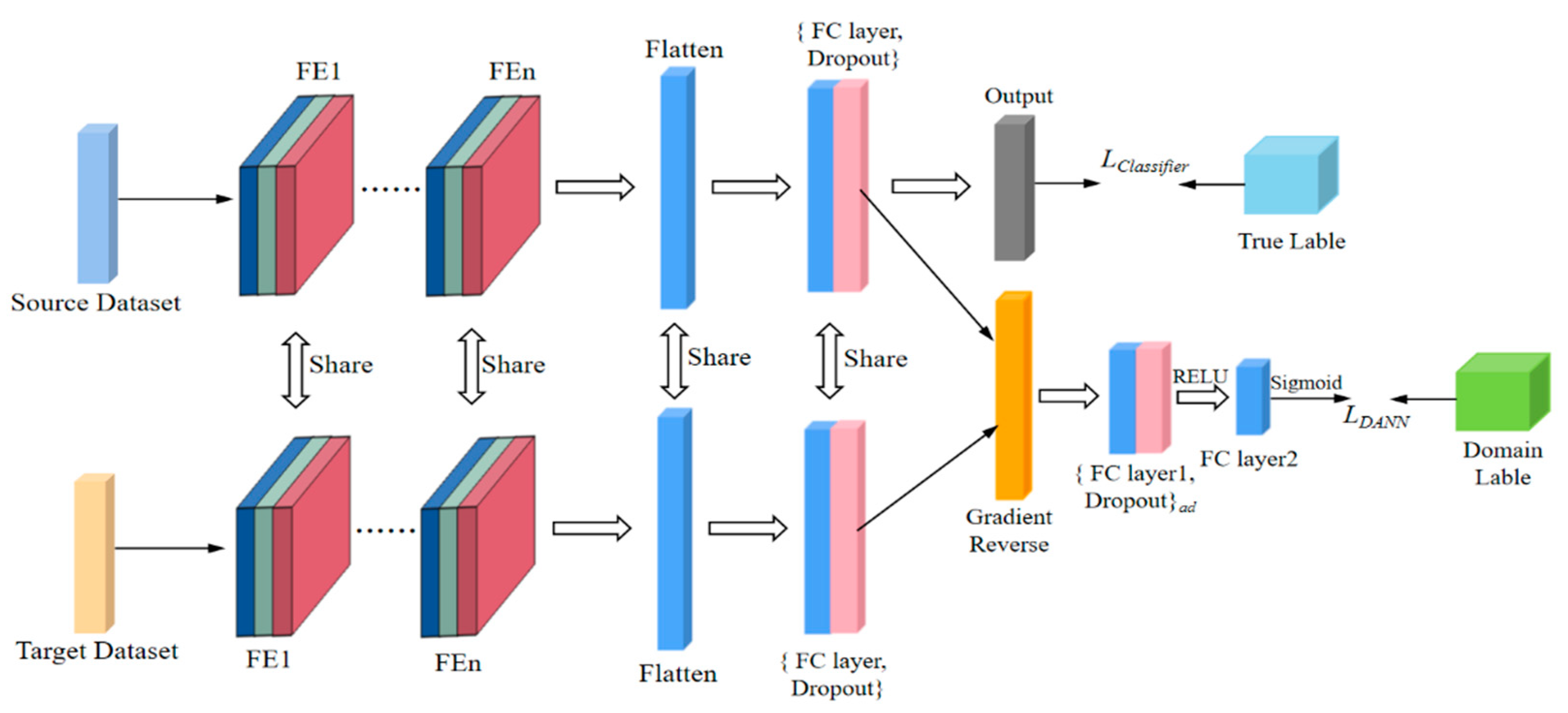
The schematic diagram of JMMD’s training model is shown in Figure 1. On the far left is the dataset, with the top representing the source dataset and the bottom representing the target dataset. These datasets are processed through n layers of feature extractors. Both the source and target datasets pass through the same feature extraction module, typically composed of CNNs or other deep neural networks. These feature extraction layers are shared, allowing both the source and target domains to utilize the same feature extraction network. After feature extraction, the outputs are flattened and processed through fully connected layers (FC layers) and Dropout to ensure that the subsequent comparison and alignment are conducted in the same dimensional space. Additionally, $E_s$ and $E_t$ represent the expected values calculated from the source domain data, where s and t denote specific features or labels of the source or target domains. L represents the loss function.

JMMD considers both differences in input and output feature distributions. As shown in the figure, the input features integrated from the source and target domains in JMMD first undergo tensor product operations with their respective domain outputs. The results are then further processed, including expectation calculation and Hilbert norm operations, to ultimately obtain the JMMD loss value $L_{JMMD}$. The total loss function of the model is presented in Equation (2).

$$L=L_{Classifier}+{\lambda }_{JMMD}{L}_{JMMD}(D_S,D_T)$$

(2)

where $\lambda$ is the weighting coefficient.

JMMD employs the concept of joint distribution and introduces an inter-domain correlation loss, integrating the differences between input and output features. This approach captures both domain differences and commonalities, thereby enhancing the adaptability of the diagnostic model.

2.2. Adversarial-Based Domain Adaptation Methods

To better align the features between the source domain and the target domain and reduce the gap between domains, domain adaptation methods based on inter-domain feature adversarial techniques have been developed from feature mapping domain adaptation methods. The core idea of adversarial-based domain adaptation methods is inspired by the discriminator in Generative Adversarial Networks (GANs). The aim is to repeatedly train the feature extraction layer with the adversarial loss $L_{Adversarial}$ as the objective until its output features are indistinguishable by the domain classification discriminator. This ultimately achieves feature alignment between domains and enhances domain adaptation capability.

Similar to the feature mapping methods, domain adversarial methods can also be divided into two types: those that only consider the difference in input feature distribution, i.e., $P(X_s)\ne Q(X_T)$, and those that consider both the difference in input feature distribution and the difference in joint input-output feature distribution, i.e., $P(X_s,Y_s)\ne Q(X_t,Y_s)$. The former is defined as a Domain Adversarial Neural Network (DANN), or simply DAN; while the latter is called a Conditional Domain Adversarial Network (CDAN), or simply JAN. The schematic diagram of the DAN training model is shown in Figure 2.

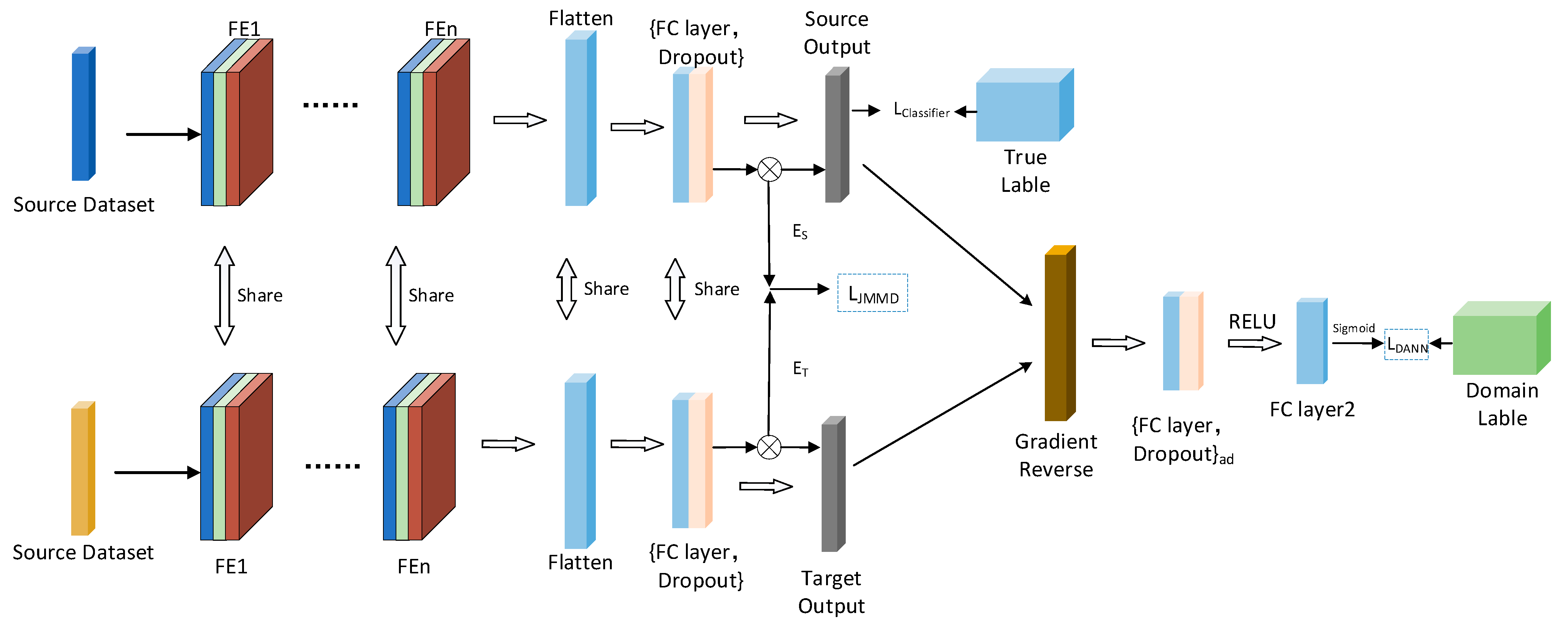
In Figure 2, it can be seen that the DAN domain adaptation method is quite similar to JMMD, as both extract features from the source and target domains through feature extraction layers. These features are then fed into a domain discriminator composed of two fully connected layers. However, a key difference is that DAN includes a gradient reversal process, which is the core component of the DAN method. During the forward pass, the gradient reversal layer functions like a standard layer, passing the features from both the source and target domains. However, during backpropagation, it reverses the sign of the gradients, encouraging the feature extraction network to produce adversarial effects during updates. Through this mechanism, the network is forced to learn domain-invariant features, thus reducing the discrepancy between the domains. After the gradient reversal layer, the features are passed to a domain classifier module. The domain classifier consists of two fully connected layers (denoted as FC layer1 and FC layer2 in the figure), where FC layer1 uses the ReLU activation function, and FC layer2 applies the Sigmoid function. During training, L_DAN progressively increases to hinder the discriminator’s ability to distinguish between domains, thereby minimizing the domain gap. The calculation of L_DAN is given in Equation (3).

$$L_{DAN}({\theta }_f,{\theta }_d)=-E_{x_i^S\in D_S}\log [G_d(G_f(x_i^s;{\theta }_f);{\theta }_d)]-E_{x_j^T\in {\mathcal{D}}_t}\log [1-G_d(G_f(x_j^T;{\theta }_f);{\theta }_d)]$$

(3)

Let ${\theta }_f$ represent the parameters of the feature extraction network, which extracts the feature representations of samples from both the source and target domains, while ${\theta }_d$ represents the parameters of the domain classifier, which determines whether the features of a sample come from the source or target domain. Let $G_f$ represent the feature extraction network and $G_f(x_i^s;{\theta }_f)$ and $G_f(x_j^T;{\theta }_f)$ represent the feature representations of the source and target domain samples $x$ extracted by the feature extraction network, respectively. Let $G_d$ represent the domain classifier, and $G_d(\cdot )$ represent the probability, given by the domain classifier, that a sample $x$ from the source or target domain belongs to the source domain.

It should be noted that the optimization objective of the model training at this time is to reduce the classification loss, $L_{Classifier}$, while increasing the domain adversarial loss, $L_{DAN}$. The expression is in the form of the Equation (4).

$$\begin{array}{l}(\begin{array}{c}{\widehat{\theta }}_f,{\widehat{\theta }}_c\end{array})=\underset{({\theta }_f,{\theta }_c)}{\arg \min }ℒ({\theta }_f,{\theta }_c,{\widehat{\theta }}_d)\\ \begin{array}{c}{\widehat{\theta }}_d\end{array}=\underset{{\theta }_d}{\arg \max }ℒ({\widehat{\theta }}_f,{\widehat{\theta }}_c,{\theta }_d).\end{array}$$

(4)

where ${\theta }_c$ represents the parameter set of the category classifier.

It can be seen that compared to the total loss function of feature mapping domain adaptation, the two losses in the adversarial domain adaptation method are no longer additive but subtractive. The total loss function of DAN is shown in Equation (5).

$$L({\theta }_c,{\theta }_d,{\theta }_f)=L_c({\theta }_f,{\theta }_c)-{\lambda }_{DANN}{L}_{DANN}({\theta }_f,{\theta }_d)$$

(5)

Furthermore, if the standard normal gradient update method is used to complete the backpropagation training process, L_DANN will decrease together with $L_{Classifier}$. Therefore, as can be seen from the above figure, a gradient reversal layer is introduced into Gd and G_f to address this issue. The gradient update method after introducing the gradient reversal layer is as shown in Equations (6)–(8).

$${\theta }_c\leftarrow {\theta }_c-\mu {\displaystyle \frac{\partial L_c^i}{\partial L_c}}$$

(6)

$${\theta }_f\leftarrow {\theta }_f-\mu \left({\displaystyle \frac{\partial L_y^i}{\partial {\theta }_f}}-\lambda {\displaystyle \frac{\partial L_d^i}{\partial {\theta }_f}}\right)$$

(7)

$${\theta }_d\leftarrow {\theta }_d-\mu \lambda {\displaystyle \frac{\partial L_d^i}{\partial {\theta }_d}}$$

(8)

It can be seen that the introduction of the gradient reversal layer corrected the gradient update method for $G_f$.

3. Fusion Domain Adaptation Methods

By combining the powerful deep feature extraction capabilities of CNN with the idea of knowledge transfer, we propose the Fusion Deep Domain Adaptation fault diagnosis model. Leveraging the commonalities of various domain adaptation methods, we integrate the JMMD and DAN methods to propose the FDA fault diagnosis model, further enhancing the fault diagnosis performance in the varying domain and improving the model’s generalization and environmental adaptability.

3.1. Fusion Domain Adaptation

Different domain adaptation methods have their own advantages and characteristics, showcasing both distinctions and commonalities. In the two domain adaptation methods discussed above, during the feature extraction and classification processes, the source domain and target domain share the same network structure. Unlike conventional CNNs, a Dropout layer is introduced after the fully connected layer in each domain adaptation method, which enhances the performance of the domain adaptation model and its generalization ability and reduces the risk of overfitting. However, it is crucial to note that Dropout randomly deactivates neurons during training. Therefore, during the inference or testing phase, Dropout should be turned off to ensure deterministic prediction results.

Feature mapping methods are generally more intuitive and easier to comprehend. They learn a mapping function to map the feature spaces of the source domain and target domain to a shared feature space. Since these methods do not require additional adversarial network training, they typically exhibit higher computational efficiency and lower computational costs. However, they cannot directly handle the nonlinear differences between the target domain and the source domain and may lead to poor performance when faced with complex distributional differences. Adversarial domain adaptation methods introduce an adversarial loss function. By training a generator to produce samples resembling those of the target domain and simultaneously training a discriminator to distinguish between samples from the source domain and the target domain, these methods force the model to learn shared features between the source and target domains. This helps to better match the underlying distributions, handle complex nonlinear relationships between the source and target domains, generate more realistic target domain samples, and exhibit increased robustness to noise and interference. They can better adapt to changes in the target domain distribution. However, the training process of adversarial domain adaptation methods is more complex, as it requires the simultaneous optimization of both the generator and the discriminator and usually involves higher training time and computational costs.

In feature mapping methods, the JMMD approach typically requires only a single feature extractor and one MMD loss function, eliminating the need to train multiple networks or components. This simplifies the model structure and training process. JMMD primarily relies on feature differences between domains rather than label information, allowing it to perform domain adaptation effectively even without target domain labels. Additionally, it can be integrated with various types of feature extractors to adapt to different types of data and tasks. As it is based on sample means, it is generally more computationally efficient than some methods that require calculating distance matrices between domains. By minimizing differences in the feature space, it encourages the model to learn more generalized feature representations, thereby improving performance on the target domain.

In domain adversarial adaptation methods, the DAN approach provides an end-to-end training framework, which allows for joint optimization, and a domain classifier under a unified loss function. This simplifies both the model design and training process. The architecture is relatively straightforward and can be easily integrated into various deep learning models, including Convolutional Neural Networks, Recurrent Neural Networks (RNNs), and more, to adapt to different types of data and tasks. Through adversarial training of the domain classifier, DAN explicitly forces the feature extractor to generate domain-invariant feature representations, thereby enhancing the model’s domain invariance and generalization capabilities. Using a single domain classifier to adversarially train the feature extractor promotes effective feature alignment between the source and target domains, thus improving domain adaptation performance. The domain adversarial loss and classification loss are balanced through a parameter $\lambda$, allowing the model’s domain adaptation performance to be further optimized by adjusting this parameter.

Feature mapping and adversarial networks each enhance the domain adaptation capability of diagnostic models by introducing the mapping distance metric function $L_{Metric}$ and the adversarial loss $L_{Adversarial}$ into the overall loss function $L$. Incorporating both $L_{Metric}$ and $L_{Adversarial}$ into the total loss L allows for the integration of their respective capabilities in capturing inter-domain feature differences.

JMMD and DAN are both capable of adapting well to various feature extractors and are particularly suitable for use with CNNs to capture data features. To leverage their advantages, JMMD and DAN can be fused into a new Fusion Domain Adaptation method, referred to as FDA. The JMMD loss function and the DAN loss function can be simultaneously incorporated into the total loss $L$. The formula for calculating the total loss function in a unified form is shown in Formula (9).

$$L=L_{Classifier}+{\lambda }_{Metric}{L}_{Metric}(D_S,D_T)+{\lambda }_{Adversarial}{L}_{Adversarial}(D_S,D_T)$$

(9)

$L_{Metric}$ and $L_{Adversarial}$ represent the mapping distance metric function and adversarial loss function, respectively. ${\lambda }_{Metric}$ and ${\lambda }_{Adversarial}$ represent their weight coefficients, respectively. $D_S$ and $D_T$ respectively the source domain and the target domain.

The FDA training model diagram after integrating the two methods is shown in Figure 3. Both adversarial domain adaptation methods and feature mapping effectively enhance the domain adaptation capability of diagnostic models by introducing the mapping distance metric function $L_{Metric}$ and the adversarial loss $L_{Adversarial}$ into the total loss function L. The FDA algorithm effectively combines the strengths of both approaches by adjusting the parameter weights. Feature mapping methods have limited capacity to learn local structural information of features, while adversarial methods can better preserve local feature information through the “deception” of the discriminator. The combination of the two can enhance the capture of inter-domain feature differences and improve diagnostic efficiency.

3.2. Fusion Domain Adaptation Diagnostic Process

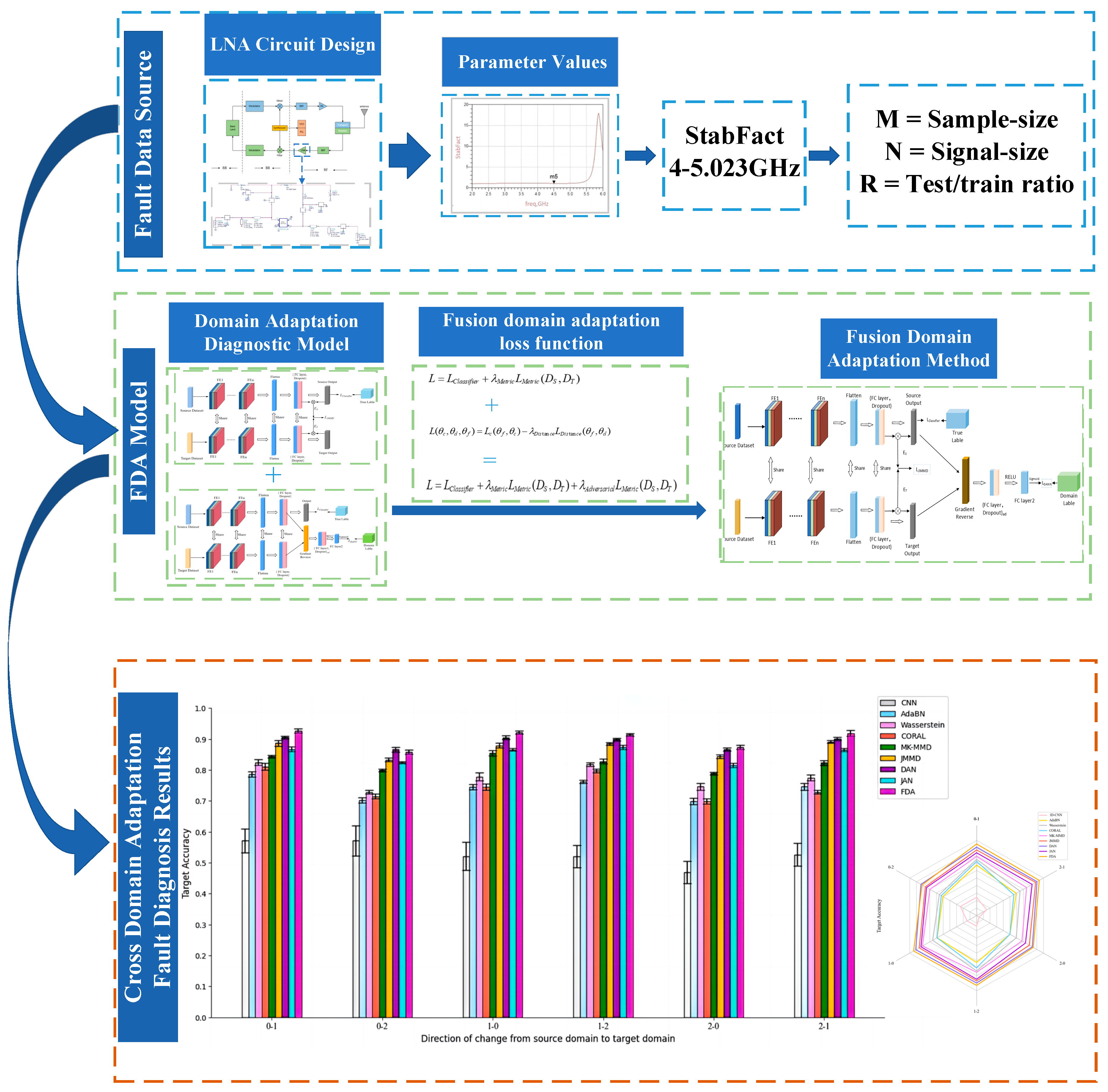
The next step involves conducting cross-domain experiments using an LNA with an operating frequency of 4.5 GHz to validate the feasibility of the proposed method. By integrating the robust deep feature extraction capabilities of CNNs with the concept of knowledge transfer, we propose a fusion deep domain adaptation model for LNA fault diagnosis. This model fuses domain adaptation techniques with CNNs to optimize performance under varying internal and external conditions. Based on the proposed FDA diagnostic model, fault diagnosis will be carried out to evaluate the performance improvements achieved through the fusion domain adaptation approach. Figure 4 illustrates the workflow of the fault diagnosis process utilizing the fusion domain adaptation method.

Based on the figure, the experimental procedure is as follows:

• Design an appropriate low-noise amplifier (LNA) circuit and select a range of fault states. These fault states will be used to simulate various fault conditions encountered in practical applications, ensuring that the proposed method can be effectively validated across diverse scenarios.
• Conduct actual testing of the designed LNA circuit to collect relevant electrical parameter data. This data will be processed and analyzed to construct source and target domain datasets. It is crucial to ensure the quality and representativeness of the datasets to provide accurate information for subsequent model training and evaluation.
• Inject the acquired data into the proposed fusion deep domain adaptation model. Utilize this model for feature extraction, extracting deep features from the data and performing fault diagnosis. By comparing features from the source and target domains, optimize the model’s domain adaptation performance to enhance diagnostic accuracy under varying operational conditions.
• Conduct a detailed analysis of the experimental results to assess the performance improvement achieved by the proposed method. Compare the performance of the fusion domain adaptation approach with traditional methods in terms of accuracy, stability, and robustness. Summarize the findings to provide valuable feedback and recommendations for further research and practical applications.

4. Experimental Validation

4.1. Source of Experimental Data

4.1.1. LNA Circuit

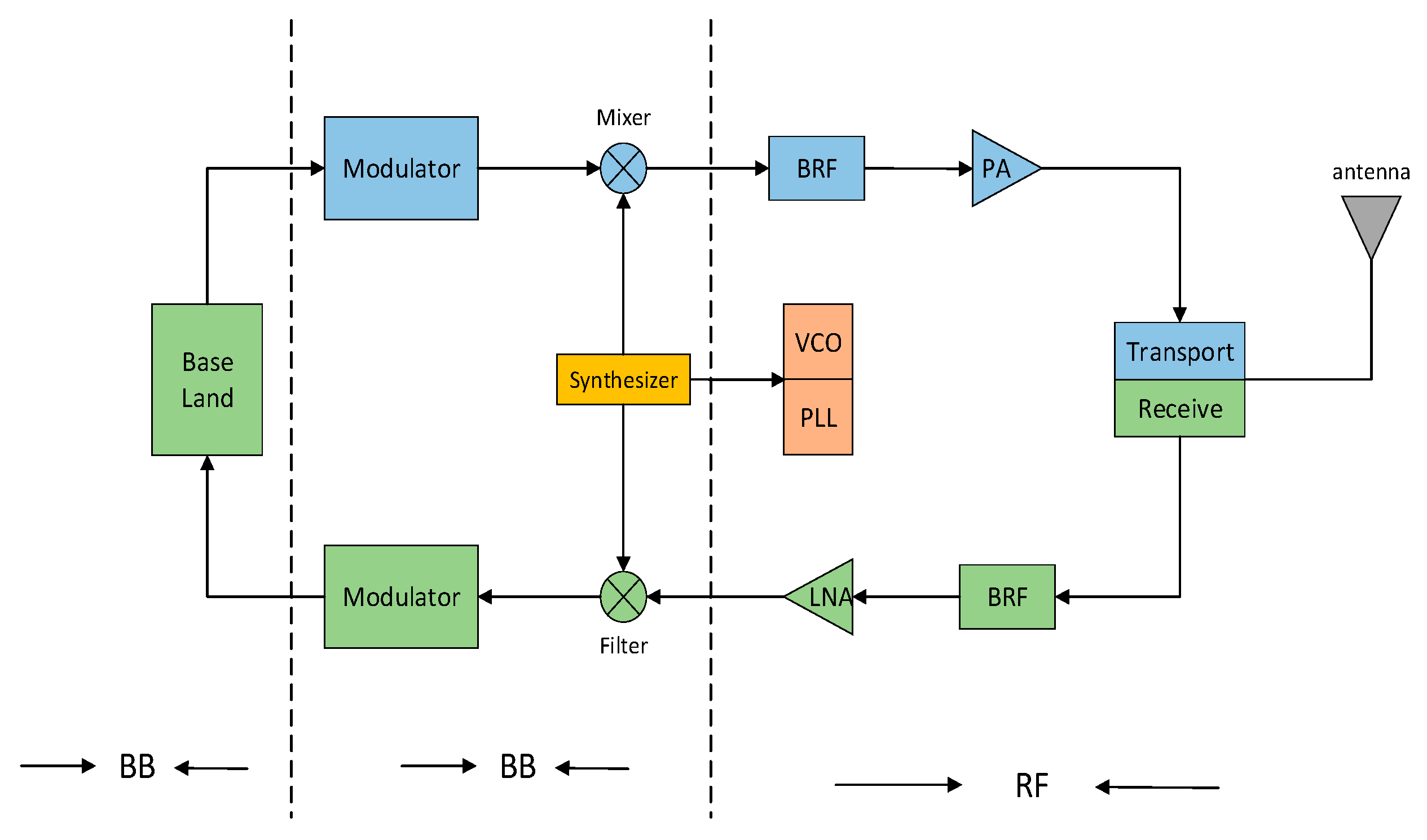
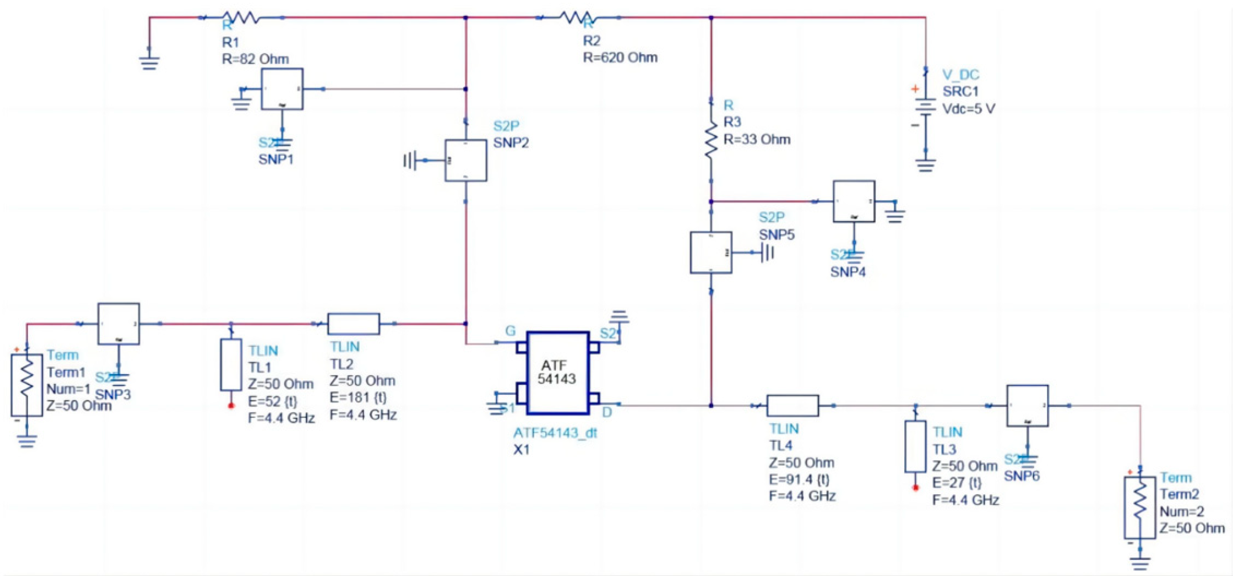
The LNA is a critical component in radio frequency receivers, significantly influencing subsequent encoding, decoding, and signal processing. It compensates for signal attenuation and mitigates interference by providing amplification gain while maintaining a low noise figure, thereby improving the signal-to-noise ratio and overall system performance. The LNA’s gain and noise performance are stable across varying operating conditions, with minimal distortion. This study focuses on the LNA for RF circuit fault diagnosis, offering valuable insights and a foundation for diagnosing faults in other RF system integrated circuits. Figure 5 shows the MIRFS Transceiver Signal Flow Diagram. The transistor chip design utilizes the ATF54143 chip from Avago (San Jose, CA, USA), and the final simulation schematic of the LNA circuit is illustrated in Figure 6.

Hard faults refer to physical damage or failure in circuits, typically caused by component malfunction, damage, or aging. Examples include burnt-out chips, open circuits in resistors, or short circuits in capacitors. Such faults are persistent and require repair or replacement of hardware to resolve. In contrast, soft faults refer to functional anomalies caused by temporary malfunctions or system errors, without any physical damage to the circuit itself. Examples include bit errors, issues that disappear after a system reboot, or errors caused by brief voltage fluctuations. These faults are often induced by environmental factors, operational mistakes, or software issues and can typically be resolved by rebooting or correcting the operation. Furthermore, faults can be categorized based on the number of component failures. Statistical data indicates that single faults constitute approximately 80% of total faults, representing a major proportion of fault occurrences. The LNA in this study comprises nine circuit components, including R1–R3 and SNP1–SNP6. This research primarily focuses on hard faults. Each component exhibits two types of hard fault modes, short circuit and open circuit, along with the healthy state. This results in a total of 19 fault states, labeled from H0 to H18.

4.1.2. Selection of Feature Fault Parameters

Due to circuit aging over time and environmental influences, components may gradually deteriorate or fail entirely. As a result, the performance parameters that reflect the specific operating state of the LNA may deviate from their nominal values. Thus, obtaining these performance parameters can provide a basis for diagnosing circuit faults and identifying the fault type.

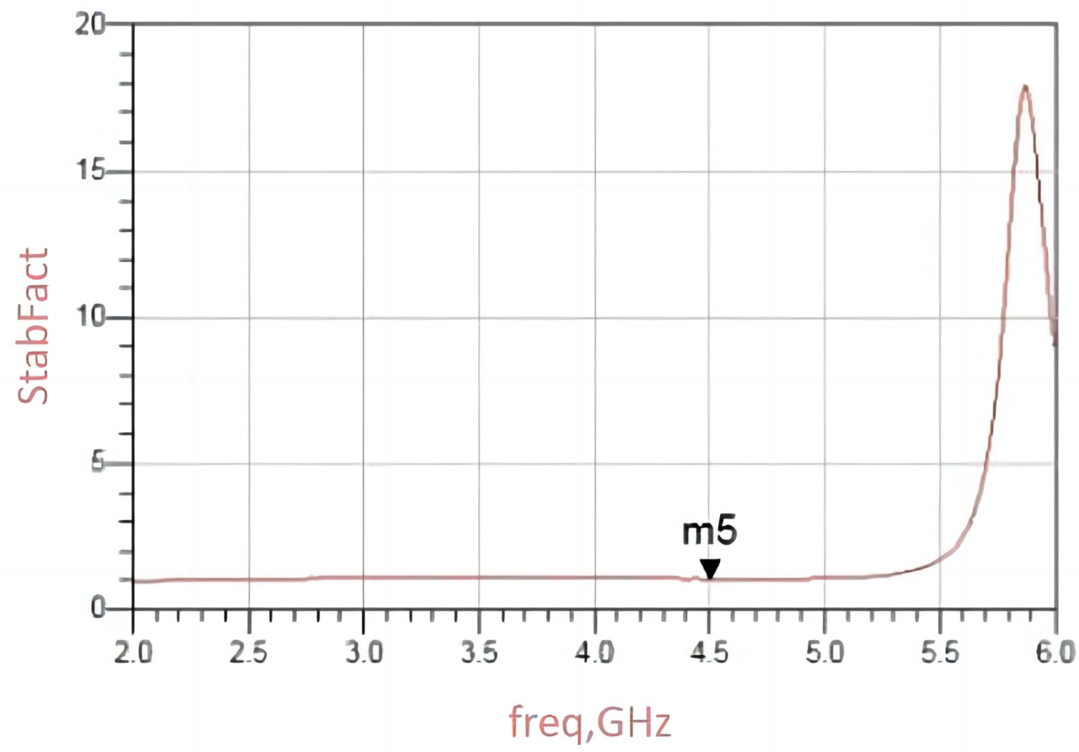
During the actual operation of an LNA, various parameters are used to evaluate its performance, such as S-parameters, stability factor (StabFact), Gain, and noise figure (NF). Among these performance parameters, the StabFact is the key parameter of focus in this study, with the normal operating frequency of the LNA under study being 4.5 GHz. Figure 7 shows the simulated StabFact values within a frequency scanning range of 2 to 6 GHz.

Table 1. StabFact Parameters under Different Health Conditions.

Fault Type	StabFact	Fault Type	StabFact
Health (H0)	1.029	SNP2 open circuit (H10)	1.316
R1 short circuit (H1)	1.325	SNP3 short circuit (H11)	2.179
R1 open circuit (H2)	1.057	SNP3 open circuit (H12)	Invalid
R2 short circuit (H3)	1.057	SNP4 short circuit (H13)	1.223
R2 open circuit (H4)	1.327	SNP4 open circuit (H14)	1.030
R3 short circuit (H5)	1.023	SNP5 short circuit (H15)	2.635
R3 open circuit (H6)	1.224	SNP5 open circuit (H16)	1.224
SNP1 short circuit (H7)	1.325	SNP6 short circuit (H17)	1.032
SNP1 open circuit (H8)	1.065	SNP6 open circuit (H18)	Invalid
SNP2 short circuit (H9)	1.682	-	-

presents the StabFact parameters corresponding to various health states at an operating frequency of 4.5 GHz. Invalid data is observed for states H12 and H18, which can be attributed to open circuits at the input and output ports.

Table 2. StabFact Parameters at different temperature states.

Temperature (°C)	StabFact	Temperature (°C)	StabFact
0	1.028	60	1.029
10	1.028	70	1.029
20	1.029	80	1.029
30	1.029	90	1.029
40	1.029	100	1.029
50	1.029	110	1.028

illustrates the StabFact parameters across different temperature conditions when the system operates in the H0 state at a frequency of 4.5 GHz.

From the two tables above, it is evident that when diagnosing faults under a single operating frequency of 4.5 GHz, there is a problem with the hard fault performance parameters being too similar between different hard faults and under different temperatures, which makes it challenging to classify faults. Additionally, having more fault performance parameters is not necessarily beneficial. Different faults may exhibit identical values for certain performance parameters. If these identical parameters are used to distinguish faults, this will result in feature redundancy and increase the complexity of fault classification. Therefore, a frequency scanning range of 4 to 5.023 GHz was selected with a step size of 1 MHz and a sequence length of 1024. Datasets from the LNA circuit under three different temperature conditions (0 °C, 25 °C, and 50 °C) were chosen as distinct diagnostic datasets, denoted as 0, 1, and 2, respectively.

4.2. LNA Fault Domain Adaptation Diagnostic Experiment

4.2.1. Method Parameter Settings

In this section, we will conduct cross-domain diagnostic experiments on LNAs using various datasets. Figure 8 illustrates the shared backbone network structure of the domain adaptation model. The source and target datasets are vectors of size 1024 × 1, indicating that each sample has a feature dimension of 1024. The model sequentially passes through three sets of convolutional layers, max-pooling layers, and batch normalization layers, which are employed to progressively extract high-level features. ReLU activation is applied to the convolutional layers, transforming the input dimensions from 1024 × 1 to 128 × 16. The output of the convolutional layers is then flattened into a one-dimensional vector of size 1024 × 1, which is subsequently fed into the fully connected layer. This fully connected layer consists of 128 nodes and incorporates Dropout to mitigate overfitting. The final output corresponds to the fault type, representing the model’s ultimate diagnostic result. This shared backbone structure ensures that the source and target domains are unified in the feature space, thereby enhancing the accuracy of domain adaptation tasks.

This study utilizes datasets where each dataset contains 200 samples, with each sample having a signal dimension of 1024. In the experiments, the data will be divided into a test set and a training set, with the test set comprising 20% of the data and the remaining 80% used for training. The model will be trained for 150 epochs to fully leverage the data and ensure convergence during the training process.

Specific data are provided in

Table 3. Sample Data Parameters.

Sample size	200
Signal size	1024
Test/train ratio	20%
Training epochs	150

.

Table 4. Method Parameter Settings.

	Dropout-Rate = 64
Instance-based	AdaBN	batch size
Feature-mapping-based	MK-MMD	kernel size = 5
	JMMD	kernel size = 5
Adversarial-based	DAN	Discriminator fully connected layer = 1	Number of neurons = 256
	JAN	Discriminator fully connected layer = 2	Number of neurons = 128

lists certain special parameters that need to be set individually for various methods during the training process.

4.2.2. Experimental Results Comparison

The CNN diagnostic model is trained under specific environmental and internal conditions. However, in practical applications, variations in these conditions can cause data shifts, leading to a sharp decrease in fault diagnosis accuracy. The issue arises because changes in environmental and internal conditions can cause data distribution shifts, resulting in differences in data feature information and leading to domain shift problems where the data distribution before and after changes are inconsistent. Domain adaptation methods can extract domain-invariant features from data with distribution differences under varying conditions. This enhances the ability to distinguish data from different domains, reduces the negative impact caused by domain shifts, and improves the robustness of the diagnostic model.

Table 5. Diagnostic Accuracy.

Method	Direction of Change from Source Domain to Target Domain
	0→1	0→2	1→0	1→2	2→0	2→1	Avg
CNN	57.14%	57.13%	52.13%	52.08%	46.90%	52.6%	53.00%
AdaBN	78.59%	70.24%	74.48%	76.22%	69.95%	74.61%	74.02%
Wasserstein	82.45%	72.87%	77.84%	81.84%	74.61%	77.45%	77.84%
CORAL	81.05%	71.45%	74.55%	79.74%	69.90%	72.84%	74.92%
MK-MMD	84.37%	79.92%	85.47%	82.76%	78.92%	82.34%	82.30%
JMMD	88.66%	83.32%	87.95%	88.50%	84.39%	89.13%	86.99%
DAN	90.55%	86.60%	90.50%	89.87%	86.63%	90.16%	89.05%
JAN	86.76%	82.40%	86.58%	87.37%	81.55%	86.50%	85.19%
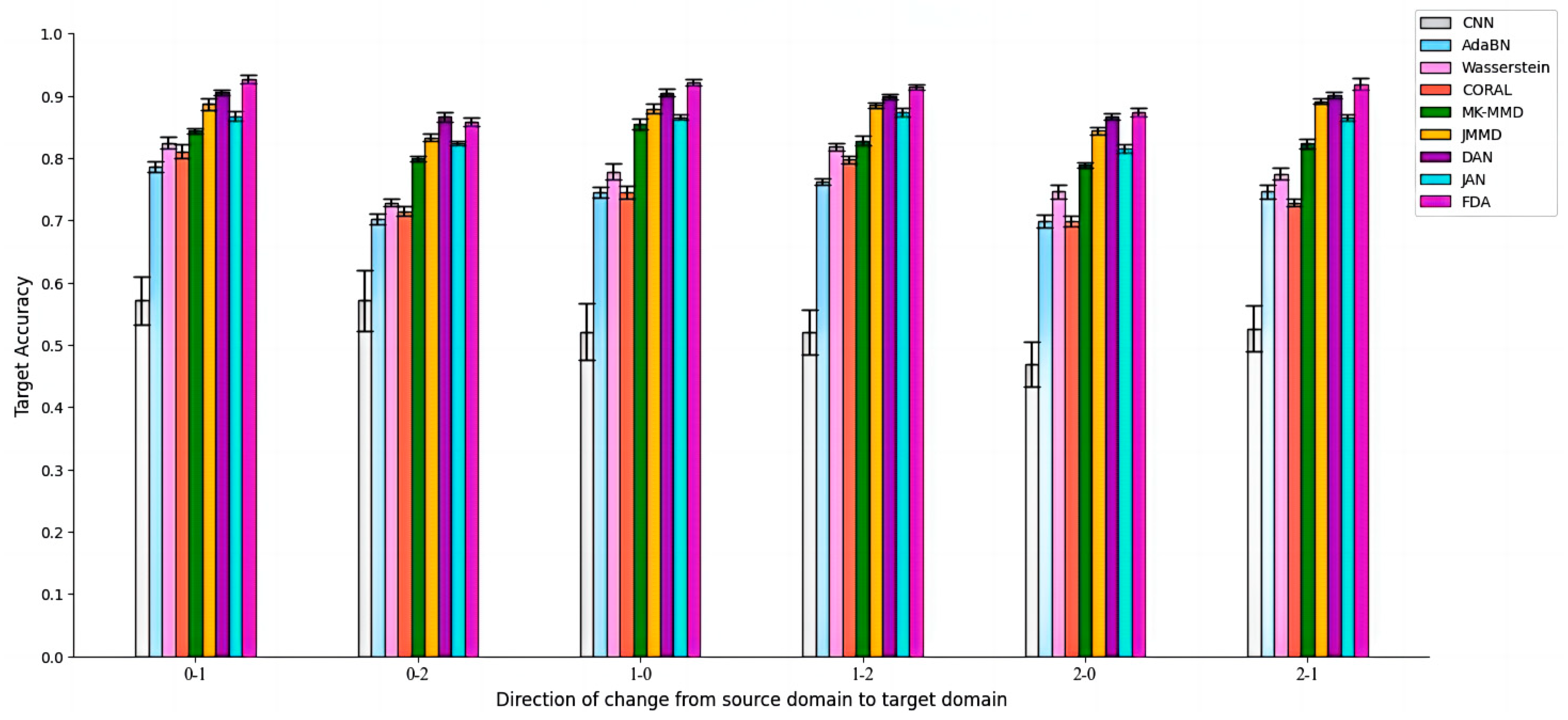
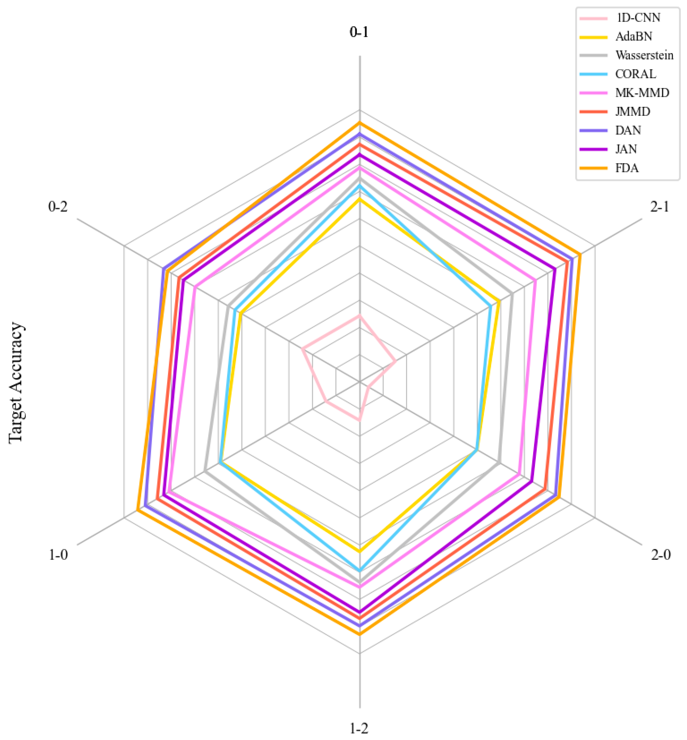
FDA	92.63%	85.78%	92.10%	91.44%	87.36%	91.84%	90.19%

shows the fault diagnosis accuracy of different methods during the training process across various source and target domains. Figure 9 and Figure 10 illustrate the results of CNN and various domain adaptation methods in cross-domain fault diagnosis.

It can be observed that while the CNN method performs well under constant external conditions, its accuracy significantly drops to below 60%—with a minimum of 47%—when there is a mismatch between the source and target domain datasets. This decline, accompanied by substantial diagnostic errors, indicates that the CNN model exhibits poor adaptability to domain changes. The AdaBN method, with a batch size of 64, enhances adaptability to domain changes by aligning with the data distribution of the target domain. Compared to the CNN method without domain adaptation (which has a diagnostic accuracy of approximately 50%), AdaBN increases the average accuracy in the target domain by about 20%. Furthermore, the reduction in error in the target domain suggests improved diagnostic stability at the target domain. Among the various feature mapping methods, all but CORAL show improved cross-domain diagnostic accuracy. JMMD, as the mapping function, achieves the highest accuracy, reaching up to 89.13% across different transitions. In domain adversarial methods, DAN, which considers only the input feature distribution, achieves a higher accuracy of up to 90.55% compared to JAN, which is trained with joint distribution adversarial training. Finally, the proposed FDA method demonstrates the highest average diagnostic accuracy, reaching 90.19%. This method outperforms general domain adaptation methods, except for the 0–2 scenario, underscoring its effectiveness in enhancing cross-domain diagnostic accuracy.

Figure 10 intuitively illustrates the superiority of the FDA fusion domain adaptation method in cross-domain fault diagnosis. Its diagnostic performance from the source domain to the target domain is excellent, with overall high-quality performance, making it suitable for diagnosing various types of faults In different environments and conditions.

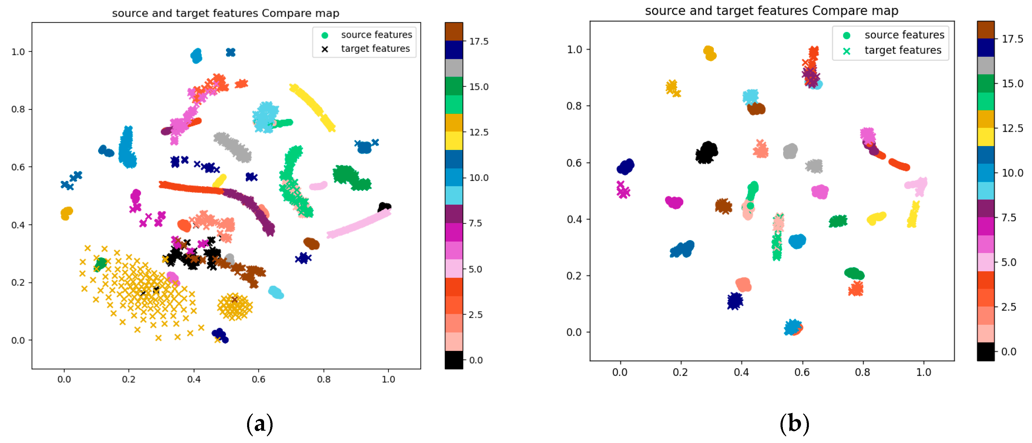
To further intuitively illustrate the improvement in alignment between various fault feature domains at the initial and target domains using different domain adaptation methods, t-SNE dimensionality reduction was applied to the diagnostic output features of the CNN and FDA domain adaptation methods during the 1–0 domain transition. The reduced-dimensional feature map is shown in Figure 11.

From the reduced-dimensional feature map, it can be observed that the domain adaptation methods do not significantly impact the clustering of features in the source and target domains. However, in the CNN method, there is noticeable dispersion in the fault features, and a considerable overlap between the source and target domain feature clusters, indicating poor cross-domain fault diagnosis performance. The proposed method outperforms the CNN algorithm in extracting clustering features for fault types in the target domain. Although some overlap of different fault features still exists, the alignment effect is clearly better than that of CNN.

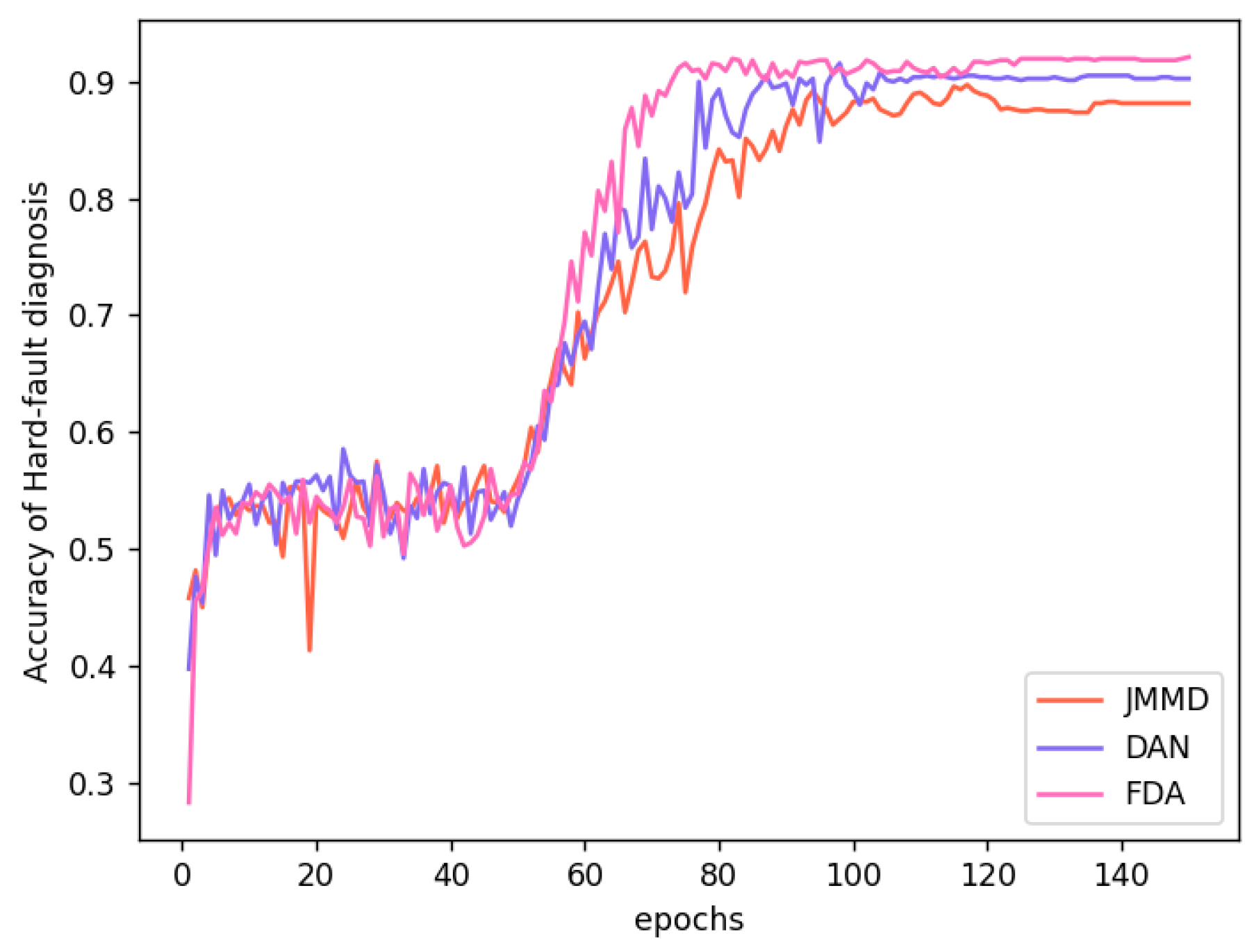
Figure 12 presents the accuracy diagrams of the target domain training processes for JMMD, DAN, and FDA. The graph clearly shows that after combining the two domain adaptation methods, the diagnostic accuracy improved by nearly 2%. The convergence speed of the model has also been enhanced, suggesting an improvement in capturing domain feature difference information efficiently.

4.3. Impact of Method Parameters

While the above content compared domain adaptation methods with CNN and fusion domain adaptation methods with general domain adaptation methods, variations in parameter settings, as well as differences in training and test set allocations for each method may still affect the diagnostic efficiency, accuracy, and the fairness of the comparisons. The following section discusses the impact of parameter settings on the fault diagnosis accuracy for each method.

4.3.1. Dropout-Rate Parameters

A Dropout layer was added after the fully connected layer in various domain adaptation methods to enhance the model’s performance when generalizing to the target domain. The most critical hyperparameter in the Dropout layer is the Dropout rate. A rate that is too high results in discarding too many neurons, leading to unstable model classification and underfitting. Conversely, a rate that is too low may cause the model to overly rely on the source domain training data. Furthermore, the premise of enhancing generalization by adding Dropout is that the diagnostic accuracy of the model trained on the source domain dataset remains unaffected.

To investigate the impact of the Dropout rate on diagnostic performance, experiments were conducted using the 25 °C LNA hard fault diagnosis as an example. The experimental results are presented in

Table 6. Comparison Table of the Impact of Dropout Rate on Diagnostic Performance.

Dropout Rate	0.1	0.2	0.3	0.4	0.5	0.6	0.7	0.8	0.9
Training set (%)	97.75	97.47	97.16	97.19	95.68	95.44	95.37	91.12	67.93
Testing set (%)	97.26	97.05	97.26	97.58	96.74	96.21	96.32	95.79	85.79

.

From the experimental results, as the Dropout rate increases, the test set accuracy gradually becomes slightly higher than that of the training set, indicating an improvement in the model’s generalization ability. Up to a Dropout rate of 0.5, although the test set continues to exhibit good generalization performance, the accuracies of both the training and test sets begin to decline. This suggests that the proportion of discarded neurons has started to negatively impact the model’s diagnostic performance, and this effect intensifies as the Dropout rate increases further. Therefore, to maintain the model’s performance in the source domain, the Dropout rate is set to 0.4.

4.3.2. Training–Testing Set Ratio

During domain adaptation training, the ratio of the training set to the test set can significantly affect the results. A larger training set provides the model with more data to learn feature relationships, potentially leading to a better fit on the training data. Selecting an appropriate training-to-test-set ratio can enhance the model’s accuracy. Using the FDA method as an example, this study examines the optimal training-to-test-set ratio.

Table 7. Comparison Table of the Impact of Training Set Ratios on Diagnostic Performance.

Train–Test Ratio (%)	Direction of Change from Source Domain to Target Domain
	0→1	0→2	1→0	1→2	2→0	2→1	Avg
20	92.63%	85.78%	92.10%	91.44%	87.36%	91.84%	90.19%
30	90.66%	85.32%	91.95%	90.50%	87.29%	91.13%	89.48%
40	89.55%	84.60%	91.50%	90.87%	86.63%	90.16%	88.89%
50	89.13%	84.65%	91.16%	90.24%	86.36%	90.34%	88.65%

presents the fault diagnosis accuracy of the FDA method under various training set ratios across different cross-domain conditions.

The training set is used to fit the model, while the test set evaluates the model’s performance on unseen data. During domain adaptation training, the ratio of the training set to the test set can significantly affect the results. A larger training set provides the model with more data to learn the relationships between features, potentially improving its ability to fit the training data. Selecting an appropriate training-to-test-set ratio can enhance the model’s accuracy. Using the FDA method as an example, this study investigates the optimal training-to-test-set ratio. Table 7 presents the fault diagnosis accuracy of the FDA method under various training set ratios across different cross-domain conditions.

Analysis of the table shows that the proportion of training and testing sets does not significantly affect the training accuracy in the target domain. However, the overall trend indicates that as the proportion of the testing set increases, diagnostic accuracy decreases. Nonetheless, it is evident that when the testing set comprises 20% of the entire dataset, higher diagnostic accuracy is observed. Therefore, this study uses a 20% testing set as the experimental reference.

4.3.3. Parameters of Each Method

(1)

AdaBN Influence of Training Parameters

AdaBN offers two updating methods for the BN (Batch Normalization) layer: batch updating and full dataset updating. To determine the optimal updating method for the BN layer, we will use the dataset from the 25 °C state as the source domain and the dataset from the 0 °C state as the target domain for fault diagnosis. When using the batch updating method for the BN layer, the batch size directly influences AdaBN’s domain adaptation capability. Therefore, experiments are conducted to examine the impact of batch size on domain adaptation performance, aiming to identify the optimal batch size for BN layer updating. The experimental results are presented in

Table 8. Performance Impact of Batch-Size Variations on BN Layer Batch Updating.

Update Batch Size	8	16	32	64	128	256	512
Source Domain Test Set (%)	96.23	96.41	97.63	97.37	95.92	89.41	84.34
Target Domain Test Set (%)	70.58	71.53	71.68	74.47	73.29	72.50	70.92
Training Duration (s)	505	352	275	235	216	209	206

.

From the comparison experiments on BN layer update batch sizes, it is observed that as the batch size increases beyond 64, the accuracy of the source domain test set begins to gradually decrease. This finding is consistent with the results from CNN batch-size experiments. An excessively large batch size reduces the frequency of updates to the BN layer’s statistical parameters in the target domain, leading to a corresponding decrease in target domain test accuracy. Conversely, an excessively small batch size can make the BN layer’s statistical parameters more susceptible to outlier data, resulting in reduced accuracy in the target domain. Based on the experimental results, a batch size of 64 is identified as optimal for BN layer updates when using batch updating.

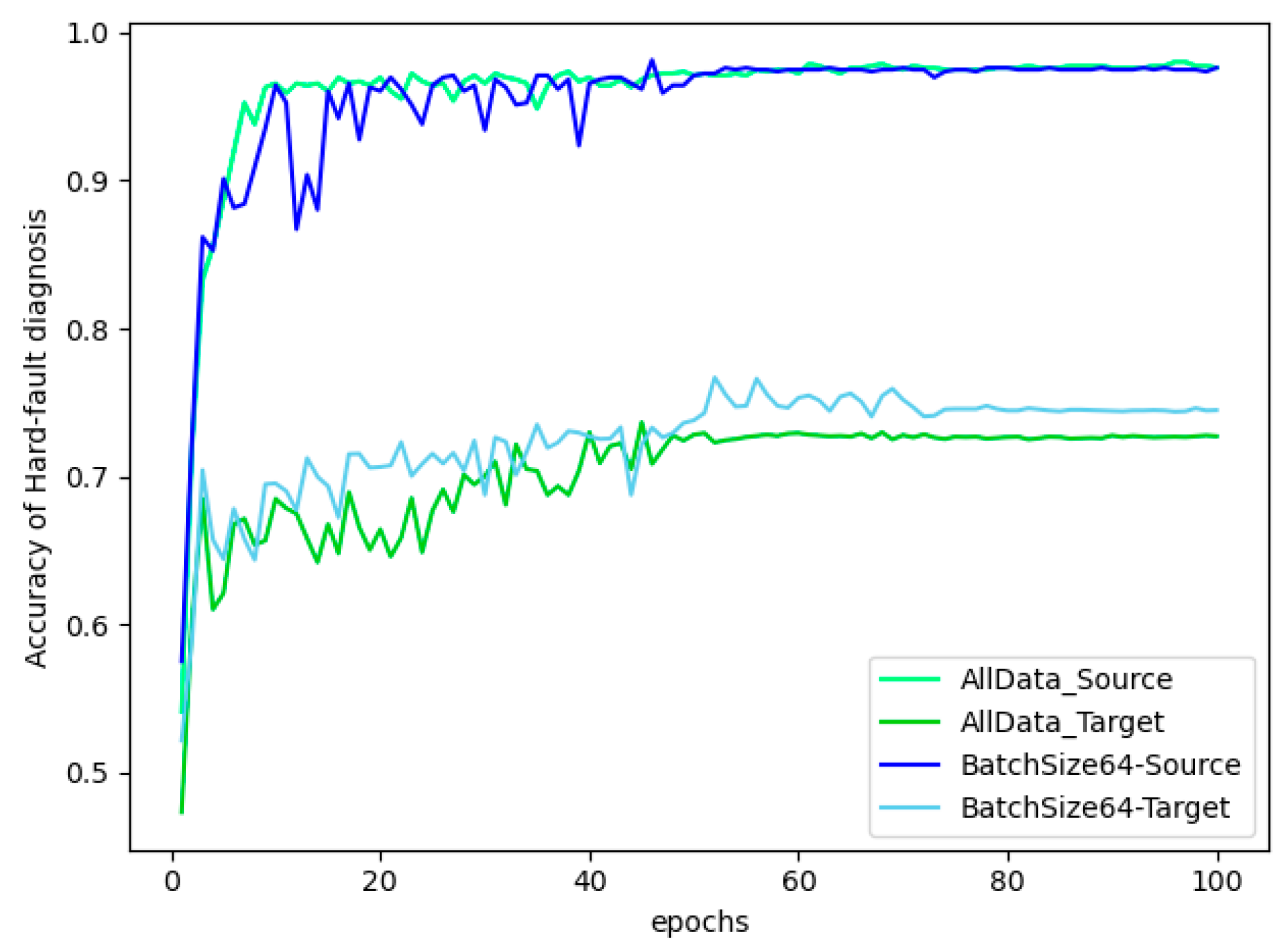
When the BN layer updates using the complete target domain dataset, its domain adaptation performance is not influenced by other hyperparameters. However, the effectiveness of this method compared to the batch update approach still needs to be validated through comparative experiments. Therefore, experiments were conducted using a batch size of 64 for comparison, and the results are shown in Figure 13.

From the comparative experimental results, it can be observed that whether using batch updates or updating the entire target domain dataset, there is no significant impact on the final diagnostic results of the source domain test set. However, the diagnostic results in the target domain, which reflect the model’s domain adaptation characteristics, do differ. With a batch size of 64, the stable accuracy in the target domain is 74.47%, while the stable accuracy with full data updates is 72.71%. Therefore, updating the BN layer using batch mode demonstrates stronger adaptation capabilities in the target domain compared to full data updates.

(2)

Feature Mapping Training Parameters

The domain adaptation capability of the feature mapping method is directly related to the mapping distance metric function, which in turn depends on the accuracy of domain distance calculation and the parameters involved in this process. Specifically, MK-MMD and JMMD are significantly influenced by the type of mapping kernel function (kernel type) and the number of kernels (kernel size).

The choice of kernel function type directly affects the model’s nonlinear mapping capability and domain adaptation generalization performance. Currently, five kernel functions are commonly used: linear, polynomial, sigmoid, Laplacian, and Gaussian Radial Basis Function (RBF). Each has its own characteristics. The Gaussian RBF kernel function is the most widely used and versatile in practical applications, making it the most effective choice for the kernel function in both MK-MMD and JMMD mapping methods.

The choice of kernel size directly impacts the density and dimensionality of the feature space. Additionally, the kernel size affects the bandwidth parameter γ of the RBF, which in turn influences the smoothness and complexity of the model’s decision boundary. Typically, a kernel size that is too large increases both the feature space dimensionality and the bandwidth γ, making the model more complex and raising the risk of overfitting. Conversely, a kernel size that is too small simplifies the feature space and reduces γ, which enhances generalization but sacrifices the model’s ability to capture complex data features. Therefore, determining the appropriate kernel size through gradient change experiments is crucial for measuring distribution differences and improving feature alignment between the source and target domains. Diagnostic tests were conducted using kernel size gradient change experiments and the results are shown in

Table 9. Results of the Kernel Size Gradient Change Experiment.

RBF Kernel Size		1	2	3	4	5	6	7	8	9
MK-MDD	Source (%)	97.36	98.29	97.76	98.16	97.63	98.28	97.50	97.76	97.63
	Target (%)	71.44	75.13	78.82	81.84	86.97	81.45	78.55	75.13	74.08
JMMD	Source (%)	97.89	97.89	98.16	98.03	98.02	97.23	98.29	98.15	97.76
	Target (%)	85.53	86.97	86.97	87.89	88.42	88.95	88.29	81.45	78.85

.

According to the experimental results, the performance of both MK-MMD and JMMD is influenced by changes in kernel size. The performance of MK-MMD is more significantly affected by kernel size, with its performance exhibiting a trend of increasing and then decreasing. For MK-MMD, the highest diagnostic accuracy in the target domain is achieved with a kernel size of 5, whereas for JMMD, the highest diagnostic accuracy is attained with a kernel size of 6. However, the difference in accuracy between kernel sizes 5 and 6 is only 0.53%.

(3)

Domain adversarial discriminator network structure parameters

In adversarial networks, the discriminator primarily consists of fully connected layers. Therefore, the structure of these layers directly impacts the performance of the discriminator in domain adversarial discrimination tasks. The number of layers and the number of neurons in each fully connected layer are hyperparameters that need to be optimized through experiments. For cross-domain diagnostic tasks, the optimized experimental results for the fully connected layer parameters in the discriminators of DAN (Domain Adversarial Network) and JAN (Joint Adversarial Network) are shown in

Table 10. Optimization and Adjustment Experiment of DAN Discriminator Structure Parameters.

Number of FC Layers	Number of Neurons in FC Layers
	16	32	64	128	256	512	1024
1	83.29	84.61	86.05	89.47	90.26	88.16	87.50
2	85.13	86.58	87.24	86.84	86.18	85.39	85.92
3	83.55	85.53	86.97	87.11	85.66	86.32	82.24
4	74.34	75.53	85.53	86.58	83.55	82.89	84.34

and

Table 11. Optimization and Adjustment Experiment of JAN Discriminator Structure Parameters.

Number of FC Layers	Number of Neurons in FC Layers
	16	32	64	128	256	512	1024
1	78.42	81.45	78.82	76.32	73.68	73.95	71.58
2	83.95	84.21	86.05	86.45	84.08	81.84	82.50
3	81.45	82.76	79.87	81.18	79.21	80.13	77.24
4	80.79	80.39	81.45	76.18	73.42	77.76	76.05

.

From the experimental results, it can be observed that for DAN, the discriminator performs well with a single fully connected layer, achieving effective feature alignment between domains during domain adversarial training. The optimal number of neurons for this configuration is 256. In contrast, the JAN discriminator demonstrates the strongest adaptation capability to the target domain with two fully connected layers, each containing 128 neurons. This improved performance may be attributed to the inclusion of joint distributions between output and input, which increases the dimensionality and complexity of the adversarial training features. Consequently, the discriminator benefits from deeper fully connected layers to enhance its nonlinear expression capability and improve domain adaptation. In summary, the optimal structure for DAN is a single layer with 256 neurons, while for JAN, it is two layers with 128 neurons each, which yields the best results for fault diagnosis.

5. Conclusions and Discussion

When environmental factors or internal conditions change in low-noise amplifiers (LNAs), traditional fault diagnosis methods often perform poorly. To address this issue, a fusion fault diagnosis method based on feature mapping and domain adversarial domain adaptation is proposed in this study. The main innovations and contributions are as follows:

(1). Neural-network-based domain adaptation methods are introduced into LNA fault diagnosis for the first time in this study. By modeling and adjusting the distribution differences between the source and target domains, this approach significantly enhances the reliability and efficiency of LNA fault diagnosis.

(2). A diagnostic model that combines CNNs with domain adaptation techniques is proposed. This fusion not only improves the model’s generalization ability and adaptability to environmental changes but also enhances the robustness of the diagnostic technology under different environmental conditions.

(3). An optimized loss function is designed to combine feature domain adaptation with adversarial domain adaptation methods. This function makes full use of information from both the source and target domains. The optimized loss function enhances the model’s domain adaptation capability, thereby improving the overall performance of LNA fault diagnosis.

Experimental results demonstrate the significant effectiveness of the fusion domain adaptation method in hard fault diagnosis. This method achieves a fault diagnosis accuracy of up to 90.19% with minimal diagnostic error. It significantly outperforms traditional CNN methods.

However, the method’s performance for soft fault diagnosis remains suboptimal, especially in cross-domain scenarios where the fault recognition rate does not exceed 50%. Due to the more complex features and higher variability of soft faults, the existing method’s adaptability is limited. Future research will focus on optimizing this method to enhance soft fault diagnosis. This includes exploring more refined feature extraction and domain adversarial strategies. Additionally, integrating advanced machine learning techniques and domain adaptation algorithms will be considered. The goal is to achieve more comprehensive detection and diagnosis of soft faults.

References

1. Das, R.; De, B.P.; Dash, S.K.; Ghosh, S.; Kar, R.; Mandal, D. Optimal Design of 2.4 GHz ISM Band CMOS LNA Using the Cat Swarm Optimization Algorithm. J. Electron. Mater. 2024, 5, 3614–3625. [Google Scholar] [CrossRef]
2. Jing, L.; Lei, C. A broadband low-power LNA design based on 5G applications. Electron. Des. Eng. 2024, 32, 158–162. [Google Scholar]
3. Kun, F. Design of a universal processing module for airborne integrated RF system. Aeronaut. Comput. Tech. 2023, 53, 106–109. [Google Scholar]
4. Lina, S.; Baohua, L.; Yu, C. A test method for compatibility capability of airborne integrated RF system. Sci. Technol. Eng. 2022, 22, 9857–9863. [Google Scholar]
5. Zhang, X.L. Multifunctional Integrated Radio Frequency Technology Development Research. Mod. Radar 2020, 42, 78–81. [Google Scholar]
6. Biye, Q.; Shijun, R. Application and Development of Shipborne Multifunctional Integrated Radio Frequency Systems. Ship Electron. Eng. 2019, 39, 11–14+55. [Google Scholar]
7. Zeng, Z.; Zhang, H.; Miao, Q. Analytical Model Based Fault Diagnosis of Complex System: A Review. In Proceedings of the ICSMD 2021—2nd International Conference on Sensing, Measurement and Data Analytics in the Era of Artificial Intelligence, Nanjing, China, 21–23 October 2021; p. 176353. [Google Scholar]
8. Peng, C.; Li, F.; Jiang, J. Overview of Fault Diagnosis and Prediction Methods Based on Deep Learning. Mod. Electron. Technol. 2022, 45, 111–120. [Google Scholar]
9. Yan, R.; Jian, Y.; Hao, L.C.; Han, X.Y.; Tang, L.L. Research on Automatic Knowledge Acquisition Technology for Software Fault Diagnosis. In Proceedings of the 2019 International Conference on Quality, Reliability, Risk, Maintenance, and Safety Engineering (QR2MSE), Zhangjiajie, China, 6–9 August 2019; pp. 901–907. [Google Scholar]
10. Cheng, L.; Sun, C. A Multi-Level Interactive Intelligent Fault Diagnosis Method for Aviation Electronic Systems. In Proceedings of the 2023 3rd International Conference on Frontiers of Electronics, Information and Computation Technologies (ICFEICT), Yangzhou, China, 26–29 May 2023; pp. 476–481. [Google Scholar]
11. Zhang, H.; Ge, D.; Su, W.; Zhang, L. Fault Diagnosis of Power System Considering Communication System Information Transmission Error. In Proceedings of the 2018 IEEE Power & Energy Society General Meeting (PESGM), Portland, OR, USA, 5–10 August 2018; pp. 1–5. [Google Scholar]
12. Viveros-Wacher, A.; Rayas-Sánchez, J.E. Analog Fault Identification in RF Circuits using Artificial Neural Networks and Constrained Parameter Extraction. In Proceedings of the 2018 IEEE MTT-S International Conference on Numerical Electromagnetic and Multiphysics Modeling and Optimization (NEMO), Reykjavik, Iceland, 8–10 August 2018; pp. 1–3. [Google Scholar]
13. Sun, B.; Wang, J.; He, Z.; Zhou, H.; Gu, F. Fault Identification for a Closed-Loop Control System Based on an Improved Deep Neural Network. Sensors 2019, 19, 2131. [Google Scholar] [CrossRef]
14. Lin, S.C.; Jen, C.W.; Su, S.F.; Huang, Y. A Signal Fusion-based ANN Algorithm for Fault Diagnosis of Rotating Machinery. In Proceedings of the 2020 International Conference on System Science and Engineering (ICSSE), Kagawa, Japan, 31 August–3 September 2020; pp. 1–6. [Google Scholar]
15. He, J.; Li, X.; Chen, Y.; Chen, D.; Guo, J.; Zhou, Y. Deep Transfer Learning Method Based on 1D-CNN for Bearing Fault Diagnosis. Shock Vib. 2021, 2021, 6687331. [Google Scholar] [CrossRef]
16. Gong, B.; Du, X. Research on Analog Circuit Fault Diagnosis Based on CBAM-CNN. In Proceedings of the 2021 IEEE International Conference on Electronic Technology, Communication and Information (ICETCI), Changchun, China, 27–29 August 2021; pp. 258–261. [Google Scholar]
17. Ramírez, I.S.; Márquez, F.P.G.; Chaparro, J.P. Convolutional neural networks and Internet of Things for fault detection by aerial monitoring of photovoltaic solar plants. Measurement 2024, 234, 114861. [Google Scholar] [CrossRef]
18. Zhang, Y.W.; Zang, Z.H.; Zhang, X.M.; Song, L.S.; Yu, Z.L.; Wang, Y.T.; Gao, Y.; Wang, L. Fault Diagnosis of Industrial Robot Based on Multi-Source Data Fusion and Channel Attention Convolutional Neural Networks. IEEE Access 2024, 12, 82247–82260. [Google Scholar] [CrossRef]
19. Yang, X.; Bi, F.; Cheng, J.; Tang, D.; Shen, P.; Bi, X. A Multiple Attention Convolutional Neural Networks for Diesel Engine Fault Diagnosis. Sensors 2024, 24, 2708. [Google Scholar] [CrossRef] [PubMed]
20. Ning, L.; Pei, D.F. Power line fault diagnosis based on convolutional neural networks. Heliyon 2024, 10, e29021. [Google Scholar] [CrossRef] [PubMed]
21. Chung, K.J.; Lin, C.W. Condition monitoring for fault diagnosis of railway wheels using recurrence plots and convolutional neural networks (RP-CNN) models. Meas. Control 2024, 57, 330–338. [Google Scholar] [CrossRef]
22. Kai, W.; Yuanhui, L. Summary of Application of Transfer Learning in Predictive Maintenance of Machinery and Equipment. China Instrum. 2019, 12, 64–68. [Google Scholar]
23. Tastimur, C.; Karakose, M.; Akin, E. Vibration Signal Processing Based Bearing Defect Diagnosis with Transfer Learning. In Proceedings of the 2019 1st International Informatics and Software Engineering Conference (UBMYK), Ankara, Turkey, 6–7 November 2019; pp. 1–5. [Google Scholar]
24. Li, F.; Tang, T.; Tang, B.; He, Q. Deep convolution domain-adversarial transfer learning for fault diagnosis of rolling bearings. Measurement 2021, 169, 108339. [Google Scholar] [CrossRef]
25. Yang, Y.; He, Z.; Yao, H.; Wang, Y.; Feng, J.; Wu, Y. Bearing Fault Diagnosis Method Based on Adversarial Transfer Learning for Imbalanced Samples of Portal Crane Drive Motor. Actuators 2023, 12, 466. [Google Scholar] [CrossRef]
26. Zhang, B.; Dong, H.; Qaid, H.A.A.M.; Wang, Y. Deep Domain Adaptation with Correlation Alignment and Supervised Contrastive Learning for Intelligent Fault Diagnosis in Bearings and Gears of Rotating Machinery. Actuators 2024, 13, 93. [Google Scholar] [CrossRef]
27. Zhang, B.; Li, F.; Ma, N.; Ji, W.; Ng, S.-K. Open Set Bearing Fault Diagnosis with Domain Adaptive Adversarial Network under Varying Conditions. Actuators 2024, 13, 121. [Google Scholar] [CrossRef]
28. Dong, F.; Yang, J.; Cai, Y.; Xie, L. Transfer Learning-Based Fault Diagnosis Method for Marine Turbochargers. Actuators 2023, 12, 146. [Google Scholar] [CrossRef]
29. Zhou, D.Y. Research on Modeling Analysis and Fault Diagnosis Technology for Testing Requirements of Airborne RF System. Master’s Thesis, Northwestern Polytechnical University, Xi’an, China, 2024. [Google Scholar]
30. Xie, S.; Xia, P.; Zhang, H. Domain adaptation with domain specific information and feature disentanglement for bearing fault diagnosis. Meas. Sci. Technol. 2024, 35, 056101. [Google Scholar] [CrossRef]
31. Choi, J.; Kong, D.; Cho, H. Weighted Domain Adaptation Using the Graph-Structured Dataset Representation for Machinery Fault Diagnosis under Varying Operating Conditions. Sensors 2024, 24, 188. [Google Scholar] [CrossRef] [PubMed]
32. Nejjar, I.; Geissmann, F.; Zhao, M.; Taal, C.; Fink, O. Domain adaptation via alignment of operation profile for Remaining Useful Lifetime prediction. Reliab. Eng. Syst. Saf. 2024, 242, 109718. [Google Scholar] [CrossRef]
33. Lee, J.; Ko, J.U.; Kim, T.; Kim, Y.C.; Ha Jung, J.; Youn, B.D. Domain adaptation with label-aligned sampling (DALAS) for cross-domain fault diagnosis of rotating machinery under class imbalance. Expert Syst. Appl. 2024, 243, 122910. [Google Scholar] [CrossRef]
34. Zhang, Y.F.; He, Y.; Tang, H.S.; Ren, Y.; Xiang, J.W. Adversarial Domain Adaptation Approach for Axial Piston Pump Fault Diagnosis Under Small Sample Condition Based on Measured and Simulated Signals. IEEE Trans. Instrum. Meas. 2024, 73, 3518812. [Google Scholar] [CrossRef]
35. Hasan, M.J.; Kim, J.-M. Bearing Fault Diagnosis under Variable Rotational Speeds Using Stockwell Transform-Based Vibration Imaging and Transfer Learning. Appl. Sci. 2018, 8, 2357. [Google Scholar] [CrossRef]
36. Han, B.; Zhang, X.; Wang, J.; An, Z.; Jia, S.; Zhang, G. Hybrid distance-guided adversarial network for intelligent fault diagnosis under different working conditions. Measurement 2021, 176, 109197. [Google Scholar] [CrossRef]
Figure 1. Basic structure of JMMD diagnostic model.
Actuators 13 00379 g001
Figure 2. Basic structure of the DAN domain adaptation diagnostic model.
Actuators 13 00379 g002
Figure 3. FDA Domain Fusion Loss Structure Diagram.
Actuators 13 00379 g003
Figure 4. Fusion Domain Adaptation Method Fault Diagnosis Framework.
Actuators 13 00379 g004
Figure 5. MIRFS Transceiver Signal Flow Diagram.
Actuators 13 00379 g005
Figure 6. Final Simulation Schematic of LNA Design.
Actuators 13 00379 g006
Figure 7. StabFact simulation performance parameters.
Actuators 13 00379 g007
Figure 8. Shared Backbone Structure of Domain Adaptation Diagnostic Model.
Actuators 13 00379 g008
Figure 9. Comparison of Diagnostic Results.
Actuators 13 00379 g009
Figure 10. Performance Comparison of Various Diagnostic Methods.
Actuators 13 00379 g010
Figure 11. t-SNE Dimensionality Reduction Map of Diagnostic Output Features for the 1-0 domain Transition. (a) AdaBN-tSNE; (b) FDA-tSNE.
Actuators 13 00379 g011
Figure 12. Training Process Diagram of JMMD, DAN, and FDA for the 1-0 Target Domain.
Actuators 13 00379 g012
Figure 13. Comparison of BN layer update methods during training.
Actuators 13 00379 g013